Section 9 Statistical Testing of Method Settings
In this prior section we performed sensitivity testing of our slash pile detection method using multiple CHM raster resolutions and ended up testing tens of thousands of possible parameterizations and input data combinations. using the tested parameter and data input combinations, we’re going build statistical models to quantify the influence of these parameters and input data on pile detection and quantification accuracy. we’ll utilize a Bayesian modelling framework which will allow us to probabilistically quantify parameter influence while accounting for uncertainty.
here are some of the hypotheses about the slash pile detection methodology that we’ll be exploring:
- does CHM resolution influences detection and quantification accuracy?
- does the effect of CHM resolution change based on the inclusion of spectral data versus using only structural data?
- does the use of spectral data have a meaningful impact on detection and quantification accuracy
our analysis data set will be the param_combos_spectral_ranked data which includes accuracy measurements at the parameter combination level using both structural data only as well as structural and spectral data in our data fusion approach. in this data, a row is unique by the full set of parameters and input data tested: max_ht_m, max_area_m2, convexity_pct, circle_fit_iou_pct, chm_res_m, spectral_weight. there are four structural parameters: max_ht_m, max_area_m2, convexity_pct, circle_fit_iou_pct which are used to determine candidate slash piles from the CHM data alone, and the chm_res_m and spectral_weight parameters represent the input data with spectral_weight classifying if spectral data was not used (i.e. spectral_weight = 0), or if spectral data was used, what the weighting of that spectral data was on a 1-5 scale where the number represents the number of individual spectral index thresholds that must be met for a candidate pile detected from the structural data to be kept. for example, a value of “5” requires that all spectral criteria be met and will result in more candidate piles being filtered out than a value of “3”. See this section for full details on the data fusion approach.
we’ll read in the sensitivity test result data which includes point estimates of detection and form quantification accuracy if it’s not already in memory
if( length(ls()[grep("param_combos_ranked",ls())])!=1 ){
  param_combos_ranked <- readr::read_csv(file.path("../data", "param_combos_ranked.csv"), progress = F, show_col_types = F)
}
if( length(ls()[grep("param_combos_spectral_ranked",ls())])!=1 ){
  param_combos_spectral_ranked <- readr::read_csv(file.path("../data", "param_combos_spectral_ranked.csv"), progress = F, show_col_types = F)
}
# convert spectral weight to factor for modelling
param_combos_spectral_ranked <- param_combos_spectral_ranked %>%
  dplyr::mutate(
    spectral_weight = factor(spectral_weight)
    # replace 0 F-score with very small positive to run GLM models
    , f_score = ifelse(f_score==0,1e-4,f_score)
  )

# check out this data
param_combos_spectral_ranked %>%
  dplyr::select(
    max_ht_m, max_area_m2, convexity_pct, circle_fit_iou_pct, chm_res_m
    , spectral_weight, spectral_weight_fact
    , f_score, precision, recall
    , tidyselect::ends_with("_mape")
  ) %>%
  dplyr::glimpse()
## Rows: 35,280
## Columns: 13
## $ max_ht_m <dbl> 5, 5, 5, 5, 5, 5, 5, 5, 5, 5, 5, 5, 5, 4, 4, …
## $ max_area_m2 <dbl> 40, 50, 50, 50, 50, 50, 60, 60, 60, 60, 60, 5…
## $ convexity_pct <dbl> 0.80, 0.05, 0.20, 0.35, 0.50, 0.65, 0.05, 0.2…
## $ circle_fit_iou_pct <dbl> 0.50, 0.65, 0.65, 0.65, 0.65, 0.65, 0.65, 0.6…
## $ chm_res_m <dbl> 0.1, 0.1, 0.1, 0.1, 0.1, 0.1, 0.1, 0.1, 0.1, …
## $ spectral_weight <fct> 4, 4, 4, 4, 4, 4, 4, 4, 4, 4, 4, 4, 4, 4, 4, …
## $ spectral_weight_fact <fct> structural+spectral, structural+spectral, str…
## $ f_score <dbl> 0.8740157, 0.8870968, 0.8870968, 0.8870968, 0…
## $ precision <dbl> 0.8345865, 0.8661417, 0.8661417, 0.8661417, 0…
## $ recall <dbl> 0.9173554, 0.9090909, 0.9090909, 0.9090909, 0…
## $ pct_diff_area_m2_mape <dbl> 0.1063683, 0.1013882, 0.1013882, 0.1013882, 0…
## $ pct_diff_diameter_m_mape <dbl> 0.10231758, 0.09905328, 0.09905328, 0.0990532…
## $ pct_diff_height_m_mape <dbl> 0.1851636, 0.1822841, 0.1822841, 0.1822841, 0…a row is unique by the full set of parameters tested: max_ht_m, max_area_m2, convexity_pct, circle_fit_iou_pct, chm_res_m, spectral_weight
# a row is unique by max_ht_m, max_area_m2, convexity_pct, circle_fit_iou_pct, chm_res_m, and spectral_weight
identical(
  param_combos_spectral_ranked %>% dplyr::distinct(max_ht_m, max_area_m2, convexity_pct, circle_fit_iou_pct, chm_res_m, spectral_weight) %>% nrow()
  , param_combos_spectral_ranked %>% nrow()
)
## [1] TRUEhere are the number of records which returned valid predicted slash pile polygons by CHM resolution and data input setting (i.e. structural only versus data fusion). the number of records for the data fusion approach (“structural+spectral”) should be roughly five times the number of records as the structural only approach because we tested five different settings of the structural_weight parameter from the lowest weighting of the spectral data of “1” (only one spectral index threshold must be met) to the highest weighting of spectral data “5” (all spectral index thresholds must be met)
param_combos_spectral_ranked %>%
  dplyr::count(chm_res_m_desc,spectral_weight_fact) %>%
  ggplot2::ggplot(mapping = ggplot2::aes(x=n,y=spectral_weight_fact, color = spectral_weight_fact, fill = spectral_weight_fact)) +
    ggplot2::geom_col(width = 0.6) +
    ggplot2::geom_text(
      mapping = ggplot2::aes(label=scales::comma(n))
      , color = "black", size = 3
      , hjust = -0.1
    ) +
    ggplot2::facet_grid(rows = dplyr::vars(chm_res_m_desc)) +
    harrypotter::scale_fill_hp_d(option = "slytherin") +
    harrypotter::scale_color_hp_d(option = "slytherin") +
    ggplot2::scale_x_continuous(labels = scales::comma, expand = ggplot2::expansion(mult = c(0,.1))) +
    ggplot2::labs(y="") +
    ggplot2::theme_light() +
    ggplot2::theme(
      legend.position = "none"
      , strip.text.y = ggplot2::element_text(size = 9, color = "black", face = "bold")
    )
9.1 Bayesian GLM - F-score
given that our data contains only one observation per parameter combination, we’re going to use a Bayesian Beta generalized linear model (GLM) to ensure a statistically sound approach and interpretable relationships between each parameter and the dependent variable (e.g. F-score). our model will treat the parameters as a mix of continuous and nominal variables, preventing model saturation (where the model has as many parameters to estimate as data points, so the data perfectly explains the model). A Bayesian hierarchical model would not be appropriate for this structure, since it is designed for datasets with nested or grouped observations (e.g. if we had evaluated the method across different plots or study sites).
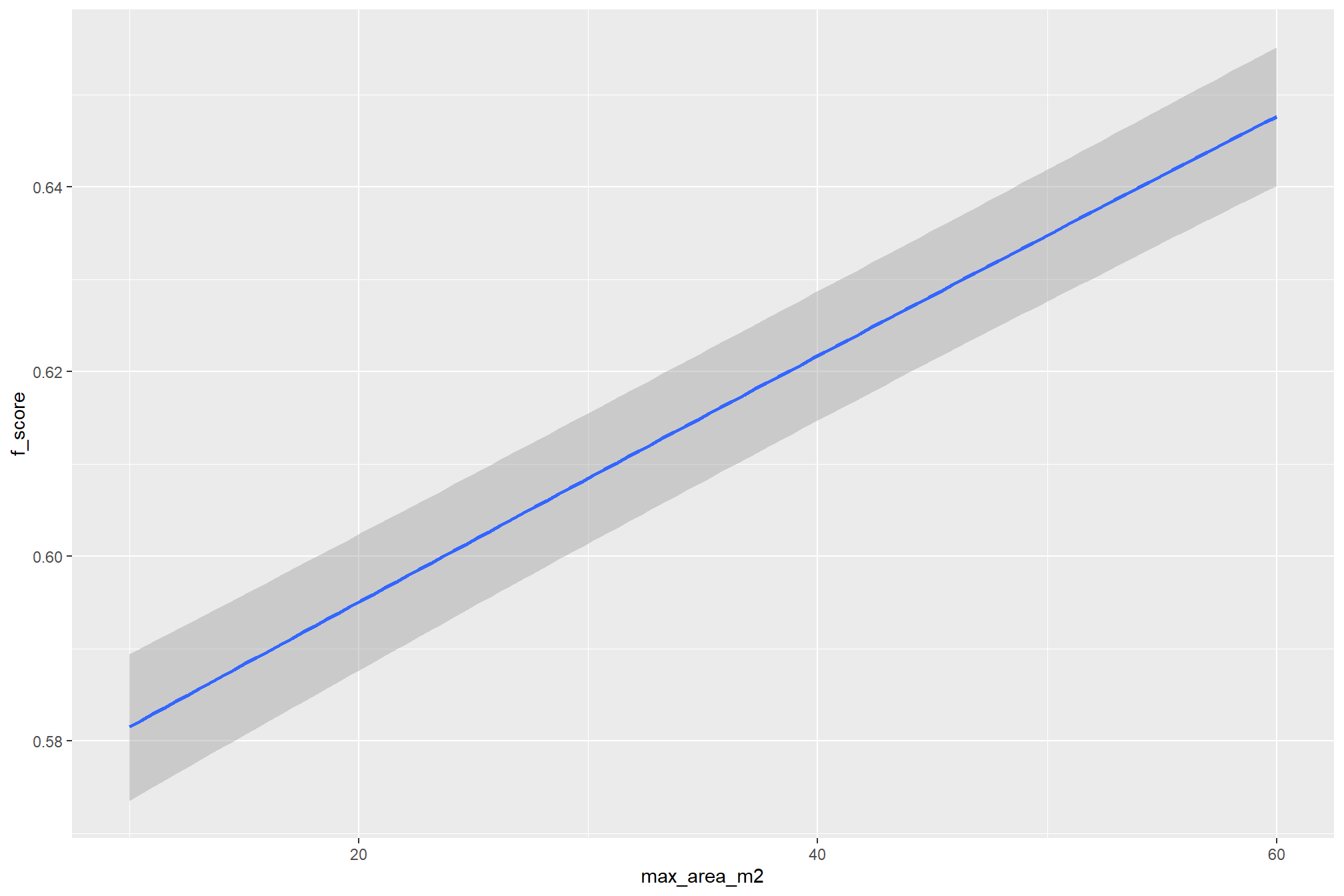
Our Bayesian Beta regression models the F-score with a Beta distribution because it is a proportion between 0 and 1, which ensures that the predictions and uncertainty estimates are always within the valid range. We’re treating the four structural parameters (e.g. max_ht_m and circle_fit_iou_pct) and the CHM resolution (chm_res_m) as metric (i.e., continuous) variables, as this is statistically sound for our data and allows for a continuous interpretation where the model coefficient will represent the change in F-score for a one-unit change in the parameter value. The spectral_weight parameter, however, will be treated as nominal to capture its discrete effects without assuming a linear relationship.
9.1.1 Model selection
we’re going to use a sub-sample of the data to perform model testing. our objective is to construct the model such that it faithfully represents the data.
we reviewed the main effect parameter trends against F-score here and used these to guide our model design. we’ll follow Kurz 2025 and compare our models with the LOO information criterion
Like other information criteria, the LOO values aren’t of interest in and of themselves. However, the values of one model’s LOO relative to that of another is of great interest. We generally prefer models with lower estimates.
# subsample data
set.seed(222)
ms_df_temp <- param_combos_spectral_ranked %>% dplyr::slice_sample(prop = 0.11)
# mcmc setup
iter_temp <- 2444
warmup_temp <- 1222
chains_temp <- 4
####################################################################
# base model with form selected based on main effect trends
####################################################################
fscore_mod1_temp <- brms::brm(
  formula = f_score ~
    0 + # no intercept to allow all values of spectral_weight to be shown instead of set as the baseline
    max_ht_m + max_area_m2 + convexity_pct +
    circle_fit_iou_pct + I(circle_fit_iou_pct^2) +
    chm_res_m + spectral_weight + chm_res_m:spectral_weight
  , data = ms_df_temp
  , family = Beta(link = "logit")
  # mcmc
  , iter = iter_temp, warmup = warmup_temp
  , chains = chains_temp
  # , control = list(adapt_delta = 0.999, max_treedepth = 13)
  , cores = lasR::half_cores()
  , file = paste0("../data/", "fscore_mod1_temp")
)
fscore_mod1_temp <- brms::add_criterion(fscore_mod1_temp, criterion = "loo")
####################################################################
# allows slope and curvature of circle_fit_iou_pct to vary by chm_res_m and vice-versa
####################################################################
fscore_mod2_temp <- brms::brm(
  formula = f_score ~
    0 + # no intercept to allow all values of spectral_weight to be shown instead of set as the baseline
    max_ht_m + max_area_m2 + convexity_pct +
    circle_fit_iou_pct + I(circle_fit_iou_pct^2) +
    circle_fit_iou_pct:chm_res_m + # changed from base model
    chm_res_m + spectral_weight + chm_res_m:spectral_weight
  , data = ms_df_temp
  , family = Beta(link = "logit")
  # mcmc
  , iter = iter_temp, warmup = warmup_temp
  , chains = chains_temp
  # , control = list(adapt_delta = 0.999, max_treedepth = 13)
  , cores = lasR::half_cores()
  , file = paste0("../data/", "fscore_mod2_temp")
)
fscore_mod2_temp <- brms::add_criterion(fscore_mod2_temp, criterion = "loo")
####################################################################
# allows slope and curvature of circle_fit_iou_pct to vary by convexity_pct and vice-versa
####################################################################
fscore_mod3_temp <- brms::brm(
  formula = f_score ~
    0 + # no intercept to allow all values of spectral_weight to be shown instead of set as the baseline
    max_ht_m + max_area_m2 + convexity_pct +
    circle_fit_iou_pct + I(circle_fit_iou_pct^2) +
    circle_fit_iou_pct:convexity_pct + # changed from base model
    chm_res_m + spectral_weight + chm_res_m:spectral_weight
  , data = ms_df_temp
  , family = Beta(link = "logit")
  # mcmc
  , iter = iter_temp, warmup = warmup_temp
  , chains = chains_temp
  # , control = list(adapt_delta = 0.999, max_treedepth = 13)
  , cores = lasR::half_cores()
  , file = paste0("../data/", "fscore_mod3_temp")
)
fscore_mod3_temp <- brms::add_criterion(fscore_mod3_temp, criterion = "loo")
####################################################################
# a three-way interaction of circle_fit_iou_pct, convexity_pct and chm_res_m
####################################################################
fscore_mod4_temp <- brms::brm(
  formula = f_score ~
    0 + # no intercept to allow all values of spectral_weight to be shown instead of set as the baseline
    max_ht_m + max_area_m2 + convexity_pct +
    circle_fit_iou_pct + I(circle_fit_iou_pct^2) +
    circle_fit_iou_pct:convexity_pct + # changed from base model
    circle_fit_iou_pct:chm_res_m + # changed from base model
    convexity_pct:chm_res_m + # changed from base model
    circle_fit_iou_pct:chm_res_m:convexity_pct + # changed from base model
    chm_res_m + spectral_weight + chm_res_m:spectral_weight
  , data = ms_df_temp
  , family = Beta(link = "logit")
  # mcmc
  , iter = iter_temp, warmup = warmup_temp
  , chains = chains_temp
  # , control = list(adapt_delta = 0.999, max_treedepth = 13)
  , cores = lasR::half_cores()
  , file = paste0("../data/", "fscore_mod4_temp")
)
fscore_mod4_temp <- brms::add_criterion(fscore_mod4_temp, criterion = "loo")
####################################################################
# a three-way interaction of circle_fit_iou_pct, convexity_pct and chm_res_m. quadratic convexity_pct
####################################################################
fscore_mod5_temp <- brms::brm(
  formula = f_score ~
    0 + # no intercept to allow all values of spectral_weight to be shown instead of set as the baseline
    max_ht_m + max_area_m2 +
    circle_fit_iou_pct + I(circle_fit_iou_pct^2) +
    convexity_pct + I(convexity_pct^2) +  # changed from base model
    circle_fit_iou_pct:convexity_pct + # changed from base model
    circle_fit_iou_pct:chm_res_m + # changed from base model
    convexity_pct:chm_res_m + # changed from base model
    circle_fit_iou_pct:chm_res_m:convexity_pct + # changed from base model
    chm_res_m + spectral_weight + chm_res_m:spectral_weight
  , data = ms_df_temp
  , family = Beta(link = "logit")
  # mcmc
  , iter = iter_temp, warmup = warmup_temp
  , chains = chains_temp
  # , control = list(adapt_delta = 0.999, max_treedepth = 13)
  , cores = lasR::half_cores()
  , file = paste0("../data/", "fscore_mod5_temp")
)
fscore_mod5_temp <- brms::add_criterion(fscore_mod4_temp, criterion = "loo")
compare our models with the LOO information criterion. with the brms::loo_compare() function, we can compute a formal difference score between models with the output rank ordering the models such that the best fitting model appears on top. all models also receive a difference score relative to the best model and a standard error of the difference score
brms::loo_compare(fscore_mod1_temp, fscore_mod2_temp, fscore_mod3_temp, fscore_mod4_temp, fscore_mod5_temp) %>%
  kableExtra::kbl(caption = "F-score model selection with LOO information criterion") %>%
kableExtra::kable_styling()| elpd_diff | se_diff | elpd_loo | se_elpd_loo | p_loo | se_p_loo | looic | se_looic | |
|---|---|---|---|---|---|---|---|---|
| fscore_mod4_temp | 0.0000 | 0.00000 | 4254.854 | 139.8614 | 26.42988 | 1.441628 | -8509.709 | 279.7227 |
| fscore_mod5_temp | 0.0000 | 0.00000 | 4254.854 | 139.8614 | 26.42988 | 1.441628 | -8509.709 | 279.7227 |
| fscore_mod3_temp | -216.3790 | 26.76322 | 4038.475 | 139.5926 | 27.71362 | 1.931427 | -8076.951 | 279.1851 |
| fscore_mod2_temp | -229.8413 | 28.35355 | 4025.013 | 138.5435 | 27.54291 | 1.893650 | -8050.026 | 277.0871 |
| fscore_mod1_temp | -234.9112 | 30.47721 | 4019.943 | 139.0671 | 27.27559 | 1.942107 | -8039.886 | 278.1342 |
we can also look at the AIC-type model weights
brms::model_weights(fscore_mod1_temp, fscore_mod2_temp, fscore_mod3_temp, fscore_mod4_temp, fscore_mod5_temp) %>%
  round(digits = 4)
we can also quickly look at the Bayeisan \(R^2\) returned from the brms::bayes_R2() function
dplyr::bind_rows(
  brms::bayes_R2(fscore_mod1_temp,summary=F) %>% dplyr::as_tibble() %>% dplyr::mutate(mod = "fscore_mod1_temp")
  , brms::bayes_R2(fscore_mod2_temp,summary=F) %>% dplyr::as_tibble() %>% dplyr::mutate(mod = "fscore_mod2_temp")
  , brms::bayes_R2(fscore_mod3_temp,summary=F) %>% dplyr::as_tibble() %>% dplyr::mutate(mod = "fscore_mod3_temp")
  , brms::bayes_R2(fscore_mod4_temp,summary=F) %>% dplyr::as_tibble() %>% dplyr::mutate(mod = "fscore_mod4_temp")
  , brms::bayes_R2(fscore_mod5_temp,summary=F) %>% dplyr::as_tibble() %>% dplyr::mutate(mod = "fscore_mod5_temp")
) %>%
  dplyr::mutate(mod = factor(mod)) %>%
  ggplot2::ggplot(mapping=ggplot2::aes(y=R2, x = mod)) +
  tidybayes::stat_eye(
    point_interval = median_hdi, .width = .95
    , slab_alpha = 0.95
  ) +
  # ggplot2::facet_grid(cols = dplyr::vars(spectral_weight)) +
  # ggplot2::scale_fill_manual(values = pal_chm_res_m) +
  ggplot2::labs(x = "", y = "Bayesian R-squared") +
  ggplot2::theme_light()
the more complex models were selected as the best. while our model evaluation indicated that the more parsimonious model with fewer parameters was comparable to the most complex model tested, we’ll the more complex model (fscore_mod5_temp) model for our based on the AIC-type model weights. because the selected model includes a quadratic term and multiple interactions parameter interpretation will be a challenge, so we will have to rely on plotting the modeled relationships rather than trying to interpret the coefficients.
9.1.2 Modeling
the four structural parameters (e.g. max_ht_m and circle_fit_iou_pct) and the CHM resolution (chm_res_m) as metric (i.e., continuous) variables. we include an interaction between chm_res_m and spectral_weight to directly compare the effect of CHM resolution with and without the use of spectral data.
we’ll generally follow Kurz (2023a; 2023b; 2025 for multiple linear regression model building using the brms Bayesian model framework based on McElreath (2015, Ch. 5,7) and Kruschke (2015, Ch. 18)
the fully factored Bayesian statistical model that details the likelihood, linear model, and priors used is:
\[\begin{align*} \text{F-score}_i \sim & \operatorname{Beta}(\mu_{i}, \phi) \\ \operatorname{logit}(\mu_i) = & (\beta_1 \cdot \text{max_ht_m}_i) + (\beta_2 \cdot \text{max_area_m2}_i) \\ & + (\beta_3 \cdot \text{circle_fit_iou_pct}_i) + (\beta_4 \cdot (\text{circle_fit_iou_pct}_i)^2) \\ & + (\beta_5 \cdot \text{convexity_pct}_i) + (\beta_6 \cdot (\text{convexity_pct}_i)^2) \\ & + (\beta_7 \cdot \text{chm_res_m}_i) \\ & + \sum_{j=0}^{5} \left( \beta_{8, j} \cdot \mathbf{I}(\text{spectral_weight}_i = j) \right) \\ & + (\beta_9 \cdot \text{circle_fit_iou_pct}_i \cdot \text{convexity_pct}_i) \\ & + (\beta_{10} \cdot \text{circle_fit_iou_pct}_i \cdot \text{chm_res_m}_i) \\ & + (\beta_{11} \cdot \text{convexity_pct}_i \cdot \text{chm_res_m}_i) \\ & + \sum_{j=0}^{5} \left( \beta_{12, j} \cdot \text{chm_res_m}_i \cdot \mathbf{I}(\text{spectral_weight}_i = j) \right) \\ & + (\beta_{13} \cdot \text{circle_fit_iou_pct}_i \cdot \text{chm_res_m}_i \cdot \text{convexity_pct}_i) \\ \beta_k \sim & \operatorname{Normal}(0, \sigma_k) \quad \text{for } k = 0, \dots, 13 \\ \sigma_k \sim & \operatorname{Student T}(3,0,2.5) \quad \text{for } k = 0, \dots, 13 \\ \phi \sim & \operatorname{Gamma}(0.01,0.01) \\ \end{align*}\]
where, \(i\) represents a single observation in the dataset which corresponds to a specific combination of the six parameters (max_ht_m, max_area_m2, convexity_pct, circle_fit_iou_pct, chm_res_m, and spectral_weight) and its resulting F-score. Where k is used to index the different beta coefficients, which correspond to the intercept and the effects of each of the independent variables and their interactions and j denotes the specific level of the nominal (i.e. categorical) predictor spectral_weight
let’s fit the model using the brms framework to fit Bayesian regression models using the Stan probabilistic programming language. if we want to set the prior for \(\beta_0\) given a non-centered predictors, then we need to use the 0 + Intercept syntax to fit the model (see Kurz 2025 for full discussion), but we’ll just fit the model with the brsm::brm() default settings which automatically mean centers the predictors and also set the intercept to 0 so that we get explicit coefficient estimates for each level of our spectral_weight nominal variable which determines the intercept in this model
The table below details the terms used in our Bayesian GLM model defined in the brms::brm() call:
| Term in Formula | Type of Effect | Description of Relationship Tested |
|---|---|---|
0 + |
Zero Intercept | Specifies that the model is fit without a global intercept (baseline is determined by the combination of all factor levels). |
max_ht_m |
Main Effect (Linear) | Tests the direct, isolated linear influence of the maximum pile height threshold on the F-score. |
max_area_m2 |
Main Effect (Linear) | Tests the direct, isolated linear influence of the maximum pile area threshold on the F-score. |
chm_res_m |
Main Effect (Linear) | Tests the direct, isolated linear influence of the input Canopy Height Model (CHM) resolution on the F-score. |
spectral_weight |
Main Effect (Factor) | The model estimates a separate coefficient for each of the six spectral weight levels (0 through 5). This coefficient represents the estimated mean F-score for that specific spectral weight level when all continuous variables are zero. |
circle_fit_iou_pct |
Main Effect (Linear) | Tests the direct linear influence of the pile’s circular conformity threshold on the F-score. |
convexity_pct |
Main Effect (Linear) | Tests the direct linear influence of the pile’s boundary smoothness (convexity) threshold on the F-score. |
I(circle_fit_iou_pct^2) |
Nonlinear (Quadratic) | Models a curved relationship where the F-score may peak or bottom out at an intermediate threshold for pile circularity. |
I(convexity_pct^2) |
Nonlinear (Quadratic) | Models a curved relationship where the F-score may peak or bottom out at an intermediate threshold for pile boundary smoothness. |
circle_fit_iou_pct:convexity_pct |
Two-Way Interaction | Captures how the optimal balance between pile circular conformity and boundary smoothness changes for the F-score. |
chm_res_m:spectral_weight |
Two-Way Interaction (Factor) | Captures how the effect of CHM resolution on the F-score changes across each of the six spectral weighting levels. |
circle_fit_iou_pct:chm_res_m |
Two-Way Interaction | Captures how the importance of the pile’s circular conformity threshold changes as the input data resolution changes. |
convexity_pct:chm_res_m |
Two-Way Interaction | Captures how the sensitivity to the pile boundary smoothness threshold changes with the input data resolution. |
circle_fit_iou_pct:chm_res_m:convexity_pct |
Three-Way Interaction | The most complex term, showing how the combined effects of the circularity and convexity thresholds change simultaneously across different input CHM resolutions. |
brms_f_score_mod <- brms::brm(
  formula = f_score ~
    0 + # no intercept to allow all values of spectral_weight to be shown instead of set as the baseline
    max_ht_m + max_area_m2 +
    circle_fit_iou_pct + I(circle_fit_iou_pct^2) +
    convexity_pct + I(convexity_pct^2) +  # changed from base model
    circle_fit_iou_pct:convexity_pct + # changed from base model
    circle_fit_iou_pct:chm_res_m + # changed from base model
    convexity_pct:chm_res_m + # changed from base model
    circle_fit_iou_pct:chm_res_m:convexity_pct + # changed from base model
    chm_res_m + spectral_weight + chm_res_m:spectral_weight
  , data = param_combos_spectral_ranked # %>% dplyr::slice_sample(prop = 0.33)
  , family = Beta(link = "logit")
  # , prior = c(
  #   brms::prior(student_t(3, 0, 5), class = "b")
  #   , brms::prior(gamma(0.01, 0.01), class = "phi")
  # )
  # mcmc
  , iter = 14000, warmup = 7000
  , chains = 4
  # , control = list(adapt_delta = 0.999, max_treedepth = 13)
  , cores = lasR::half_cores()
  , file = paste0("../data/", "brms_f_score_mod")
)
# brms::make_stancode(brms_f_score_mod)
# brms::prior_summary(brms_f_score_mod)
# print(brms_f_score_mod)
# brms::neff_ratio(brms_f_score_mod)
# brms::rhat(brms_f_score_mod)
# brms::nuts_params(brms_f_score_mod)
The brms::brm model summary
brms_f_score_mod %>%
  brms::posterior_summary() %>%
  as.data.frame() %>%
  tibble::rownames_to_column(var = "parameter") %>%
  dplyr::rename_with(tolower) %>%
  dplyr::filter(
    stringr::str_starts(parameter, "b_")
    | parameter == "phi"
  ) %>%
  # dplyr::mutate(
  #   dplyr::across(
  #     dplyr::where(is.numeric)
  #     , ~ dplyr::case_when(
  #       stringr::str_ends(parameter,"_pct") ~ .x*0.01 # convert to percentage point change
  #       , T ~ .x
  #     )
  #   )
  # ) %>%
  kableExtra::kbl(digits = 3, caption = "Bayesian model for F-score") %>%
kableExtra::kable_styling()| parameter | estimate | est.error | q2.5 | q97.5 |
|---|---|---|---|---|
| b_max_ht_m | -0.033 | 0.004 | -0.042 | -0.025 |
| b_max_area_m2 | 0.006 | 0.000 | 0.005 | 0.006 |
| b_circle_fit_iou_pct | 5.893 | 0.100 | 5.696 | 6.091 |
| b_Icircle_fit_iou_pctE2 | -9.792 | 0.066 | -9.923 | -9.662 |
| b_convexity_pct | 0.297 | 0.103 | 0.094 | 0.498 |
| b_Iconvexity_pctE2 | -5.165 | 0.065 | -5.291 | -5.037 |
| b_chm_res_m | -6.767 | 0.159 | -7.081 | -6.456 |
| b_spectral_weight0 | 0.897 | 0.057 | 0.786 | 1.010 |
| b_spectral_weight1 | 0.896 | 0.057 | 0.785 | 1.008 |
| b_spectral_weight2 | 0.896 | 0.057 | 0.786 | 1.009 |
| b_spectral_weight3 | 0.925 | 0.057 | 0.814 | 1.038 |
| b_spectral_weight4 | 1.209 | 0.056 | 1.099 | 1.320 |
| b_spectral_weight5 | 1.083 | 0.056 | 0.973 | 1.195 |
| b_circle_fit_iou_pct:convexity_pct | 2.815 | 0.127 | 2.569 | 3.065 |
| b_circle_fit_iou_pct:chm_res_m | 2.690 | 0.230 | 2.240 | 3.141 |
| b_convexity_pct:chm_res_m | 10.563 | 0.232 | 10.105 | 11.020 |
| b_chm_res_m:spectral_weight1 | 0.001 | 0.120 | -0.234 | 0.237 |
| b_chm_res_m:spectral_weight2 | 0.001 | 0.121 | -0.236 | 0.238 |
| b_chm_res_m:spectral_weight3 | 0.000 | 0.120 | -0.235 | 0.236 |
| b_chm_res_m:spectral_weight4 | -0.263 | 0.117 | -0.491 | -0.033 |
| b_chm_res_m:spectral_weight5 | 0.628 | 0.115 | 0.403 | 0.853 |
| b_circle_fit_iou_pct:convexity_pct:chm_res_m | -6.991 | 0.407 | -7.789 | -6.188 |
| phi | 4.170 | 0.031 | 4.110 | 4.230 |
note the quadratic coefficients ending in E2, Kruschke (2015) provides some insight on how to interpret:
A quadratic has the form \(y = \beta_{0} + \beta_{1}x + \beta_{2}x^{2}\). When \(\beta_{2}\) is zero, the form reduces to a line. Therefore, this extended model can produce any fit that the linear model can. When \(\beta_{2}\) is positive, a plot of the curve is a parabola that opens upward. When \(\beta_{2}\) is negative, the curve is a parabola that opens downward. We have no reason to think that the curvature in the family-income data is exactly a parabola, but the quadratic trend might describe the data much better than a line alone. (p. 496)
9.1.3 Posterior Predictive Checks
Markov chain Monte Carlo (MCMC) simulations were conducted using the brms package (Bürkner 2017) to estimate posterior predictive distributions of the parameters of interest. We ran 4 chains of 14,000 iterations with the first 7,000 discarded as burn-in. Trace-plots were utilized to visually assess model convergence.
check the trace plots for problems with convergence of the Markov chains

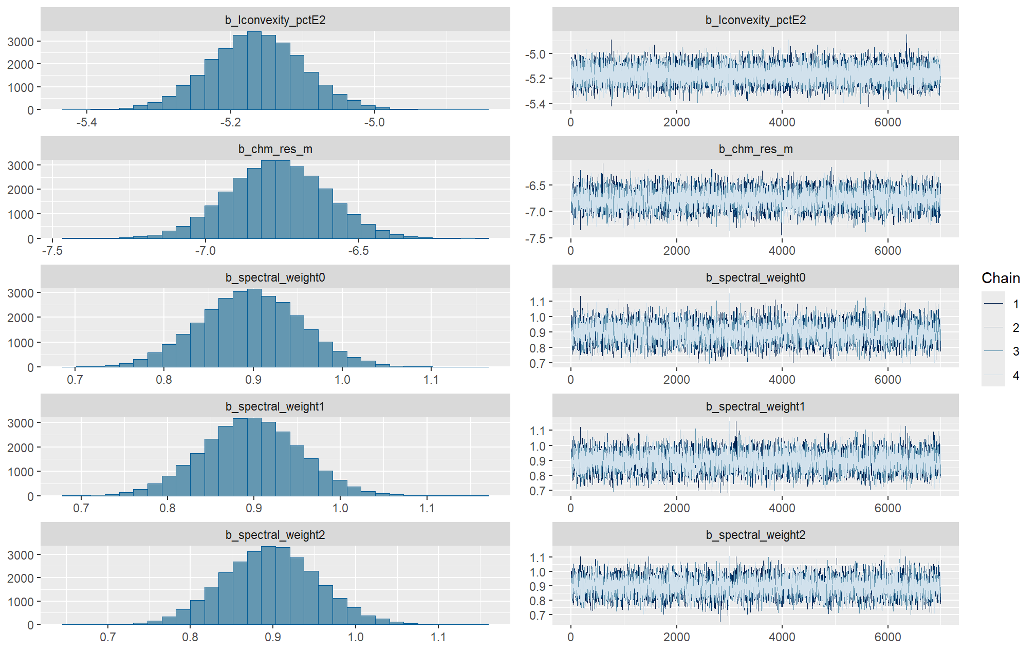

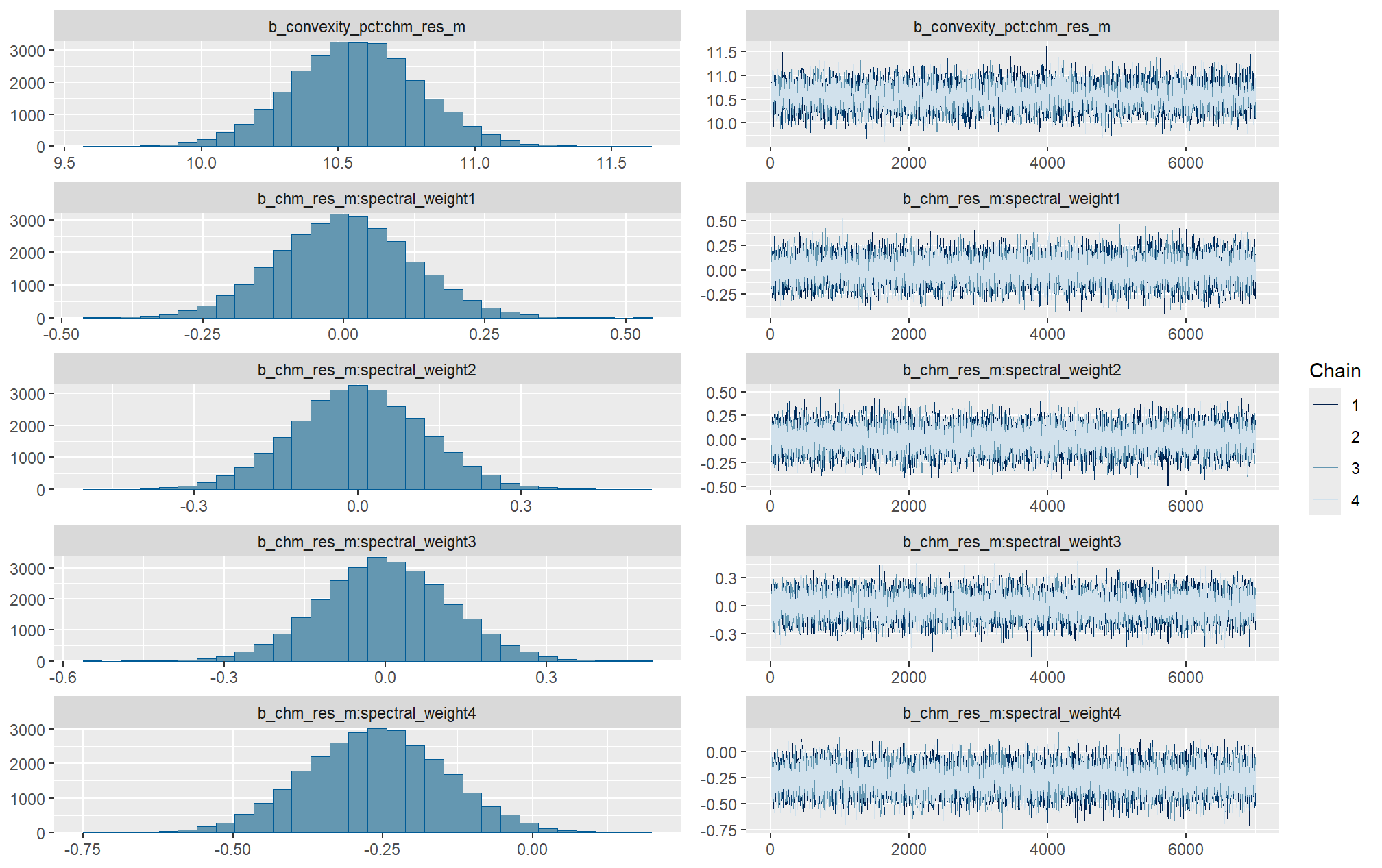
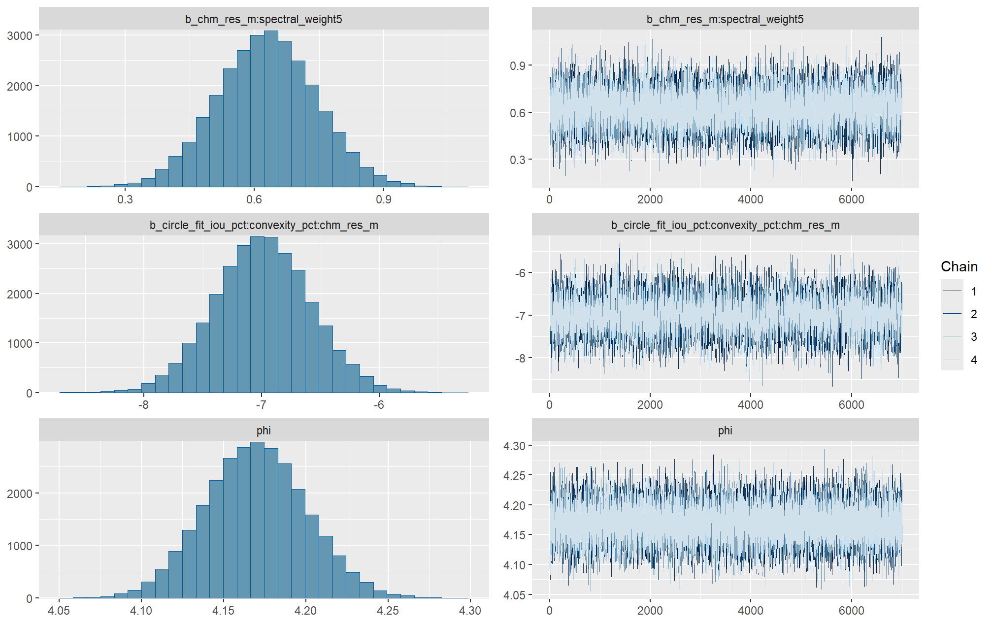
Sufficient convergence was checked with \(\hat{R}\) values near 1 (Brooks & Gelman, 1998).
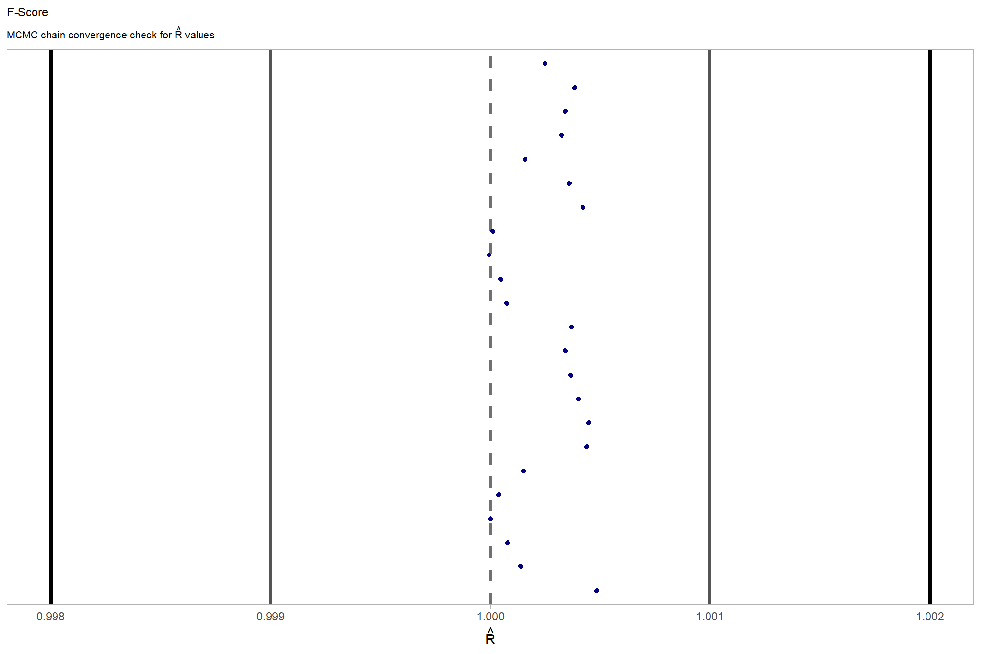
in the plot below, \(\hat{R}\) values are colored using different shades (lighter is better). The chosen thresholds are somewhat arbitrary, but can be useful guidelines in practice (Gabry and Mahr 2025):
- light: below 1.05 (good)
- mid: between 1.05 and 1.1 (ok)
- dark: above 1.1 (too high)
check our \(\hat{R}\) values
brms::mcmc_plot(brms_f_score_mod, type = "rhat_hist") +
  ggplot2::scale_x_continuous(breaks = scales::breaks_extended(n = 6)) +
  ggplot2::theme_light() +
  ggplot2::theme(
    legend.position = "top", legend.direction = "horizontal"
  )
and another check of our \(\hat{R}\) values
# and another check of our $\hat{R}$ values
brms_f_score_mod %>%
  brms::rhat() %>%
  as.data.frame() %>%
  tibble::rownames_to_column(var = "parameter") %>%
  dplyr::rename_with(tolower) %>%
  dplyr::rename(rhat = 2) %>%
  dplyr::filter(
    stringr::str_starts(parameter, "b_")
    | stringr::str_starts(parameter, "r_")
    | stringr::str_starts(parameter, "sd_")
    | parameter == "phi"
  ) %>%
  dplyr::mutate(
    chk = (rhat <= 1*0.998 | rhat >= 1*1.002)
  ) %>%
  ggplot(aes(x = rhat, y = parameter, color = chk, fill = chk)) +
  geom_vline(xintercept = 1, linetype = "dashed", color = "gray44", lwd = 1.2) +
  geom_vline(xintercept = 1*0.998, lwd = 1.5) +
  geom_vline(xintercept = 1*1.002, lwd = 1.5) +
  geom_vline(xintercept = 1*0.999, lwd = 1.2, color = "gray33") +
  geom_vline(xintercept = 1*1.001, lwd = 1.2, color = "gray33") +
  geom_point() +
  scale_fill_manual(values = c("navy", "firebrick")) +
  scale_color_manual(values = c("navy", "firebrick")) +
  scale_y_discrete(NULL, breaks = NULL) +
  labs(
    x = latex2exp::TeX("$\\hat{R}$")
    , subtitle = latex2exp::TeX("MCMC chain convergence check for $\\hat{R}$ values")
    , title = "F-Score"
  ) +
  theme_light() +
  theme(
    legend.position = "none"
    , axis.text.y = element_text(size = 4)
    , panel.grid.major.x = element_blank()
    , panel.grid.minor.x = element_blank()
    , plot.subtitle = element_text(size = 8)
    , plot.title = element_text(size = 9)
  )
The effective length of an MCMC chain is indicated by the effective sample size (ESS), which refers to the sample size of the MCMC chain not to the sample size of the data where acceptable values allow “for reasonably accurate and stable estimates of the limits of the 95% HDI…If accuracy of the HDI limits is not crucial for your application, then a smaller ESS may be sufficient” (Kruschke 2015, p. 184)
Ratios of effective sample size (ESS) to total sample size with values are colored using different shades (lighter is better). A ratio close to “1” (no autocorrelation) is ideal, while a low ratio suggests the need for more samples or model re-parameterization. Efficiently mixing MCMC chains are important because they guarantee the resulting posterior samples accurately represent the true distribution of model parameters, which is necessary for reliable and precise estimation of parameter values and their associated uncertainties (credible intervals). The chosen thresholds are somewhat arbitrary, but can be useful guidelines in practice (Gabry and Mahr 2025):
- light: between 0.5 and 1 (high)
- mid: between 0.1 and 0.5 (good)
- dark: below 0.1 (low)
# and another effective sample size check
brms::mcmc_plot(brms_f_score_mod, type = "neff_hist") +
# brms::mcmc_plot(brms_f_score_mod, type = "neff") +
  ggplot2::scale_x_continuous(limits = c(0,NA), breaks = scales::breaks_extended(n = 9)) +
  # ggplot2::scale_color_discrete(drop = F) +
  # ggplot2::scale_fill_discrete(drop = F) +
  ggplot2::theme_light() +
  ggplot2::theme(
    legend.position = "top", legend.direction = "horizontal"
  )
our observed range of ESS to Total Sample Size ratios (~0.2 to ~0.8) are generally considered good to excellent, indicating the MCMC chains are performing well and mixing efficiently
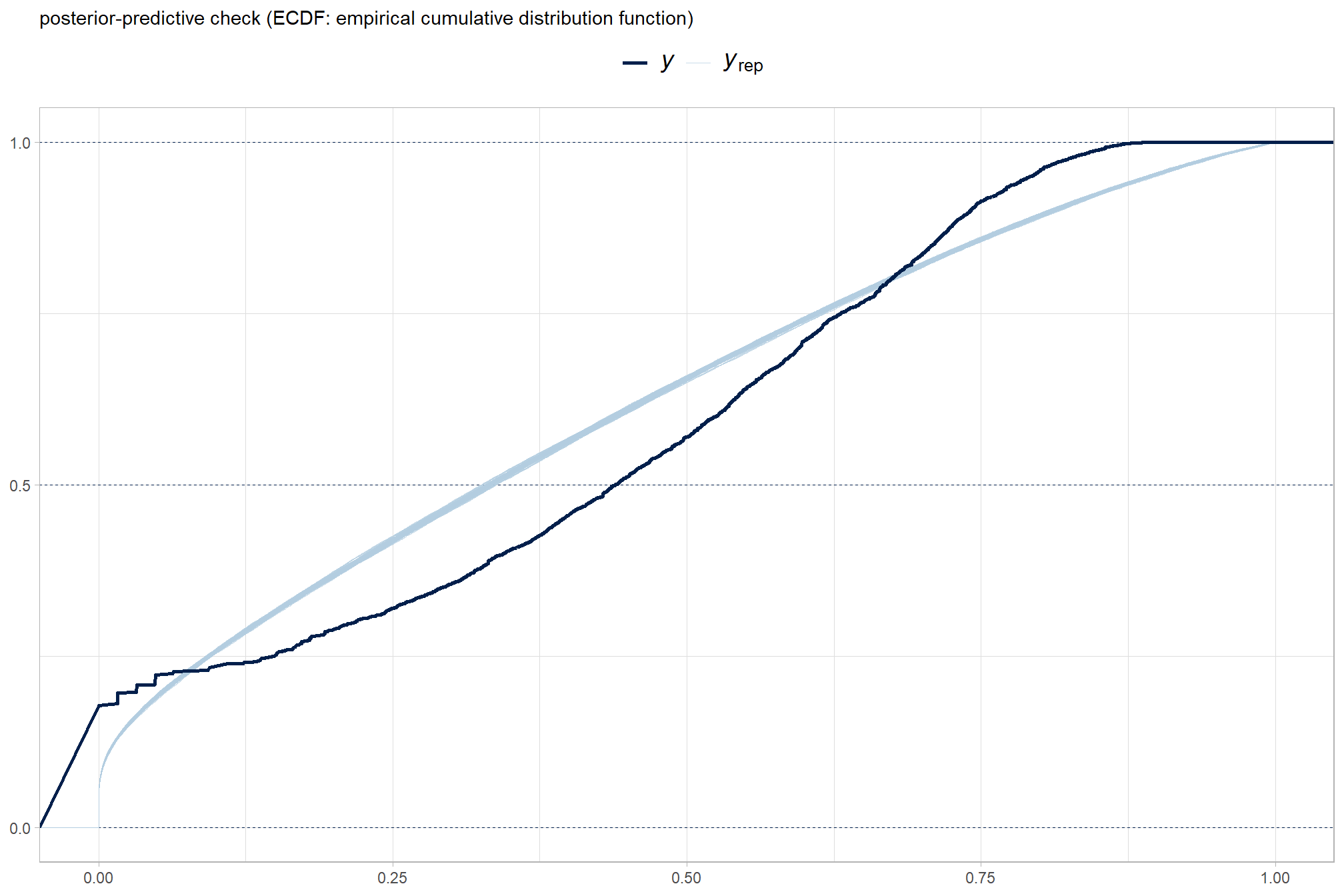
Posterior predictive checks were used to evaluate model goodness-of-fit by comparing data simulated from the model with the observed data used to estimate the model parameters (Hobbs & Hooten, 2015). Calculating the proportion of MCMC iterations in which the test statistic (i.e., mean and sum of squares) from the simulated data and observed data are more extreme than one another provides the Bayesian p-value. Lack of fit is indicated by a value close to 0 or 1 while a value of 0.5 indicates perfect fit (Hobbs & Hooten, 2015).
To learn more about this approach to posterior predictive checks, check out Gabry’s (2025) vignette, Graphical posterior predictive checks using the bayesplot package.
posterior-predictive check to make sure the model does an okay job simulating data that resemble the sample data. our objective is to construct the model such that it faithfully represents the data.
# posterior predictive check
brms::pp_check(
    brms_f_score_mod
    , type = "dens_overlay"
    , ndraws = 100
  ) +
  ggplot2::labs(subtitle = "posterior-predictive check (overlaid densities)") +
  ggplot2::theme_light() +
  ggplot2::scale_y_continuous(NULL, breaks = NULL) +
  ggplot2::theme(
    legend.position = "top", legend.direction = "horizontal"
    , legend.text = ggplot2::element_text(size = 14)
    , plot.subtitle = ggplot2::element_text(size = 8)
    , plot.title = ggplot2::element_text(size = 9)
  )
another way
brms::pp_check(brms_f_score_mod, type = "ecdf_overlay", ndraws = 100) +
  ggplot2::labs(subtitle = "posterior-predictive check (ECDF: empirical cumulative distribution function)") +
  ggplot2::theme_light() +
  ggplot2::theme(
    legend.position = "top", legend.direction = "horizontal"
    , legend.text = ggplot2::element_text(size = 14)
  )
9.1.4 Conditional Effects
first, lets look at densities of the posterior samples per parameter
brms::mcmc_plot(brms_f_score_mod, type = "dens") +
  # ggplot2::theme_light() +
  ggplot2::theme(
    strip.text = ggplot2::element_text(size = 7.5, face = "bold", color = "black")
  )
and we can look at the default coefficient plot that is commonly used in reporting coefficient “significance” in frequentist analysis
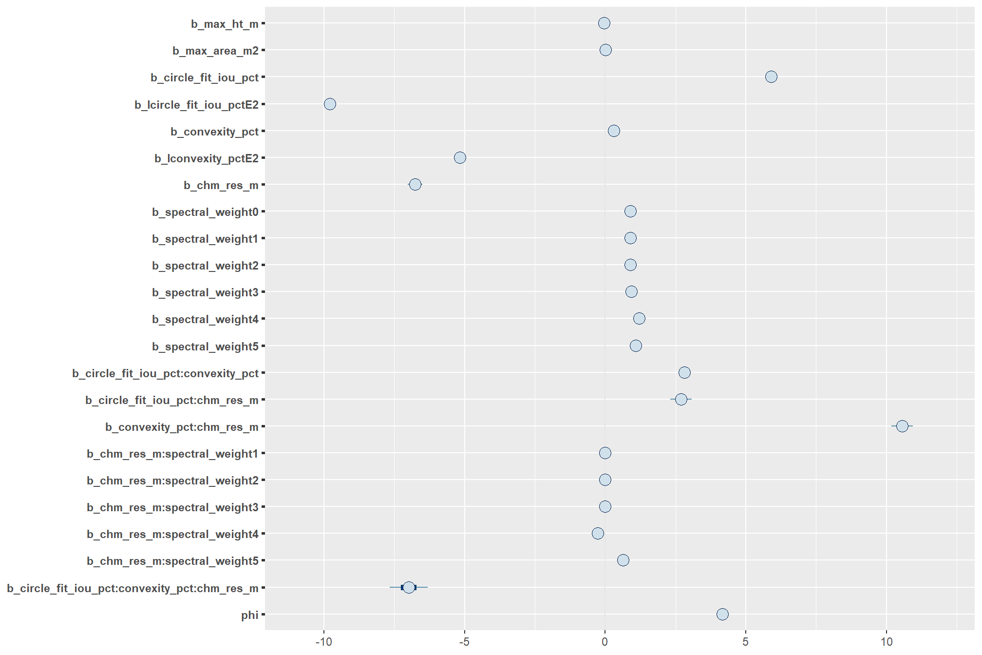
Regarding interactions and polynomial models like this, McElreath (2015) notes:
parameters are the linear and square components of the curve, respectively. But that doesn’t make them transparent. You have to plot these model fits to understand what they are saying. (p. 112-113)
all of the interactions and the quadradic trend of this model combine to make these coefficients by themselves uninterpretable as the coefficients are only meaningful in the context of the other terms in the interaction or by adding the quadratic component
we can do this by checking for the main effects of the individual variables on F-score (averages across all other effects)

### ggplot version
# brms::conditional_effects(brms_f_score_mod) %>%
#   purrr::pluck("max_ht_m") %>%
#   ggplot(aes(x = max_ht_m)) +
#   geom_ribbon(aes(ymin = lower__, ymax = upper__), fill = "blue", alpha = 0.2) +
#   geom_line(aes(y = estimate__), color = "blue") +
#   labs(
#     x = "max_ht_m",
#     y = "F-score",
#     title = "Conditional Effects"
#   )
9.1.5 Posterior Predictive Expectation
we will test our hypotheses using the posterior distributions of the expected values (i.e., the posterior predictions of the mean) obtained via tidybayes::add_epred_draws(). our analysis will include two stages using parameter levels of the four structural parameters: max_ht_m, max_area_m2, convexity_pct, circle_fit_iou_pct. in practice, these values should be informed by the treatment and slash pile construction prescription implemented on the ground.
In the first stage, we will fix the max_ht_m and max_area_m2 parameters at levels expected based on the treatment and slash pile construction prescription implemented on the ground. We will then explore the influence of the two geometric shape filtering parameters (circle_fit_iou_pct and convexity_pct) over different levels of the spectral_weight parameter and CHM resolution data.
In the second stage, we will fix all four structural parameters (max_ht_m, max_area_m2, convexity_pct, circle_fit_iou_pct) to explore the influence of the input data, which includes the presence or absence of spectral data and its weighting (i.e. spectral_weight) as well as the CHM resolution (chm_res_m). As in the first stage, the max_ht_m, max_area_m2 parameters will be fixed at expected levels based on the slash pile construction prescription while the convexity_pct, circle_fit_iou_pct will be fixed at the optimal levels determined based on the Bayesian posterior predictive distribution of detection accuracy
# let's fix the structural parameters based on expectations from the prescription
structural_params_settings <-
  dplyr::tibble(
    max_ht_m = 2.3
    , max_area_m2 = 46
  )
  # dplyr::bind_rows(
  #   # structural only
  #   param_combos_ranked %>% dplyr::filter(is_top_overall) %>% dplyr::select(max_ht_m,max_area_m2,convexity_pct,circle_fit_iou_pct)
  #   # fusion
  #   , param_combos_spectral_ranked %>%
  #     dplyr::ungroup() %>%
  #     dplyr::filter(is_top_overall & spectral_weight!=0) %>%
  #     dplyr::arrange(ovrall_balanced_rank) %>% # same number of records as structural only
  #     dplyr::filter(dplyr::row_number()<=sum(param_combos_ranked$is_top_overall)) %>%
  #     dplyr::select(max_ht_m,max_area_m2,convexity_pct,circle_fit_iou_pct)
  # ) %>%
  #   tidyr::pivot_longer(
  #     cols = dplyr::everything()
  #     , names_to = "metric"
  #     , values_to = "value"
  #   ) %>%
  #   dplyr::count(metric, value) %>%
  #   dplyr::group_by(metric) %>%
  #   dplyr::arrange(metric,desc(n),value) %>%
  #   dplyr::slice(1) %>%
  #   dplyr::select(-n) %>%
  #   tidyr::pivot_wider(names_from = metric, values_from = value) %>%
  #   dplyr::mutate(is_top_overall = T) %>%
  # # we just need `max_ht_m`, `max_area_m2`
  # dplyr::select(max_ht_m, max_area_m2)

# huh?
structural_params_settings %>% dplyr::glimpse()
## Rows: 1
## Columns: 2
## $ max_ht_m <dbl> 2.3
## $ max_area_m2 <dbl> 46now we’ll get the posterior predictive draws but over a range of circle_fit_iou_pct and convexity_pct including the best setting
seq_temp <- seq(from = 0.05, to = 1.0, by = 0.1)
seq2_temp <- seq_temp[seq(1, length(seq_temp), by = 2)] # get every other element
# draws
draws_temp <-
  # get the draws for levels of
  # spectral_weight circle_fit_iou_pct convexity_pct
  tidyr::crossing(
    param_combos_spectral_ranked %>% dplyr::distinct(spectral_weight)
    , circle_fit_iou_pct = seq_temp
    , convexity_pct = seq_temp
    , chm_res_m = seq(from = 0.1, to = 1.0, by = 0.1)
    , max_ht_m = structural_params_settings$max_ht_m
    , max_area_m2 = structural_params_settings$max_area_m2
  ) %>%
  # dplyr::glimpse()
  tidybayes::add_epred_draws(brms_f_score_mod, ndraws = 1111) %>%
  dplyr::rename(value = .epred) %>%
  dplyr::mutate(
    is_seq = (convexity_pct %in% seq_temp) & (circle_fit_iou_pct %in% seq_temp)
  )
# # huh?
draws_temp %>% dplyr::glimpse()
## Rows: 6,666,000
## Columns: 12
## Groups: spectral_weight, circle_fit_iou_pct, convexity_pct, chm_res_m, max_ht_m, max_area_m2, .row [6,000]
## $ spectral_weight <fct> 0, 0, 0, 0, 0, 0, 0, 0, 0, 0, 0, 0, 0, 0, 0, 0, 0, …
## $ circle_fit_iou_pct <dbl> 0.05, 0.05, 0.05, 0.05, 0.05, 0.05, 0.05, 0.05, 0.0…
## $ convexity_pct <dbl> 0.05, 0.05, 0.05, 0.05, 0.05, 0.05, 0.05, 0.05, 0.0…
## $ chm_res_m <dbl> 0.1, 0.1, 0.1, 0.1, 0.1, 0.1, 0.1, 0.1, 0.1, 0.1, 0…
## $ max_ht_m <dbl> 2.3, 2.3, 2.3, 2.3, 2.3, 2.3, 2.3, 2.3, 2.3, 2.3, 2…
## $ max_area_m2 <dbl> 46, 46, 46, 46, 46, 46, 46, 46, 46, 46, 46, 46, 46,…
## $ .row <int> 1, 1, 1, 1, 1, 1, 1, 1, 1, 1, 1, 1, 1, 1, 1, 1, 1, …
## $ .chain <int> NA, NA, NA, NA, NA, NA, NA, NA, NA, NA, NA, NA, NA,…
## $ .iteration <int> NA, NA, NA, NA, NA, NA, NA, NA, NA, NA, NA, NA, NA,…
## $ .draw <int> 1, 2, 3, 4, 5, 6, 7, 8, 9, 10, 11, 12, 13, 14, 15, …
## $ value <dbl> 0.6778712, 0.6924090, 0.6793626, 0.6784690, 0.69338…
## $ is_seq <lgl> TRUE, TRUE, TRUE, TRUE, TRUE, TRUE, TRUE, TRUE, TRU…9.1.5.1 Geometric shape regularity
let’s look at the influence of the parameters that control the geometric shape regularity filtering: circle_fit_iou_pct and convexity_pct. to do this, we will fix the max_ht_m and max_area_m2 parameters at levels expected based on the treatment and slash pile construction prescription implemented on the ground.
In the first stage, we will fix the max_ht_m and max_area_m2 parameters at levels expected based on the treatment and slash pile construction prescription implemented on the ground. We will then explore the influence of the two geometric shape filtering parameters (circle_fit_iou_pct and convexity_pct) over different levels of the spectral_weight parameter and CHM resolution data.
In the second stage, we will fix all four structural parameters (max_ht_m, max_area_m2, convexity_pct, circle_fit_iou_pct) to explore the influence of the input data, which includes the presence or absence of spectral data and its weighting (i.e. spectral_weight) as well as the CHM resolution (chm_res_m). As in the first stage, the max_ht_m, max_area_m2 parameters will be fixed at expected levels based on the slash pile construction prescription while the convexity_pct, circle_fit_iou_pct will be fixed at the optimal levels determined based on the Bayesian posterior predictive distribution of detection accuracy
9.1.5.1.1 circle_fit_iou_pct
we need to look at the influence of circle_fit_iou_pct in the context of the other terms in the interaction
draws_temp %>%
  dplyr::ungroup() %>%
  dplyr::filter(
    is_seq
    , chm_res_m %in% seq(0.1,0.5,by=0.1)
    , convexity_pct %in% seq2_temp
  ) %>%
  dplyr::mutate(convexity_pct = factor(convexity_pct, ordered = T)) %>%
  ggplot2::ggplot(mapping = ggplot2::aes(x = circle_fit_iou_pct, y = value, color = convexity_pct)) +
  tidybayes::stat_lineribbon(
    point_interval = "median_hdi", .width = c(0.95)
    , lwd = 1.1, fill = NA
  ) +
  ggplot2::facet_grid(cols = dplyr::vars(spectral_weight), rows = dplyr::vars(chm_res_m), labeller = "label_both") +
  ggplot2::scale_fill_brewer(palette = "Greys") +
  ggplot2::scale_color_viridis_d(option = "mako", begin = 0.6, end = 0.1) +
  ggplot2::scale_y_continuous(labels = scales::percent) +
  ggplot2::labs(
    title = "conditional effect of `circle_fit_iou_pct` on F-score"
    # , subtitle = "Faceted by spectral_weight and chm_res_m"
    , x = "`circle_fit_iou_pct`"
    , y = "F-score"
    , color = "`convexity_pct`"
  ) +
  ggplot2::theme_light() +
  ggplot2::theme(
    legend.position = "top"
    , strip.text.x = ggplot2::element_text(size = 10, color = "black", face = "bold")
    , strip.text.y = ggplot2::element_text(size = 10, color = "black", face = "bold")
  ) +
  ggplot2::guides(
    color = ggplot2::guide_legend(override.aes = list(shape = 15, lwd = 8, fill = NA))
    , fill = "none"
  )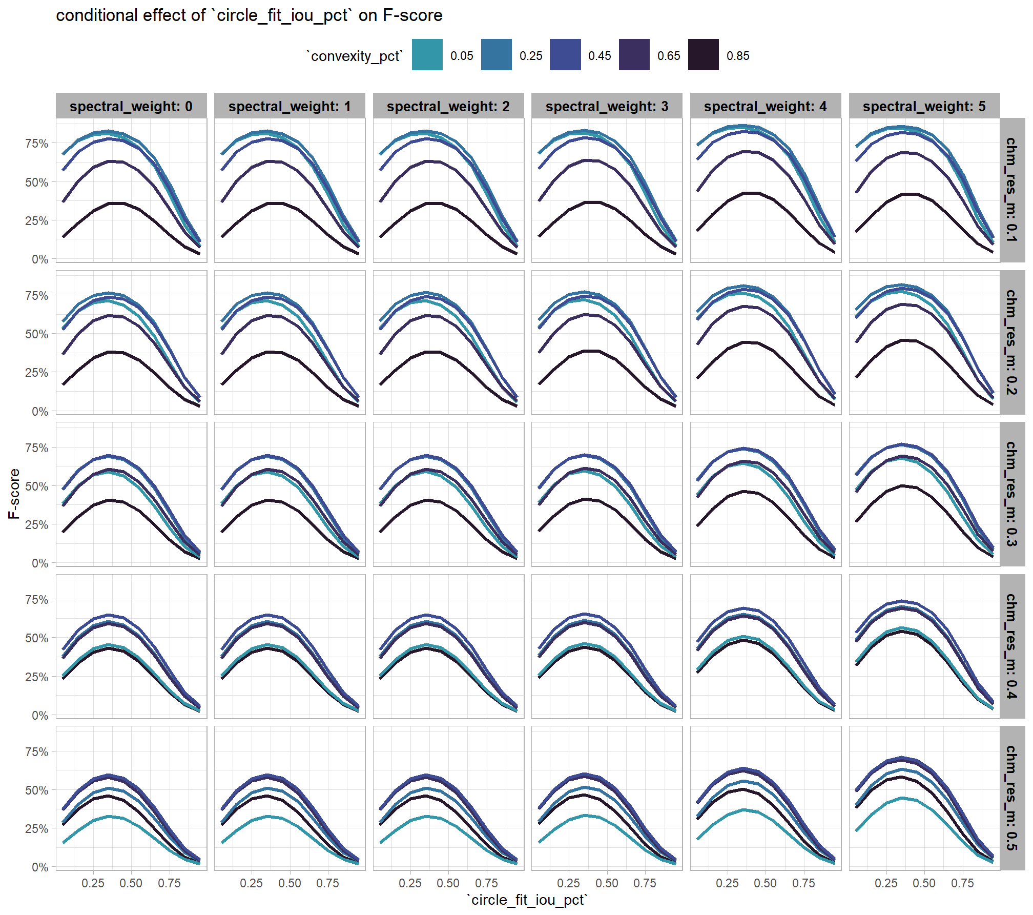
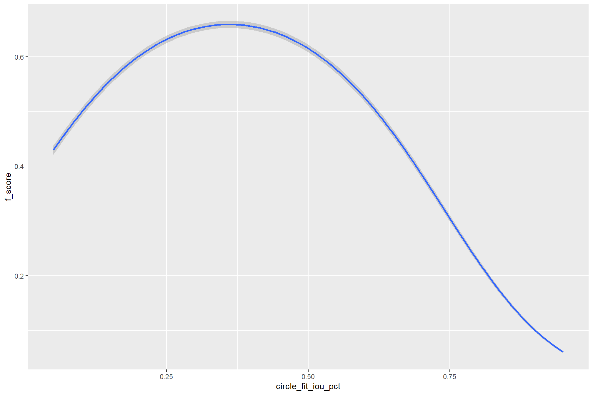
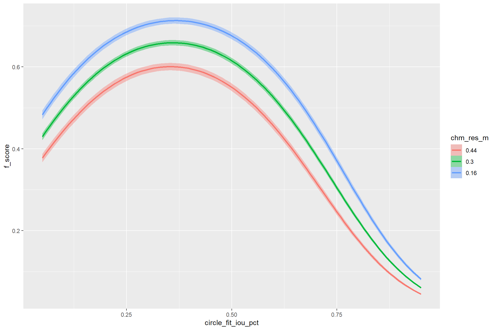
the non-linear relationship between the circle_fit_iou_pct parameter and the F-score is prominent, confirmed by the model’s quadratic coefficient. this trend is consistent across all levels of spectral_weight and CHM resolution. this figure also demonstrates how, within the optimal range of circle_fit_iou_pct, the intermediate values of the convexity_pct parameter seem to result in the best detection accuracy across CHM resolution levels. Across all CHM resolutions and spectral weighting levels, setting circle_fit_iou_pct too high (e.g > 0.7) results in steep declines in detection accuracy.
9.1.5.1.2 convexity_pct
we need to look at the influence of convexity_pct in the context of the other terms in the interaction
draws_temp %>%
  dplyr::ungroup() %>%
  dplyr::filter(
    is_seq
    , chm_res_m %in% seq(0.1,0.5,by=0.1)
    , circle_fit_iou_pct %in% seq2_temp
  ) %>%
  dplyr::mutate(circle_fit_iou_pct = factor(circle_fit_iou_pct, ordered = T)) %>%
  ggplot2::ggplot(mapping = ggplot2::aes(x = convexity_pct, y = value, color = circle_fit_iou_pct)) +
  tidybayes::stat_lineribbon(
    point_interval = "median_hdi", .width = c(0.5,0.95)
    , lwd = 1.1
    , fill = NA
  ) +
  ggplot2::facet_grid(cols = dplyr::vars(spectral_weight), rows = dplyr::vars(chm_res_m), labeller = "label_both") +
  ggplot2::scale_fill_brewer(palette = "Greys") +
  ggplot2::scale_color_viridis_d(option = "magma", begin = 0.5, end = 0.1) +
  ggplot2::scale_y_continuous(labels = scales::percent) +
  ggplot2::labs(
    title = "conditional effect of `convexity_pct` on F-score"
    # , subtitle = "Faceted by spectral_weight and chm_res_m"
    , x = "`convexity_pct`"
    , y = "F-score"
    , color = "`circle_fit_iou_pct`"
  ) +
  ggplot2::theme_light() +
  ggplot2::theme(
    legend.position = "top"
    , strip.text.x = ggplot2::element_text(size = 10, color = "black", face = "bold")
    , strip.text.y = ggplot2::element_text(size = 10, color = "black", face = "bold")
  ) +
  ggplot2::guides(
    color = ggplot2::guide_legend(override.aes = list(shape = 15, lwd = 8, fill = NA))
    , fill = "none"
  )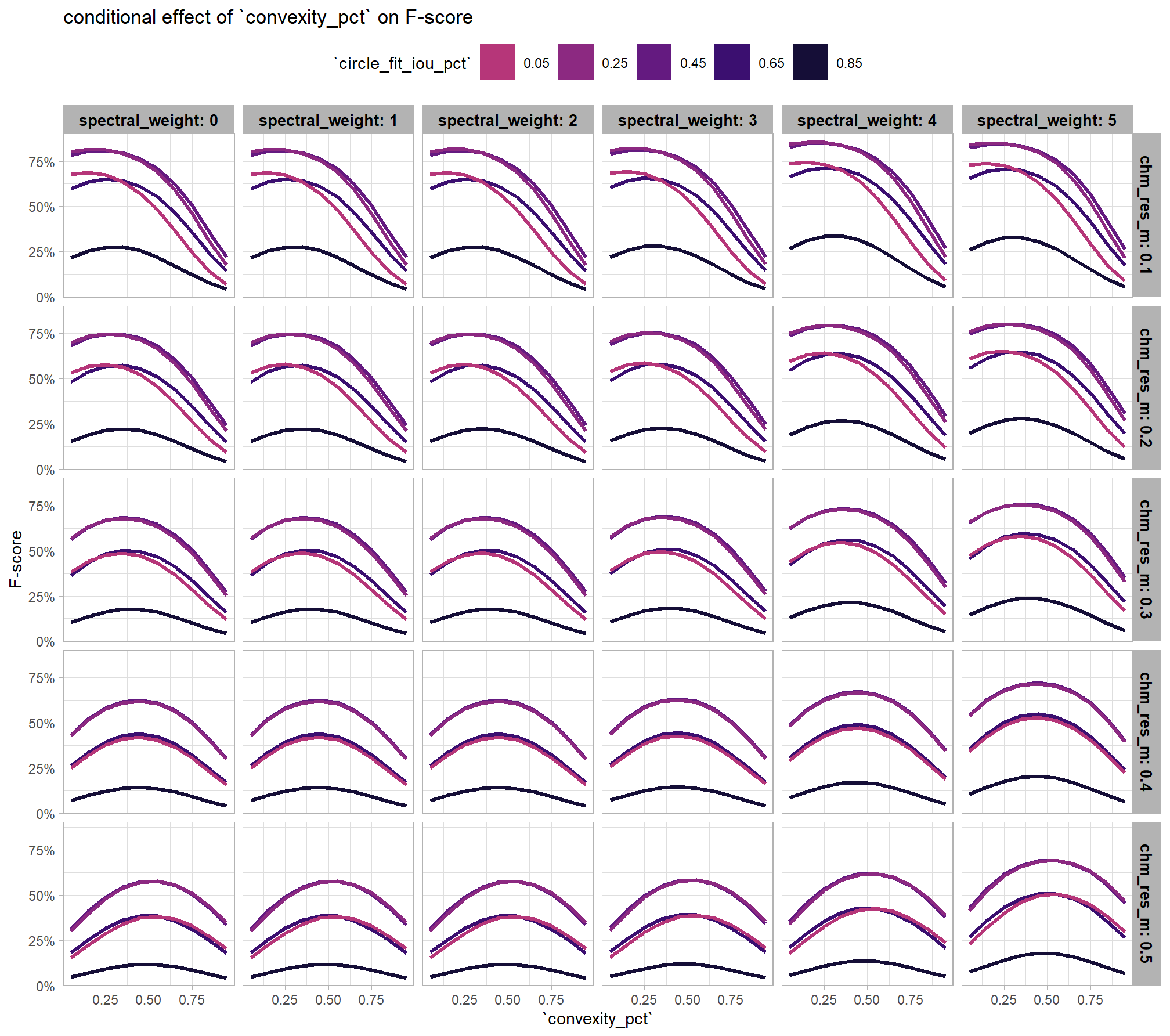
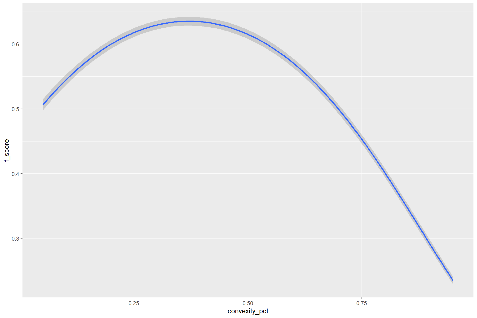
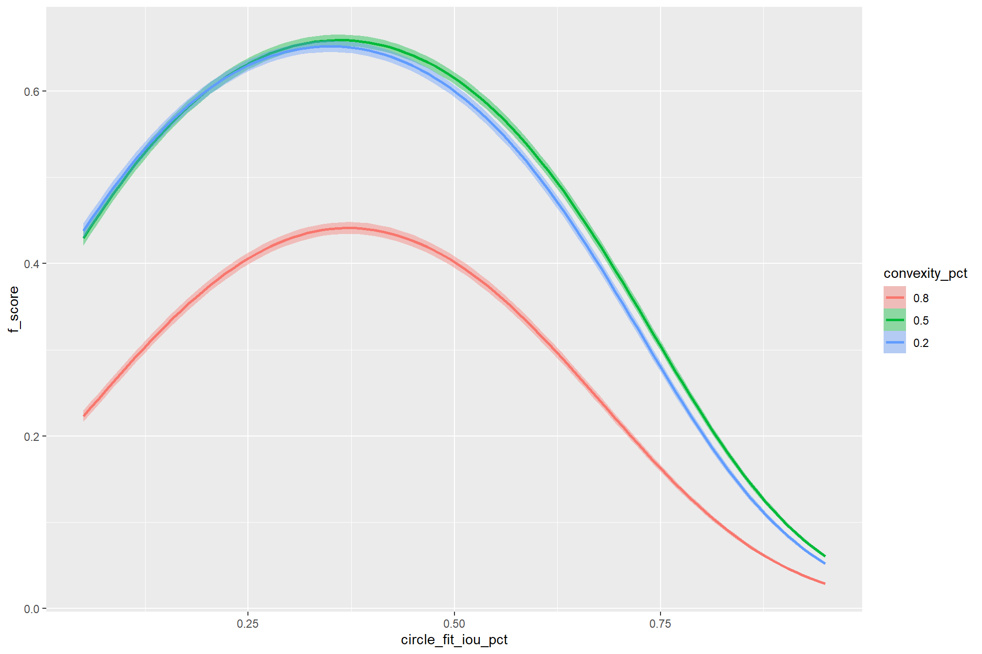
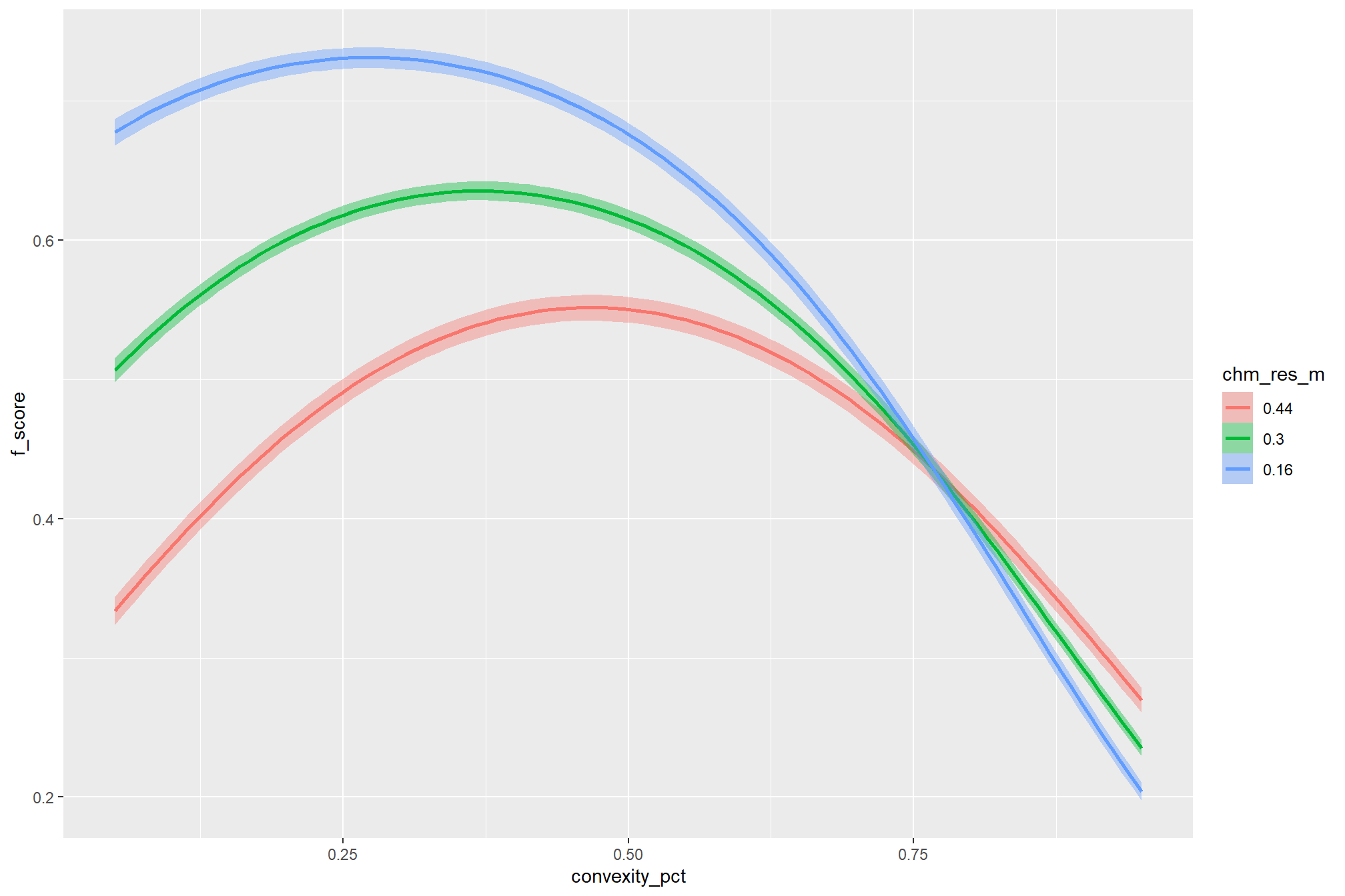
As expected, the model shows that the influence of the convexity_pct parameter on the F-score is conditional on the circle_fit_iou_pct setting. When circle_fit_iou_pct is set too high (requiring nearly perfectly circular pile perimeters), convexity_pct has a minimal impact on the F-score. When circle_fit_iou_pct is set to an optimal value near its vertex (e.g., ~0.25-0.55), the range of convexity_pct values below 0.5 result in the best pile detection for finer resolution CHM data (e.g. < 0.3 m) but for coarser resolution CHM data the optimal convexity_pct setting increases to ~0.37-0.62. Across all CHM resolutions and spectral weighting levels, setting convexity_pct too high (e.g > 0.7) results in steep declines in detection accuracy.
9.1.5.1.3 Optimizing geometric filtering
Given the complexity of our model, which includes a non-linear link function and parameter interactions, calculating the optimal parameter values by solving for them algebraically from the model’s coefficients would be prone to error. instead, we can use a robust Bayesian approach that leverages the model’s posterior predictive distribution. This method is powerful because it inherently accounts for all sources of model uncertainty.
first, we’ll generate a large number of predictions across a fine grid of parameter values (e.g. in steps of 0.01) for each posterior draw of the model coefficients. we’ll generate a large number (e.g. 1000+) of posterior predictive draws for each combination of parameter values. for each posterior predictive draw, we’ll then identify the parameter combination that maximizes the F-score and we’ll be left with a posterior distribution of optimal parameter combinations.
this approach demonstrates a key advantage of the Bayesian framework, allowing us to ask complex questions and find the most probable optimal parameter combination while fully accounting for uncertainty.
# let's get the draws at a very granular level
vertex_draws_temp <-
  tidyr::crossing(
    param_combos_spectral_ranked %>% dplyr::distinct(spectral_weight, spectral_weight_fact)
    , circle_fit_iou_pct = seq(from = 0.0, to = 1, by = 0.01) # very granular to identify vertex
    , convexity_pct = seq(from = 0.0, to = 1, by = 0.01) # very granular to identify vertex
    , chm_res_m = seq(0.1,0.5,by=0.1)
    , max_ht_m = structural_params_settings$max_ht_m
    , max_area_m2 = structural_params_settings$max_area_m2
  ) %>%
  tidybayes::add_epred_draws(brms_f_score_mod, ndraws = 1000, value = "value") %>%
  dplyr::ungroup() %>%
  # for each draw, get the highest f-score by chm_res_m, spectral_weight
  # which we'll use to identify the optimal circle_fit_iou_pct,convexity_pct settings
  # these are essentially "votes" based on likelihood
  dplyr::group_by(
    .draw
    , chm_res_m, spectral_weight
  ) %>%
  dplyr::arrange(desc(value),circle_fit_iou_pct,convexity_pct) %>%
  dplyr::slice(1)
# vertex_draws_temp %>% dplyr::glimpse() # this thing is huge
plot the posterior distribution of optimal parameter setting for circle_fit_iou_pct
vertex_draws_temp %>%
  # dplyr::filter(chm_res_m==0.4) %>%
  dplyr::ungroup() %>%
  ggplot2::ggplot(mapping = ggplot2::aes(x = circle_fit_iou_pct)) +
  tidybayes::stat_dotsinterval(
    point_interval = "median_hdci", .width = c(0.95)
    , quantiles = 100
    , point_size = 3
  ) +
  ggplot2::facet_grid(
    cols = dplyr::vars(spectral_weight)
    , rows = dplyr::vars(chm_res_m)
    , scales = "free_y"
    , labeller = "label_both"
    , axes = "all_x"
  ) +
  # ggplot2::scale_x_continuous(limits = c(0,1)) +
  ggplot2::scale_x_continuous(expand = ggplot2::expansion(mult = 1), breaks = scales::breaks_extended(6)) +
  ggplot2::scale_y_continuous(NULL, breaks = NULL) +
  ggplot2::theme_light() +
  ggplot2::theme(
    strip.text.x = ggplot2::element_text(size = 10, color = "black", face = "bold")
    , strip.text.y = ggplot2::element_text(size = 8, color = "black", face = "bold")
    , axis.text.x = ggplot2::element_text(size = 8)
  )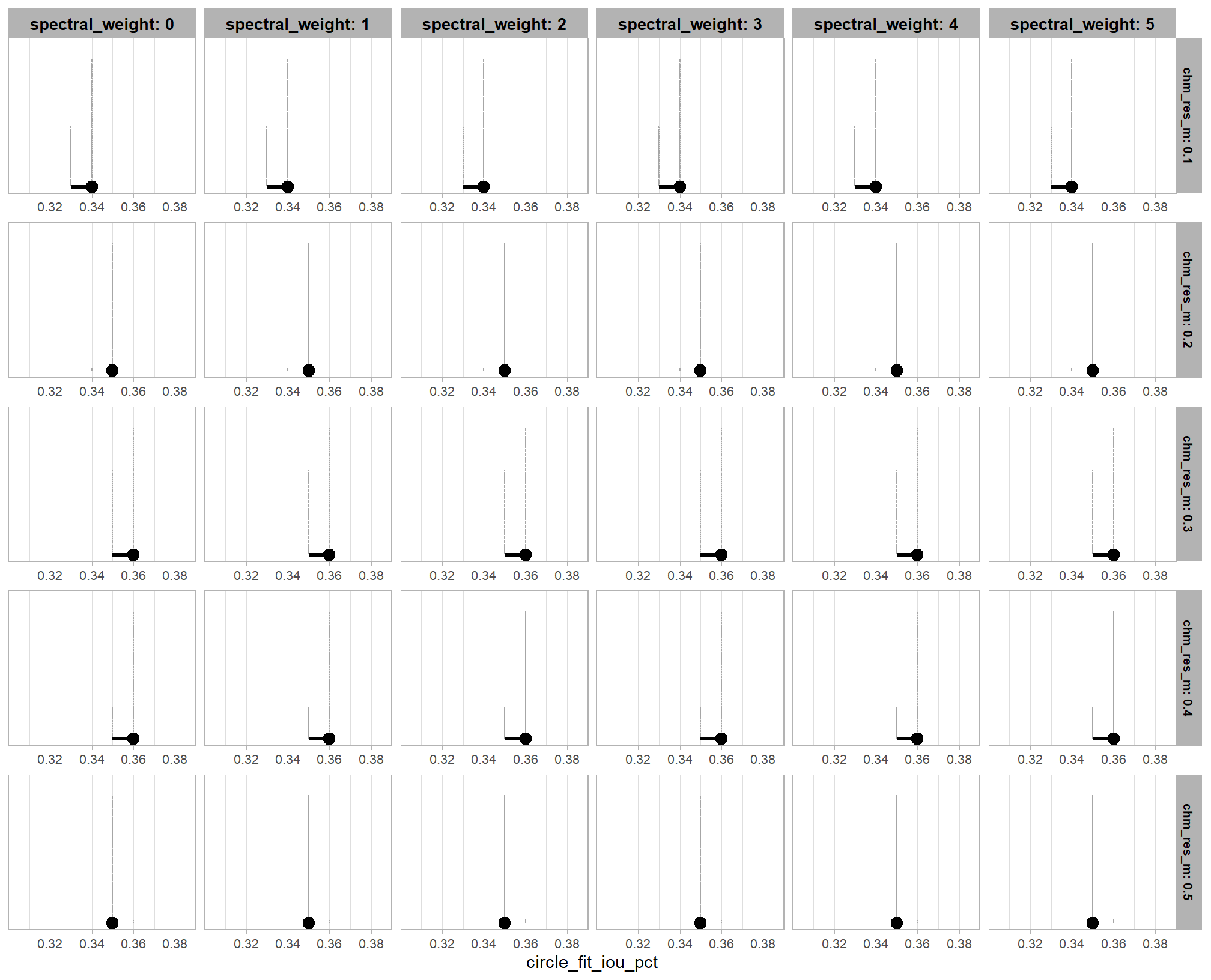
our model is very confident that the optimal circle_fit_iou_pct for maximizing detection accuracy is in a narrow range, just look at that x-axis scale
plot the posterior distribution of optimal parameter setting for convexity_pct
vertex_draws_temp %>%
  dplyr::ungroup() %>%
  ggplot2::ggplot(mapping = ggplot2::aes(x = convexity_pct)) +
  tidybayes::stat_dotsinterval(
    point_interval = "median_hdci", .width = c(0.95)
    , quantiles = 100
    , point_size = 3
  ) +
  ggplot2::facet_grid(
    cols = dplyr::vars(spectral_weight)
    , rows = dplyr::vars(chm_res_m)
    , scales = "free_y"
    , labeller = "label_both"
    , axes = "all_x"
  ) +
  # ggplot2::scale_x_continuous(limits = c(0,1)) +
  ggplot2::scale_x_continuous(expand = ggplot2::expansion(mult = 1), breaks = scales::breaks_extended(6)) +
  ggplot2::scale_y_continuous(NULL, breaks = NULL) +
  ggplot2::theme_light() +
  ggplot2::theme(
    strip.text.x = ggplot2::element_text(size = 10, color = "black", face = "bold")
    , strip.text.y = ggplot2::element_text(size = 8, color = "black", face = "bold")
  )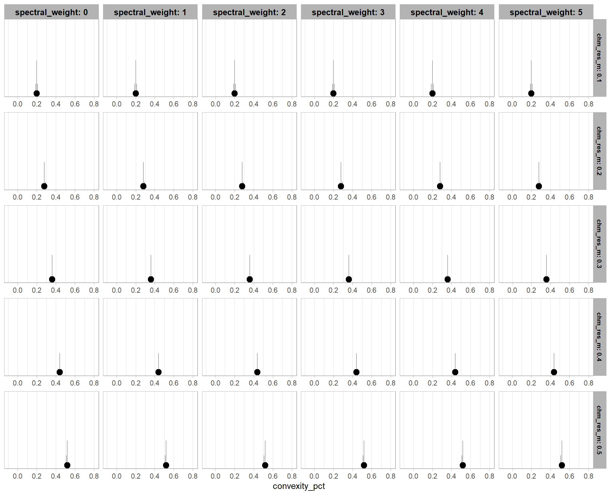
when the circle_fit_iou_pct parameter is optimized, the influence of convexity_pct on detection accuracy is dependent on the CHM resolution. for coarser CHM data (>0.3 m), the model’s predictions indicate with high certainty that the optimal convexity_pct is higher (i.e. requiring more smooth boundaries) than the optimal convexity_pct setting (i.e. requiring less smooth boundaries) for finer resoultion CHM data. this finding is consistent with our previous results and provides additional evidence that the smoothing effect of coarser resolution CHM data makes convexity_pct most effective at filtering irregular objects only when it is set to an intermediate level (e.g. ~0.5).
we can look at this another way, check it
vertex_draws_temp %>%
  dplyr::ungroup() %>%
  ggplot2::ggplot(mapping = ggplot2::aes(y = convexity_pct, x = circle_fit_iou_pct)) +
  # geom_point(alpha=0.2) +
  ggplot2::geom_jitter(alpha=0.2, height = .01, width = .01) +
  ggplot2::facet_grid(
    cols = dplyr::vars(spectral_weight)
    , rows = dplyr::vars(chm_res_m)
    # , scales = "free_y"
    , labeller = "label_both"
    , axes = "all_x"
  ) +
  # ggplot2::scale_x_continuous(limits = c(0,1)) +
  ggplot2::scale_x_continuous(expand = ggplot2::expansion(mult = 1), breaks = scales::breaks_extended(6)) +
  # ggplot2::scale_y_continuous(NULL, breaks = NULL) +
  ggplot2::theme_light() +
  ggplot2::theme(
    strip.text.x = ggplot2::element_text(size = 10, color = "black", face = "bold")
    , strip.text.y = ggplot2::element_text(size = 8, color = "black", face = "bold")
    , axis.text = ggplot2::element_text(size = 8)
  )
note, in the plot above, we slightly “jitter” the points so that they are visible where they would otherwise be stacked on top of each other and only look like a few points instead of the 1000 draws from the posterior we used
let’s table the HDI of the optimal values
# summarize it
table_vertex_draws_temp <- vertex_draws_temp %>%
  dplyr::group_by(
    chm_res_m, spectral_weight
  ) %>%
  dplyr::summarise(
    # get median_hdi
    median_hdi_est_circle_fit_iou_pct = tidybayes::median_hdci(circle_fit_iou_pct)$y
    , median_hdi_lower_circle_fit_iou_pct = tidybayes::median_hdci(circle_fit_iou_pct)$ymin
    , median_hdi_upper_circle_fit_iou_pct = tidybayes::median_hdci(circle_fit_iou_pct)$ymax
    # get median_hdi
    , median_hdi_est_convexity_pct = tidybayes::median_hdci(convexity_pct)$y
    , median_hdi_lower_convexity_pct = tidybayes::median_hdci(convexity_pct)$ymin
    , median_hdi_upper_convexity_pct = tidybayes::median_hdci(convexity_pct)$ymax
  ) %>%
  dplyr::ungroup()
# table it
table_vertex_draws_temp %>%
  kableExtra::kbl(
    digits = 2
    , caption = ""
    , col.names = c(
      "CHM resolution", "spectral_weight"
      , rep(c("median", "HDI low", "HDI high"),2)
    )
    , escape = F
  ) %>%
  kableExtra::kable_styling() %>%
  kableExtra::collapse_rows(columns = 1, valign = "top") %>%
  kableExtra::add_header_above(c(
    " "=2
    , "circle_fit_iou_pct" = 3
    , "convexity_pct" = 3
  )) %>%
kableExtra::scroll_box(height = "8in")| CHM resolution | spectral_weight | median | HDI low | HDI high | median | HDI low | HDI high |
|---|---|---|---|---|---|---|---|
| 0.1 | 0 | 0.34 | 0.33 | 0.34 | 0.20 | 0.19 | 0.21 |
| 1 | 0.34 | 0.33 | 0.34 | 0.20 | 0.19 | 0.21 | |
| 2 | 0.34 | 0.33 | 0.34 | 0.20 | 0.19 | 0.21 | |
| 3 | 0.34 | 0.33 | 0.34 | 0.20 | 0.19 | 0.21 | |
| 4 | 0.34 | 0.33 | 0.34 | 0.20 | 0.19 | 0.21 | |
| 5 | 0.34 | 0.33 | 0.34 | 0.20 | 0.19 | 0.21 | |
| 0.2 | 0 | 0.35 | 0.35 | 0.35 | 0.28 | 0.28 | 0.29 |
| 1 | 0.35 | 0.35 | 0.35 | 0.28 | 0.28 | 0.29 | |
| 2 | 0.35 | 0.35 | 0.35 | 0.28 | 0.28 | 0.29 | |
| 3 | 0.35 | 0.35 | 0.35 | 0.28 | 0.28 | 0.29 | |
| 4 | 0.35 | 0.35 | 0.35 | 0.28 | 0.28 | 0.29 | |
| 5 | 0.35 | 0.35 | 0.35 | 0.28 | 0.28 | 0.29 | |
| 0.3 | 0 | 0.36 | 0.35 | 0.36 | 0.36 | 0.36 | 0.37 |
| 1 | 0.36 | 0.35 | 0.36 | 0.36 | 0.36 | 0.37 | |
| 2 | 0.36 | 0.35 | 0.36 | 0.36 | 0.36 | 0.37 | |
| 3 | 0.36 | 0.35 | 0.36 | 0.36 | 0.36 | 0.37 | |
| 4 | 0.36 | 0.35 | 0.36 | 0.36 | 0.36 | 0.37 | |
| 5 | 0.36 | 0.35 | 0.36 | 0.36 | 0.36 | 0.37 | |
| 0.4 | 0 | 0.36 | 0.35 | 0.36 | 0.44 | 0.43 | 0.44 |
| 1 | 0.36 | 0.35 | 0.36 | 0.44 | 0.43 | 0.44 | |
| 2 | 0.36 | 0.35 | 0.36 | 0.44 | 0.43 | 0.44 | |
| 3 | 0.36 | 0.35 | 0.36 | 0.44 | 0.43 | 0.44 | |
| 4 | 0.36 | 0.35 | 0.36 | 0.44 | 0.43 | 0.44 | |
| 5 | 0.36 | 0.35 | 0.36 | 0.44 | 0.43 | 0.44 | |
| 0.5 | 0 | 0.35 | 0.35 | 0.35 | 0.52 | 0.51 | 0.52 |
| 1 | 0.35 | 0.35 | 0.35 | 0.52 | 0.51 | 0.52 | |
| 2 | 0.35 | 0.35 | 0.35 | 0.52 | 0.51 | 0.52 | |
| 3 | 0.35 | 0.35 | 0.35 | 0.52 | 0.51 | 0.52 | |
| 4 | 0.35 | 0.35 | 0.35 | 0.52 | 0.51 | 0.52 | |
| 5 | 0.35 | 0.35 | 0.35 | 0.52 | 0.51 | 0.52 |
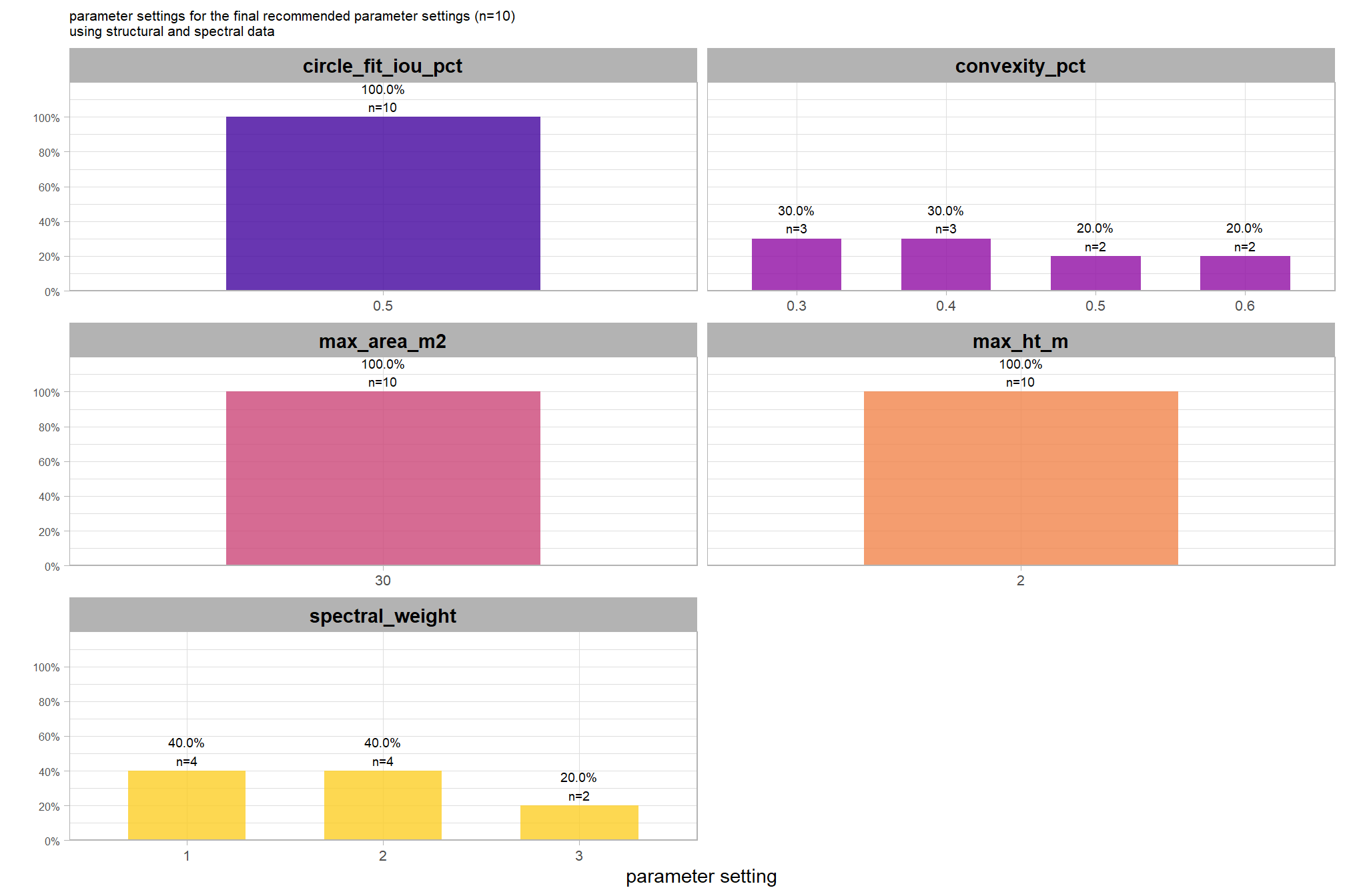
to fix our structural parameter levels so that we can continue to explore the influence of the input data, we’ll select the median of the optimal setting of circle_fit_iou_pct and convexity_pct by CHM resolution levels and spectral weighting. This will result in no one CHM resolution and spectral weighting combination using it’s optimal circle_fit_iou_pct and convexity_pct setting but will provide us with values in the plausible range of optimal settings that work across the CHM resolutions tested with empirical data.
structural_params_settings <-
  vertex_draws_temp %>%
  dplyr::ungroup() %>%
  dplyr::summarise(
    # get median_hdi
    circle_fit_iou_pct = tidybayes::median_hdci(circle_fit_iou_pct)$y
    # , median_hdi_lower_circle_fit_iou_pct = tidybayes::median_hdci(circle_fit_iou_pct)$ymin
    # , median_hdi_upper_circle_fit_iou_pct = tidybayes::median_hdci(circle_fit_iou_pct)$ymax
    # get median_hdi
    , convexity_pct = tidybayes::median_hdci(convexity_pct)$y
    # , median_hdi_lower_convexity_pct = tidybayes::median_hdci(convexity_pct)$ymin
    # , median_hdi_upper_convexity_pct = tidybayes::median_hdci(convexity_pct)$ymax
  ) %>%
  dplyr::bind_cols(
    structural_params_settings
  )
# what?
structural_params_settings %>% dplyr::glimpse()
## Rows: 1
## Columns: 4
## $ circle_fit_iou_pct <dbl> 0.35
## $ convexity_pct <dbl> 0.36
## $ max_ht_m <dbl> 2.3
## $ max_area_m2 <dbl> 469.1.5.2 Input data
to explore the influence of the input data, which includes the presence or absence of spectral data and its weighting (i.e. spectral_weight) as well as the CHM resolution (chm_res_m), we will fix all four structural parameters (max_ht_m, max_area_m2, convexity_pct, circle_fit_iou_pct). the max_ht_m, max_area_m2 parameters will be fixed at expected levels based on the slash pile construction prescription while the convexity_pct, circle_fit_iou_pct will be fixed at the optimal levels determined based on the Bayesian posterior predictive distribution of detection accuracy
we’ll make contrasts of the posterior predictions to probabilistically quantify the influence of the input data (e.g. inclusion of spectral data and it’s weighting and CHM resolution). before we do this we’re going to borrow code from (Tinkham and Woolsey 2024) to make and plot the Bayesian contrasts
############################################
# make the variables for the contrast
############################################
make_contrast_vars <- function(my_data){
my_data %>%
dplyr::mutate(
# get median_hdi
median_hdi_est = tidybayes::median_hdci(value)$y
, median_hdi_lower = tidybayes::median_hdci(value)$ymin
, median_hdi_upper = tidybayes::median_hdci(value)$ymax
# check probability of contrast
, pr_gt_zero = mean(value > 0) %>%
scales::percent(accuracy = 1)
, pr_lt_zero = mean(value < 0) %>%
scales::percent(accuracy = 1)
# check probability that this direction is true
, is_diff_dir = dplyr::case_when(
median_hdi_est >= 0 ~ value > 0
, median_hdi_est < 0 ~ value < 0
)
, pr_diff = mean(is_diff_dir)
# make a label
, pr_diff_lab = dplyr::case_when(
median_hdi_est > 0 ~ paste0(
"Pr("
, stringr::word(contrast, 1, sep = fixed("-")) %>%
stringr::str_squish()
, ">"
, stringr::word(contrast, 2, sep = fixed("-")) %>%
stringr::str_squish()
, ")="
, pr_diff %>% scales::percent(accuracy = 1)
)
, median_hdi_est < 0 ~ paste0(
"Pr("
, stringr::word(contrast, 2, sep = fixed("-")) %>%
stringr::str_squish()
, ">"
, stringr::word(contrast, 1, sep = fixed("-")) %>%
stringr::str_squish()
, ")="
, pr_diff %>% scales::percent(accuracy = 1)
)
)
# make a SMALLER label
, pr_diff_lab_sm = dplyr::case_when(
median_hdi_est >= 0 ~ paste0(
"Pr(>0)="
, pr_diff %>% scales::percent(accuracy = 1)
)
, median_hdi_est < 0 ~ paste0(
"Pr(<0)="
, pr_diff %>% scales::percent(accuracy = 1)
)
)
, pr_diff_lab_pos = dplyr::case_when(
median_hdi_est > 0 ~ median_hdi_upper
, median_hdi_est < 0 ~ median_hdi_lower
) * 1.075
, sig_level = dplyr::case_when(
pr_diff > 0.99 ~ 0
, pr_diff > 0.95 ~ 1
, pr_diff > 0.9 ~ 2
, pr_diff > 0.8 ~ 3
, T ~ 4
) %>%
factor(levels = c(0:4), labels = c(">99%","95%","90%","80%","<80%"), ordered = T)
)
}
############################################
# plot the contrast
############################################
plt_contrast <- function(
my_data
, x = "value"
, y = "contrast"
, fill = "pr_diff"
, label = "pr_diff_lab"
, label_pos = "pr_diff_lab_pos"
, label_size = 3
, x_expand = c(0.1, 0.1)
, facet = NA
, y_axis_title = ""
, x_axis_title = "difference"
, caption_text = "" # form_temp
, annotate_size = 2.2
, annotate_which = "both" # "both", "left", "right"
, include_zero = T
) {
# df for annotation
get_annotation_df <- function(
my_text_list = c(
"Bottom Left (h0,v0)","Top Left (h0,v1)"
,"Bottom Right h1,v0","Top Right h1,v1"
)
, hjust = c(0,0,1,1) # higher values = right, lower values = left
, vjust = c(0,1.3,0,1.3) # higher values = down, lower values = up
){
df = data.frame(
xpos = c(-Inf,-Inf,Inf,Inf)
, ypos = c(-Inf, Inf,-Inf,Inf)
, annotate_text = my_text_list
, hjustvar = hjust
, vjustvar = vjust
)
return(df)
}
if(annotate_which=="left"){
text_list <- c(
"","L.H.S. < R.H.S."
,"",""
)
}else if(annotate_which=="right"){
text_list <- c(
"",""
,"","L.H.S. > R.H.S."
)
}else{
text_list <- c(
"","L.H.S. < R.H.S."
,"","L.H.S. > R.H.S."
)
}
# plot base
plt <-
my_data %>%
ggplot(aes(x = .data[[x]], y = .data[[y]]))
if(include_zero){
plt <- plt + geom_vline(xintercept = 0, linetype = "solid", color = "gray33", lwd = 1.1)
}
# plot meat
plt <- plt +
tidybayes::stat_halfeye(
mapping = aes(fill = .data[[fill]])
, point_interval = median_hdi, .width = c(0.5,0.95)
# , slab_fill = "gray22", slab_alpha = 1
, interval_color = "black", point_color = "black", point_fill = "black"
, point_size = 0.9
, justification = -0.01
) +
geom_text(
data = get_annotation_df(
my_text_list = text_list
)
, mapping = aes(
x = xpos, y = ypos
, hjust = hjustvar, vjust = vjustvar
, label = annotate_text
, fontface = "bold"
)
, size = annotate_size
, color = "gray30" # "#2d2a4d" #"#204445"
) +
# scale_fill_fermenter(
# n.breaks = 5 # 10 use 10 if can go full range 0-1
# , palette = "PuOr" # "RdYlBu"
# , direction = 1
# , limits = c(0.5,1) # use c(0,1) if can go full range 0-1
# , labels = scales::percent
# ) +
scale_fill_stepsn(
n.breaks = 5 # 10 use 10 if can go full range 0-1
, colors = harrypotter::hp(n=5, option="ravenclaw", direction = -1) # RColorBrewer::brewer.pal(11,"PuOr")[c(3,4,8,10,11)]
, limits = c(0.5,1) # use c(0,1) if can go full range 0-1
, labels = scales::percent
) +
scale_x_continuous(expand = expansion(mult = x_expand)) +
labs(
y = y_axis_title
, x = x_axis_title
, fill = "Pr(contrast)"
, subtitle = "posterior predictive distribution of group constrasts with 95% & 50% HDI"
, caption = caption_text
) +
theme_light() +
theme(
legend.text = element_text(size = 7)
, legend.title = element_text(size = 8)
, axis.text.x = element_text(angle = 90, vjust = 0.5, hjust = 1.05)
, strip.text = element_text(color = "black", face = "bold")
) +
guides(fill = guide_colorbar(theme = theme(
legend.key.width = unit(1, "lines"),
legend.key.height = unit(12, "lines")
)))
# label or not
if(!is.na(label) && !is.na(label_pos) && !is.na(label_size)){
plt <- plt +
geom_text(
data = my_data %>%
dplyr::filter(pr_diff_lab_pos>=0) %>%
dplyr::ungroup() %>%
dplyr::select(tidyselect::all_of(c(
y
, fill
, label
, label_pos
, facet
))) %>%
dplyr::distinct()
, mapping = aes(x = .data[[label_pos]], label = .data[[label]])
, vjust = -1, hjust = 0, size = label_size
) +
geom_text(
data = my_data %>%
dplyr::filter(pr_diff_lab_pos<0) %>%
dplyr::ungroup() %>%
dplyr::select(tidyselect::all_of(c(
y
, fill
, label
, label_pos
, facet
))) %>%
dplyr::distinct()
, mapping = aes(x = .data[[label_pos]], label = .data[[label]])
, vjust = -1, hjust = +1, size = label_size
)
}
# return facet or not
if(max(is.na(facet))==0){
return(
plt +
facet_grid(cols = vars(.data[[facet]]))
)
}
else{return(plt)}
}now get the posterior predictive draws
draws_temp <-
tidyr::crossing(
structural_params_settings
, param_combos_spectral_ranked %>% dplyr::distinct(spectral_weight_fact, spectral_weight)
, param_combos_spectral_ranked %>% dplyr::distinct(chm_res_m)
) %>%
tidybayes::add_epred_draws(brms_f_score_mod, ndraws = 1111) %>%
dplyr::rename(value = .epred)
# # huh?
draws_temp %>% dplyr::glimpse()## Rows: 33,330
## Columns: 12
## Groups: circle_fit_iou_pct, convexity_pct, max_ht_m, max_area_m2, spectral_weight_fact, spectral_weight, chm_res_m, .row [30]
## $ circle_fit_iou_pct <dbl> 0.35, 0.35, 0.35, 0.35, 0.35, 0.35, 0.35, 0.35, 0…
## $ convexity_pct <dbl> 0.36, 0.36, 0.36, 0.36, 0.36, 0.36, 0.36, 0.36, 0…
## $ max_ht_m <dbl> 2.3, 2.3, 2.3, 2.3, 2.3, 2.3, 2.3, 2.3, 2.3, 2.3,…
## $ max_area_m2 <dbl> 46, 46, 46, 46, 46, 46, 46, 46, 46, 46, 46, 46, 4…
## $ spectral_weight_fact <fct> structural only, structural only, structural only…
## $ spectral_weight <fct> 0, 0, 0, 0, 0, 0, 0, 0, 0, 0, 0, 0, 0, 0, 0, 0, 0…
## $ chm_res_m <dbl> 0.1, 0.1, 0.1, 0.1, 0.1, 0.1, 0.1, 0.1, 0.1, 0.1,…
## $ .row <int> 1, 1, 1, 1, 1, 1, 1, 1, 1, 1, 1, 1, 1, 1, 1, 1, 1…
## $ .chain <int> NA, NA, NA, NA, NA, NA, NA, NA, NA, NA, NA, NA, N…
## $ .iteration <int> NA, NA, NA, NA, NA, NA, NA, NA, NA, NA, NA, NA, N…
## $ .draw <int> 1, 2, 3, 4, 5, 6, 7, 8, 9, 10, 11, 12, 13, 14, 15…
## $ value <dbl> 0.8102877, 0.8088862, 0.8099895, 0.8118048, 0.811…9.1.5.2.1 CHM resolution
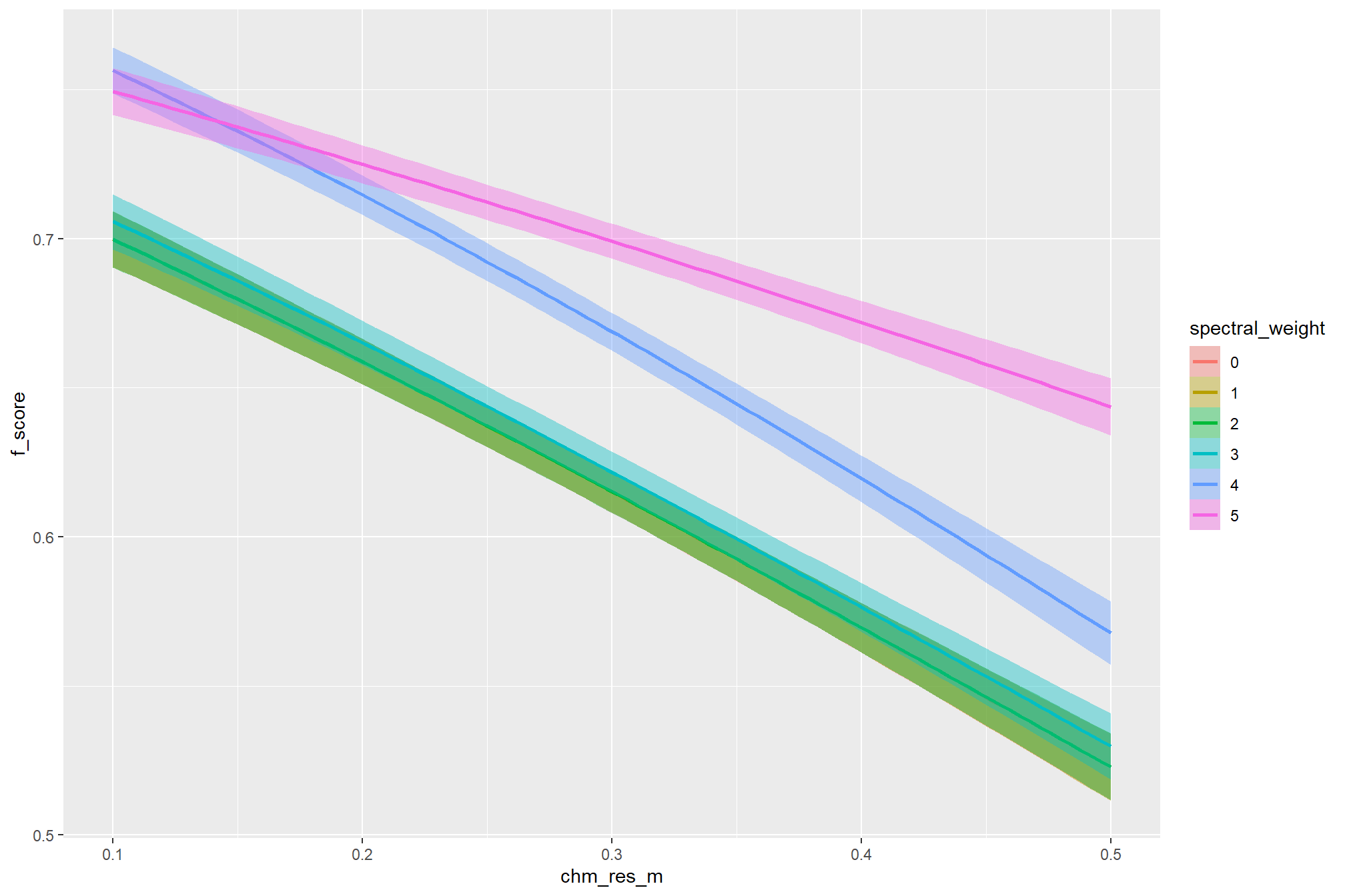
first, we’ll look at the impact of changing CHM resolution by the spectral_weight parameter where a value of “0” indicates no spectral data was used (i.e. structural only), the lowest weighting of the spectral data is “1” (only one spectral index threshold must be met), and the highest weighting of spectral data is “5” (all spectral index thresholds must be met).
our questions regarding CHM resolution were:
- question 1: does CHM resolution influences detection accuracy?
- question 2: does the effect of CHM resolution change based on the inclusion of spectral data versus using only structural data?
we can answer those questions using our model by considering the credible slope of the CHM resolution predictor as a function of the spectral_weight parameter (e.g. Kurz 2025; Kruschke (2015, Ch. 18))
pal_spectral_weight <- c("gray77", harrypotter::hp(n=5, option = "gryffindor", direction = 1)) # %>% scales::show_col()
# brms::posterior_summary(brms_f_score_mod)
draws_temp %>%
ggplot2::ggplot(mapping = ggplot2::aes(x = chm_res_m, y = value, color = spectral_weight)) +
# tidybayes::stat_halfeye() +
tidybayes::stat_lineribbon(point_interval = "median_hdi", .width = c(0.95)) +
# ggplot2::facet_wrap(facets = dplyr::vars(spectral_weight))
ggplot2::scale_fill_brewer(palette = "Greys") +
ggplot2::scale_color_manual(values = pal_spectral_weight) +
ggplot2::scale_y_continuous(labels = scales::percent) +
ggplot2::labs(x = "CHM resolution", y = "F-score") +
ggplot2::theme_light() +
ggplot2::theme(
legend.position = "top"
) +
ggplot2::guides(
color = ggplot2::guide_legend(override.aes = list(shape = 15, lwd = 8, fill = NA))
, fill = "none"
)
there are a few takeaways from this plot:
- including spectral data and setting the
spectral_weightto “1”, “2”, or “3” appears to be not much different than not including spectral data at all (but we’ll probabilistically test this later on) - including spectral data and setting the
spectral_weightto “4” yields a larger negative impact of decreasing CHM resolution on detection accuracy - including spectral data and setting the
spectral_weightto “5” yields a smaller negative impact of decreasing CHM resolution on detection accuracy and beyond a CHM resolution of ~0.13 m, detection accuracy is maximized when setting thespectral_weightto “5”. this makes intuitive sense because as the structural information about slash piles becomes less fine grain (i.e. more coarse), we should put more weight into the spectral data for detecting slash piles
all of this is to say that the impact of CHM resolution varies based on the spectral_weight setting and vice-versa
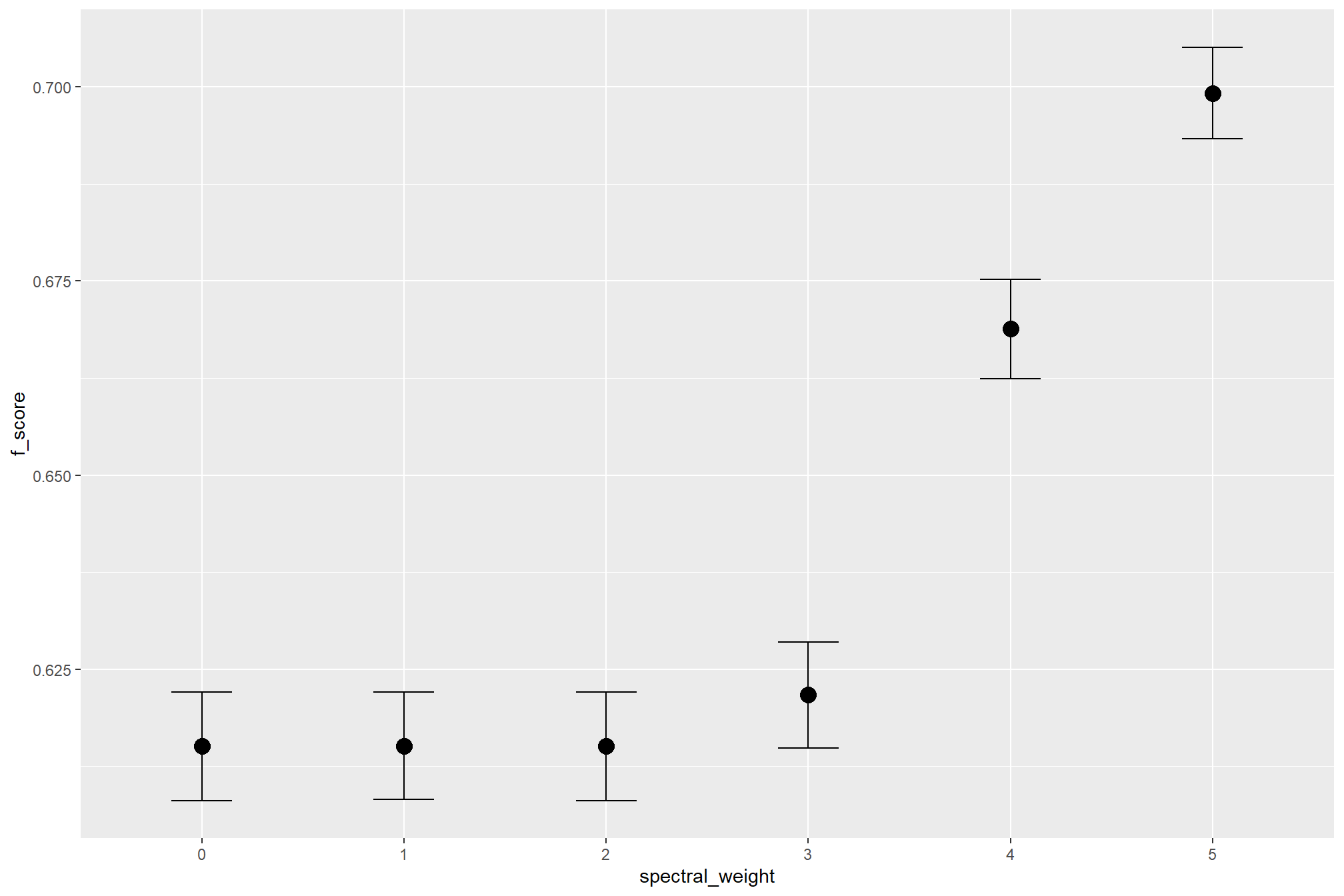
averaging across all other parameters to look at the main effect of including spectral data with the spectral_weight parameter, these results align with what we saw during our data summarization exploration: increasing the spectral_weight (where “5” requires all spectral index thresholds to be met) had minimal impact on metrics until a value of “3”, at which point F-score saw a minimal increase; at a spectral_weight of “4”, the F-score significantly improved, but at a value of “5” F-score was lower than not including the spectral data at all when CHM resolution was fine (e.g. <0.3) but for coarse resolution CHM data the spectral data became more important for detection accuracy.
let’s test including predictions at CHM resolutions outside of the bounds of the data tested (e.g. > 0.5 m resolution)
tidyr::crossing(
structural_params_settings
, param_combos_spectral_ranked %>% dplyr::distinct(spectral_weight_fact, spectral_weight)
, chm_res_m = seq(0.05,1,by = 0.05)
) %>%
tidybayes::add_epred_draws(brms_f_score_mod, ndraws = 1111) %>%
dplyr::rename(value = .epred) %>%
ggplot2::ggplot(mapping = ggplot2::aes(x = chm_res_m, y = value, color = spectral_weight)) +
# tidybayes::stat_halfeye() +
tidybayes::stat_lineribbon(point_interval = "median_hdi", .width = c(0.95)) +
# ggplot2::facet_wrap(facets = dplyr::vars(spectral_weight))
ggplot2::scale_fill_brewer(palette = "Greys") +
ggplot2::scale_color_manual(values = pal_spectral_weight) +
ggplot2::scale_y_continuous(labels = scales::percent) +
ggplot2::scale_x_continuous(breaks = scales::breaks_extended(n=8)) +
ggplot2::labs(x = "CHM resolution", y = "F-score") +
ggplot2::theme_light() +
ggplot2::theme(
legend.position = "top"
) +
ggplot2::guides(
color = ggplot2::guide_legend(override.aes = list(shape = 15, lwd = 8, fill = NA))
, fill = "none"
)
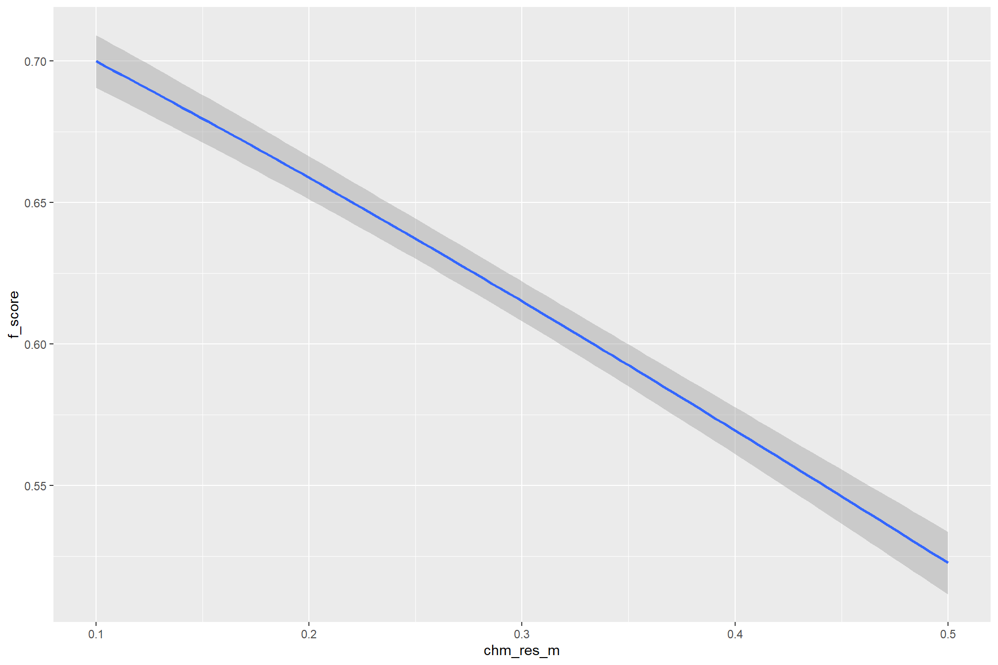
even at the coarse CHM resolutions not represented in the data, the model is still confident that coarser resolution CHM data decreases detection accuracy
we can look at the posterior distributions of the expected F-score at different CHM resolution levels by the inclusion (or exclusion) of spectral data and it’s weighting
draws_temp %>%
ggplot2::ggplot(mapping = ggplot2::aes(y=value, x=chm_res_m)) +
tidybayes::stat_eye(
mapping = ggplot2::aes(fill = spectral_weight)
, point_interval = median_hdi, .width = .95
, slab_alpha = 0.95
, interval_color = "gray44", linewidth = 1
, point_color = "gray44", point_fill = "gray44", point_size = 1
) +
ggplot2::facet_grid(cols = dplyr::vars(spectral_weight), labeller = "label_both") +
ggplot2::scale_fill_manual(values = pal_spectral_weight) +
ggplot2::scale_y_continuous(limits = c(0,NA), labels = scales::percent, breaks = scales::breaks_extended(16)) +
ggplot2::labs(x = "CHM resolution", y = "F-score") +
ggplot2::theme_light() +
ggplot2::theme(
legend.position = "none"
, strip.text = ggplot2::element_text(size = 8, color = "black", face = "bold")
)
table that
draws_temp %>%
dplyr::mutate(spectral_weight = forcats::fct_relabel(spectral_weight,~paste0("spectral_weight: ", .x, recycle0 = T))) %>%
dplyr::group_by(spectral_weight, chm_res_m) %>%
dplyr::summarise(
# get median_hdi
median_hdi_est = tidybayes::median_hdci(value)$y
, median_hdi_lower = tidybayes::median_hdci(value)$ymin
, median_hdi_upper = tidybayes::median_hdci(value)$ymax
) %>%
dplyr::ungroup() %>%
dplyr::arrange(spectral_weight, chm_res_m) %>%
# format pcts
dplyr::mutate(dplyr::across(
tidyselect::starts_with("median_hdi_")
, ~ scales::percent(.x, accuracy = 0.1)
)) %>%
kableExtra::kbl(
digits = 2
, caption = "F-score<br>95% HDI of the posterior predictive distribution"
, col.names = c(
"spectral_weight", "CHM resolution"
, c("F-score<br>median", "HDI low", "HDI high")
)
, escape = F
) %>%
kableExtra::kable_styling() %>%
kableExtra::collapse_rows(columns = 1, valign = "top") %>%
kableExtra::scroll_box(height = "8in")| spectral_weight | CHM resolution |
F-score median |
HDI low | HDI high |
|---|---|---|---|---|
| spectral_weight: 0 | 0.1 | 80.9% | 80.2% | 81.5% |
| 0.2 | 76.0% | 75.3% | 76.6% | |
| 0.3 | 70.3% | 69.7% | 70.9% | |
| 0.4 | 63.9% | 63.1% | 64.7% | |
| 0.5 | 57.0% | 55.8% | 58.1% | |
| spectral_weight: 1 | 0.1 | 80.9% | 80.2% | 81.6% |
| 0.2 | 76.0% | 75.4% | 76.7% | |
| 0.3 | 70.3% | 69.7% | 71.0% | |
| 0.4 | 63.9% | 63.1% | 64.7% | |
| 0.5 | 57.0% | 55.9% | 58.1% | |
| spectral_weight: 2 | 0.1 | 80.9% | 80.2% | 81.6% |
| 0.2 | 76.0% | 75.4% | 76.7% | |
| 0.3 | 70.3% | 69.6% | 70.9% | |
| 0.4 | 63.9% | 63.1% | 64.8% | |
| 0.5 | 57.0% | 55.8% | 58.1% | |
| spectral_weight: 3 | 0.1 | 81.3% | 80.7% | 82.1% |
| 0.2 | 76.5% | 76.0% | 77.3% | |
| 0.3 | 70.9% | 70.3% | 71.5% | |
| 0.4 | 64.6% | 63.8% | 65.4% | |
| 0.5 | 57.7% | 56.4% | 58.7% | |
| spectral_weight: 4 | 0.1 | 84.9% | 84.3% | 85.5% |
| 0.2 | 80.4% | 79.9% | 80.9% | |
| 0.3 | 74.9% | 74.4% | 75.6% | |
| 0.4 | 68.5% | 67.8% | 69.3% | |
| 0.5 | 61.4% | 60.2% | 62.4% | |
| spectral_weight: 5 | 0.1 | 84.4% | 84.0% | 85.0% |
| 0.2 | 81.2% | 80.8% | 81.7% | |
| 0.3 | 77.5% | 77.0% | 78.0% | |
| 0.4 | 73.3% | 72.6% | 73.9% | |
| 0.5 | 68.6% | 67.6% | 69.5% |
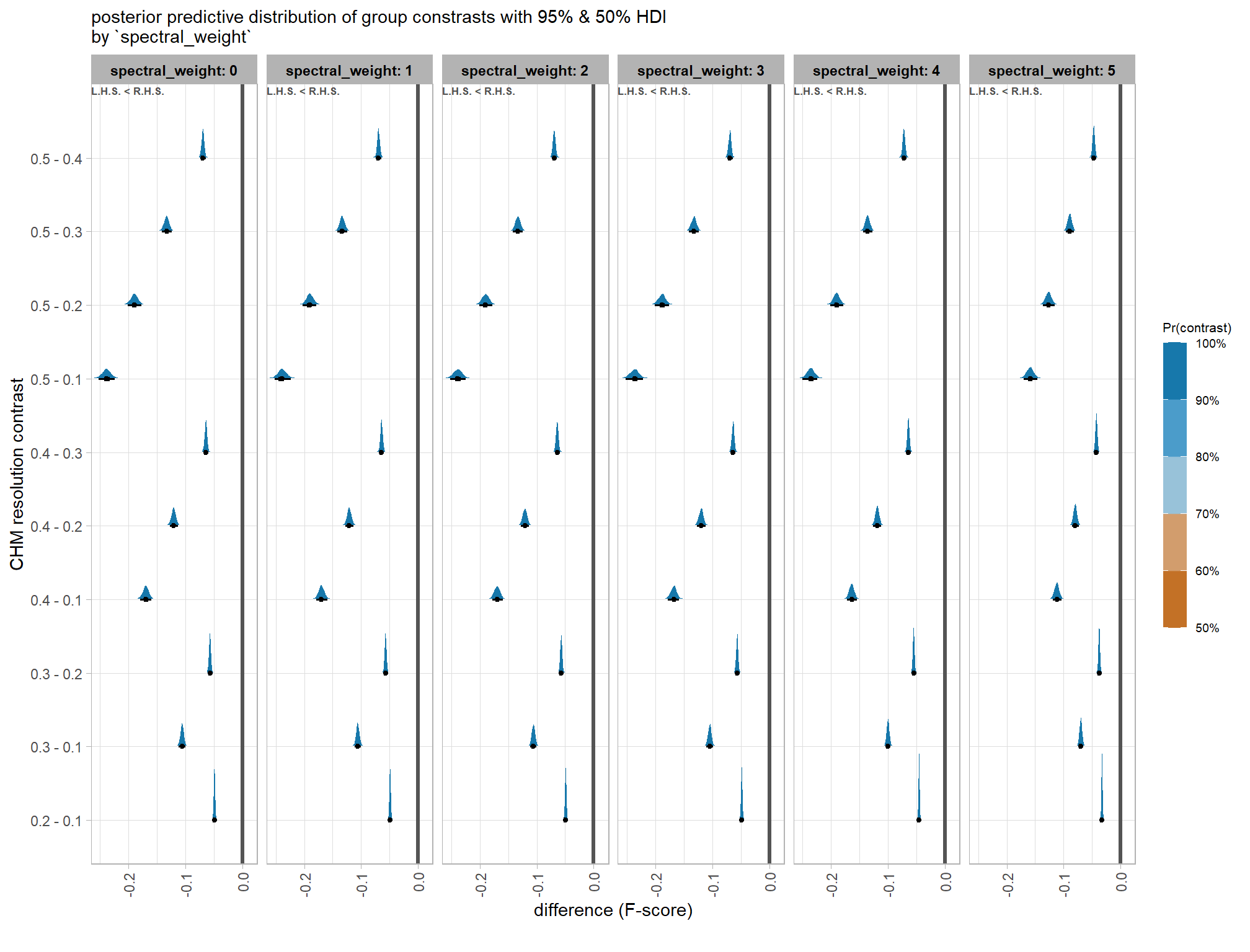
now we’ll probabilistically test the hypothesis that coarser resolution CHM data results in lower detection accuracy and quantify by how much. we’ll look at the influence of CHM resolution based on the inclusion of spectral data (or exclusion) and it’s weighting determined by the spectral_weight parameter
contrast_temp <-
draws_temp %>%
dplyr::filter(
round(chm_res_m,2) == round(chm_res_m,1) # let's just look at every 0.1 m (10 cm)
) %>%
dplyr::group_by(spectral_weight) %>%
tidybayes::compare_levels(
value
, by = chm_res_m
, comparison =
# "control"
# tidybayes::emmeans_comparison("revpairwise")
"pairwise"
) %>%
# dplyr::glimpse()
dplyr::rename(contrast = chm_res_m) %>%
# group the data before calculating contrast variables %>%
dplyr::group_by(spectral_weight, contrast) %>%
make_contrast_vars() %>%
# relabel the label for the facets
dplyr::mutate(spectral_weight = forcats::fct_relabel(spectral_weight,~paste0("spectral_weight: ", .x, recycle0 = T)))
# huh?
# contrast_temp %>% dplyr::glimpse()
# plot it
plt_contrast(
contrast_temp
# , caption_text = form_temp
, y_axis_title = "CHM resolution contrast"
, x_axis_title = "difference (F-score)"
, facet = "spectral_weight"
, label_size = NA
, x_expand = c(0,0.1)
, annotate_which = "left"
) +
labs(
subtitle = "posterior predictive distribution of group constrasts with 95% & 50% HDI\nby `spectral_weight`"
)
let’s table it
contrast_temp %>%
dplyr::distinct(
spectral_weight, contrast
, median_hdi_est, median_hdi_lower, median_hdi_upper
, pr_lt_zero # , pr_gt_zero
) %>%
dplyr::arrange(spectral_weight, contrast) %>%
# format pcts
dplyr::mutate(dplyr::across(
tidyselect::starts_with("median_hdi_")
, ~ scales::percent(.x, accuracy = 0.1)
)) %>%
kableExtra::kbl(
digits = 2
, caption = "brms::brm model: 95% HDI of the posterior predictive distribution of group constrasts"
, col.names = c(
"spectral_weight", "CHM res. contrast"
, "difference (F-score)"
, "HDI low", "HDI high"
, "Pr(diff<0)"
)
, escape = F
) %>%
kableExtra::kable_styling() %>%
kableExtra::collapse_rows(columns = 1, valign = "top") %>%
kableExtra::scroll_box(height = "8in")| spectral_weight | CHM res. contrast | difference (F-score) | HDI low | HDI high | Pr(diff<0) |
|---|---|---|---|---|---|
| spectral_weight: 0 | 0.2 - 0.1 | -4.9% | -5.1% | -4.7% | 100% |
| 0.3 - 0.1 | -10.6% | -11.2% | -10.0% | 100% | |
| 0.3 - 0.2 | -5.7% | -6.0% | -5.4% | 100% | |
| 0.4 - 0.1 | -17.0% | -17.9% | -16.0% | 100% | |
| 0.4 - 0.2 | -12.1% | -12.8% | -11.3% | 100% | |
| 0.4 - 0.3 | -6.4% | -6.8% | -6.0% | 100% | |
| 0.5 - 0.1 | -23.9% | -25.3% | -22.4% | 100% | |
| 0.5 - 0.2 | -19.0% | -20.2% | -17.8% | 100% | |
| 0.5 - 0.3 | -13.3% | -14.1% | -12.4% | 100% | |
| 0.5 - 0.4 | -6.9% | -7.3% | -6.4% | 100% | |
| spectral_weight: 1 | 0.2 - 0.1 | -4.9% | -5.1% | -4.6% | 100% |
| 0.3 - 0.1 | -10.6% | -11.1% | -10.0% | 100% | |
| 0.3 - 0.2 | -5.7% | -6.0% | -5.3% | 100% | |
| 0.4 - 0.1 | -17.0% | -17.8% | -15.9% | 100% | |
| 0.4 - 0.2 | -12.1% | -12.8% | -11.3% | 100% | |
| 0.4 - 0.3 | -6.4% | -6.8% | -6.0% | 100% | |
| 0.5 - 0.1 | -23.9% | -25.2% | -22.4% | 100% | |
| 0.5 - 0.2 | -19.0% | -20.2% | -17.8% | 100% | |
| 0.5 - 0.3 | -13.3% | -14.1% | -12.4% | 100% | |
| 0.5 - 0.4 | -6.9% | -7.3% | -6.4% | 100% | |
| spectral_weight: 2 | 0.2 - 0.1 | -4.9% | -5.1% | -4.7% | 100% |
| 0.3 - 0.1 | -10.6% | -11.1% | -10.0% | 100% | |
| 0.3 - 0.2 | -5.7% | -6.0% | -5.3% | 100% | |
| 0.4 - 0.1 | -17.0% | -17.9% | -16.0% | 100% | |
| 0.4 - 0.2 | -12.1% | -12.8% | -11.3% | 100% | |
| 0.4 - 0.3 | -6.4% | -6.8% | -6.0% | 100% | |
| 0.5 - 0.1 | -23.9% | -25.2% | -22.5% | 100% | |
| 0.5 - 0.2 | -19.0% | -20.1% | -17.8% | 100% | |
| 0.5 - 0.3 | -13.3% | -14.2% | -12.5% | 100% | |
| 0.5 - 0.4 | -6.9% | -7.4% | -6.5% | 100% | |
| spectral_weight: 3 | 0.2 - 0.1 | -4.8% | -5.1% | -4.6% | 100% |
| 0.3 - 0.1 | -10.4% | -11.0% | -9.9% | 100% | |
| 0.3 - 0.2 | -5.6% | -6.0% | -5.3% | 100% | |
| 0.4 - 0.1 | -16.8% | -17.8% | -15.8% | 100% | |
| 0.4 - 0.2 | -12.0% | -12.7% | -11.2% | 100% | |
| 0.4 - 0.3 | -6.3% | -6.8% | -5.9% | 100% | |
| 0.5 - 0.1 | -23.7% | -25.2% | -22.2% | 100% | |
| 0.5 - 0.2 | -18.8% | -20.1% | -17.6% | 100% | |
| 0.5 - 0.3 | -13.2% | -14.1% | -12.4% | 100% | |
| 0.5 - 0.4 | -6.9% | -7.4% | -6.4% | 100% | |
| spectral_weight: 4 | 0.2 - 0.1 | -4.5% | -4.7% | -4.3% | 100% |
| 0.3 - 0.1 | -10.0% | -10.5% | -9.5% | 100% | |
| 0.3 - 0.2 | -5.5% | -5.8% | -5.2% | 100% | |
| 0.4 - 0.1 | -16.4% | -17.2% | -15.5% | 100% | |
| 0.4 - 0.2 | -11.9% | -12.6% | -11.3% | 100% | |
| 0.4 - 0.3 | -6.4% | -6.8% | -6.0% | 100% | |
| 0.5 - 0.1 | -23.6% | -25.0% | -22.4% | 100% | |
| 0.5 - 0.2 | -19.0% | -20.1% | -17.9% | 100% | |
| 0.5 - 0.3 | -13.6% | -14.4% | -12.7% | 100% | |
| 0.5 - 0.4 | -7.2% | -7.6% | -6.7% | 100% | |
| spectral_weight: 5 | 0.2 - 0.1 | -3.2% | -3.4% | -3.0% | 100% |
| 0.3 - 0.1 | -6.9% | -7.4% | -6.5% | 100% | |
| 0.3 - 0.2 | -3.7% | -4.0% | -3.4% | 100% | |
| 0.4 - 0.1 | -11.2% | -11.9% | -10.3% | 100% | |
| 0.4 - 0.2 | -7.9% | -8.5% | -7.3% | 100% | |
| 0.4 - 0.3 | -4.2% | -4.5% | -3.9% | 100% | |
| 0.5 - 0.1 | -15.9% | -17.0% | -14.6% | 100% | |
| 0.5 - 0.2 | -12.6% | -13.6% | -11.6% | 100% | |
| 0.5 - 0.3 | -8.9% | -9.6% | -8.1% | 100% | |
| 0.5 - 0.4 | -4.7% | -5.1% | -4.3% | 100% |
it is clear from these contrasts that coarser CHM resolutions lead to a decrease in detection accuracy. without the inclusion of spectral data (i.e. spectral_weight = “0”), a 0.1 m increase in CHM resolution coarseness results in an approximate decrease in F-score of ~5-7 percentage points. for example, the expected F-score decreases from 72% to 66% when moving from a 0.2 m resolution CHM raster to a 0.3 m raster, respectively.
when spectral data is included, this trend of decreasing accuracy with coarser resolution persists, but there is a greater improvement in detection accuracy at coarser resolutions when making the resolution more granular. for example, when including spectral data and setting the spectral_weight parameter to “4” (i.e., requiring four spectral thresholds to be met), a shift from a 0.5 m resolution raster to a 0.3 m raster results in a substantial F-score increase of 14.5 percentage points, from 57% to 71%.
9.1.5.2.2 Spectral data
now we’ll look at the impact of including (or excluding) spectral data and the weighting of the spectral_weight parameter where a value of “0” indicates no spectral data was used (i.e. structural only), the lowest weighting of the spectral data is “1” (only one spectral index threshold must be met), and the highest weighting of spectral data is “5” (all spectral index thresholds must be met).
# viridis::rocket(5, begin = 0.9, end = 0.6) %>% scales::show_col()
# brms::posterior_summary(brms_f_score_mod)
draws_temp %>%
dplyr::filter(
round(chm_res_m,2) == round(chm_res_m,1) # let's just look at every 0.1 m (10 cm)
) %>%
ggplot2::ggplot(mapping = ggplot2::aes(x = spectral_weight, y = value, color = factor(chm_res_m))) +
# tidybayes::stat_halfeye() +
tidybayes::stat_lineribbon(point_interval = "median_hdi", .width = c(0.95)) +
# ggplot2::facet_wrap(facets = dplyr::vars(spectral_weight))
ggplot2::scale_fill_brewer(palette = "Greys") +
ggplot2::scale_color_viridis_d(option = "rocket", begin = 0.9, end = 0.6) +
ggplot2::scale_y_continuous(labels = scales::percent) +
ggplot2::labs(x = "`spectral_weight`", color = "CHM resolution", y = "F-score") +
ggplot2::theme_light() +
ggplot2::theme(
legend.position = "top"
) +
ggplot2::guides(
color = ggplot2::guide_legend(override.aes = list(shape = 15, lwd = 8, fill = NA))
, fill = "none"
)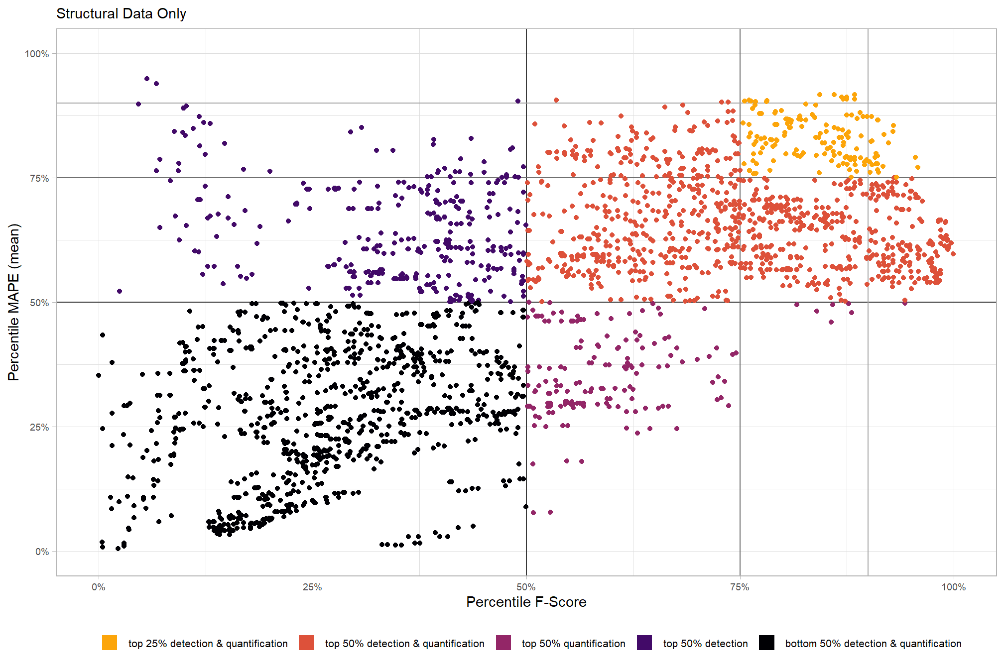
there are a few takeaways from this plot:
- setting the
spectral_weightto “3”, “4”, or “5” improves detection accuracy across CHM resolution levels whereas values of “1” or “2” appear to be similar to including no spectral data at all - including spectral data and setting the
spectral_weightto “5” results in a only a slight change in detection accuracy compared to a value of “4” for the finder resolution CHM data (e.g. 0.2 m or less) but beyond a CHM resolution of ~0.25 m detection accuracy is maximized when setting thespectral_weightto “5”. this makes intuitive sense because as the structural information about slash piles becomes less fine grain (i.e. more coarse), we should put more weight into the spectral data for detecting slash piles
all of this is to say that the impact of spectral_weight varies based on the CHM resolution setting and vice-versa
we can look at the posterior distributions of the expected F-score at different spectral_weight settings by the input CHM resolution
draws_temp %>%
dplyr::filter(
round(chm_res_m,2) == round(chm_res_m,1) # let's just look at every 0.1 m (10 cm)
) %>%
dplyr::mutate(chm_res_m = chm_res_m %>% factor() %>% forcats::fct_relabel(~paste0("CHM resolution: ", .x, recycle0 = T))) %>%
ggplot2::ggplot(mapping = ggplot2::aes(y=value, x=spectral_weight)) +
tidybayes::stat_eye(
mapping = ggplot2::aes(fill = chm_res_m)
, point_interval = median_hdi, .width = .95
, slab_alpha = 0.95
, interval_color = "gray44", linewidth = 1
, point_color = "gray44", point_fill = "gray44", point_size = 1
) +
ggplot2::facet_grid(cols = dplyr::vars(chm_res_m)) +
ggplot2::scale_fill_viridis_d(option = "rocket", begin = 0.9, end = 0.6) +
ggplot2::scale_y_continuous(limits = c(0,NA), labels = scales::percent, breaks = scales::breaks_extended(16)) +
ggplot2::labs(x = "`spectral_weight`", y = "F-score") +
ggplot2::theme_light() +
ggplot2::theme(
legend.position = "none"
, strip.text = ggplot2::element_text(size = 8, color = "black", face = "bold")
)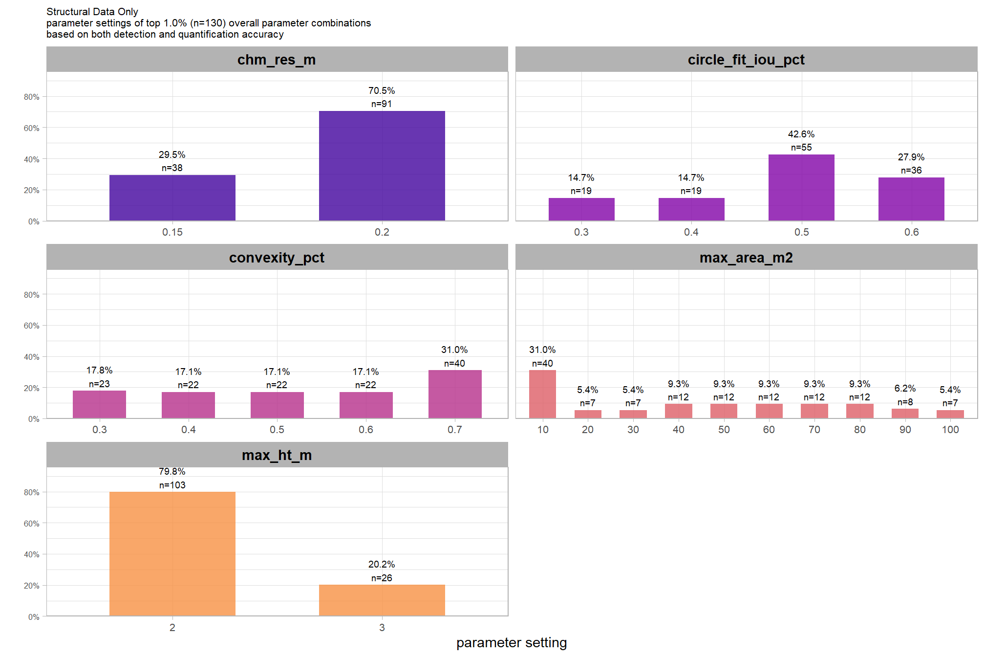
we already saw this same data above in our CHM resolution testing, but we’ll table that again but this time grouping by CHM resolution
draws_temp %>%
dplyr::filter(
round(chm_res_m,2) == round(chm_res_m,1) # let's just look at every 0.1 m (10 cm)
) %>%
dplyr::mutate(chm_res_m = chm_res_m %>% factor() %>% forcats::fct_relabel(~paste0("CHM resolution: ", .x, recycle0 = T))) %>%
dplyr::group_by(chm_res_m, spectral_weight) %>%
dplyr::summarise(
# get median_hdi
median_hdi_est = tidybayes::median_hdci(value)$y
, median_hdi_lower = tidybayes::median_hdci(value)$ymin
, median_hdi_upper = tidybayes::median_hdci(value)$ymax
) %>%
dplyr::ungroup() %>%
dplyr::arrange(chm_res_m,spectral_weight) %>%
# format pcts
dplyr::mutate(dplyr::across(
tidyselect::starts_with("median_hdi_")
, ~ scales::percent(.x, accuracy = 0.1)
)) %>%
kableExtra::kbl(
digits = 2
, caption = "F-score<br>95% HDI of the posterior predictive distribution"
, col.names = c(
"CHM resolution", "spectral_weight"
, c("F-score<br>median", "HDI low", "HDI high")
)
, escape = F
) %>%
kableExtra::kable_styling() %>%
kableExtra::collapse_rows(columns = 1, valign = "top") %>%
kableExtra::scroll_box(height = "8in")| CHM resolution | spectral_weight |
F-score median |
HDI low | HDI high |
|---|---|---|---|---|
| CHM resolution: 0.1 | 0 | 80.9% | 80.2% | 81.5% |
| 1 | 80.9% | 80.2% | 81.6% | |
| 2 | 80.9% | 80.2% | 81.6% | |
| 3 | 81.3% | 80.7% | 82.1% | |
| 4 | 84.9% | 84.3% | 85.5% | |
| 5 | 84.4% | 84.0% | 85.0% | |
| CHM resolution: 0.2 | 0 | 76.0% | 75.3% | 76.6% |
| 1 | 76.0% | 75.4% | 76.7% | |
| 2 | 76.0% | 75.4% | 76.7% | |
| 3 | 76.5% | 76.0% | 77.3% | |
| 4 | 80.4% | 79.9% | 80.9% | |
| 5 | 81.2% | 80.8% | 81.7% | |
| CHM resolution: 0.3 | 0 | 70.3% | 69.7% | 70.9% |
| 1 | 70.3% | 69.7% | 71.0% | |
| 2 | 70.3% | 69.6% | 70.9% | |
| 3 | 70.9% | 70.3% | 71.5% | |
| 4 | 74.9% | 74.4% | 75.6% | |
| 5 | 77.5% | 77.0% | 78.0% | |
| CHM resolution: 0.4 | 0 | 63.9% | 63.1% | 64.7% |
| 1 | 63.9% | 63.1% | 64.7% | |
| 2 | 63.9% | 63.1% | 64.8% | |
| 3 | 64.6% | 63.8% | 65.4% | |
| 4 | 68.5% | 67.8% | 69.3% | |
| 5 | 73.3% | 72.6% | 73.9% | |
| CHM resolution: 0.5 | 0 | 57.0% | 55.8% | 58.1% |
| 1 | 57.0% | 55.9% | 58.1% | |
| 2 | 57.0% | 55.8% | 58.1% | |
| 3 | 57.7% | 56.4% | 58.7% | |
| 4 | 61.4% | 60.2% | 62.4% | |
| 5 | 68.6% | 67.6% | 69.5% |
now we’ll probabilistically test the hypothesis that the inclusion of spectral data improves detection accuracy and quantify by how much. we’ll look at the influence of spectral data based on the CHM resolution
to actually compare the different levels of spectral_weight, we’ll use the MCMC draws to contrast the posterior predictions at different levels of the parameter (see below)
contrast_temp <-
draws_temp %>%
dplyr::filter(
round(chm_res_m,2) == round(chm_res_m,1) # let's just look at every 0.1 m (10 cm)
) %>%
dplyr::group_by(chm_res_m) %>%
tidybayes::compare_levels(
value
, by = spectral_weight
, comparison =
# tidybayes::emmeans_comparison("revpairwise")
"pairwise"
) %>%
# dplyr::glimpse()
dplyr::rename(contrast = spectral_weight) %>%
# group the data before calculating contrast variables %>%
dplyr::group_by(chm_res_m, contrast) %>%
make_contrast_vars() %>%
# relabel the label for the facets
dplyr::mutate(chm_res_m = chm_res_m %>% factor() %>% forcats::fct_relabel(~paste0("CHM resolution: ", .x, recycle0 = T)))
# huh?
# contrast_temp %>% dplyr::glimpse()
# plot it
plt_contrast(
contrast_temp
# , caption_text = form_temp
, y_axis_title = "`spectral_weight` contrast"
, x_axis_title = "difference (F-score)"
, facet = "chm_res_m"
, label_size = 2
, x_expand = c(0.5,0.5)
) +
labs(
subtitle = "posterior predictive distribution of group constrasts with 95% & 50% HDI\nby `chm_res_m`"
)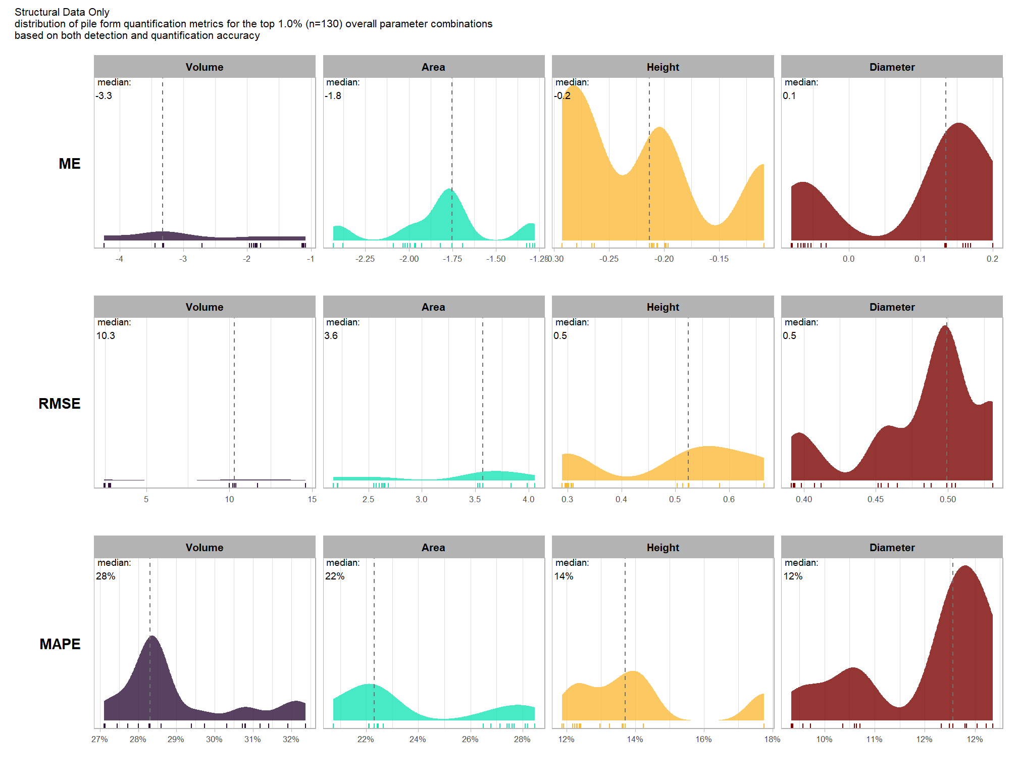
let’s table it
contrast_temp %>%
dplyr::distinct(
chm_res_m, contrast
, median_hdi_est, median_hdi_lower, median_hdi_upper
# , pr_lt_zero
, pr_gt_zero
) %>%
dplyr::arrange(chm_res_m, contrast) %>%
# format pcts
dplyr::mutate(dplyr::across(
tidyselect::starts_with("median_hdi_")
, ~ scales::percent(.x, accuracy = 0.1)
)) %>%
kableExtra::kbl(
digits = 2
, caption = "brms::brm model: 95% HDI of the posterior predictive distribution of group constrasts"
, col.names = c(
"CHM resolution", "spectral_weight"
, "difference (F-score)"
, "HDI low", "HDI high"
# , "Pr(diff<0)"
, "Pr(diff>0)"
)
, escape = F
) %>%
kableExtra::kable_styling() %>%
kableExtra::collapse_rows(columns = 1, valign = "top") %>%
kableExtra::scroll_box(height = "8in")| CHM resolution | spectral_weight | difference (F-score) | HDI low | HDI high | Pr(diff>0) |
|---|---|---|---|---|---|
| CHM resolution: 0.1 | 1 - 0 | 0.0% | -0.8% | 0.9% | 50% |
| 2 - 0 | 0.0% | -0.9% | 0.9% | 49% | |
| 2 - 1 | 0.0% | -0.9% | 0.8% | 51% | |
| 3 - 0 | 0.5% | -0.5% | 1.2% | 84% | |
| 3 - 1 | 0.4% | -0.4% | 1.4% | 83% | |
| 3 - 2 | 0.4% | -0.4% | 1.4% | 84% | |
| 4 - 0 | 4.0% | 3.2% | 4.8% | 100% | |
| 4 - 1 | 4.0% | 3.2% | 4.7% | 100% | |
| 4 - 2 | 4.0% | 3.3% | 4.8% | 100% | |
| 4 - 3 | 3.6% | 2.8% | 4.3% | 100% | |
| 5 - 0 | 3.6% | 2.8% | 4.4% | 100% | |
| 5 - 1 | 3.6% | 2.8% | 4.3% | 100% | |
| 5 - 2 | 3.5% | 2.9% | 4.3% | 100% | |
| 5 - 3 | 3.1% | 2.3% | 3.8% | 100% | |
| 5 - 4 | -0.5% | -1.2% | 0.1% | 9% | |
| CHM resolution: 0.2 | 1 - 0 | 0.0% | -0.7% | 0.8% | 52% |
| 2 - 0 | 0.0% | -0.8% | 0.7% | 51% | |
| 2 - 1 | 0.0% | -0.8% | 0.7% | 50% | |
| 3 - 0 | 0.5% | -0.3% | 1.2% | 91% | |
| 3 - 1 | 0.5% | -0.2% | 1.3% | 90% | |
| 3 - 2 | 0.5% | -0.2% | 1.3% | 92% | |
| 4 - 0 | 4.4% | 3.7% | 5.0% | 100% | |
| 4 - 1 | 4.4% | 3.8% | 5.1% | 100% | |
| 4 - 2 | 4.4% | 3.8% | 5.1% | 100% | |
| 4 - 3 | 3.9% | 3.3% | 4.6% | 100% | |
| 5 - 0 | 5.2% | 4.6% | 5.9% | 100% | |
| 5 - 1 | 5.2% | 4.5% | 5.8% | 100% | |
| 5 - 2 | 5.2% | 4.6% | 5.9% | 100% | |
| 5 - 3 | 4.7% | 4.1% | 5.3% | 100% | |
| 5 - 4 | 0.8% | 0.2% | 1.4% | 100% | |
| CHM resolution: 0.3 | 1 - 0 | 0.0% | -0.7% | 0.8% | 52% |
| 2 - 0 | 0.0% | -0.7% | 0.7% | 50% | |
| 2 - 1 | 0.0% | -0.8% | 0.7% | 48% | |
| 3 - 0 | 0.6% | -0.2% | 1.3% | 94% | |
| 3 - 1 | 0.6% | -0.1% | 1.3% | 94% | |
| 3 - 2 | 0.6% | -0.2% | 1.2% | 95% | |
| 4 - 0 | 4.6% | 4.0% | 5.3% | 100% | |
| 4 - 1 | 4.6% | 4.0% | 5.3% | 100% | |
| 4 - 2 | 4.6% | 4.0% | 5.4% | 100% | |
| 4 - 3 | 4.0% | 3.4% | 4.7% | 100% | |
| 5 - 0 | 7.2% | 6.6% | 7.8% | 100% | |
| 5 - 1 | 7.2% | 6.6% | 7.8% | 100% | |
| 5 - 2 | 7.2% | 6.6% | 7.8% | 100% | |
| 5 - 3 | 6.6% | 6.0% | 7.2% | 100% | |
| 5 - 4 | 2.6% | 1.9% | 3.1% | 100% | |
| CHM resolution: 0.4 | 1 - 0 | 0.0% | -0.9% | 1.0% | 52% |
| 2 - 0 | 0.0% | -1.0% | 0.9% | 52% | |
| 2 - 1 | 0.0% | -1.0% | 1.0% | 48% | |
| 3 - 0 | 0.6% | -0.3% | 1.6% | 89% | |
| 3 - 1 | 0.6% | -0.3% | 1.6% | 89% | |
| 3 - 2 | 0.6% | -0.4% | 1.7% | 89% | |
| 4 - 0 | 4.6% | 3.6% | 5.5% | 100% | |
| 4 - 1 | 4.6% | 3.8% | 5.6% | 100% | |
| 4 - 2 | 4.6% | 3.7% | 5.6% | 100% | |
| 4 - 3 | 4.0% | 3.0% | 4.9% | 100% | |
| 5 - 0 | 9.4% | 8.5% | 10.3% | 100% | |
| 5 - 1 | 9.3% | 8.5% | 10.1% | 100% | |
| 5 - 2 | 9.3% | 8.4% | 10.2% | 100% | |
| 5 - 3 | 8.7% | 7.8% | 9.6% | 100% | |
| 5 - 4 | 4.7% | 3.9% | 5.5% | 100% | |
| CHM resolution: 0.5 | 1 - 0 | 0.0% | -1.4% | 1.5% | 53% |
| 2 - 0 | 0.0% | -1.5% | 1.4% | 51% | |
| 2 - 1 | 0.0% | -1.3% | 1.5% | 50% | |
| 3 - 0 | 0.7% | -0.8% | 2.1% | 81% | |
| 3 - 1 | 0.6% | -0.8% | 2.1% | 80% | |
| 3 - 2 | 0.6% | -0.7% | 2.3% | 80% | |
| 4 - 0 | 4.4% | 2.8% | 5.8% | 100% | |
| 4 - 1 | 4.4% | 3.0% | 5.7% | 100% | |
| 4 - 2 | 4.3% | 2.9% | 5.7% | 100% | |
| 4 - 3 | 3.7% | 2.2% | 5.0% | 100% | |
| 5 - 0 | 11.6% | 10.3% | 12.9% | 100% | |
| 5 - 1 | 11.6% | 10.5% | 13.0% | 100% | |
| 5 - 2 | 11.6% | 10.3% | 12.9% | 100% | |
| 5 - 3 | 10.9% | 9.7% | 12.4% | 100% | |
| 5 - 4 | 7.2% | 6.0% | 8.4% | 100% |
We’ve previously observed that setting the spectral_weight to “1” or “2” appears to have minimal impact on detection accuracy, with improvements only becoming apparent at levels of “3,” “4,” or “5.” These contrasts allow us to evaluate those hypotheses probabilistically. At a 0.2m CHM resolution, for example, there is no evidence that including spectral data but setting spectral_weight to “1” is better or worse than not including it at all (spectral_weight = “0”). Although setting spectral_weight to “3” provides a highly certain improvement in detection accuracy (~90% probability) compared to not using any spectral data, the improvement is small, at less than one percentage point. The model indicates with high certainty (>99% probability) that the optimal setting for 0.2m CHM data is spectral_weight = “5,” which improves F-score by 6 percentage points compared to not including spectral data at all.
For coarser CHM data (e.g., >0.3m), we can be highly confident (>99% probability) that spectral_weight set to “5” is the optimal setting for detection accuracy. At this setting, F-score is increased by 10 percentage points for 0.4m resolution rasters and by 12 percentage points for 0.5m resolution rasters when compared to not including spectral data at all.
9.2 Bayesian GLM - Diameter MAPE
9.2.1 Model selection
we’re going to use a sub-sample of the data to perform model testing. our objective is to construct the model such that it faithfully represents the data.
we reviewed the main effect parameter trends against MAPE here and used these to guide our model design. we’ll follow Kurz 2025 and compare our models with the LOO information criterion
Like other information criteria, the LOO values aren’t of interest in and of themselves. However, the values of one model’s LOO relative to that of another is of great interest. We generally prefer models with lower estimates.
# subsample data
set.seed(222)
ms_df_temp <- param_combos_spectral_ranked %>% dplyr::slice_sample(prop = 0.11)
# mcmc setup
iter_temp <- 2444
warmup_temp <- 1222
chains_temp <- 4
####################################################################
# base model with form selected based on main effect trends
####################################################################
diam_mape_mod1_temp <- brms::brm(
formula = pct_diff_diameter_m_mape ~
0 + # no intercept to allow all values of spectral_weight to be shown instead of set as the baseline
max_ht_m + max_area_m2 + convexity_pct + circle_fit_iou_pct +
chm_res_m +
spectral_weight + chm_res_m:spectral_weight
, data = ms_df_temp
, family = Gamma(link = "log")
# mcmc
, iter = iter_temp, warmup = warmup_temp
, chains = chains_temp
# , control = list(adapt_delta = 0.999, max_treedepth = 13)
, cores = lasR::half_cores()
, file = paste0("../data/", "diam_mape_mod1_temp")
)
diam_mape_mod1_temp <- brms::add_criterion(diam_mape_mod1_temp, criterion = "loo")
####################################################################
# allows slope and curvature of circle_fit_iou_pct to vary by chm_res_m and vice-versa
####################################################################
diam_mape_mod2_temp <- brms::brm(
formula = pct_diff_diameter_m_mape ~
0 + # no intercept to allow all values of spectral_weight to be shown instead of set as the baseline
max_ht_m + max_area_m2 + convexity_pct +
circle_fit_iou_pct + I(circle_fit_iou_pct^2) + # changed from base model
chm_res_m +
spectral_weight + chm_res_m:spectral_weight
, data = ms_df_temp
, family = Gamma(link = "log")
# mcmc
, iter = iter_temp, warmup = warmup_temp
, chains = chains_temp
# , control = list(adapt_delta = 0.999, max_treedepth = 13)
, cores = lasR::half_cores()
, file = paste0("../data/", "diam_mape_mod2_temp")
)
diam_mape_mod2_temp <- brms::add_criterion(diam_mape_mod2_temp, criterion = "loo")
####################################################################
# allows slope and curvature of circle_fit_iou_pct to vary by convexity_pct and vice-versa
####################################################################
diam_mape_mod3_temp <- brms::brm(
formula = pct_diff_diameter_m_mape ~
0 + # no intercept to allow all values of spectral_weight to be shown instead of set as the baseline
max_ht_m + max_area_m2 +
convexity_pct + I(convexity_pct^2) + # changed from base model
circle_fit_iou_pct + I(circle_fit_iou_pct^2) + # changed from base model
convexity_pct:circle_fit_iou_pct + # changed from base model
chm_res_m +
spectral_weight + chm_res_m:spectral_weight
, data = ms_df_temp
, family = Gamma(link = "log")
# mcmc
, iter = iter_temp, warmup = warmup_temp
, chains = chains_temp
# , control = list(adapt_delta = 0.999, max_treedepth = 13)
, cores = lasR::half_cores()
, file = paste0("../data/", "diam_mape_mod3_temp")
)
diam_mape_mod3_temp <- brms::add_criterion(diam_mape_mod3_temp, criterion = "loo")
####################################################################
# a three-way interaction of circle_fit_iou_pct, convexity_pct and chm_res_m
####################################################################
diam_mape_mod4_temp <- brms::brm(
formula = pct_diff_diameter_m_mape ~
0 + # no intercept to allow all values of spectral_weight to be shown instead of set as the baseline
max_ht_m + max_area_m2 +
convexity_pct + I(convexity_pct^2) + # changed from base model
circle_fit_iou_pct + I(circle_fit_iou_pct^2) + # changed from base model
convexity_pct:circle_fit_iou_pct + # changed from base model
chm_res_m + I(chm_res_m^2) + # changed from base model
spectral_weight + chm_res_m:spectral_weight
, data = ms_df_temp
, family = Gamma(link = "log")
# mcmc
, iter = iter_temp, warmup = warmup_temp
, chains = chains_temp
# , control = list(adapt_delta = 0.999, max_treedepth = 13)
, cores = lasR::half_cores()
, file = paste0("../data/", "diam_mape_mod4_temp")
)
diam_mape_mod4_temp <- brms::add_criterion(diam_mape_mod4_temp, criterion = "loo")
####################################################################
# a three-way interaction of circle_fit_iou_pct, convexity_pct and chm_res_m
####################################################################
diam_mape_mod5_temp <- brms::brm(
formula = pct_diff_diameter_m_mape ~
0 + # no intercept to allow all values of spectral_weight to be shown instead of set as the baseline
max_ht_m + max_area_m2 +
convexity_pct + I(convexity_pct^2) + # changed from base model
circle_fit_iou_pct + I(circle_fit_iou_pct^2) + # changed from base model
convexity_pct:circle_fit_iou_pct + # changed from base model
convexity_pct:chm_res_m + # changed from base model
circle_fit_iou_pct:chm_res_m + # changed from base model
convexity_pct:circle_fit_iou_pct:chm_res_m + # changed from base model
chm_res_m +
spectral_weight + chm_res_m:spectral_weight
, data = ms_df_temp
, family = Gamma(link = "log")
# mcmc
, iter = iter_temp, warmup = warmup_temp
, chains = chains_temp
# , control = list(adapt_delta = 0.999, max_treedepth = 13)
, cores = lasR::half_cores()
, file = paste0("../data/", "diam_mape_mod5_temp")
)
diam_mape_mod5_temp <- brms::add_criterion(diam_mape_mod5_temp, criterion = "loo")
####################################################################
# a three-way interaction of circle_fit_iou_pct, convexity_pct and chm_res_m
####################################################################
diam_mape_mod6_temp <- brms::brm(
formula = pct_diff_diameter_m_mape ~
0 + # no intercept to allow all values of spectral_weight to be shown instead of set as the baseline
max_ht_m + max_area_m2 +
convexity_pct + I(convexity_pct^2) + # changed from base model
circle_fit_iou_pct + I(circle_fit_iou_pct^2) + # changed from base model
convexity_pct:circle_fit_iou_pct + # changed from base model
convexity_pct:chm_res_m + # changed from base model
circle_fit_iou_pct:chm_res_m + # changed from base model
convexity_pct:circle_fit_iou_pct:chm_res_m + # changed from base model
chm_res_m + I(chm_res_m^2) + # changed from base model
spectral_weight + chm_res_m:spectral_weight
, data = ms_df_temp
, family = Gamma(link = "log")
# mcmc
, iter = iter_temp, warmup = warmup_temp
, chains = chains_temp
# , control = list(adapt_delta = 0.999, max_treedepth = 13)
, cores = lasR::half_cores()
, file = paste0("../data/", "diam_mape_mod6_temp")
)
diam_mape_mod6_temp <- brms::add_criterion(diam_mape_mod6_temp, criterion = "loo")compare our models with the LOO information criterion. with the brms::loo_compare() function, we can compute a formal difference score between models with the output rank ordering the models such that the best fitting model appears on top. all models also receive a difference score relative to the best model and a standard error of the difference score
brms::loo_compare(
diam_mape_mod1_temp, diam_mape_mod2_temp, diam_mape_mod3_temp
, diam_mape_mod4_temp, diam_mape_mod5_temp, diam_mape_mod6_temp
) %>%
kableExtra::kbl(caption = "Diameter MAPE model selection with LOO information criterion") %>%
kableExtra::kable_styling()| elpd_diff | se_diff | elpd_loo | se_elpd_loo | p_loo | se_p_loo | looic | se_looic | |
|---|---|---|---|---|---|---|---|---|
| diam_mape_mod6_temp | 0.00000 | 0.000000 | 4858.224 | 230.2337 | 50.45998 | 8.675364 | -9716.447 | 460.4674 |
| diam_mape_mod4_temp | -27.48832 | 9.248765 | 4830.735 | 230.5794 | 45.42794 | 7.940583 | -9661.471 | 461.1589 |
| diam_mape_mod5_temp | -209.19202 | 23.057174 | 4649.032 | 209.4472 | 43.45478 | 7.092683 | -9298.063 | 418.8943 |
| diam_mape_mod3_temp | -225.57831 | 23.411588 | 4632.645 | 210.1472 | 39.40540 | 6.586324 | -9265.291 | 420.2943 |
| diam_mape_mod2_temp | -241.68897 | 25.707239 | 4616.535 | 208.9627 | 39.61183 | 6.834882 | -9233.070 | 417.9254 |
| diam_mape_mod1_temp | -255.46016 | 25.441375 | 4602.764 | 209.4960 | 37.39897 | 6.526955 | -9205.527 | 418.9920 |
we can also look at the AIC-type model weights
brms::model_weights(
diam_mape_mod1_temp, diam_mape_mod2_temp, diam_mape_mod3_temp
, diam_mape_mod4_temp, diam_mape_mod5_temp, diam_mape_mod6_temp
) %>%
round(digits = 4)we can also quickly look at the Bayeisan \(R^2\) returned from the brms::bayes_R2() function
dplyr::bind_rows(
brms::bayes_R2(diam_mape_mod1_temp,summary=F) %>% dplyr::as_tibble() %>% dplyr::mutate(mod = "diam_mape_mod1_temp")
, brms::bayes_R2(diam_mape_mod2_temp,summary=F) %>% dplyr::as_tibble() %>% dplyr::mutate(mod = "diam_mape_mod2_temp")
, brms::bayes_R2(diam_mape_mod3_temp,summary=F) %>% dplyr::as_tibble() %>% dplyr::mutate(mod = "diam_mape_mod3_temp")
, brms::bayes_R2(diam_mape_mod4_temp,summary=F) %>% dplyr::as_tibble() %>% dplyr::mutate(mod = "diam_mape_mod4_temp")
, brms::bayes_R2(diam_mape_mod5_temp,summary=F) %>% dplyr::as_tibble() %>% dplyr::mutate(mod = "diam_mape_mod5_temp")
, brms::bayes_R2(diam_mape_mod6_temp,summary=F) %>% dplyr::as_tibble() %>% dplyr::mutate(mod = "diam_mape_mod6_temp")
) %>%
dplyr::mutate(mod = factor(mod)) %>%
ggplot2::ggplot(mapping=ggplot2::aes(y=R2, x = mod)) +
tidybayes::stat_eye(
point_interval = median_hdi, .width = .95
, slab_alpha = 0.95
) +
# ggplot2::facet_grid(cols = dplyr::vars(spectral_weight)) +
# ggplot2::scale_fill_manual(values = pal_chm_res_m) +
ggplot2::labs(x = "", y = "Bayesian R-squared") +
ggplot2::theme_light()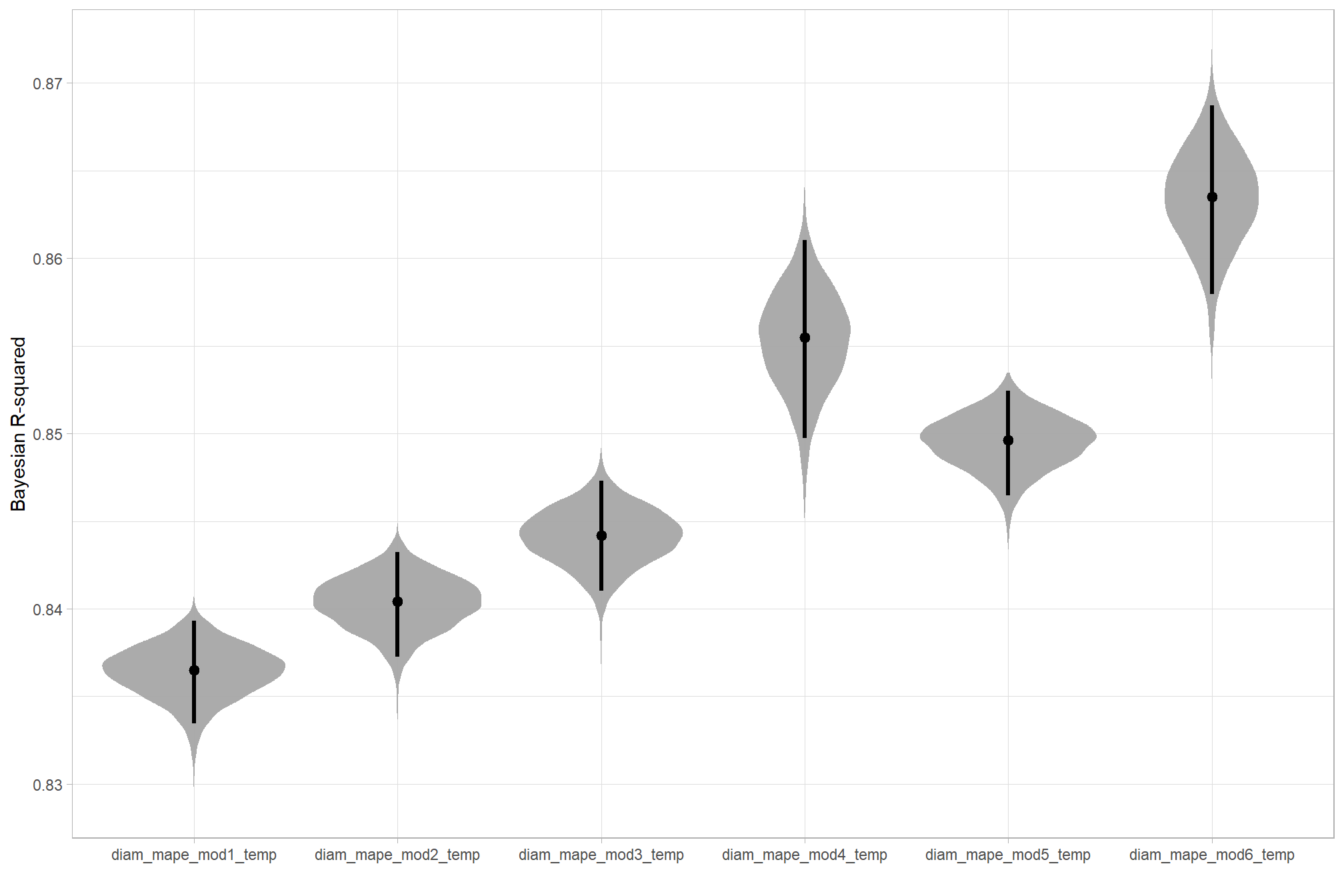
the more complex models were selected as the best. because the selected model includes quadratic terms and multiple interactions parameter interpretation will be a challenge, so we will have to rely on plotting the modeled relationships rather than trying to interpret the coefficients.
9.2.2 Modeling
the selected MAPE model predicts diameter error using the four structural parameters (max_ht_m, max_area_m2, convexity_pct, circle_fit_iou_pct) and data properties representing the CHM resolution (chm_res_m) and the use of spectral data (spectral_weight). The model includes quadratic terms for both chm_res_m and circle_fit_iou_pct to allow for non-linear relationships between these parameters and MAPE.
To account for how different parameters influence each other, the model includes several interaction terms. The circle_fit_iou_pct:chm_res_m and the circle_fit_iou_pct:convexity_pct interactions were included to explore how the effect of the geometric filtering parameters varies with CHM resolution and with each other. In addition, the model includes spectral_weight as a main effect and in an interaction with chm_res_m. This means that the predicted MAPE can vary by the spectral_weight setting even when all other variables are zero (i.e. the intercept), effectively giving each level of spectral_weight its own unique intercept. Finally, the chm_res_m:spectral_weight interaction allows the effect of CHM resolution (i.e. its slope) on MAPE to vary across each spectral_weight setting.
the fully factored Bayesian statistical model that details the likelihood, linear model, and priors used is:
\[\begin{align*} \text{MAPE}_i \sim & \operatorname{Gamma}(\mu_i, \text{shape}) \\ \log(\mu_i) = & (\beta_1 \cdot \text{max_ht_m}_i) + (\beta_2 \cdot \text{max_area_m2}_i) \\ & + (\beta_3 \cdot \text{convexity_pct}_i) + (\beta_4 \cdot (\text{convexity_pct}_i)^2) \\ & + (\beta_5 \cdot \text{circle_fit_iou_pct}_i) + (\beta_6 \cdot (\text{circle_fit_iou_pct}_i)^2) \\ & + (\beta_7 \cdot \text{chm_res_m}_i) + (\beta_8 \cdot (\text{chm_res_m}_i)^2) \\ & + \sum_{j=0}^{5} \left( \beta_{9, j} \cdot \mathbf{I}(\text{spectral_weight}_i = j) \right) \\ & + (\beta_{10} \cdot \text{convexity_pct}_i \cdot \text{circle_fit_iou_pct}_i) \\ & + (\beta_{11} \cdot \text{convexity_pct}_i \cdot \text{chm_res_m}_i) \\ & + (\beta_{12} \cdot \text{circle_fit_iou_pct}_i \cdot \text{chm_res_m}_i) \\ & + \sum_{j=0}^{5} \left( \beta_{13, j} \cdot \text{chm_res_m}_i \cdot \mathbf{I}(\text{spectral_weight}_i = j) \right) \\ & + (\beta_{14} \cdot \text{convexity_pct}_i \cdot \text{circle_fit_iou_pct}_i \cdot \text{chm_res_m}_i) \\ \beta_k \sim & \operatorname{Student-t}(3, 0, 10) \quad \text{for } k = 1, \dots, 14 \\ \text{shape} \sim & \operatorname{Gamma}(0.01, 0.01) \end{align*}\]
where, \(i\) represents a single observation in the dataset which corresponds to a specific combination of the six parameters (, max_ht_m, max_area_m2, convexity_pct, circle_fit_iou_pct, chm_res_m, and spectral_weight) and its resulting MAPE. Where k is used to index the different beta coefficients, which correspond to the intercept and the effects of each of the independent variables and their interactions and j denotes the specific level of the nominal (i.e. categorical) predictor spectral_weight
we reviewed the main effect parameter trends against MAPE here and used these to guide our model design
The table below details the terms used in our Bayesian GLM model defined in the brms::brm() call:
| Term in Formula | Type of Effect | Description of Relationship Tested |
|---|---|---|
0 + |
Zero Intercept | Specifies that the model is fit without a global intercept. The effect of each factor level and the value of continuous variables at zero is estimated directly. |
max_ht_m |
Main Effect (Linear) | Tests the direct linear influence of the maximum pile height threshold on MAPE. |
max_area_m2 |
Main Effect (Linear) | Tests the direct linear influence of the maximum pile area threshold on MAPE. |
chm_res_m |
Main Effect (Linear) | Tests the direct linear influence of the input CHM resolution on MAPE. |
I(chm_res_m^2) |
Nonlinear (Quadratic) | Models a curved relationship with CHM resolution, allowing MAPE to potentially decrease then increase (or vice versa) as resolution changes. |
spectral_weight |
Main Effect (Factor) | The model estimates a coefficient for each of the six spectral weight levels (0 through 5), representing the estimated mean MAPE for that specific level when all continuous variables are zero. |
circle_fit_iou_pct |
Main Effect (Linear) | Tests the direct linear influence of the pile’s circular conformity threshold on MAPE. |
convexity_pct |
Main Effect (Linear) | Tests the direct linear influence of the pile’s boundary smoothness (convexity) threshold on MAPE. |
I(circle_fit_iou_pct^2) |
Nonlinear (Quadratic) | Models a curved relationship where MAPE may peak or bottom out at an intermediate threshold for pile circularity. |
I(convexity_pct^2) |
Nonlinear (Quadratic) | Models a curved relationship where MAPE may peak or bottom out at an intermediate threshold for pile boundary smoothness. |
convexity_pct:circle_fit_iou_pct |
Two-Way Interaction | Captures how the optimal balance between pile circular conformity and boundary smoothness changes for MAPE. |
chm_res_m:spectral_weight |
Two-Way Interaction (Factor) | Captures how the effect of CHM resolution’s slope on MAPE changes across each of the six spectral weighting levels. |
convexity_pct:chm_res_m |
Two-Way Interaction | Captures how the sensitivity to the pile boundary smoothness threshold changes with the input data resolution. |
circle_fit_iou_pct:chm_res_m |
Two-Way Interaction | Captures how the importance of the pile’s circular conformity threshold changes as the input data resolution changes. |
convexity_pct:circle_fit_iou_pct:chm_res_m |
Three-Way Interaction | Shows how the combined effects of the convexity and circularity thresholds change simultaneously across different input CHM resolutions. |
brms_diam_mape_mod <- brms::brm(
formula = pct_diff_diameter_m_mape ~
0 + # no intercept to allow all values of spectral_weight to be shown instead of set as the baseline
max_ht_m + max_area_m2 +
convexity_pct + I(convexity_pct^2) + # changed from base model
circle_fit_iou_pct + I(circle_fit_iou_pct^2) + # changed from base model
convexity_pct:circle_fit_iou_pct + # changed from base model
convexity_pct:chm_res_m + # changed from base model
circle_fit_iou_pct:chm_res_m + # changed from base model
convexity_pct:circle_fit_iou_pct:chm_res_m + # changed from base model
chm_res_m + I(chm_res_m^2) + # changed from base model
spectral_weight + chm_res_m:spectral_weight
, data = param_combos_spectral_ranked # %>% dplyr::slice_sample(prop = 0.33)
, family = Gamma(link = "log")
# mcmc
, iter = 14000, warmup = 7000
, chains = 4
# , control = list(adapt_delta = 0.999, max_treedepth = 13)
, cores = lasR::half_cores()
, file = paste0("../data/", "brms_diam_mape_mod")
)
# brms::make_stancode(brms_diam_mape_mod)
# brms::prior_summary(brms_diam_mape_mod)
# print(brms_diam_mape_mod)
# brms::neff_ratio(brms_diam_mape_mod)
# brms::rhat(brms_diam_mape_mod)
# brms::nuts_params(brms_diam_mape_mod)The brms::brm model summary
brms_diam_mape_mod %>%
brms::posterior_summary() %>%
as.data.frame() %>%
tibble::rownames_to_column(var = "parameter") %>%
dplyr::rename_with(tolower) %>%
dplyr::filter(
stringr::str_starts(parameter, "b_")
| parameter == "phi"
) %>%
kableExtra::kbl(digits = 3, caption = "Bayesian model for Diameter MAPE") %>%
kableExtra::kable_styling()| parameter | estimate | est.error | q2.5 | q97.5 |
|---|---|---|---|---|
| b_max_ht_m | 0.008 | 0.001 | 0.005 | 0.010 |
| b_max_area_m2 | 0.001 | 0.000 | 0.001 | 0.001 |
| b_convexity_pct | 0.182 | 0.027 | 0.130 | 0.234 |
| b_Iconvexity_pctE2 | -0.305 | 0.017 | -0.339 | -0.271 |
| b_circle_fit_iou_pct | 0.430 | 0.031 | 0.370 | 0.492 |
| b_Icircle_fit_iou_pctE2 | -0.481 | 0.023 | -0.526 | -0.436 |
| b_chm_res_m | 6.855 | 0.063 | 6.733 | 6.979 |
| b_Ichm_res_mE2 | -5.378 | 0.080 | -5.534 | -5.221 |
| b_spectral_weight0 | -2.967 | 0.016 | -2.999 | -2.936 |
| b_spectral_weight1 | -2.967 | 0.016 | -2.998 | -2.936 |
| b_spectral_weight2 | -2.967 | 0.016 | -2.999 | -2.936 |
| b_spectral_weight3 | -2.967 | 0.016 | -2.999 | -2.936 |
| b_spectral_weight4 | -2.967 | 0.016 | -2.998 | -2.936 |
| b_spectral_weight5 | -2.902 | 0.016 | -2.933 | -2.871 |
| b_convexity_pct:circle_fit_iou_pct | -0.245 | 0.045 | -0.334 | -0.159 |
| b_convexity_pct:chm_res_m | -0.135 | 0.064 | -0.261 | -0.011 |
| b_circle_fit_iou_pct:chm_res_m | -0.924 | 0.072 | -1.065 | -0.783 |
| b_chm_res_m:spectral_weight1 | 0.000 | 0.033 | -0.064 | 0.065 |
| b_chm_res_m:spectral_weight2 | 0.000 | 0.033 | -0.064 | 0.064 |
| b_chm_res_m:spectral_weight3 | 0.000 | 0.033 | -0.064 | 0.064 |
| b_chm_res_m:spectral_weight4 | 0.000 | 0.033 | -0.064 | 0.065 |
| b_chm_res_m:spectral_weight5 | -0.114 | 0.033 | -0.178 | -0.049 |
| b_convexity_pct:circle_fit_iou_pct:chm_res_m | 1.372 | 0.131 | 1.117 | 1.631 |
note the quadratic coefficients ending in E2, Kruschke (2015) provides some insight on how to interpret:
A quadratic has the form \(y = \beta_{0} + \beta_{1}x + \beta_{2}x^{2}\). When \(\beta_{2}\) is zero, the form reduces to a line. Therefore, this extended model can produce any fit that the linear model can. When \(\beta_{2}\) is positive, a plot of the curve is a parabola that opens upward. When \(\beta_{2}\) is negative, the curve is a parabola that opens downward. We have no reason to think that the curvature in the family-income data is exactly a parabola, but the quadratic trend might describe the data much better than a line alone. (p. 496)
9.2.3 Posterior Predictive Checks
Markov chain Monte Carlo (MCMC) simulations were conducted using the brms package (Bürkner 2017) to estimate posterior predictive distributions of the parameters of interest. We ran 4 chains of 10,000 iterations with the first 5,000 discarded as burn-in. Trace-plots were utilized to visually assess model convergence.
check the trace plots for problems with convergence of the Markov chains
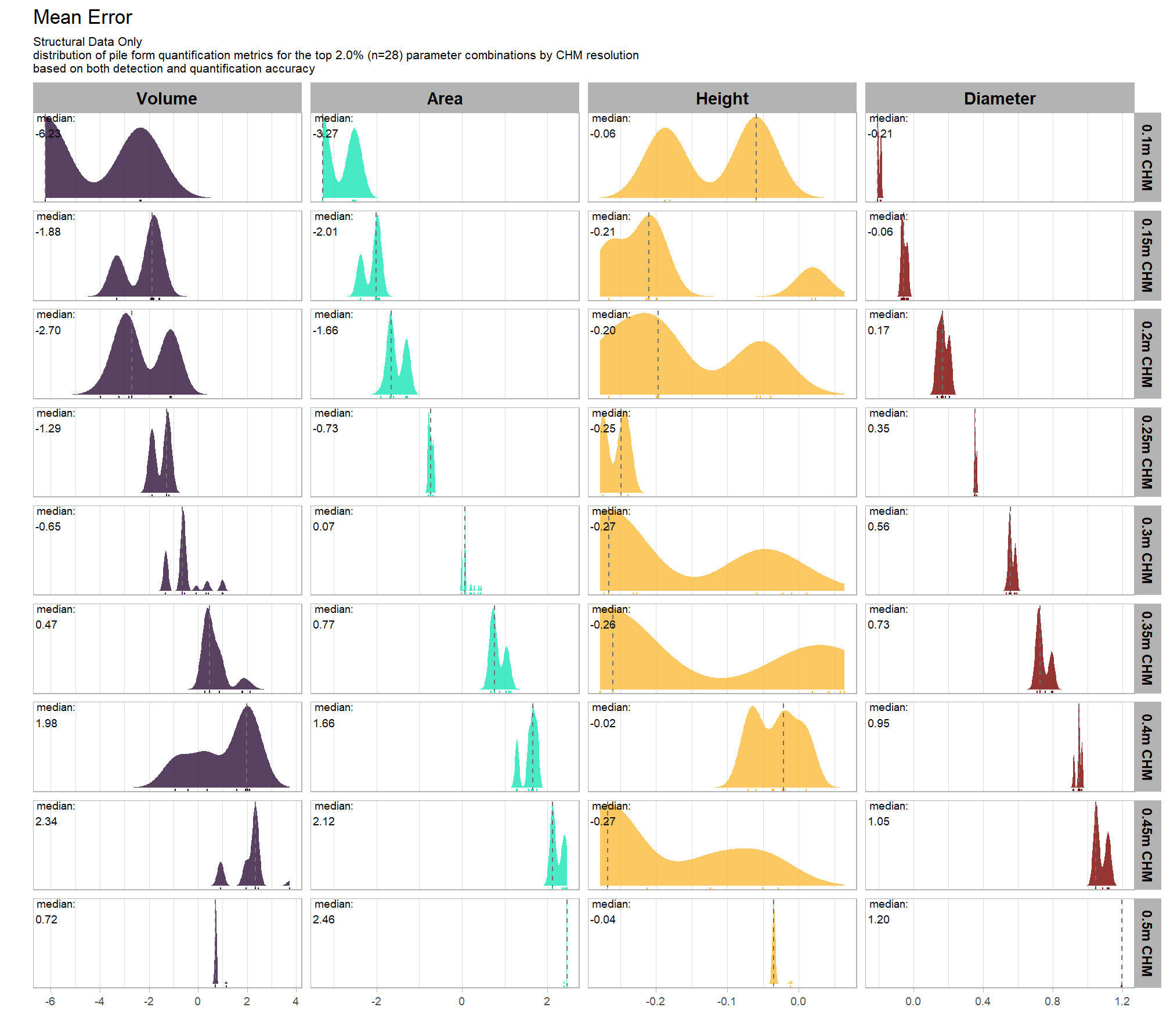
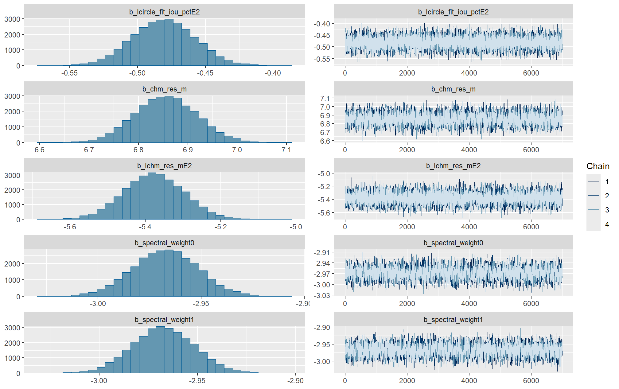
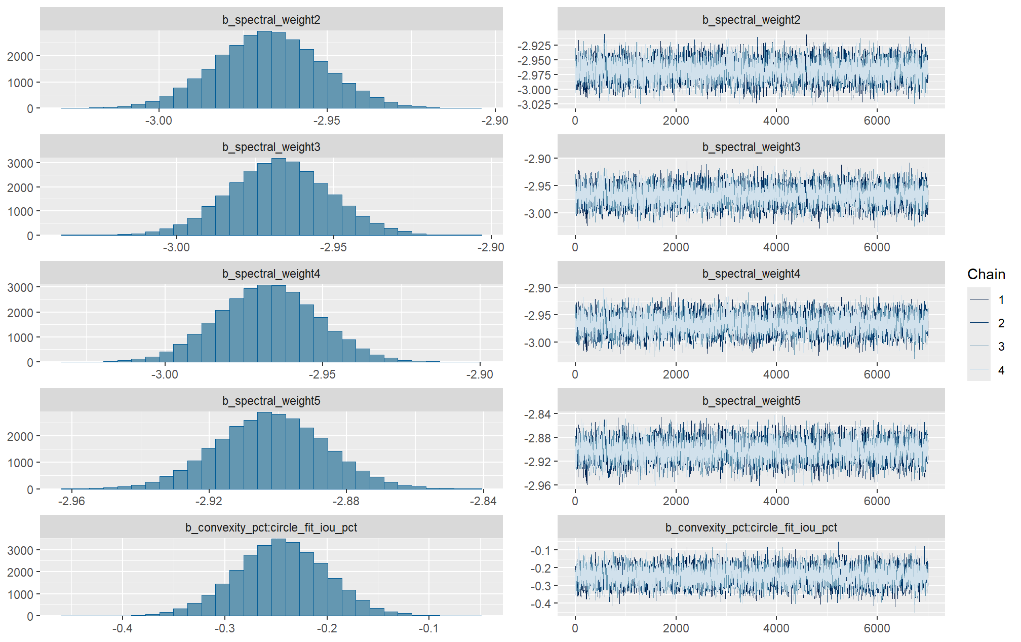
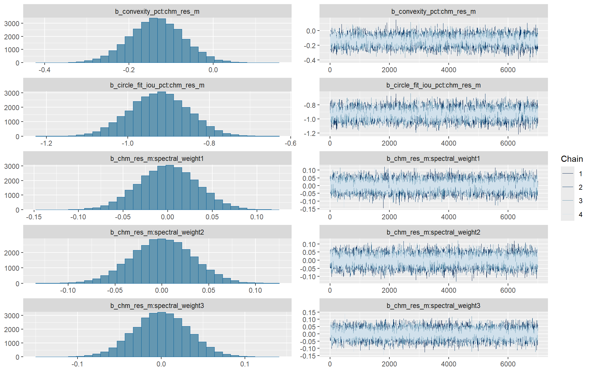
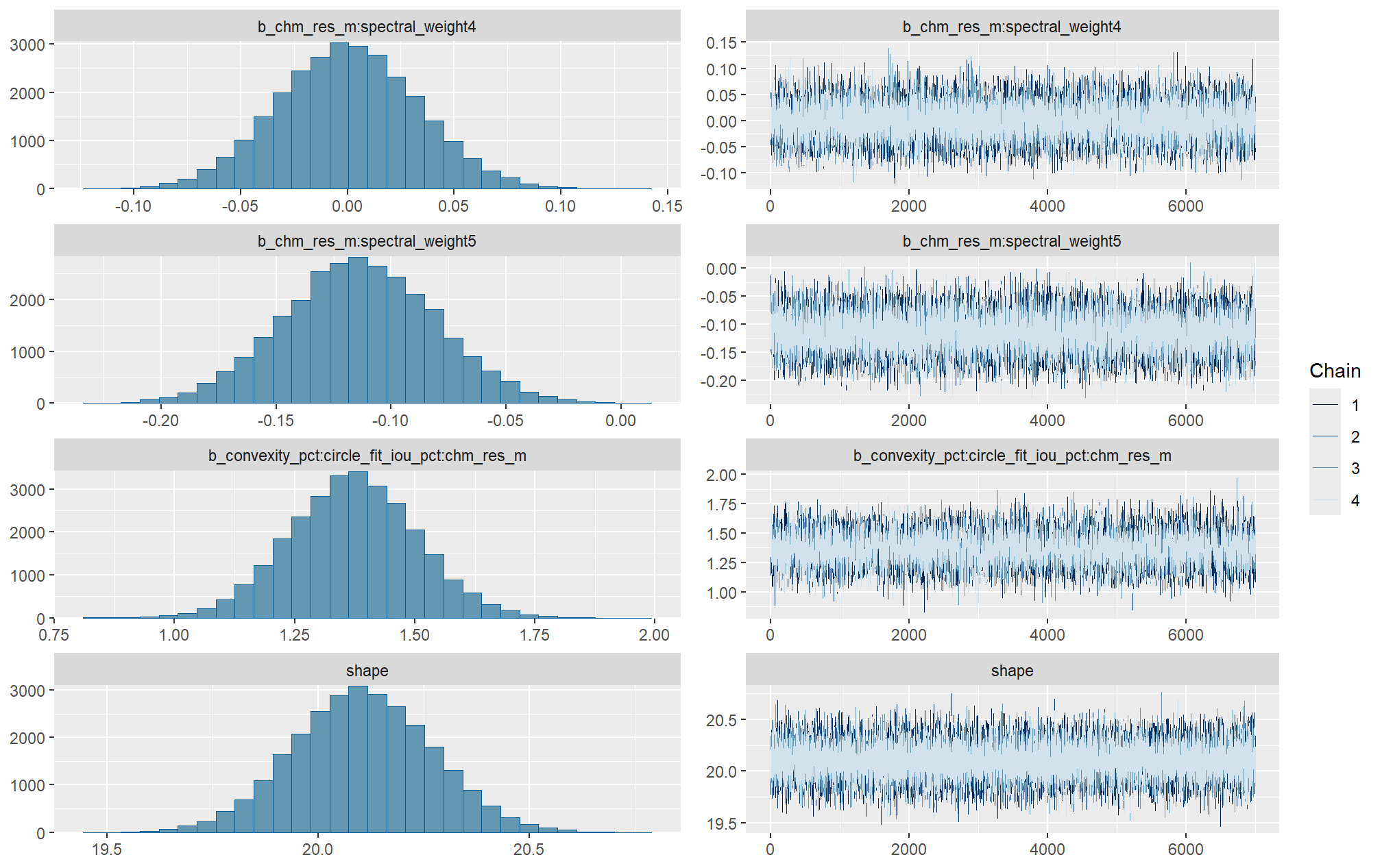
Sufficient convergence was checked with \(\hat{R}\) values near 1 (Brooks & Gelman, 1998).
in the plot below, \(\hat{R}\) values are colored using different shades (lighter is better). The chosen thresholds are somewhat arbitrary, but can be useful guidelines in practice (Gabry and Mahr 2025):
- light: below 1.05 (good)
- mid: between 1.05 and 1.1 (ok)
- dark: above 1.1 (too high)
check our \(\hat{R}\) values
brms::mcmc_plot(brms_diam_mape_mod, type = "rhat_hist") +
ggplot2::scale_x_continuous(breaks = scales::breaks_extended(n = 6)) +
ggplot2::theme_light() +
ggplot2::theme(
legend.position = "top", legend.direction = "horizontal"
)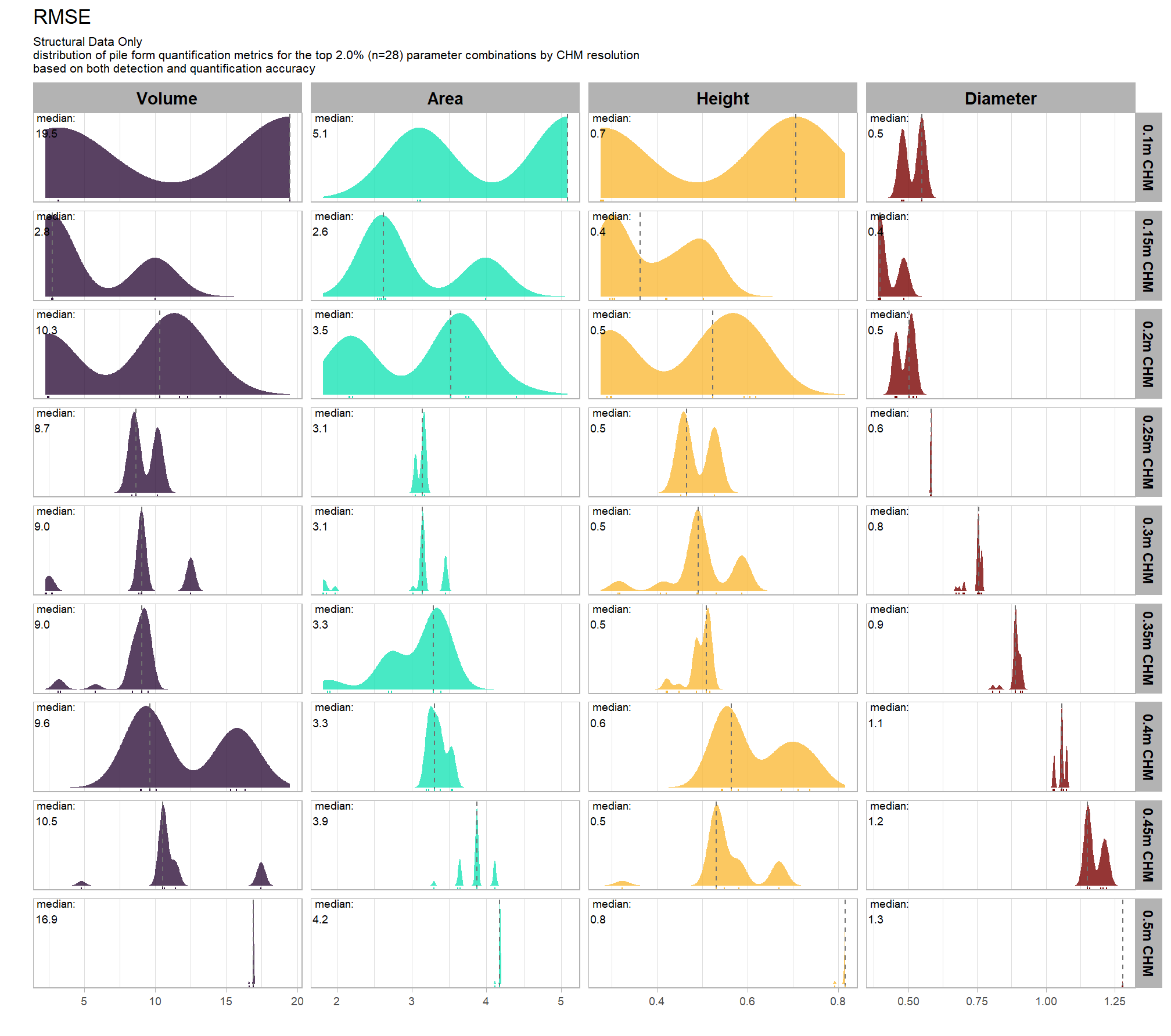
The effective length of an MCMC chain is indicated by the effective sample size (ESS), which refers to the sample size of the MCMC chain not to the sample size of the data where acceptable values allow “for reasonably accurate and stable estimates of the limits of the 95% HDI…If accuracy of the HDI limits is not crucial for your application, then a smaller ESS may be sufficient” (Kruschke 2015, p. 184)
Ratios of effective sample size (ESS) to total sample size with values are colored using different shades (lighter is better). A ratio close to “1” (no autocorrelation) is ideal, while a low ratio suggests the need for more samples or model re-parameterization. Efficiently mixing MCMC chains are important because they guarantee the resulting posterior samples accurately represent the true distribution of model parameters, which is necessary for reliable and precise estimation of parameter values and their associated uncertainties (credible intervals). The chosen thresholds are somewhat arbitrary, but can be useful guidelines in practice (Gabry and Mahr 2025):
- light: between 0.5 and 1 (high)
- mid: between 0.1 and 0.5 (good)
- dark: below 0.1 (low)
# and another effective sample size check
brms::mcmc_plot(brms_diam_mape_mod, type = "neff_hist") +
# brms::mcmc_plot(brms_diam_mape_mod, type = "neff") +
ggplot2::scale_x_continuous(limits = c(0,NA), breaks = scales::breaks_extended(n = 9)) +
# ggplot2::scale_color_discrete(drop = F) +
# ggplot2::scale_fill_discrete(drop = F) +
ggplot2::theme_light() +
ggplot2::theme(
legend.position = "top", legend.direction = "horizontal"
)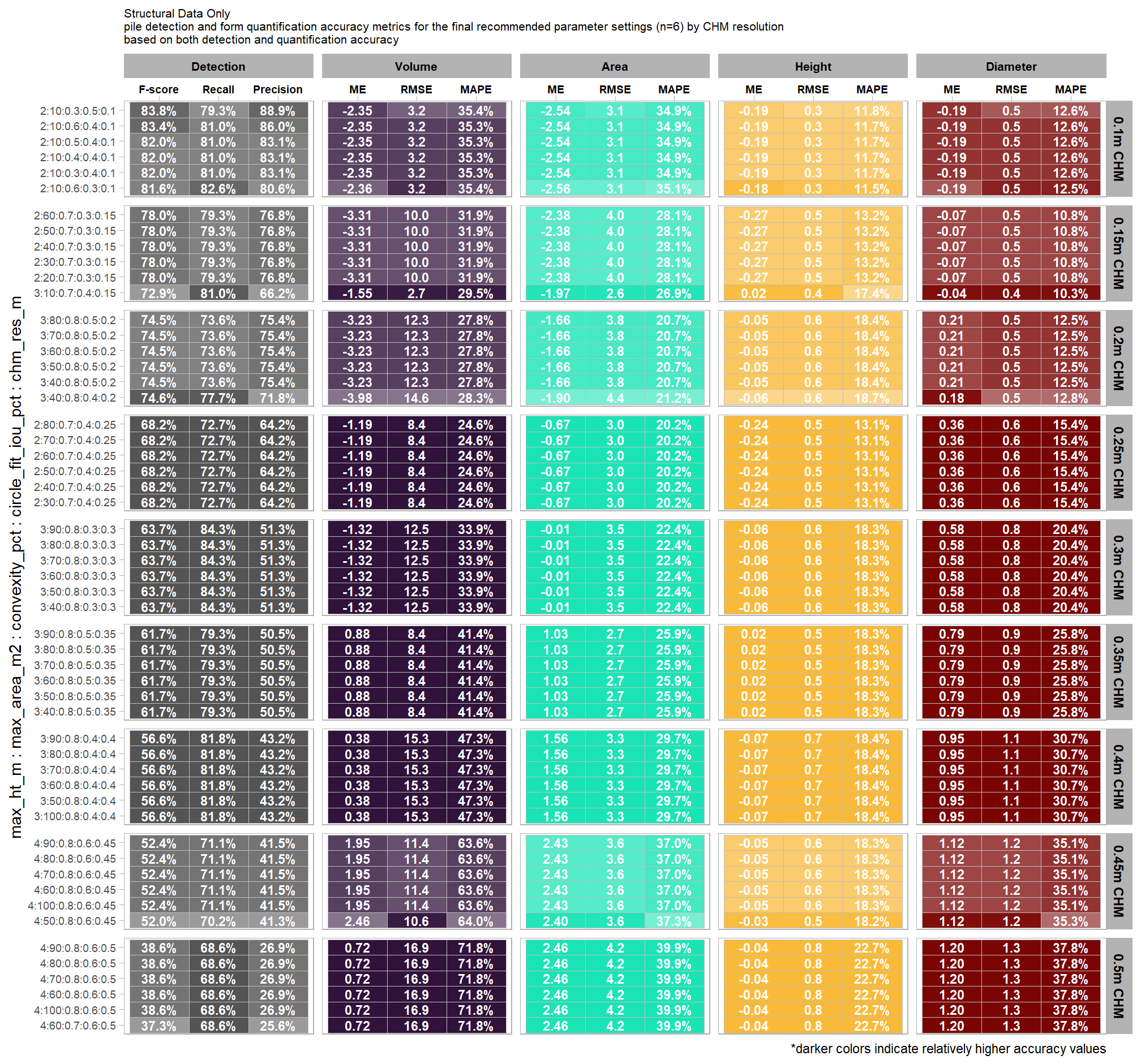
Posterior predictive checks were used to evaluate model goodness-of-fit by comparing data simulated from the model with the observed data used to estimate the model parameters (Hobbs & Hooten, 2015). Calculating the proportion of MCMC iterations in which the test statistic (i.e., mean and sum of squares) from the simulated data and observed data are more extreme than one another provides the Bayesian p-value. Lack of fit is indicated by a value close to 0 or 1 while a value of 0.5 indicates perfect fit (Hobbs & Hooten, 2015).
To learn more about this approach to posterior predictive checks, check out Gabry’s (2025) vignette, Graphical posterior predictive checks using the bayesplot package.
posterior-predictive check to make sure the model does an okay job simulating data that resemble the sample data. our objective is to construct the model such that it faithfully represents the data.
# posterior predictive check
brms::pp_check(
brms_diam_mape_mod
, type = "dens_overlay"
, ndraws = 100
) +
ggplot2::labs(subtitle = "posterior-predictive check (overlaid densities)") +
ggplot2::theme_light() +
ggplot2::scale_y_continuous(NULL, breaks = NULL) +
ggplot2::theme(
legend.position = "top", legend.direction = "horizontal"
, legend.text = ggplot2::element_text(size = 14)
, plot.subtitle = ggplot2::element_text(size = 8)
, plot.title = ggplot2::element_text(size = 9)
)
another way
brms::pp_check(brms_diam_mape_mod, type = "ecdf_overlay", ndraws = 100) +
ggplot2::labs(subtitle = "posterior-predictive check (ECDF: empirical cumulative distribution function)") +
ggplot2::theme_light() +
ggplot2::theme(
legend.position = "top", legend.direction = "horizontal"
, legend.text = ggplot2::element_text(size = 14)
)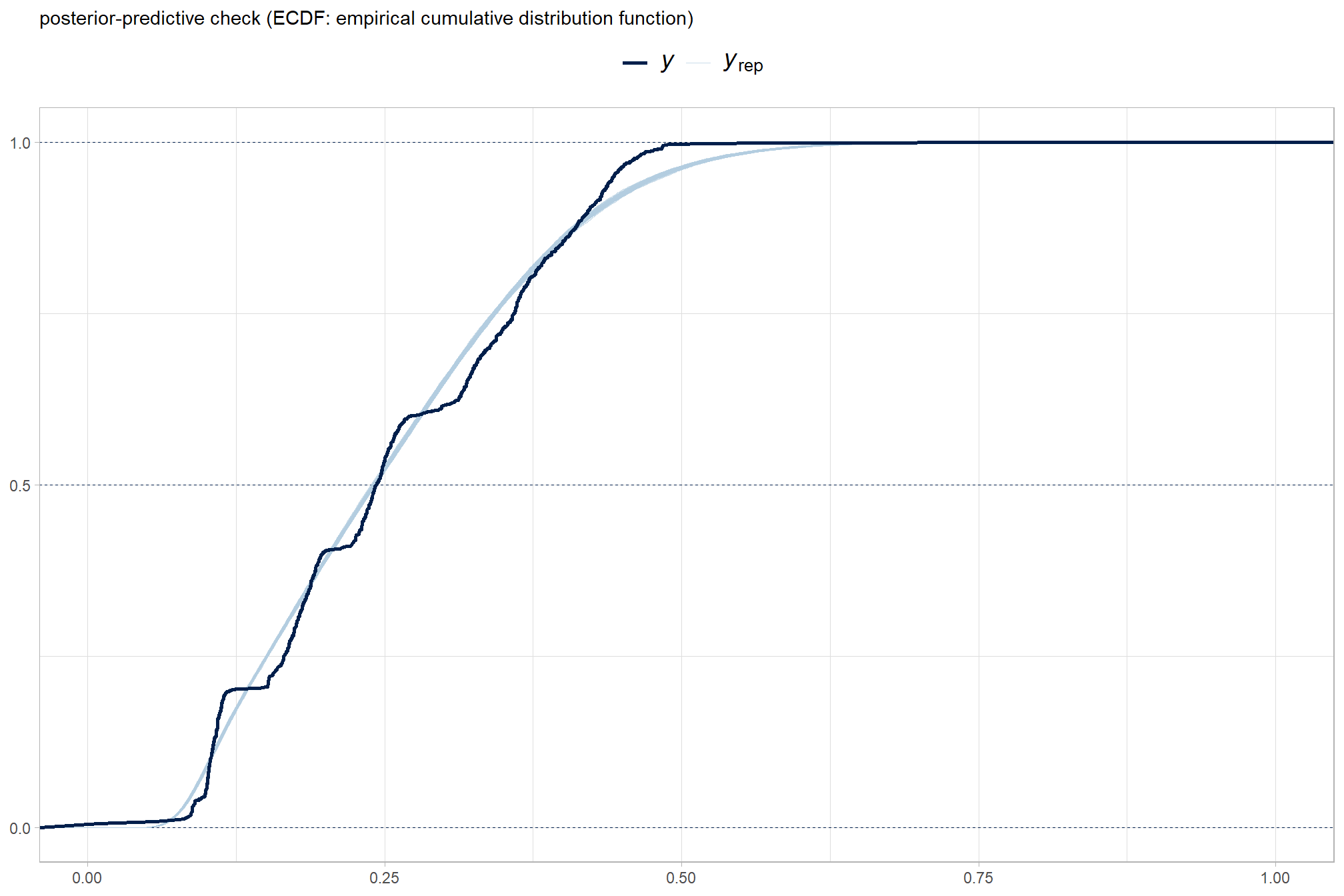
9.2.4 Conditional Effects
first, lets look at densities of the posterior samples per parameter
brms::mcmc_plot(brms_diam_mape_mod, type = "dens") +
# ggplot2::theme_light() +
ggplot2::theme(
strip.text = ggplot2::element_text(size = 7.5, face = "bold", color = "black")
)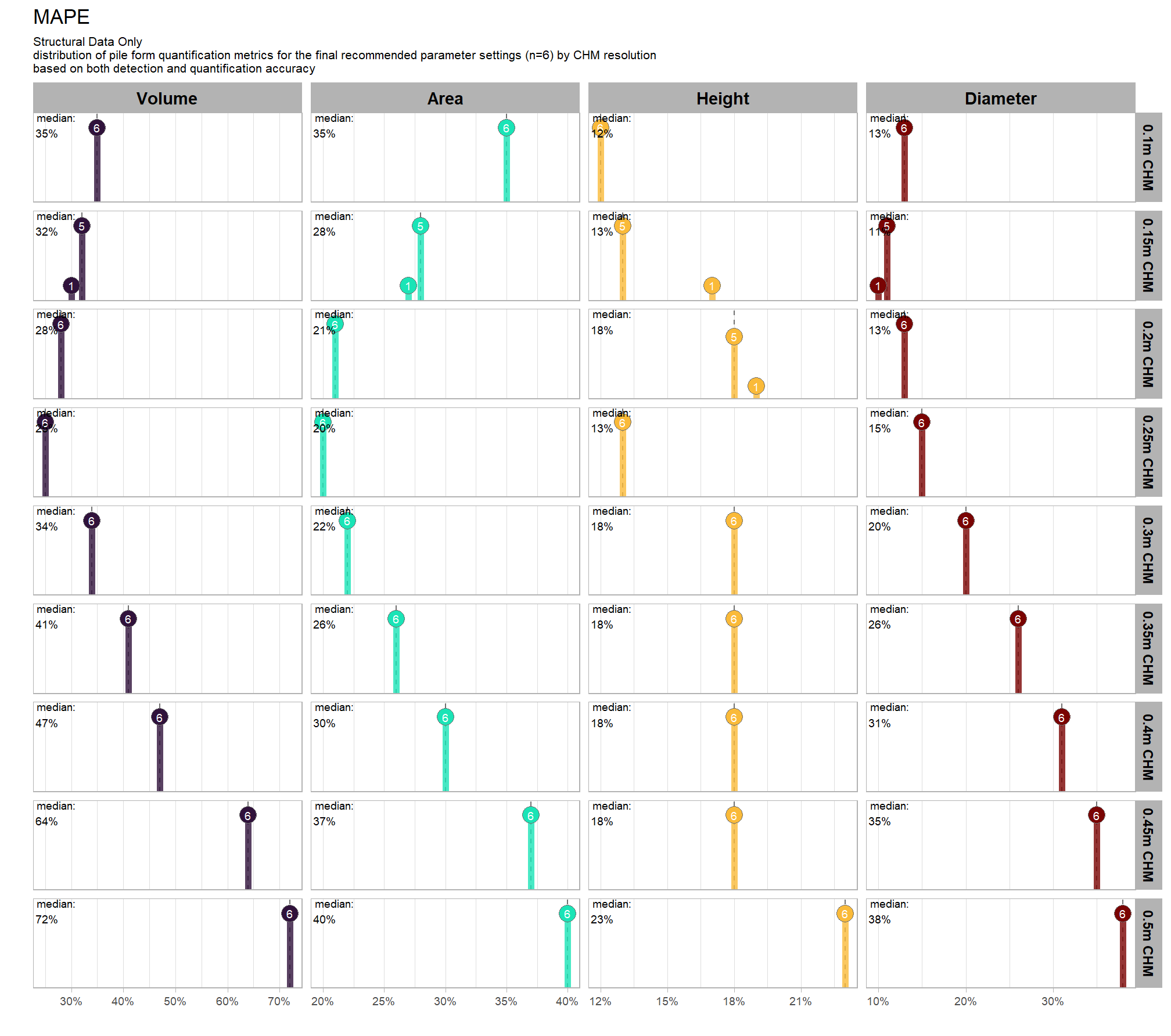
and we can look at the default coefficient plot that is commonly used in reporting coefficient “significance” in frequentist analysis
# easy way to get the default coeff plot
brms::mcmc_plot(brms_diam_mape_mod, variable = "\\bb_", regex = T, type = "intervals")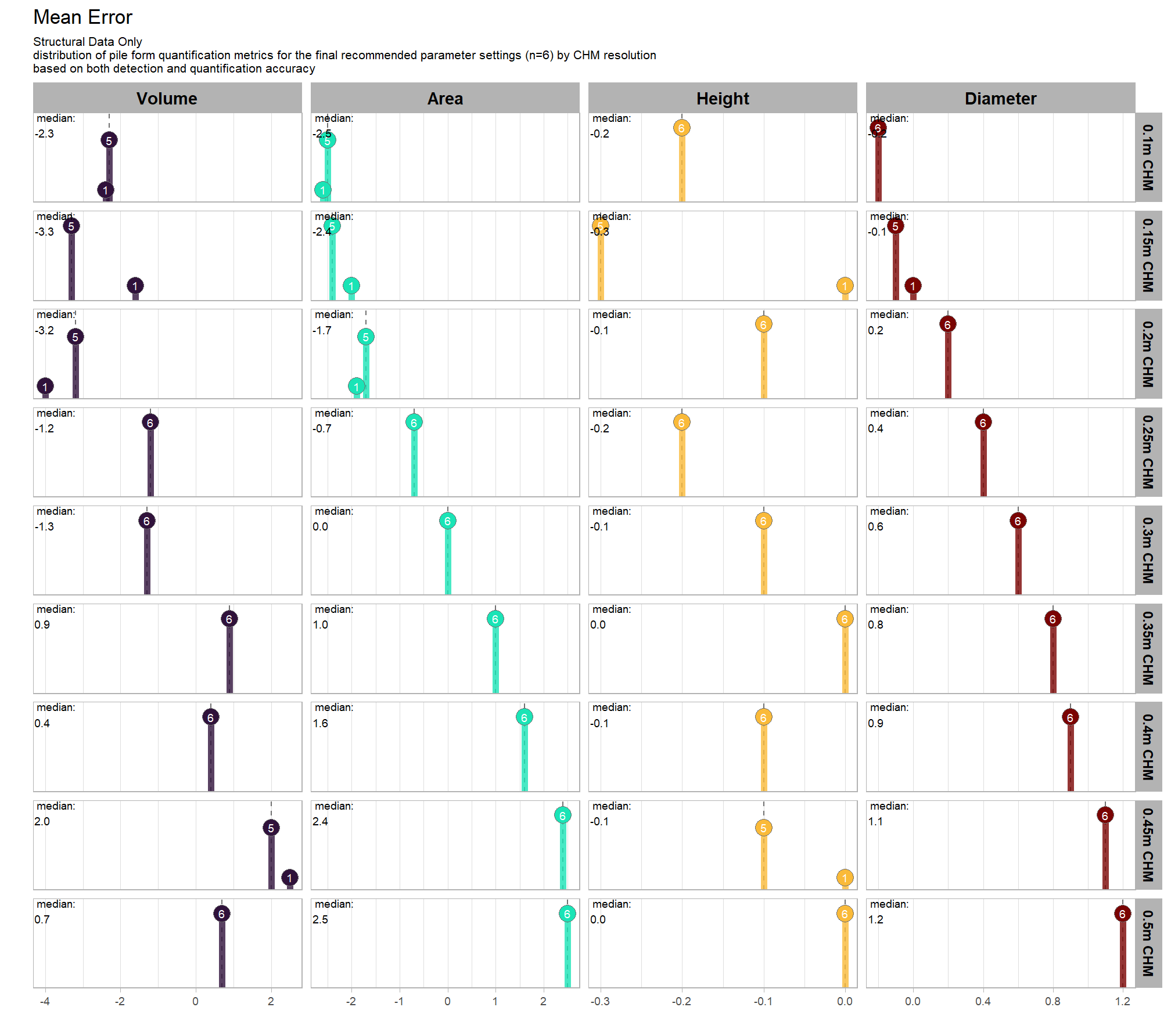
Regarding interactions and polynomial models like the one we use, McElreath (2015) notes:
parameters are the linear and square components of the curve, respectively. But that doesn’t make them transparent. You have to plot these model fits to understand what they are saying. (p. 112-113)
all of the interactions and the quadradic trend of this model combine to make these coefficients by themselves uninterpretable as the coefficients are only meaningful in the context of the other terms in the interaction or by adding the quadratic component
we can do this by checking for the main effects of the individual variables on F-score (averages across all other effects)
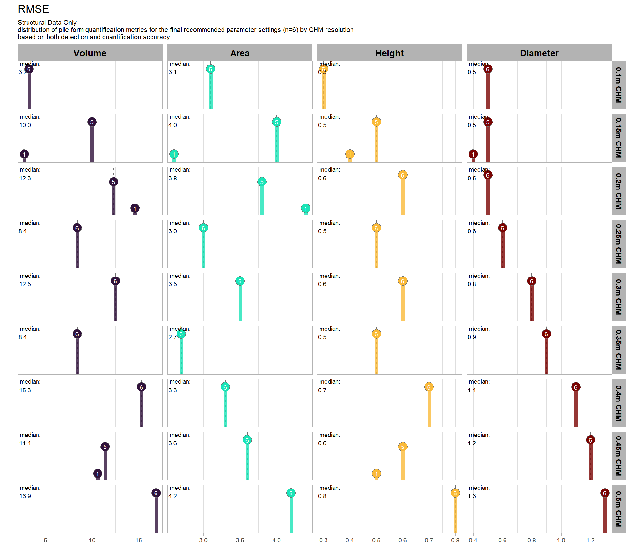
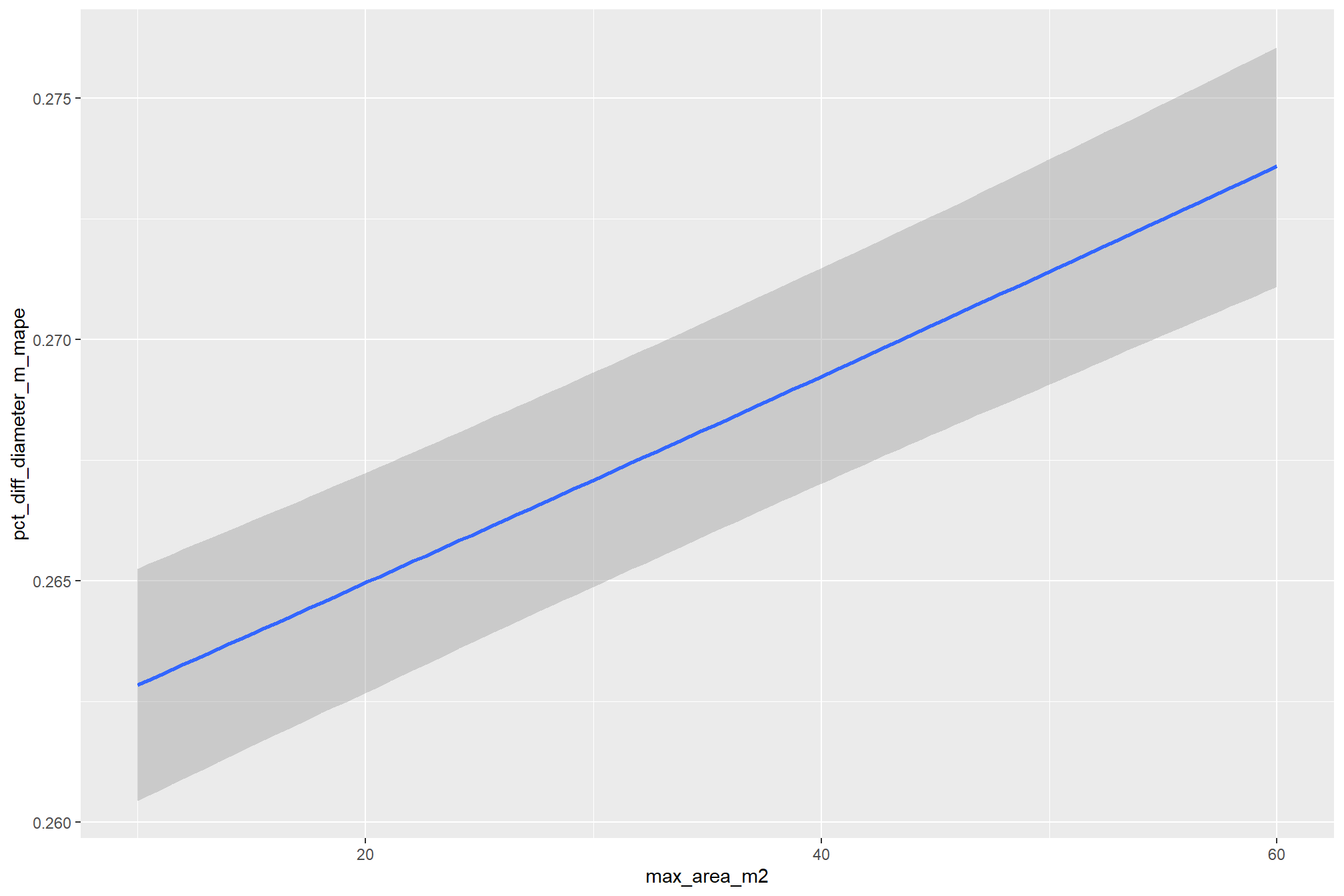
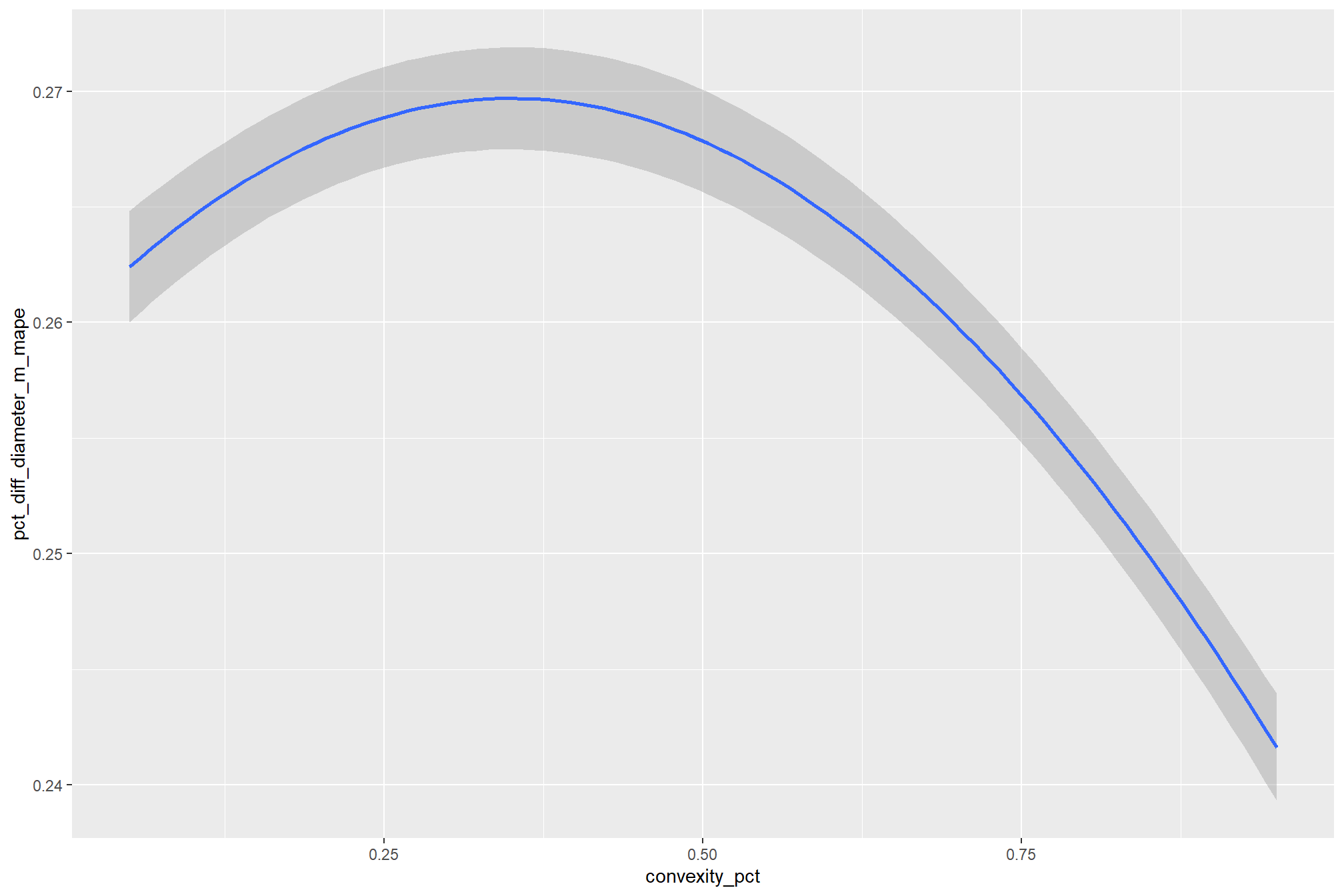
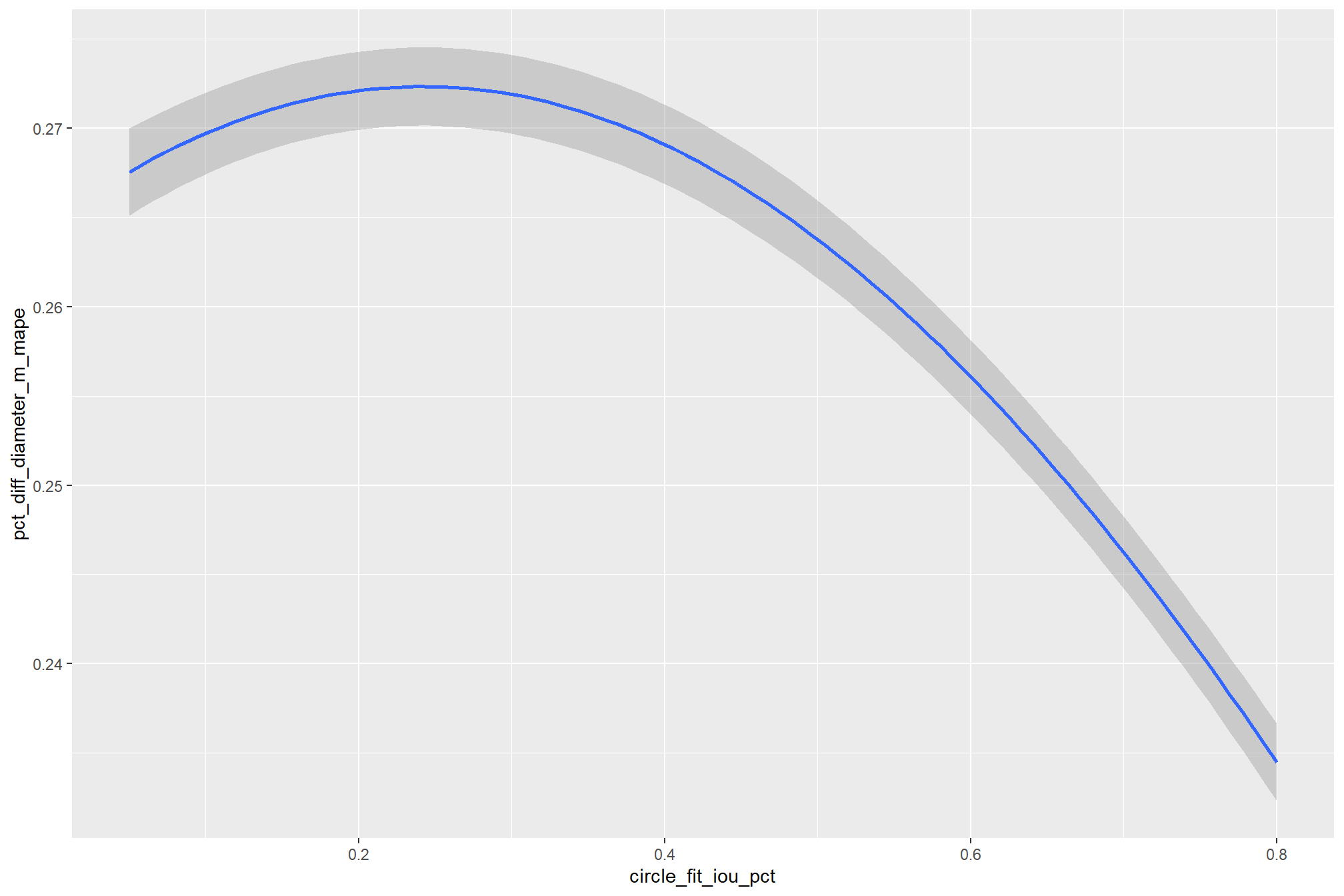
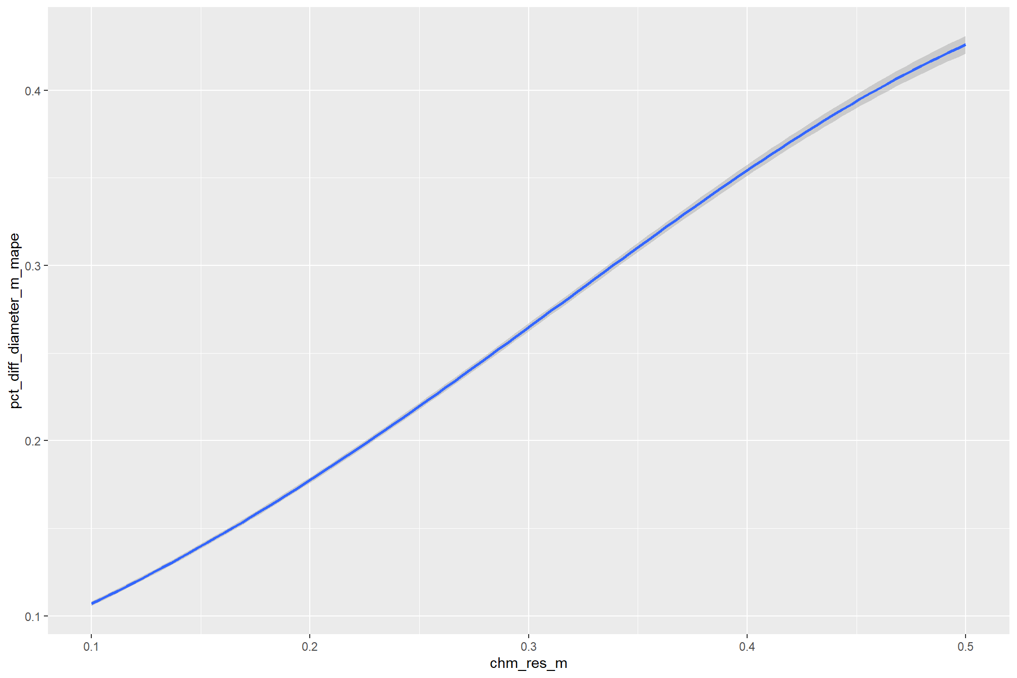
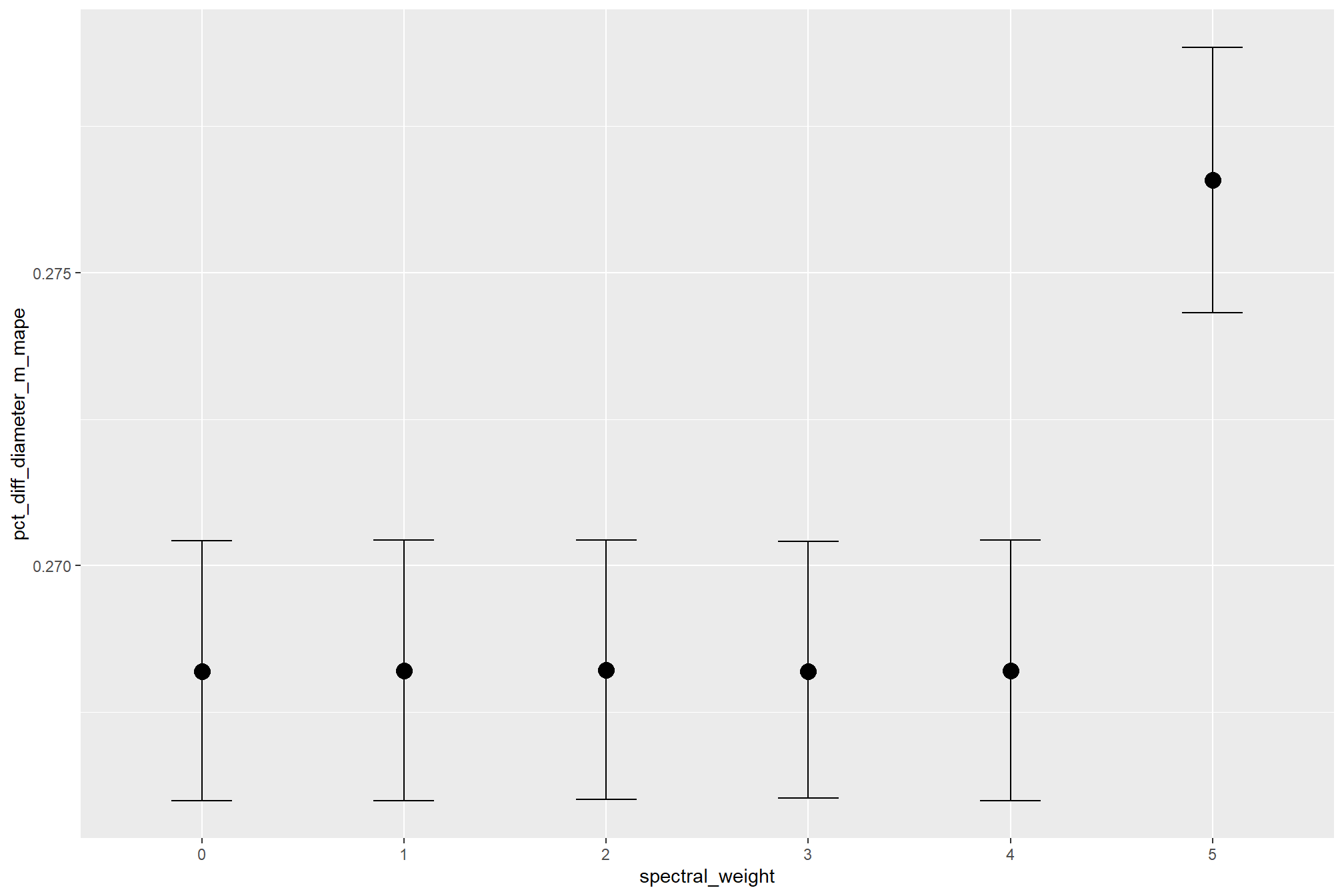
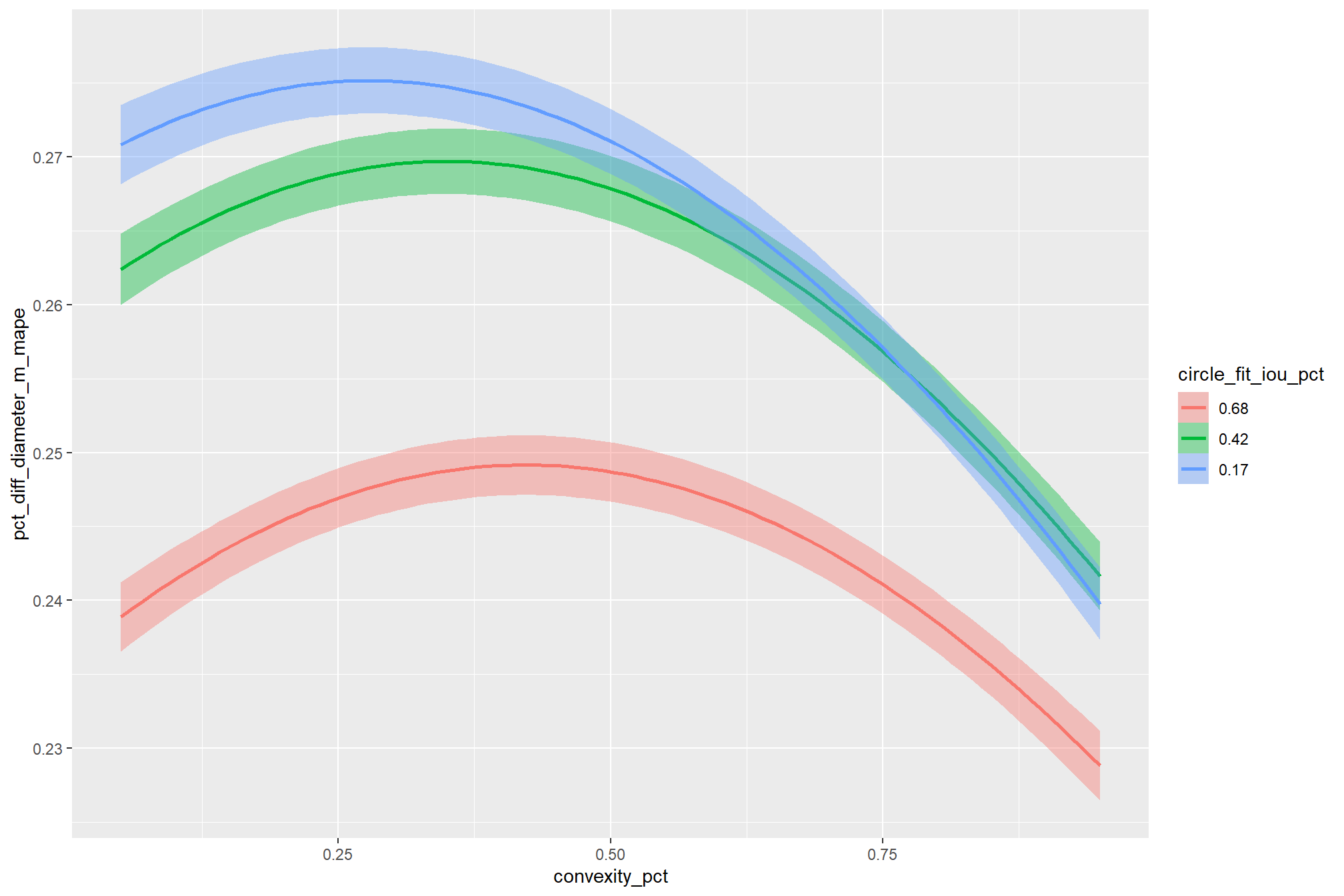
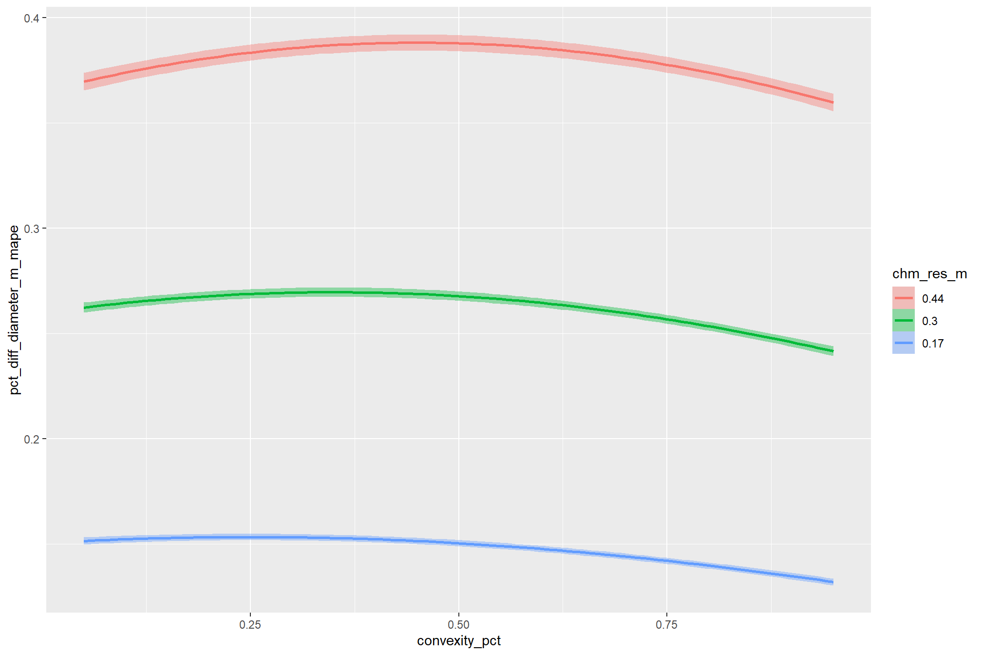

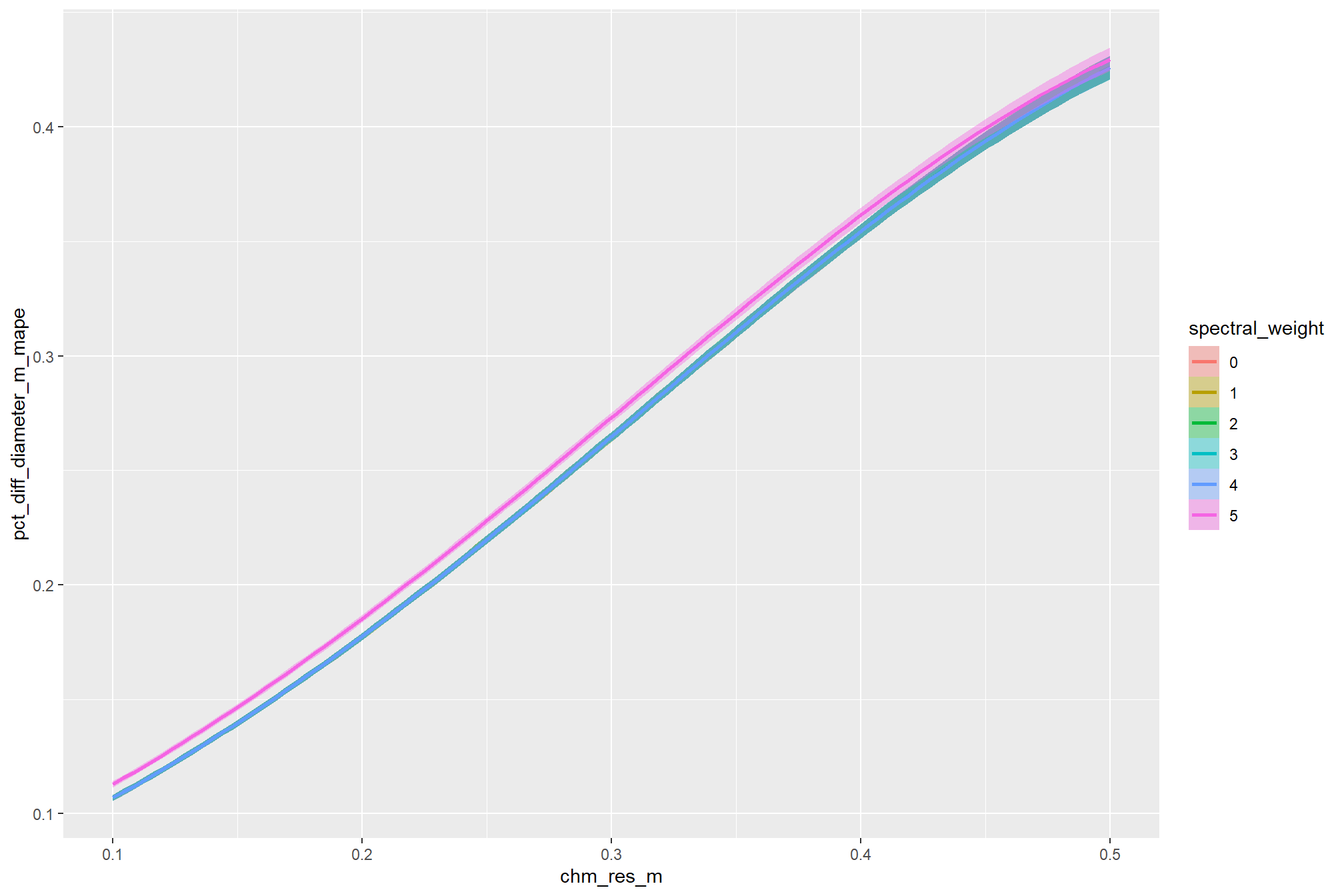
9.2.5 Posterior Predictive Expectation
we will test our hypotheses using the posterior distributions of the expected values (i.e., the posterior predictions of the mean) obtained via tidybayes::add_epred_draws(). our analysis will include two stages using parameter levels of the four structural parameters: max_ht_m, max_area_m2, convexity_pct, circle_fit_iou_pct. in practice, these values should be informed by the treatment prescription implemented on the ground.
In the first stage, we will fix the max_ht_m and max_area_m2 parameters at levels expected based on the treatment and slash pile construction prescription implemented on the ground. We will then explore the influence of the two geometric shape filtering parameters (circle_fit_iou_pct and convexity_pct) over different levels of the spectral_weight parameter and CHM resolution data.
In the second stage, we will fix all four structural parameters (max_ht_m, max_area_m2, convexity_pct, circle_fit_iou_pct) to explore the influence of the input data, which includes the presence or absence of spectral data and its weighting (i.e. spectral_weight) as well as the CHM resolution (chm_res_m). As in the first stage, the max_ht_m, max_area_m2 parameters will be fixed at expected levels based on the slash pile construction prescription while the convexity_pct, circle_fit_iou_pct are fixed at the optimal levels determined based on the Bayesian posterior predictive distribution of detection accuracy
as a reminder, here are those parameter levels
## Rows: 1
## Columns: 4
## $ circle_fit_iou_pct <dbl> 0.35
## $ convexity_pct      <dbl> 0.36
## $ max_ht_m           <dbl> 2.3
## $ max_area_m2 <dbl> 46now we’ll get the posterior predictive draws but over a range of circle_fit_iou_pct and convexity_pct including the best setting
seq_temp <- seq(from = 0.05, to = 1.0, by = 0.1)
seq2_temp <- seq_temp[seq(1, length(seq_temp), by = 2)] # get every other element
# draws
draws_temp <-
# get the draws for levels of
# spectral_weight circle_fit_iou_pct convexity_pct
tidyr::crossing(
param_combos_spectral_ranked %>% dplyr::distinct(spectral_weight)
, circle_fit_iou_pct = seq_temp %>% unique()
, convexity_pct = seq_temp %>% unique()
, chm_res_m = seq(from = 0.1, to = 1.0, by = 0.1)
, max_ht_m = structural_params_settings$max_ht_m
, max_area_m2 = structural_params_settings$max_area_m2
) %>%
# dplyr::glimpse()
tidybayes::add_epred_draws(brms_diam_mape_mod, ndraws = 1111) %>%
dplyr::rename(value = .epred) %>%
dplyr::mutate(
is_seq = (convexity_pct %in% seq_temp) & (circle_fit_iou_pct %in% seq_temp)
)
# # huh?
draws_temp %>% dplyr::glimpse()## Rows: 6,666,000
## Columns: 12
## Groups: spectral_weight, circle_fit_iou_pct, convexity_pct, chm_res_m, max_ht_m, max_area_m2, .row [6,000]
## $ spectral_weight <fct> 0, 0, 0, 0, 0, 0, 0, 0, 0, 0, 0, 0, 0, 0, 0, 0, 0, …
## $ circle_fit_iou_pct <dbl> 0.05, 0.05, 0.05, 0.05, 0.05, 0.05, 0.05, 0.05, 0.0…
## $ convexity_pct <dbl> 0.05, 0.05, 0.05, 0.05, 0.05, 0.05, 0.05, 0.05, 0.0…
## $ chm_res_m <dbl> 0.1, 0.1, 0.1, 0.1, 0.1, 0.1, 0.1, 0.1, 0.1, 0.1, 0…
## $ max_ht_m <dbl> 2.3, 2.3, 2.3, 2.3, 2.3, 2.3, 2.3, 2.3, 2.3, 2.3, 2…
## $ max_area_m2 <dbl> 46, 46, 46, 46, 46, 46, 46, 46, 46, 46, 46, 46, 46,…
## $ .row <int> 1, 1, 1, 1, 1, 1, 1, 1, 1, 1, 1, 1, 1, 1, 1, 1, 1, …
## $ .chain <int> NA, NA, NA, NA, NA, NA, NA, NA, NA, NA, NA, NA, NA,…
## $ .iteration <int> NA, NA, NA, NA, NA, NA, NA, NA, NA, NA, NA, NA, NA,…
## $ .draw <int> 1, 2, 3, 4, 5, 6, 7, 8, 9, 10, 11, 12, 13, 14, 15, …
## $ value <dbl> 0.1045783, 0.1045749, 0.1026696, 0.1045097, 0.10403…
## $ is_seq <lgl> TRUE, TRUE, TRUE, TRUE, TRUE, TRUE, TRUE, TRUE, TRU…9.2.5.1 Geometric shape regularity
let’s look at the influence of the parameters that control the geometric shape regularity filtering: circle_fit_iou_pct and convexity_pct. to do this, we will fix the max_ht_m and max_area_m2 parameters at levels expected based on the treatment and slash pile construction prescription implemented on the ground.
In the first stage, we will fix the max_ht_m and max_area_m2 parameters at levels expected based on the treatment and slash pile construction prescription implemented on the ground. We will then explore the influence of the two geometric shape filtering parameters (circle_fit_iou_pct and convexity_pct) over different levels of the spectral_weight parameter and CHM resolution data.
In the second stage, we will fix all four structural parameters (max_ht_m, max_area_m2, convexity_pct, circle_fit_iou_pct) to explore the influence of the input data, which includes the presence or absence of spectral data and its weighting (i.e. spectral_weight) as well as the CHM resolution (chm_res_m). As in the first stage, the max_ht_m, max_area_m2 parameters will be fixed at expected levels based on the slash pile construction prescription while the convexity_pct, circle_fit_iou_pct will be fixed at the optimal levels determined based on the Bayesian posterior predictive distribution of detection accuracy
9.2.5.1.1 circle_fit_iou_pct
we need to look at the influence of circle_fit_iou_pct in the context of the other terms in the interaction
draws_temp %>%
dplyr::ungroup() %>%
dplyr::filter(
is_seq
, chm_res_m %in% seq(0.1,0.5,by=0.2)
, convexity_pct %in% seq2_temp
) %>%
dplyr::mutate(convexity_pct = factor(convexity_pct, ordered = T)) %>%
ggplot2::ggplot(mapping = ggplot2::aes(x = circle_fit_iou_pct, y = value, color = convexity_pct)) +
tidybayes::stat_lineribbon(
point_interval = "median_hdi", .width = c(0.95)
, lwd = 1.1, fill = NA
) +
ggplot2::facet_grid(cols = dplyr::vars(spectral_weight), rows = dplyr::vars(chm_res_m), labeller = "label_both", scales = "free_y") +
ggplot2::scale_fill_brewer(palette = "Greys") +
ggplot2::scale_color_viridis_d(option = "mako", begin = 0.6, end = 0.1) +
ggplot2::scale_x_continuous(limits = c(0,1)) +
ggplot2::scale_y_continuous(labels = scales::percent) +
ggplot2::labs(
title = "conditional effect of `circle_fit_iou_pct` on Diameter MAPE"
# , subtitle = "Faceted by spectral_weight and chm_res_m"
, x = "`circle_fit_iou_pct`"
, y = "Diameter MAPE"
, color = "`convexity_pct`"
) +
ggplot2::theme_light() +
ggplot2::theme(
legend.position = "top"
, strip.text.x = ggplot2::element_text(size = 10, color = "black", face = "bold")
, strip.text.y = ggplot2::element_text(size = 10, color = "black", face = "bold")
) +
ggplot2::guides(
color = ggplot2::guide_legend(override.aes = list(shape = 15, lwd = 8, fill = NA))
, fill = "none"
)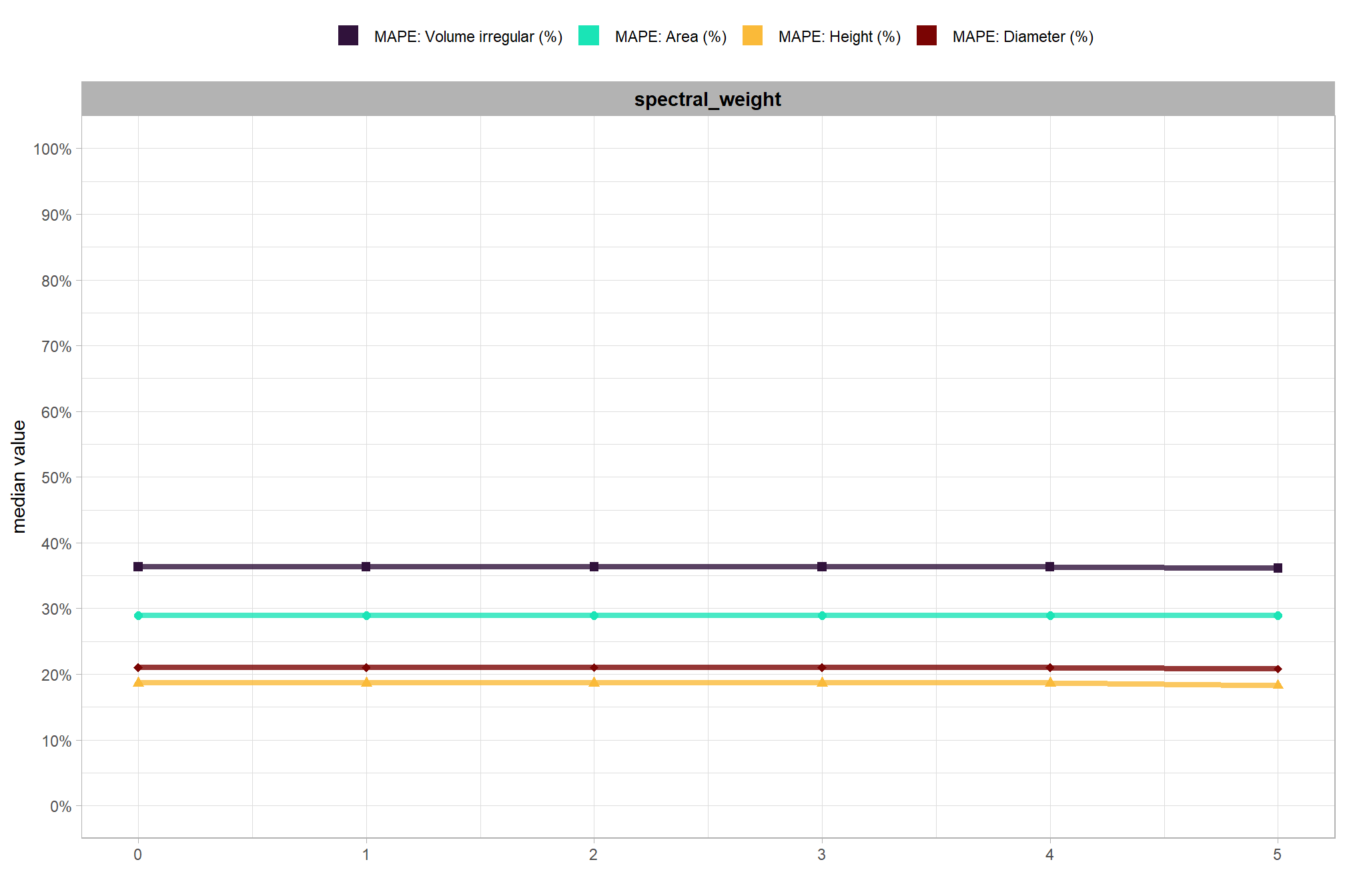
For all of these faceted plots, take note of the narrow range of the y-axis (Predicted Diameter MAPE), which is particularly narrow for finer resolution CHM data (e.g., <0.3m). The non-linear relationship between the circle_fit_iou_pct parameter and the Diameter MAPE is prominent, especially for coarser resolution CHM data. This is confirmed by the statistical model’s negative quadratic coefficient for the squared term of circle_fit_iou_pct (i.e., I(circle_fit_iou_pct^2)), which indicates a downward-opening parabolic shape. Across all CHM resolutions and irrespective of the spectral_weight setting, diameter quantification accuracy is highest (MAPE is lowest) at the highest values of the circle_fit_iou_pct parameter (e.g., greater than 0.6). This finding is intuitive: diameter error is calculated only for True Positive matches, and when a successful match is made between a prediction and a ground truth pile at these high circularity thresholds, it strongly suggests the predicted pile perimeter accurately conforms to the ground truth pile shape.
The influence of the circle_fit_iou_pct parameter on diameter accuracy is conditional on the convexity_pct parameter setting. The relationship between these parameters is most evident with coarser resolution CHM data (e.g., >0.3m) and looking at cases when convexity_pct parameter is set low (e.g., less than 0.4) the best diameter quantification accuracy occurs when the circle_fit_iou_pct parameter is set high (e.g., greater than 0.5), and vice-versa. This effect occurs because both parameters function as geometric shape filters in the rules-based methodology. When the piles in the treatment area are generally uniform (e.g., mostly circular), the parameters become somewhat redundant. However, when pile shapes are heterogeneous, these two filtering parameters must be balanced to fine-tune the retention of objects. For instance, if piles are expected to be rectangular, the optimal setting would be to effectively disable the circle_fit_iou_pct filter (i.e., set it to ‘0’) and rely on the convexity_pct filter to retain objects with the expected perimeter regularity.
Finally, the circle_fit_iou_pct parameter has a smaller influence on diameter quantification accuracy with finer resolution CHM data (e.g., <0.3m) and a larger influence on Diameter MAPE for coarser CHM data (e.g., >0.3m). For the coarser CHM data, increasing values of the circle_fit_iou_pct parameter on the right side of the vertex increased diameter quantification accuracy (decreased MAPE) at an increasing rate as the parameter approached ‘1’.
9.2.5.1.2 convexity_pct
we need to look at the influence of convexity_pct in the context of the other terms in the interaction
draws_temp %>%
dplyr::ungroup() %>%
dplyr::filter(
is_seq
, chm_res_m %in% seq(0.1,0.5,by=0.2)
, circle_fit_iou_pct %in% seq2_temp
) %>%
dplyr::mutate(circle_fit_iou_pct = factor(circle_fit_iou_pct, ordered = T)) %>%
ggplot2::ggplot(mapping = ggplot2::aes(x = convexity_pct, y = value, color = circle_fit_iou_pct)) +
tidybayes::stat_lineribbon(
point_interval = "median_hdi", .width = c(0.95)
, lwd = 1.1
, fill = NA
) +
ggplot2::facet_grid(cols = dplyr::vars(spectral_weight), rows = dplyr::vars(chm_res_m), labeller = "label_both", scales = "free_y") +
ggplot2::scale_fill_brewer(palette = "Greys") +
ggplot2::scale_color_viridis_d(option = "magma", begin = 0.5, end = 0.1) +
ggplot2::scale_x_continuous(limits = c(0,1)) +
ggplot2::scale_y_continuous(labels = scales::percent) +
ggplot2::labs(
title = "conditional effect of `convexity_pct` on Diameter MAPE"
# , subtitle = "Faceted by spectral_weight and chm_res_m"
, x = "`convexity_pct`"
, y = "Diameter MAPE"
, color = "`circle_fit_iou_pct`"
) +
ggplot2::theme_light() +
ggplot2::theme(
legend.position = "top"
, strip.text.x = ggplot2::element_text(size = 10, color = "black", face = "bold")
, strip.text.y = ggplot2::element_text(size = 10, color = "black", face = "bold")
) +
ggplot2::guides(
color = ggplot2::guide_legend(override.aes = list(shape = 15, lwd = 8, fill = NA))
, fill = "none"
)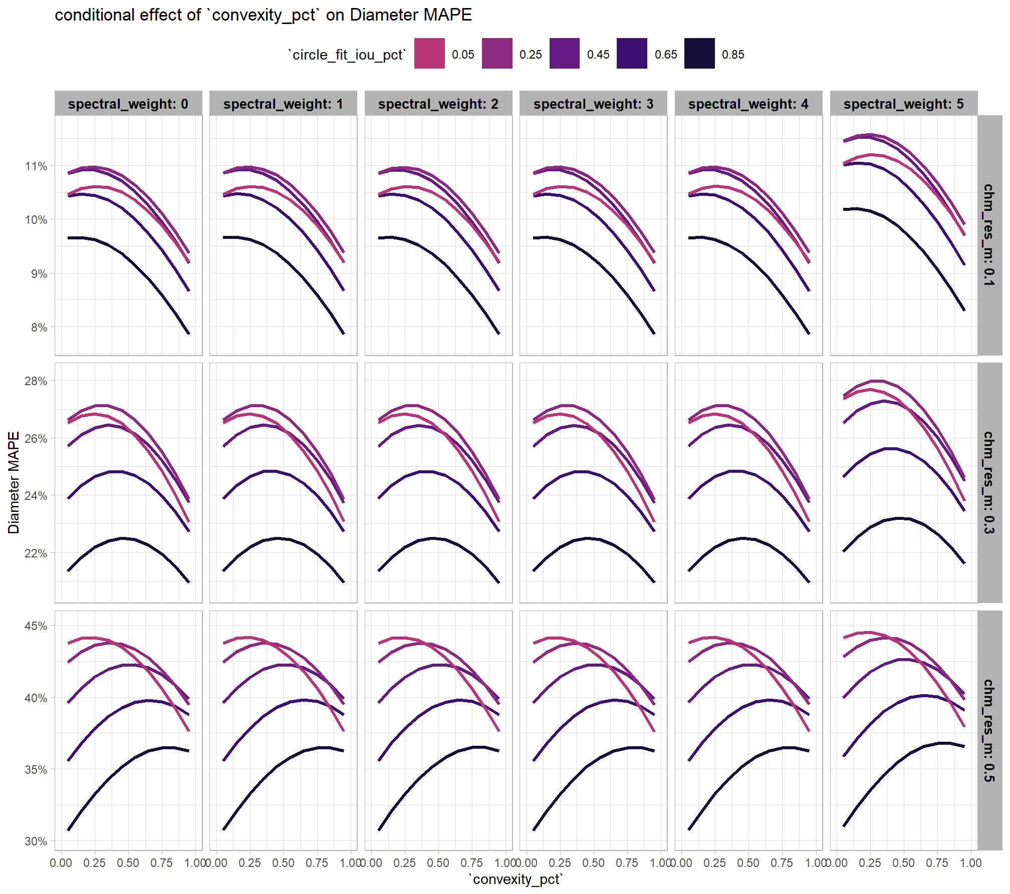
The model shows that the influence of the convexity_pct parameter on the Diameter MAPE is conditional on the CHM resolution. The magnitude of this influence varies significantly: for finer resolution CHM data (e.g., less than 0.3m), the convexity_pct parameter has a minimal impact on the Diameter MAPE, as evidenced by the narrow range of the y-axis; conversely, its influence is considerably larger at coarser resolutions. Across all CHM resolutions tested, it is clear that the influence of the circle_fit_iou_pct parameter on diameter accuracy is conditional on the convexity_pct parameter setting. This relationship is most pronounced with coarser resolution CHM data (e.g., greater than 0.3m). For example, using 0.5m CHM data, the vertex of the downward-opening parabola (which indicates the largest diameter quantification error) shifts across the convexity_pct range: it is located at lower convexity_pct values (i.e., less than 0.5) when the circle_fit_iou_pct parameter is set low (e.g., less than 0.4), but shifts to higher convexity_pct values (i.e., greater than 0.6) when the circle_fit_iou_pct parameter is set high (e.g., greater than 0.6). This inverse relationship occurs because both parameters function as geometric shape filters in the rules-based methodology. For the test data, where piles generally exhibit regular, circular footprints, the two filters become somewhat redundant. Therefore, the lowest Diameter MAPE (highest accuracy) is achieved when the parameters are complementary: when circle_fit_iou_pct is high (near 1) and convexity_pct is low (near 0), or vice-versa. Additionally, if circle_fit_iou_pct is at an intermediate level (near 0.5), convexity_pct should be set either high or low to maintain diameter quantification accuracy. It is important to note though, that these relationships are specific to regularly shaped circular pile footprints; if pile bases are expected to be square or rectangular, the parameters should be rebalanced. For instance, in a scenario predicting rectangular piles, the optimal setting would be to effectively disable the circle_fit_iou_pct filter (set to ‘0’) and instead rely on the convexity_pct filter to enforce the expected shape regularity filtering.
9.2.5.1.3 Optimizing geometric filtering
Given the complexity of our model, which includes a non-linear link function and parameter interactions, calculating the optimal parameter values by solving for them algebraically from the model’s coefficients would be prone to error. instead, we can use a robust Bayesian approach that leverages the model’s posterior predictive distribution. This method is powerful because it inherently accounts for all sources of model uncertainty.
first, we’ll generate a large number of predictions across a fine grid of parameter values (e.g. in steps of 0.01) for each posterior draw of the model coefficients. we’ll generate a large number (e.g. 1000+) of posterior predictive draws for each combination of parameter values. for each posterior predictive draw, we’ll then identify the parameter combination that maximizes the Diameter MAPE and we’ll be left with a posterior distribution of optimal parameter combinations.
this approach demonstrates a key advantage of the Bayesian framework, allowing us to ask complex questions and find the most probable optimal parameter combination while fully accounting for uncertainty.
note, we only extract draws based on not using any spectral data (i.e. spectral_weight = 0) to save on plotting space and because we expect form quantification to only be minimally influenced by the inclusion of spectral data
# let's get the draws at a very granular level
vertex_draws_temp <-
tidyr::crossing(
param_combos_spectral_ranked %>%
dplyr::filter(spectral_weight=="0") %>%
dplyr::distinct(spectral_weight, spectral_weight_fact)
, circle_fit_iou_pct = seq(from = 0.0, to = 1, by = 0.01) # very granular to identify vertex
, convexity_pct = seq(from = 0.0, to = 1, by = 0.02) # very granular to identify vertex
, chm_res_m = seq(0.1,0.5,by=0.1)
, max_ht_m = structural_params_settings$max_ht_m
, max_area_m2 = structural_params_settings$max_area_m2
) %>%
tidybayes::add_epred_draws(brms_diam_mape_mod, ndraws = 1000, value = "value") %>%
dplyr::ungroup() %>%
# for each draw, get the highest Diameter MAPE by chm_res_m, spectral_weight
# which we'll use to identify the optimal circle_fit_iou_pct,convexity_pct settings
# these are essentially "votes" based on likelihood
dplyr::group_by(
.draw
, chm_res_m, spectral_weight
) %>%
dplyr::arrange(value,circle_fit_iou_pct,convexity_pct) %>% # notice the ascending sort of value (mape) here to take the lowest
dplyr::slice(1)
# vertex_draws_temp %>% dplyr::glimpse() # this thing is hugeplot the posterior distribution of optimal parameter setting for circle_fit_iou_pct
vertex_draws_temp %>%
dplyr::filter(
chm_res_m %in% seq(0.1,0.5,by=0.1)
) %>%
dplyr::ungroup() %>%
ggplot2::ggplot(mapping = ggplot2::aes(x = circle_fit_iou_pct)) +
tidybayes::stat_dotsinterval(
point_interval = "median_hdci", .width = c(0.95)
, quantiles = 100
, point_size = 3
) +
ggplot2::facet_grid(
cols = dplyr::vars(spectral_weight)
, rows = dplyr::vars(chm_res_m)
, scales = "free_y"
, labeller = "label_both"
, axes = "all_x"
) +
# ggplot2::scale_x_continuous(limits = c(0,1)) +
ggplot2::scale_x_continuous(limits = c(0,1), breaks = scales::breaks_extended(6)) +
ggplot2::scale_y_continuous(NULL, breaks = NULL) +
ggplot2::theme_light() +
ggplot2::theme(
strip.text.x = ggplot2::element_text(size = 10, color = "black", face = "bold")
, strip.text.y = ggplot2::element_text(size = 8, color = "black", face = "bold")
, axis.text.x = ggplot2::element_text(size = 8)
)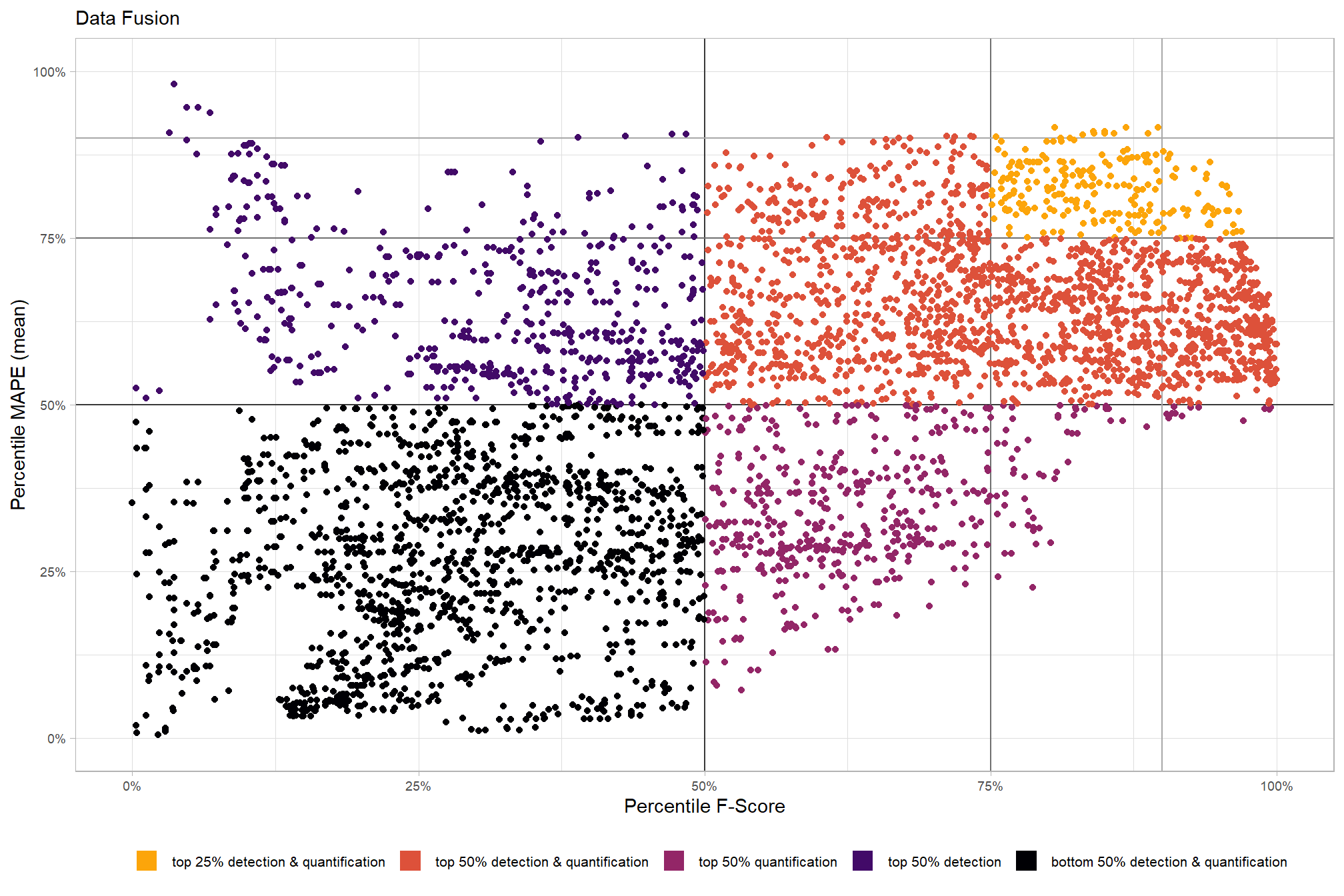
The optimal circle_fit_iou_pct setting for maximizing diameter quantification accuracy is predicted to be near it’s highest setting of ‘1’. This finding is likely not very applicable in real-world scenarios but it is intuitive: diameter error is calculated only for True Positive matches, and when a successful match is made between a prediction and a ground truth pile at these high circularity thresholds, it strongly suggests the predicted pile perimeter accurately conforms to the ground truth pile shape.
plot the posterior distribution of optimal parameter setting for convexity_pct
vertex_draws_temp %>%
dplyr::filter(
chm_res_m %in% seq(0.1,0.5,by=0.1)
) %>%
dplyr::ungroup() %>%
ggplot2::ggplot(mapping = ggplot2::aes(x = convexity_pct)) +
tidybayes::stat_dotsinterval(
point_interval = "median_hdci", .width = c(0.95)
, quantiles = 100
, point_size = 3
) +
ggplot2::facet_grid(
cols = dplyr::vars(spectral_weight)
, rows = dplyr::vars(chm_res_m)
, scales = "free_y"
, labeller = "label_both"
, axes = "all_x"
) +
ggplot2::scale_x_continuous(limits = c(0,1), breaks = scales::breaks_extended(6)) +
ggplot2::scale_y_continuous(NULL, breaks = NULL) +
ggplot2::theme_light() +
ggplot2::theme(
strip.text.x = ggplot2::element_text(size = 10, color = "black", face = "bold")
, strip.text.y = ggplot2::element_text(size = 8, color = "black", face = "bold")
)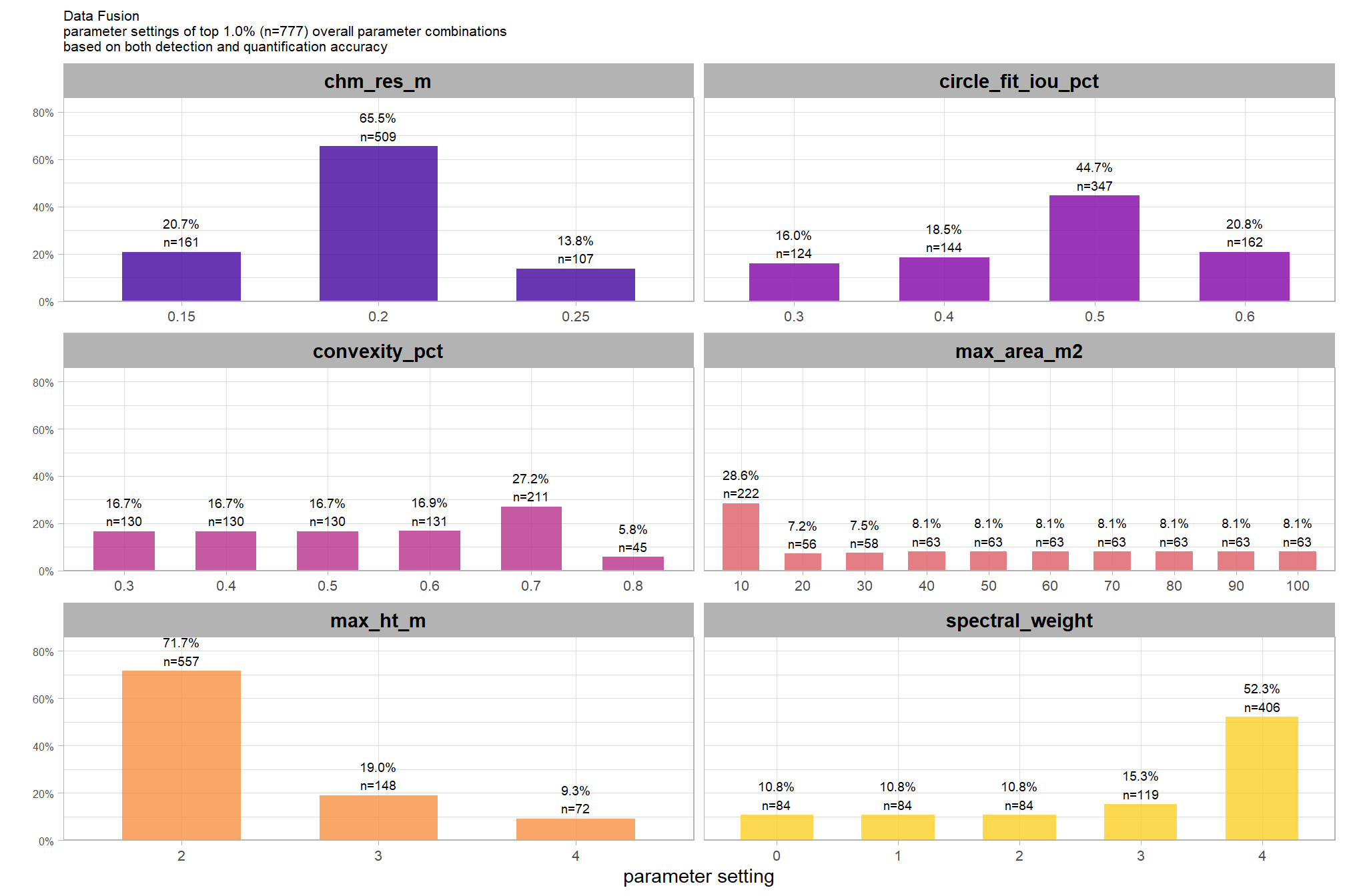
when the circle_fit_iou_pct parameter is optimized (i.e. set near ‘1’), the influence of convexity_pct on form quantification accuracy is dependent on the CHM resolution. only for the finest resolution CHM data (i.e. 0.1m) tested, the model’s predictions indicate with high certainty that the optimal convexity_pct is its maximum value of ‘1’. for coarser resolution CHM data (e.g. 0.3m), the 95% HDI for the optimal convexity_pct spans the entire 0-1 range, indicating the model is not confident in any specific setting. an important distinction is that this finding of irrelavance for the convexity_pct parameter on diameter quantification is only for cases when circle_fit_iou_pct is already optimized, which, as shown above, was at a level near 1 for this coarser-resolution CHM data. at these higher circle_fit_iou_pct levels , the filtering for irregularly shaped objects is accomplished solely by the circle_fit_iou_pct parameter so the convexity_pct is less important for accurate quantification of predicted diameter. however, when the circle_fit_iou_pct parameter is not optimized or is turned off (e.g., set to 0), convexity_pct becomes a crucial parameter for filtering irregularly shaped objects.
we can look at this another way, check it
vertex_draws_temp %>%
dplyr::filter(
chm_res_m %in% seq(0.1,0.5,by=0.1)
) %>%
dplyr::ungroup() %>%
ggplot2::ggplot(mapping = ggplot2::aes(y = convexity_pct, x = circle_fit_iou_pct)) +
# geom_point(alpha=0.2) +
ggplot2::geom_jitter(alpha=0.2, height = .01, width = 0.0) +
ggplot2::facet_grid(
cols = dplyr::vars(spectral_weight)
, rows = dplyr::vars(chm_res_m)
# , scales = "free_y"
, labeller = "label_both"
) +
# ggplot2::scale_x_continuous(limits = c(0,1)) +
ggplot2::scale_x_continuous(limits = c(0,1)) +
# ggplot2::scale_y_continuous(NULL, breaks = NULL) +
ggplot2::theme_light() +
ggplot2::theme(
strip.text.x = ggplot2::element_text(size = 10, color = "black", face = "bold")
, strip.text.y = ggplot2::element_text(size = 8, color = "black", face = "bold")
)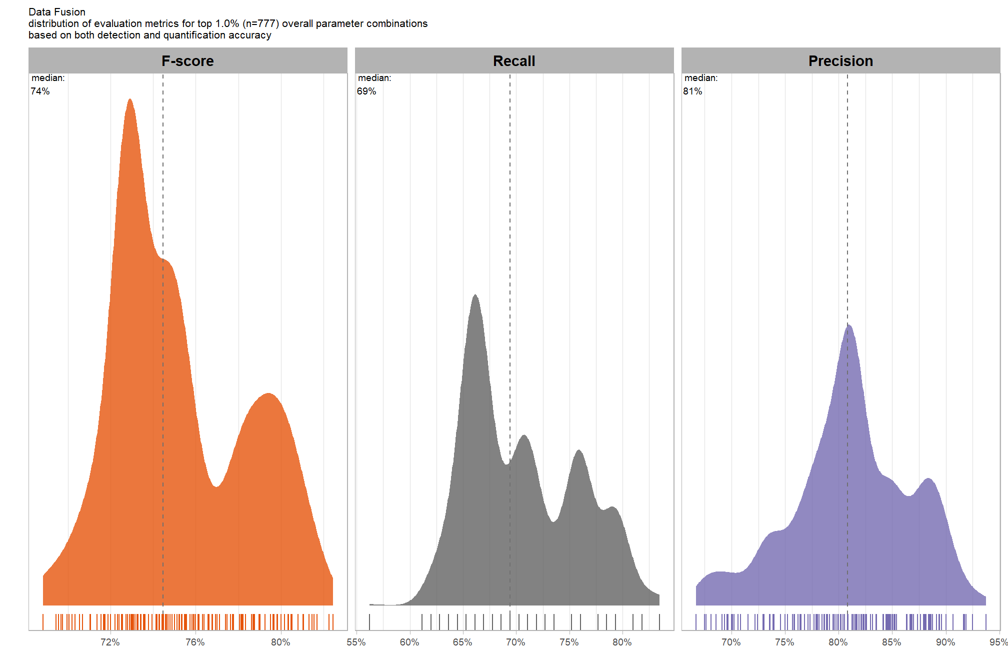
note, in the plot above, we slightly “jitter” the points so that they are visible where they would otherwise be stacked on top of each other and only look like a few points instead of the 1000 draws from the posterior we used
let’s table the HDI of the optimal values
# summarize it
vertex_draws_temp <-
vertex_draws_temp %>%
dplyr::group_by(
chm_res_m, spectral_weight
) %>%
dplyr::summarise(
# get median_hdi
median_hdi_est_circle_fit_iou_pct = tidybayes::median_hdci(circle_fit_iou_pct)$y
, median_hdi_lower_circle_fit_iou_pct = tidybayes::median_hdci(circle_fit_iou_pct)$ymin
, median_hdi_upper_circle_fit_iou_pct = tidybayes::median_hdci(circle_fit_iou_pct)$ymax
# get median_hdi
, median_hdi_est_convexity_pct = tidybayes::median_hdci(convexity_pct)$y
, median_hdi_lower_convexity_pct = tidybayes::median_hdci(convexity_pct)$ymin
, median_hdi_upper_convexity_pct = tidybayes::median_hdci(convexity_pct)$ymax
) %>%
dplyr::ungroup()
# table it
vertex_draws_temp %>%
kableExtra::kbl(
digits = 2
, caption = ""
, col.names = c(
"CHM resolution", "spectral_weight"
, rep(c("median", "HDI low", "HDI high"),2)
)
, escape = F
) %>%
kableExtra::kable_styling() %>%
kableExtra::collapse_rows(columns = 1, valign = "top") %>%
kableExtra::add_header_above(c(
" "=2
, "circle_fit_iou_pct" = 3
, "convexity_pct" = 3
))| CHM resolution | spectral_weight | median | HDI low | HDI high | median | HDI low | HDI high |
|---|---|---|---|---|---|---|---|
| 0.1 | 0 | 1 | 1 | 1 | 1 | 1 | 1 |
| 0.2 | 0 | 1 | 1 | 1 | 1 | 1 | 1 |
| 0.3 | 0 | 1 | 1 | 1 | 0 | 0 | 1 |
| 0.4 | 0 | 1 | 1 | 1 | 0 | 0 | 0 |
| 0.5 | 0 | 1 | 1 | 1 | 0 | 0 | 0 |
9.2.5.2 Input data
to explore the influence of the input data, which includes the presence or absence of spectral data and its weighting (i.e. spectral_weight) as well as the CHM resolution (chm_res_m), we will fix all four structural parameters (max_ht_m, max_area_m2, convexity_pct, circle_fit_iou_pct). the max_ht_m, max_area_m2 parameters will be fixed at expected levels based on the slash pile construction prescription while the convexity_pct, circle_fit_iou_pct will be fixed at the optimal levels determined based on the Bayesian posterior predictive distribution of detection accuracy
we’ll make contrasts of the posterior predictions to probabilistically quantify the influence of the input data (e.g. inclusion of spectral data and it’s weighting and CHM resolution)
let’s get the posterior predictive draws
# structural_params_settings
draws_temp <-
tidyr::crossing(
structural_params_settings
, param_combos_spectral_ranked %>% dplyr::distinct(spectral_weight_fact, spectral_weight)
, param_combos_spectral_ranked %>% dplyr::distinct(chm_res_m)
) %>%
tidybayes::add_epred_draws(brms_diam_mape_mod, ndraws = 1111) %>%
dplyr::rename(value = .epred)
# # huh?
# draws_temp %>% dplyr::glimpse()9.2.5.2.1 CHM resolution
first, we’ll look at the impact of changing CHM resolution by the spectral_weight parameter where a value of “0” indicates no spectral data was used (i.e. structural only), the lowest weighting of the spectral data is “1” (only one spectral index threshold must be met), and the highest weighting of spectral data is “5” (all spectral index thresholds must be met).
our questions regarding CHM resolution were:
- question 1: does CHM resolution influence quantification accuracy?
- question 2: does the effect of CHM resolution change based on the inclusion of spectral data versus using only structural data?
we can answer those questions using our model by considering the credible slope of the CHM resolution predictor as a function of the spectral_weight parameter (e.g. Kurz 2025; Kruschke (2015, Ch. 18))
draws_temp %>%
ggplot2::ggplot(mapping = ggplot2::aes(x = chm_res_m, y = value, color = spectral_weight)) +
tidybayes::stat_lineribbon(point_interval = "median_hdi", .width = c(0.95)) +
ggplot2::scale_fill_brewer(palette = "Greys") +
ggplot2::scale_color_manual(values = pal_spectral_weight) +
ggplot2::scale_y_continuous(labels = scales::percent) +
ggplot2::labs(x = "CHM resolution", y = "Diameter MAPE") +
ggplot2::theme_light() +
ggplot2::theme(
legend.position = "top"
) +
ggplot2::guides(
color = ggplot2::guide_legend(override.aes = list(shape = 15, lwd = 8, fill = NA))
, fill = "none"
)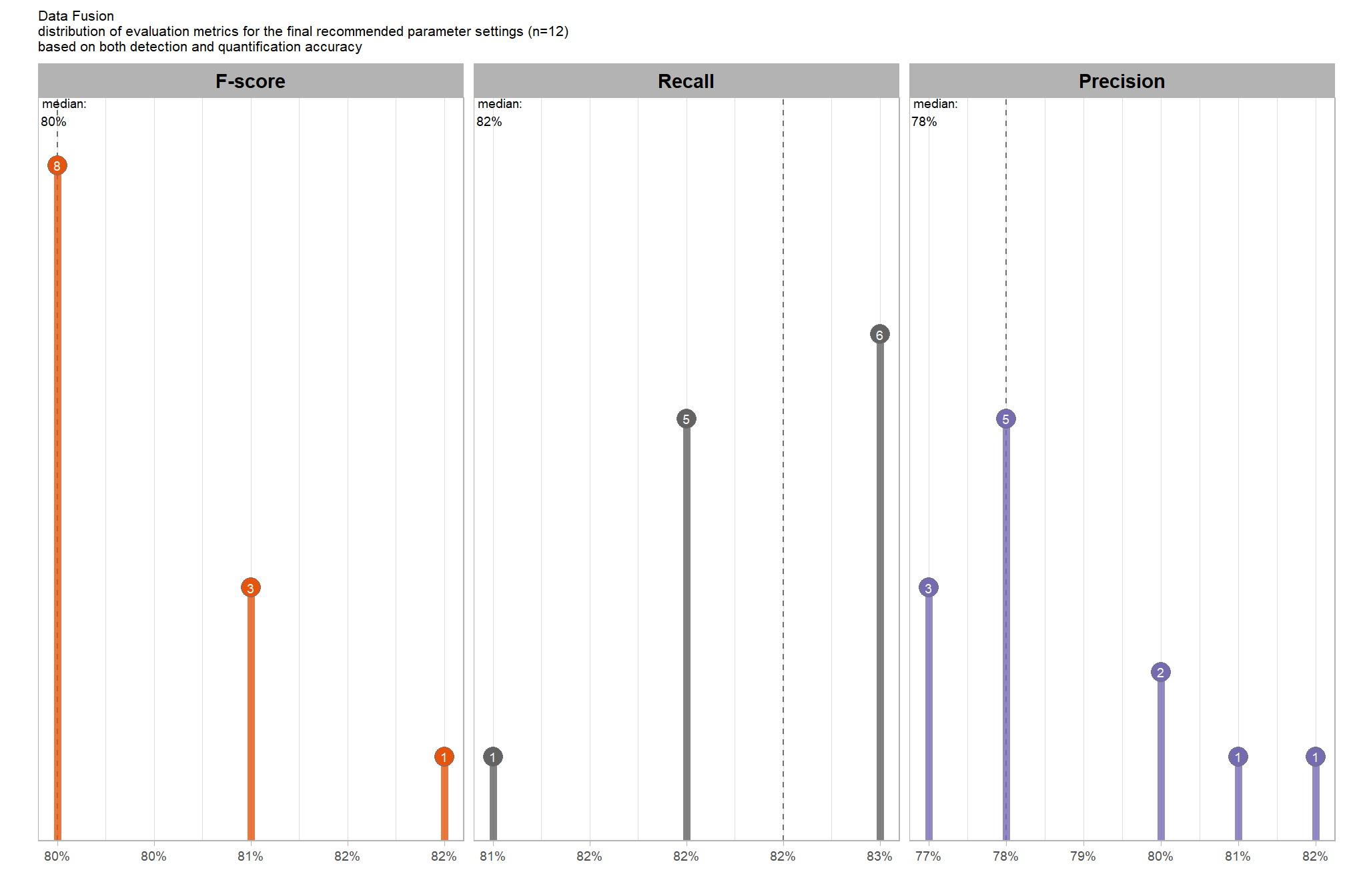
the primary takeaway from this plot is that coarser resolution CHM data produces significantly worse diameter quantification accuracy (i.e. higher MAPE) irrespective of the inclusion of spectral data or it’s weighting. if the objective is to quantify slash pile form with any sort of accuracy, a CHM resolution of 0.2m or finer is needed. based on the vertex of the parabola, the optimal CHM resolution for accurately quantifying diameter is between 0.1m and 0.2m. remember that the inclusion of spectral data in the data fusion detection methodology does not alter candidate pile form nor add new piles, so we don’t expect much variability in quantification accuracy at a given CHM resolution based on the inclusion of spectral data. any changes in overall pile quantification accuracy (e.g. when aggregated to the stand level) from the inclusion of spectral data is a result of the spectral data filtering out candidate piles that would otherwise alter the overall, aggregated accuracy.
we can look at the posterior distributions of the expected Diameter MAPE at different CHM resolution levels by the inclusion (or exclusion) of spectral data and it’s weighting
draws_temp %>%
ggplot2::ggplot(mapping = ggplot2::aes(y=value, x=chm_res_m)) +
tidybayes::stat_eye(
mapping = ggplot2::aes(fill = spectral_weight)
, point_interval = median_hdi, .width = .95
, slab_alpha = 0.95
, interval_color = "gray44", linewidth = 1
, point_color = "gray44", point_fill = "gray44", point_size = 1
) +
ggplot2::facet_grid(cols = dplyr::vars(spectral_weight), labeller = "label_both") +
ggplot2::scale_fill_manual(values = pal_spectral_weight) +
ggplot2::scale_y_continuous(labels = scales::percent, breaks = scales::breaks_extended(16)) +
ggplot2::labs(x = "CHM resolution", y = "Diameter MAPE") +
ggplot2::theme_light() +
ggplot2::theme(
legend.position = "none"
, strip.text = ggplot2::element_text(size = 8, color = "black", face = "bold")
)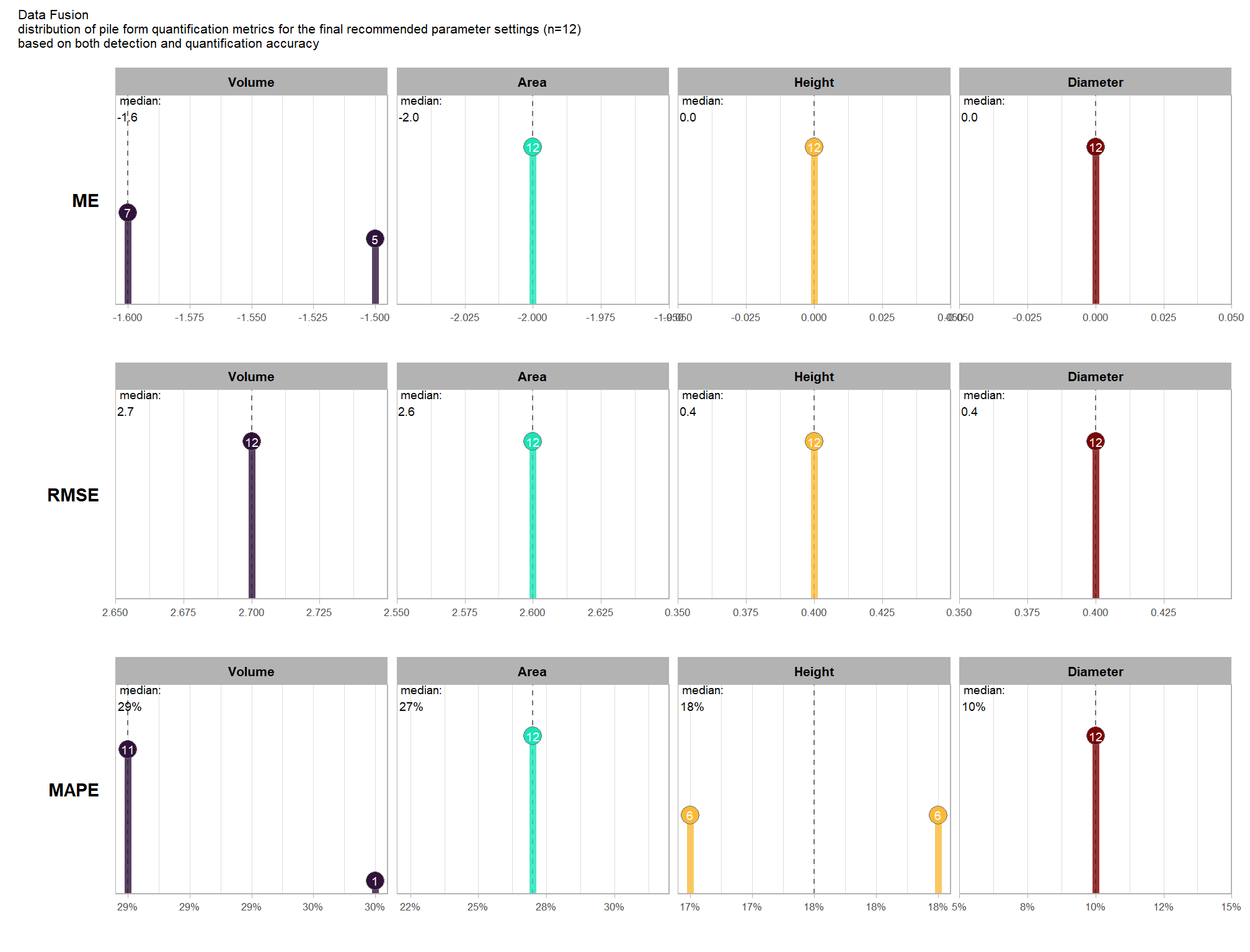
those are some tight posterior distributions and HDI’s, meaning our model is very confident in the expected diameter accuracy at the CHM resolutions tested. put another way, the output from our pile detection methodology is consistent in terms of quantification of detected pile diameter and it’s error relative to field-measured values.
table that
draws_temp %>%
dplyr::mutate(spectral_weight = forcats::fct_relabel(spectral_weight,~paste0("spectral_weight: ", .x, recycle0 = T))) %>%
dplyr::group_by(spectral_weight, chm_res_m) %>%
dplyr::summarise(
# get median_hdi
median_hdi_est = tidybayes::median_hdci(value)$y
, median_hdi_lower = tidybayes::median_hdci(value)$ymin
, median_hdi_upper = tidybayes::median_hdci(value)$ymax
) %>%
# format pcts
dplyr::mutate(dplyr::across(
tidyselect::starts_with("median_hdi_")
, ~ scales::percent(.x, accuracy = 0.1)
)) %>%
dplyr::ungroup() %>%
dplyr::arrange(spectral_weight, chm_res_m) %>%
kableExtra::kbl(
digits = 2
, caption = "Diameter MAPE<br>95% HDI of the posterior predictive distribution"
, col.names = c(
"spectral_weight", "CHM resolution"
, c("Diameter MAPE<br>median", "HDI low", "HDI high")
)
, escape = F
) %>%
kableExtra::kable_styling() %>%
kableExtra::collapse_rows(columns = 1, valign = "top") %>%
kableExtra::scroll_box(height = "8in")| spectral_weight | CHM resolution |
Diameter MAPE median |
HDI low | HDI high |
|---|---|---|---|---|
| spectral_weight: 0 | 0.1 | 10.9% | 10.8% | 11.1% |
| 0.2 | 18.1% | 17.9% | 18.3% | |
| 0.3 | 26.9% | 26.7% | 27.1% | |
| 0.4 | 35.9% | 35.6% | 36.2% | |
| 0.5 | 43.1% | 42.6% | 43.6% | |
| spectral_weight: 1 | 0.1 | 10.9% | 10.8% | 11.1% |
| 0.2 | 18.1% | 17.9% | 18.3% | |
| 0.3 | 26.9% | 26.7% | 27.1% | |
| 0.4 | 35.9% | 35.6% | 36.2% | |
| 0.5 | 43.1% | 42.6% | 43.6% | |
| spectral_weight: 2 | 0.1 | 10.9% | 10.8% | 11.1% |
| 0.2 | 18.1% | 17.9% | 18.3% | |
| 0.3 | 26.9% | 26.7% | 27.1% | |
| 0.4 | 35.9% | 35.6% | 36.2% | |
| 0.5 | 43.1% | 42.5% | 43.6% | |
| spectral_weight: 3 | 0.1 | 10.9% | 10.8% | 11.1% |
| 0.2 | 18.1% | 17.9% | 18.3% | |
| 0.3 | 26.9% | 26.7% | 27.2% | |
| 0.4 | 35.9% | 35.6% | 36.3% | |
| 0.5 | 43.1% | 42.6% | 43.6% | |
| spectral_weight: 4 | 0.1 | 10.9% | 10.8% | 11.1% |
| 0.2 | 18.1% | 17.9% | 18.3% | |
| 0.3 | 26.9% | 26.7% | 27.1% | |
| 0.4 | 35.9% | 35.6% | 36.3% | |
| 0.5 | 43.1% | 42.5% | 43.6% | |
| spectral_weight: 5 | 0.1 | 11.5% | 11.4% | 11.7% |
| 0.2 | 18.9% | 18.7% | 19.0% | |
| 0.3 | 27.8% | 27.5% | 28.0% | |
| 0.4 | 36.6% | 36.3% | 37.0% | |
| 0.5 | 43.4% | 42.9% | 44.0% |
now we’ll probabilistically test the hypothesis that coarser resolution CHM data results in lower diameter quantification accuracy and determine by how much. we’ll look at the influence of CHM resolution based on the inclusion of spectral data (or exclusion) and it’s weighting determined by the spectral_weight parameter
we’ll only make contrasts against the lowest CHM resolution tested which will be treated as a “control” in the tidybayes::compare_levels() call
contrast_temp <-
draws_temp %>%
dplyr::group_by(spectral_weight) %>%
tidybayes::compare_levels(
value
, by = chm_res_m
, comparison =
"control"
# tidybayes::emmeans_comparison("revpairwise")
# "pairwise"
) %>%
# dplyr::glimpse()
dplyr::rename(contrast = chm_res_m) %>%
# group the data before calculating contrast variables %>%
dplyr::group_by(spectral_weight, contrast) %>%
make_contrast_vars() %>%
# relabel the label for the facets
dplyr::mutate(spectral_weight = forcats::fct_relabel(spectral_weight,~paste0("spectral_weight: ", .x, recycle0 = T)))
# huh?
# contrast_temp %>% dplyr::glimpse()
# plot it
plt_contrast(
contrast_temp
# , caption_text = form_temp
, y_axis_title = "CHM resolution contrast"
, x_axis_title = "difference (Diameter MAPE)"
, facet = "spectral_weight"
, label_size = 2.5
, x_expand = c(0.1,0.6)
# , annotate_which = "right"
) +
labs(
subtitle = "posterior predictive distribution of group constrasts with 95% & 50% HDI\nby `spectral_weight`"
)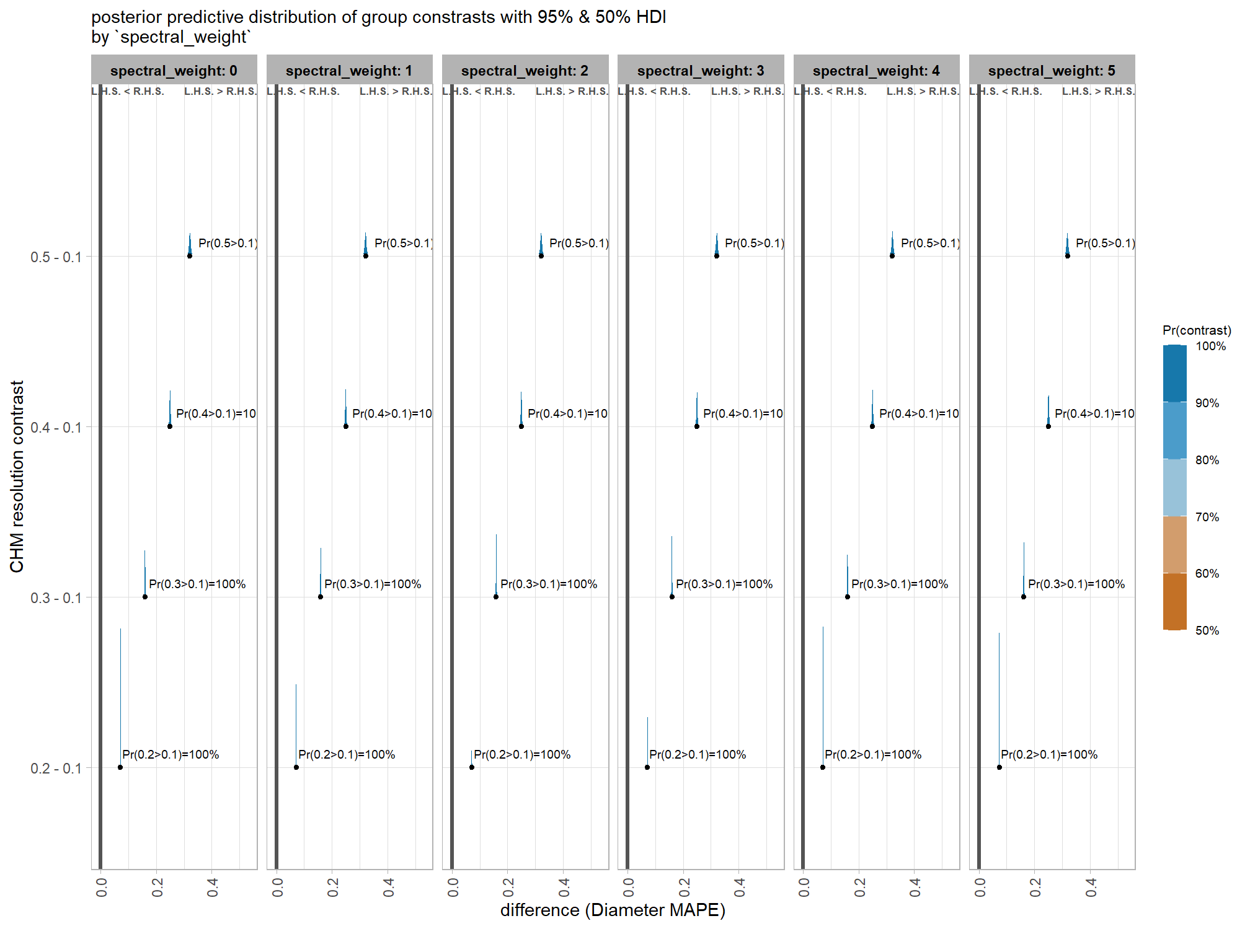
let’s table it
contrast_temp %>%
dplyr::distinct(
spectral_weight, contrast
, median_hdi_est, median_hdi_lower, median_hdi_upper
, pr_gt_zero # , pr_lt_zero
) %>%
# format pcts
dplyr::mutate(dplyr::across(
tidyselect::starts_with("median_hdi_")
, ~ scales::percent(.x, accuracy = 0.1)
)) %>%
dplyr::arrange(spectral_weight, contrast) %>%
kableExtra::kbl(
digits = 2
, caption = "brms::brm model: 95% HDI of the posterior predictive distribution of group constrasts"
, col.names = c(
"spectral_weight", "CHM res. contrast"
, "difference (Diameter MAPE)"
, "HDI low", "HDI high"
, "Pr(diff>0)"
)
, escape = F
) %>%
kableExtra::kable_styling() %>%
kableExtra::collapse_rows(columns = 1, valign = "top") %>%
kableExtra::scroll_box(height = "8in")| spectral_weight | CHM res. contrast | difference (Diameter MAPE) | HDI low | HDI high | Pr(diff>0) |
|---|---|---|---|---|---|
| spectral_weight: 0 | 0.2 - 0.1 | 7.2% | 7.1% | 7.3% | 100% |
| 0.3 - 0.1 | 16.0% | 15.8% | 16.2% | 100% | |
| 0.4 - 0.1 | 25.0% | 24.6% | 25.3% | 100% | |
| 0.5 - 0.1 | 32.1% | 31.6% | 32.7% | 100% | |
| spectral_weight: 1 | 0.2 - 0.1 | 7.2% | 7.1% | 7.3% | 100% |
| 0.3 - 0.1 | 16.0% | 15.8% | 16.2% | 100% | |
| 0.4 - 0.1 | 25.0% | 24.7% | 25.3% | 100% | |
| 0.5 - 0.1 | 32.2% | 31.6% | 32.8% | 100% | |
| spectral_weight: 2 | 0.2 - 0.1 | 7.2% | 7.1% | 7.3% | 100% |
| 0.3 - 0.1 | 16.0% | 15.8% | 16.2% | 100% | |
| 0.4 - 0.1 | 25.0% | 24.6% | 25.3% | 100% | |
| 0.5 - 0.1 | 32.1% | 31.5% | 32.6% | 100% | |
| spectral_weight: 3 | 0.2 - 0.1 | 7.2% | 7.1% | 7.2% | 100% |
| 0.3 - 0.1 | 16.0% | 15.8% | 16.2% | 100% | |
| 0.4 - 0.1 | 25.0% | 24.7% | 25.4% | 100% | |
| 0.5 - 0.1 | 32.2% | 31.6% | 32.7% | 100% | |
| spectral_weight: 4 | 0.2 - 0.1 | 7.2% | 7.1% | 7.3% | 100% |
| 0.3 - 0.1 | 16.0% | 15.8% | 16.2% | 100% | |
| 0.4 - 0.1 | 25.0% | 24.7% | 25.4% | 100% | |
| 0.5 - 0.1 | 32.2% | 31.6% | 32.7% | 100% | |
| spectral_weight: 5 | 0.2 - 0.1 | 7.3% | 7.3% | 7.4% | 100% |
| 0.3 - 0.1 | 16.2% | 16.0% | 16.4% | 100% | |
| 0.4 - 0.1 | 25.1% | 24.8% | 25.5% | 100% | |
| 0.5 - 0.1 | 31.9% | 31.3% | 32.5% | 100% |
it is clear from these contrasts that coarser CHM resolutions lead to a decrease in diameter quantification accuracy and the pattern and difference in accuracy between resolution levels is consistent whether or not spectral data is included and it’s weighting if included. taking the method that does not use spectral data as an example (i.e. spectral_weight = 0), the lowest diameter MAPE of 10.6% was achieved using a 0.1m CHM and the diameter quantification accuracy decreased (MAPE increased) steadily as CHM resolution became more coarse with a 41.8% diameter MAPE expected fore the 0.5 m resolution data. we can be certain (>99% probability) that there is a significant decrease in diameter quantification accuracy (i.e. increase in MAPE) for coarser resolution CHM data compared to finer resolution data.
9.2.5.2.2 Spectral data
now we’ll look at the impact of including (or excluding) spectral data and the weighting of the spectral_weight parameter where a value of “0” indicates no spectral data was used (i.e. structural only), the lowest weighting of the spectral data is “1” (only one spectral index threshold must be met), and the highest weighting of spectral data is “5” (all spectral index thresholds must be met).
Note: we expect that the spectral data does not significantly alter the quantification of slash pile form. this is because spectral information is used solely to filter candidate piles, meaning it neither reshapes existing ones nor introduces new detections.
# viridis::rocket(5, begin = 0.9, end = 0.6) %>% scales::show_col()
# brms::posterior_summary(brms_diam_mape_mod)
draws_temp %>%
dplyr::filter(
round(chm_res_m,2) == round(chm_res_m,1) # let's just look at every 0.1 m (10 cm)
) %>%
ggplot2::ggplot(mapping = ggplot2::aes(x = spectral_weight, y = value, color = factor(chm_res_m))) +
# tidybayes::stat_halfeye() +
tidybayes::stat_lineribbon(point_interval = "median_hdi", .width = c(0.95)) +
# ggplot2::facet_wrap(facets = dplyr::vars(spectral_weight))
ggplot2::scale_fill_brewer(palette = "Greys") +
ggplot2::scale_color_viridis_d(option = "rocket", begin = 0.9, end = 0.6) +
ggplot2::scale_y_continuous(labels = scales::percent) +
ggplot2::labs(x = "`spectral_weight`", color = "CHM resolution", y = "Diameter MAPE") +
ggplot2::theme_light() +
ggplot2::theme(
legend.position = "top"
) +
ggplot2::guides(
color = ggplot2::guide_legend(override.aes = list(shape = 15, lwd = 8, fill = NA))
, fill = "none"
)
while there is a slight decrease in diameter quantification accuracy (increase in MAPE) at the highest spectral weighting, the inclusion of spectral data and the setting of the spectral_weight parameter does not significantly alter the form quantification accuracy irrespective of the CHM resolution
we can look at the posterior distributions of the expected Diameter MAPE at different spectral_weight settings by the input CHM resolution
draws_temp %>%
dplyr::filter(
round(chm_res_m,2) == round(chm_res_m,1) # let's just look at every 0.1 m (10 cm)
) %>%
dplyr::mutate(chm_res_m = chm_res_m %>% factor() %>% forcats::fct_relabel(~paste0("CHM resolution: ", .x, recycle0 = T))) %>%
ggplot2::ggplot(mapping = ggplot2::aes(y=value, x=spectral_weight)) +
tidybayes::stat_eye(
mapping = ggplot2::aes(fill = chm_res_m)
, point_interval = median_hdi, .width = .95
, slab_alpha = 0.95
, interval_color = "gray44", linewidth = 1
, point_color = "gray44", point_fill = "gray44", point_size = 1
) +
ggplot2::facet_grid(cols = dplyr::vars(chm_res_m)) +
ggplot2::scale_fill_viridis_d(option = "rocket", begin = 0.9, end = 0.6) +
ggplot2::scale_y_continuous(limits = c(0,NA), labels = scales::percent, breaks = scales::breaks_extended(16)) +
ggplot2::labs(x = "`spectral_weight`", y = "Diameter MAPE") +
ggplot2::theme_light() +
ggplot2::theme(
legend.position = "none"
, strip.text = ggplot2::element_text(size = 8, color = "black", face = "bold")
)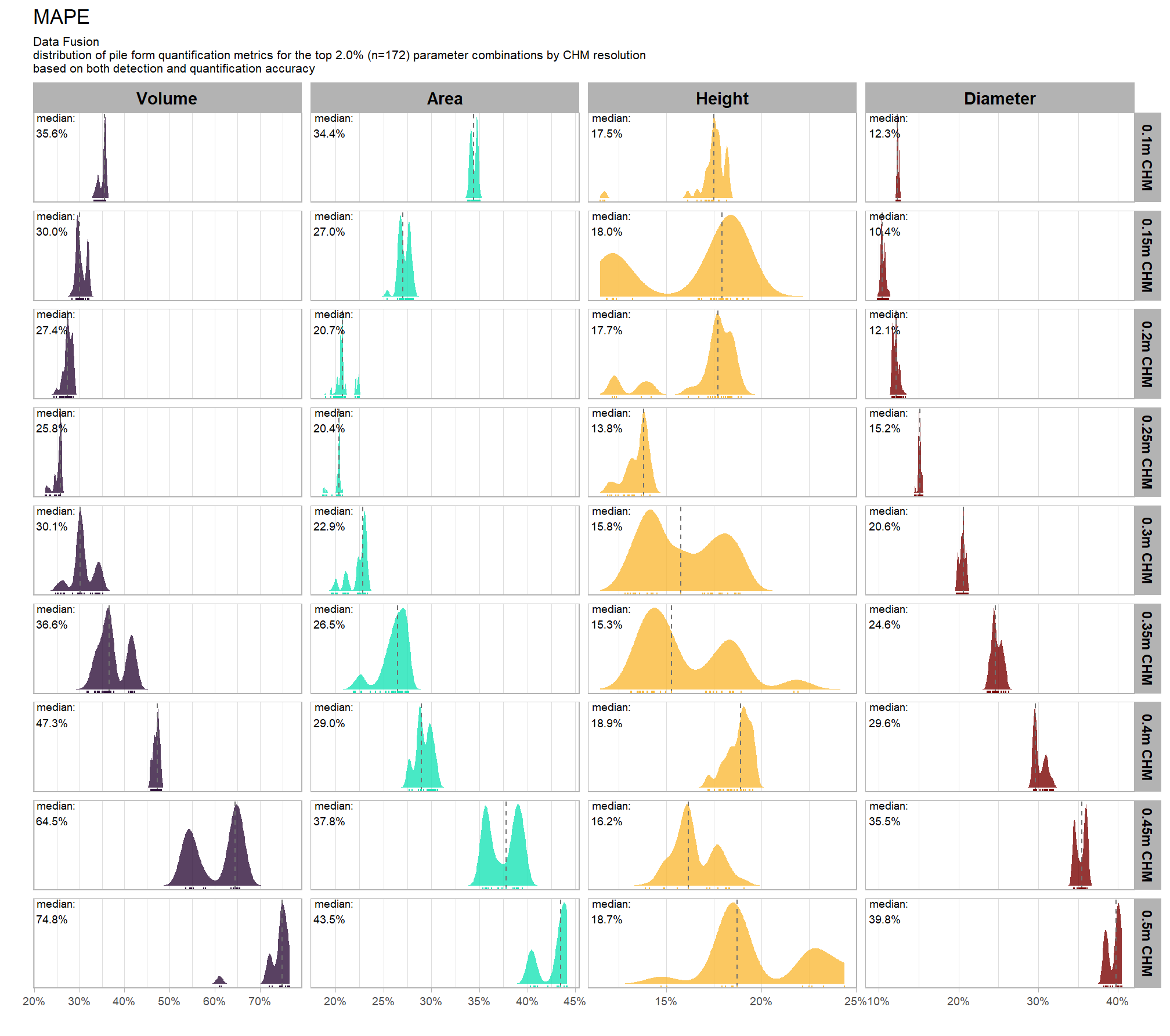
we already saw this same data above in our CHM resolution testing, but we’ll table that again but this time grouping by CHM resolution
draws_temp %>%
dplyr::filter(
round(chm_res_m,2) == round(chm_res_m,1) # let's just look at every 0.1 m (10 cm)
) %>%
dplyr::mutate(chm_res_m = chm_res_m %>% factor() %>% forcats::fct_relabel(~paste0("CHM resolution: ", .x, recycle0 = T))) %>%
dplyr::group_by(chm_res_m, spectral_weight) %>%
dplyr::summarise(
# get median_hdi
median_hdi_est = tidybayes::median_hdci(value)$y
, median_hdi_lower = tidybayes::median_hdci(value)$ymin
, median_hdi_upper = tidybayes::median_hdci(value)$ymax
) %>%
# format pcts
dplyr::mutate(dplyr::across(
tidyselect::starts_with("median_hdi_")
, ~ scales::percent(.x, accuracy = 0.1)
)) %>%
dplyr::ungroup() %>%
dplyr::arrange(chm_res_m,spectral_weight) %>%
kableExtra::kbl(
digits = 2
, caption = "Diameter MAPE<br>95% HDI of the posterior predictive distribution"
, col.names = c(
"CHM resolution", "spectral_weight"
, c("Diameter MAPE<br>median", "HDI low", "HDI high")
)
, escape = F
) %>%
kableExtra::kable_styling() %>%
kableExtra::collapse_rows(columns = 1, valign = "top") %>%
kableExtra::scroll_box(height = "8in")| CHM resolution | spectral_weight |
Diameter MAPE median |
HDI low | HDI high |
|---|---|---|---|---|
| CHM resolution: 0.1 | 0 | 10.9% | 10.8% | 11.1% |
| 1 | 10.9% | 10.8% | 11.1% | |
| 2 | 10.9% | 10.8% | 11.1% | |
| 3 | 10.9% | 10.8% | 11.1% | |
| 4 | 10.9% | 10.8% | 11.1% | |
| 5 | 11.5% | 11.4% | 11.7% | |
| CHM resolution: 0.2 | 0 | 18.1% | 17.9% | 18.3% |
| 1 | 18.1% | 17.9% | 18.3% | |
| 2 | 18.1% | 17.9% | 18.3% | |
| 3 | 18.1% | 17.9% | 18.3% | |
| 4 | 18.1% | 17.9% | 18.3% | |
| 5 | 18.9% | 18.7% | 19.0% | |
| CHM resolution: 0.3 | 0 | 26.9% | 26.7% | 27.1% |
| 1 | 26.9% | 26.7% | 27.1% | |
| 2 | 26.9% | 26.7% | 27.1% | |
| 3 | 26.9% | 26.7% | 27.2% | |
| 4 | 26.9% | 26.7% | 27.1% | |
| 5 | 27.8% | 27.5% | 28.0% | |
| CHM resolution: 0.4 | 0 | 35.9% | 35.6% | 36.2% |
| 1 | 35.9% | 35.6% | 36.2% | |
| 2 | 35.9% | 35.6% | 36.2% | |
| 3 | 35.9% | 35.6% | 36.3% | |
| 4 | 35.9% | 35.6% | 36.3% | |
| 5 | 36.6% | 36.3% | 37.0% | |
| CHM resolution: 0.5 | 0 | 43.1% | 42.6% | 43.6% |
| 1 | 43.1% | 42.6% | 43.6% | |
| 2 | 43.1% | 42.5% | 43.6% | |
| 3 | 43.1% | 42.6% | 43.6% | |
| 4 | 43.1% | 42.5% | 43.6% | |
| 5 | 43.4% | 42.9% | 44.0% |
now we’ll probabilistically test the hypothesis that the inclusion of spectral data improves detection accuracy and quantify by how much. we’ll look at the influence of spectral data based on the CHM resolution
to actually compare the different levels of spectral_weight, we’ll use the MCMC draws to contrast the posterior predictions at different levels of the parameter (see below)
contrast_temp <-
draws_temp %>%
dplyr::filter(
round(chm_res_m,2) == round(chm_res_m,1) # let's just look at every 0.1 m (10 cm)
) %>%
dplyr::group_by(chm_res_m) %>%
tidybayes::compare_levels(
value
, by = spectral_weight
, comparison =
# tidybayes::emmeans_comparison("revpairwise")
"pairwise"
) %>%
# dplyr::glimpse()
dplyr::rename(contrast = spectral_weight) %>%
# group the data before calculating contrast variables %>%
dplyr::group_by(chm_res_m, contrast) %>%
make_contrast_vars() %>%
# relabel the label for the facets
dplyr::mutate(chm_res_m = chm_res_m %>% factor() %>% forcats::fct_relabel(~paste0("CHM resolution: ", .x, recycle0 = T)))
# huh?
# contrast_temp %>% dplyr::glimpse()
# plot it
plt_contrast(
contrast_temp
# , caption_text = form_temp
, y_axis_title = "`spectral_weight` contrast"
, x_axis_title = "difference (Diameter MAPE)"
, facet = "chm_res_m"
, label_size = 2
, x_expand = c(0.5,0.5)
) +
labs(
subtitle = "posterior predictive distribution of group constrasts with 95% & 50% HDI\nby `chm_res_m`"
)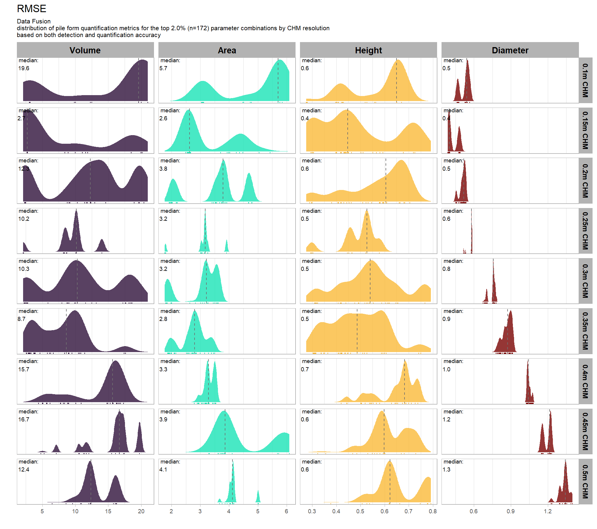
let’s table it
contrast_temp %>%
dplyr::distinct(
chm_res_m, contrast
, median_hdi_est, median_hdi_lower, median_hdi_upper
# , pr_lt_zero
, pr_gt_zero
) %>%
dplyr::arrange(chm_res_m, contrast) %>%
# format pcts
dplyr::mutate(dplyr::across(
tidyselect::starts_with("median_hdi_")
, ~ scales::percent(.x, accuracy = 0.1)
)) %>%
kableExtra::kbl(
digits = 2
, caption = "brms::brm model: 95% HDI of the posterior predictive distribution of group constrasts"
, col.names = c(
"CHM resolution", "spectral_weight"
, "difference (Diameter MAPE)"
, "HDI low", "HDI high"
# , "Pr(diff<0)"
, "Pr(diff>0)"
)
, escape = F
) %>%
kableExtra::kable_styling() %>%
kableExtra::collapse_rows(columns = 1, valign = "top") %>%
kableExtra::scroll_box(height = "8in")| CHM resolution | spectral_weight | difference (Diameter MAPE) | HDI low | HDI high | Pr(diff>0) |
|---|---|---|---|---|---|
| CHM resolution: 0.1 | 1 - 0 | 0.0% | -0.2% | 0.2% | 47% |
| 2 - 0 | 0.0% | -0.2% | 0.2% | 50% | |
| 2 - 1 | 0.0% | -0.2% | 0.2% | 53% | |
| 3 - 0 | 0.0% | -0.2% | 0.2% | 49% | |
| 3 - 1 | 0.0% | -0.2% | 0.2% | 50% | |
| 3 - 2 | 0.0% | -0.2% | 0.2% | 50% | |
| 4 - 0 | 0.0% | -0.2% | 0.2% | 48% | |
| 4 - 1 | 0.0% | -0.2% | 0.2% | 51% | |
| 4 - 2 | 0.0% | -0.2% | 0.2% | 50% | |
| 4 - 3 | 0.0% | -0.2% | 0.2% | 51% | |
| 5 - 0 | 0.6% | 0.4% | 0.8% | 100% | |
| 5 - 1 | 0.6% | 0.4% | 0.8% | 100% | |
| 5 - 2 | 0.6% | 0.4% | 0.8% | 100% | |
| 5 - 3 | 0.6% | 0.4% | 0.8% | 100% | |
| 5 - 4 | 0.6% | 0.4% | 0.8% | 100% | |
| CHM resolution: 0.2 | 1 - 0 | 0.0% | -0.2% | 0.2% | 48% |
| 2 - 0 | 0.0% | -0.2% | 0.2% | 48% | |
| 2 - 1 | 0.0% | -0.2% | 0.2% | 53% | |
| 3 - 0 | 0.0% | -0.2% | 0.2% | 49% | |
| 3 - 1 | 0.0% | -0.2% | 0.2% | 49% | |
| 3 - 2 | 0.0% | -0.2% | 0.2% | 51% | |
| 4 - 0 | 0.0% | -0.2% | 0.2% | 50% | |
| 4 - 1 | 0.0% | -0.2% | 0.2% | 50% | |
| 4 - 2 | 0.0% | -0.2% | 0.2% | 49% | |
| 4 - 3 | 0.0% | -0.2% | 0.2% | 51% | |
| 5 - 0 | 0.8% | 0.6% | 1.0% | 100% | |
| 5 - 1 | 0.8% | 0.6% | 1.0% | 100% | |
| 5 - 2 | 0.8% | 0.6% | 1.0% | 100% | |
| 5 - 3 | 0.8% | 0.6% | 1.0% | 100% | |
| 5 - 4 | 0.8% | 0.6% | 1.0% | 100% | |
| CHM resolution: 0.3 | 1 - 0 | 0.0% | -0.2% | 0.3% | 49% |
| 2 - 0 | 0.0% | -0.2% | 0.3% | 47% | |
| 2 - 1 | 0.0% | -0.2% | 0.2% | 50% | |
| 3 - 0 | 0.0% | -0.2% | 0.3% | 48% | |
| 3 - 1 | 0.0% | -0.2% | 0.3% | 51% | |
| 3 - 2 | 0.0% | -0.2% | 0.2% | 51% | |
| 4 - 0 | 0.0% | -0.2% | 0.3% | 49% | |
| 4 - 1 | 0.0% | -0.2% | 0.3% | 50% | |
| 4 - 2 | 0.0% | -0.2% | 0.2% | 51% | |
| 4 - 3 | 0.0% | -0.2% | 0.2% | 51% | |
| 5 - 0 | 0.8% | 0.6% | 1.1% | 100% | |
| 5 - 1 | 0.9% | 0.6% | 1.1% | 100% | |
| 5 - 2 | 0.9% | 0.6% | 1.1% | 100% | |
| 5 - 3 | 0.9% | 0.6% | 1.1% | 100% | |
| 5 - 4 | 0.8% | 0.6% | 1.1% | 100% | |
| CHM resolution: 0.4 | 1 - 0 | 0.0% | -0.4% | 0.4% | 50% |
| 2 - 0 | 0.0% | -0.4% | 0.4% | 49% | |
| 2 - 1 | 0.0% | -0.4% | 0.4% | 49% | |
| 3 - 0 | 0.0% | -0.4% | 0.3% | 49% | |
| 3 - 1 | 0.0% | -0.4% | 0.4% | 51% | |
| 3 - 2 | 0.0% | -0.4% | 0.4% | 54% | |
| 4 - 0 | 0.0% | -0.4% | 0.4% | 51% | |
| 4 - 1 | 0.0% | -0.4% | 0.4% | 50% | |
| 4 - 2 | 0.0% | -0.3% | 0.4% | 52% | |
| 4 - 3 | 0.0% | -0.4% | 0.4% | 51% | |
| 5 - 0 | 0.7% | 0.3% | 1.1% | 100% | |
| 5 - 1 | 0.7% | 0.3% | 1.1% | 100% | |
| 5 - 2 | 0.7% | 0.3% | 1.1% | 100% | |
| 5 - 3 | 0.7% | 0.3% | 1.1% | 100% | |
| 5 - 4 | 0.7% | 0.3% | 1.1% | 100% | |
| CHM resolution: 0.5 | 1 - 0 | 0.0% | -0.6% | 0.7% | 50% |
| 2 - 0 | 0.0% | -0.6% | 0.7% | 51% | |
| 2 - 1 | 0.0% | -0.7% | 0.7% | 48% | |
| 3 - 0 | 0.0% | -0.7% | 0.6% | 51% | |
| 3 - 1 | 0.0% | -0.6% | 0.7% | 50% | |
| 3 - 2 | 0.0% | -0.6% | 0.6% | 52% | |
| 4 - 0 | 0.0% | -0.7% | 0.7% | 53% | |
| 4 - 1 | 0.0% | -0.6% | 0.8% | 51% | |
| 4 - 2 | 0.0% | -0.6% | 0.7% | 51% | |
| 4 - 3 | 0.0% | -0.6% | 0.7% | 49% | |
| 5 - 0 | 0.4% | -0.3% | 1.0% | 85% | |
| 5 - 1 | 0.3% | -0.3% | 1.1% | 84% | |
| 5 - 2 | 0.4% | -0.3% | 1.1% | 86% | |
| 5 - 3 | 0.4% | -0.4% | 1.0% | 86% | |
| 5 - 4 | 0.4% | -0.3% | 1.0% | 84% |
although we can be very certain that there are differences in diameter quantification accuracy (>99% probability across most CHM resolutions) when the spectral_weight is set to “5” (i.e. requiring that all spectral criteria be met) compared to the other settings of spectral_weight or not including spectral data, these differences are so small with nearly all of them showing a difference in diameter MAPE of <1%.
9.3 Bayesian GLM - Height MAPE
9.3.1 Model selection
we’re going to use a sub-sample of the data to perform model testing. our objective is to construct the model such that it faithfully represents the data.
we reviewed the main effect parameter trends against MAPE here and used these to guide our model design. we’ll follow Kurz 2025 and compare our models with the LOO information criterion
Like other information criteria, the LOO values aren’t of interest in and of themselves. However, the values of one model’s LOO relative to that of another is of great interest. We generally prefer models with lower estimates.
# subsample data
set.seed(222)
ms_df_temp <- param_combos_spectral_ranked %>% dplyr::slice_sample(prop = 0.11)
# mcmc setup
iter_temp <- 2444
warmup_temp <- 1222
chains_temp <- 4
####################################################################
# base model with form selected based on main effect trends
####################################################################
height_mape_mod1_temp <- brms::brm(
formula = pct_diff_height_m_mape ~
0 + # no intercept to allow all values of spectral_weight to be shown instead of set as the baseline
max_ht_m + max_area_m2 + convexity_pct + circle_fit_iou_pct +
chm_res_m +
spectral_weight + chm_res_m:spectral_weight
, data = ms_df_temp
, family = Gamma(link = "log")
# mcmc
, iter = iter_temp, warmup = warmup_temp
, chains = chains_temp
# , control = list(adapt_delta = 0.999, max_treedepth = 13)
, cores = lasR::half_cores()
, file = paste0("../data/", "height_mape_mod1_temp")
)
height_mape_mod1_temp <- brms::add_criterion(height_mape_mod1_temp, criterion = "loo")
####################################################################
# allows slope and curvature of circle_fit_iou_pct to vary by chm_res_m and vice-versa
####################################################################
height_mape_mod2_temp <- brms::brm(
formula = pct_diff_height_m_mape ~
0 + # no intercept to allow all values of spectral_weight to be shown instead of set as the baseline
max_ht_m + max_area_m2 + convexity_pct +
circle_fit_iou_pct + I(circle_fit_iou_pct^2) + # changed from base model
chm_res_m +
spectral_weight + chm_res_m:spectral_weight
, data = ms_df_temp
, family = Gamma(link = "log")
# mcmc
, iter = iter_temp, warmup = warmup_temp
, chains = chains_temp
# , control = list(adapt_delta = 0.999, max_treedepth = 13)
, cores = lasR::half_cores()
, file = paste0("../data/", "height_mape_mod2_temp")
)
height_mape_mod2_temp <- brms::add_criterion(height_mape_mod2_temp, criterion = "loo")
####################################################################
# allows slope and curvature of circle_fit_iou_pct to vary by convexity_pct and vice-versa
####################################################################
height_mape_mod3_temp <- brms::brm(
formula = pct_diff_height_m_mape ~
0 + # no intercept to allow all values of spectral_weight to be shown instead of set as the baseline
max_ht_m + max_area_m2 +
convexity_pct + I(convexity_pct^2) + # changed from base model
circle_fit_iou_pct + I(circle_fit_iou_pct^2) + # changed from base model
convexity_pct:circle_fit_iou_pct + # changed from base model
chm_res_m +
spectral_weight + chm_res_m:spectral_weight
, data = ms_df_temp
, family = Gamma(link = "log")
# mcmc
, iter = iter_temp, warmup = warmup_temp
, chains = chains_temp
# , control = list(adapt_delta = 0.999, max_treedepth = 13)
, cores = lasR::half_cores()
, file = paste0("../data/", "height_mape_mod3_temp")
)
height_mape_mod3_temp <- brms::add_criterion(height_mape_mod3_temp, criterion = "loo")
####################################################################
# a three-way interaction of circle_fit_iou_pct, convexity_pct and chm_res_m
####################################################################
height_mape_mod4_temp <- brms::brm(
formula = pct_diff_height_m_mape ~
0 + # no intercept to allow all values of spectral_weight to be shown instead of set as the baseline
max_ht_m + max_area_m2 +
convexity_pct + I(convexity_pct^2) + # changed from base model
circle_fit_iou_pct + I(circle_fit_iou_pct^2) + # changed from base model
convexity_pct:circle_fit_iou_pct + # changed from base model
chm_res_m + I(chm_res_m^2) + # changed from base model
spectral_weight + chm_res_m:spectral_weight
, data = ms_df_temp
, family = Gamma(link = "log")
# mcmc
, iter = iter_temp, warmup = warmup_temp
, chains = chains_temp
# , control = list(adapt_delta = 0.999, max_treedepth = 13)
, cores = lasR::half_cores()
, file = paste0("../data/", "height_mape_mod4_temp")
)
height_mape_mod4_temp <- brms::add_criterion(height_mape_mod4_temp, criterion = "loo")
####################################################################
# a three-way interaction of circle_fit_iou_pct, convexity_pct and chm_res_m
####################################################################
height_mape_mod5_temp <- brms::brm(
formula = pct_diff_height_m_mape ~
0 + # no intercept to allow all values of spectral_weight to be shown instead of set as the baseline
max_ht_m + max_area_m2 +
convexity_pct + I(convexity_pct^2) + # changed from base model
circle_fit_iou_pct + I(circle_fit_iou_pct^2) + # changed from base model
convexity_pct:circle_fit_iou_pct + # changed from base model
convexity_pct:chm_res_m + # changed from base model
circle_fit_iou_pct:chm_res_m + # changed from base model
convexity_pct:circle_fit_iou_pct:chm_res_m + # changed from base model
chm_res_m +
spectral_weight + chm_res_m:spectral_weight
, data = ms_df_temp
, family = Gamma(link = "log")
# mcmc
, iter = iter_temp, warmup = warmup_temp
, chains = chains_temp
# , control = list(adapt_delta = 0.999, max_treedepth = 13)
, cores = lasR::half_cores()
, file = paste0("../data/", "height_mape_mod5_temp")
)
height_mape_mod5_temp <- brms::add_criterion(height_mape_mod5_temp, criterion = "loo")
####################################################################
# a three-way interaction of circle_fit_iou_pct, convexity_pct and chm_res_m
####################################################################
height_mape_mod6_temp <- brms::brm(
formula = pct_diff_height_m_mape ~
0 + # no intercept to allow all values of spectral_weight to be shown instead of set as the baseline
max_ht_m + max_area_m2 +
convexity_pct + I(convexity_pct^2) + # changed from base model
circle_fit_iou_pct + I(circle_fit_iou_pct^2) + # changed from base model
convexity_pct:circle_fit_iou_pct + # changed from base model
convexity_pct:chm_res_m + # changed from base model
circle_fit_iou_pct:chm_res_m + # changed from base model
convexity_pct:circle_fit_iou_pct:chm_res_m + # changed from base model
chm_res_m + I(chm_res_m^2) + # changed from base model
spectral_weight + chm_res_m:spectral_weight
, data = ms_df_temp
, family = Gamma(link = "log")
# mcmc
, iter = iter_temp, warmup = warmup_temp
, chains = chains_temp
# , control = list(adapt_delta = 0.999, max_treedepth = 13)
, cores = lasR::half_cores()
, file = paste0("../data/", "height_mape_mod6_temp")
)
height_mape_mod6_temp <- brms::add_criterion(height_mape_mod6_temp, criterion = "loo")compare our models with the LOO information criterion. with the brms::loo_compare() function, we can compute a formal difference score between models with the output rank ordering the models such that the best fitting model appears on top. all models also receive a difference score relative to the best model and a standard error of the difference score
brms::loo_compare(
height_mape_mod1_temp, height_mape_mod2_temp, height_mape_mod3_temp
, height_mape_mod4_temp, height_mape_mod5_temp, height_mape_mod6_temp
) %>%
kableExtra::kbl(caption = "Height MAPE model selection with LOO information criterion") %>%
kableExtra::kable_styling()| elpd_diff | se_diff | elpd_loo | se_elpd_loo | p_loo | se_p_loo | looic | se_looic | |
|---|---|---|---|---|---|---|---|---|
| height_mape_mod6_temp | 0.0000 | 0.00000 | 6288.058 | 113.9030 | 44.88877 | 5.472842 | -12576.12 | 227.8060 |
| height_mape_mod5_temp | -128.8016 | 11.38928 | 6159.256 | 118.7742 | 45.39308 | 5.826347 | -12318.51 | 237.5484 |
| height_mape_mod4_temp | -240.8235 | 31.72005 | 6047.234 | 128.6006 | 46.03526 | 6.017574 | -12094.47 | 257.2011 |
| height_mape_mod3_temp | -343.5301 | 34.92927 | 5944.528 | 133.4217 | 45.74430 | 6.183430 | -11889.06 | 266.8435 |
| height_mape_mod2_temp | -345.5319 | 37.53070 | 5942.526 | 134.4929 | 40.24100 | 5.598372 | -11885.05 | 268.9857 |
| height_mape_mod1_temp | -368.9222 | 44.36319 | 5919.136 | 140.7629 | 40.86776 | 5.809111 | -11838.27 | 281.5258 |
we can also look at the AIC-type model weights
brms::model_weights(
height_mape_mod1_temp, height_mape_mod2_temp, height_mape_mod3_temp
, height_mape_mod4_temp, height_mape_mod5_temp, height_mape_mod6_temp
) %>%
round(digits = 4)we can also quickly look at the Bayeisan \(R^2\) returned from the brms::bayes_R2() function
dplyr::bind_rows(
brms::bayes_R2(height_mape_mod1_temp,summary=F) %>% dplyr::as_tibble() %>% dplyr::mutate(mod = "height_mape_mod1_temp")
, brms::bayes_R2(height_mape_mod2_temp,summary=F) %>% dplyr::as_tibble() %>% dplyr::mutate(mod = "height_mape_mod2_temp")
, brms::bayes_R2(height_mape_mod3_temp,summary=F) %>% dplyr::as_tibble() %>% dplyr::mutate(mod = "height_mape_mod3_temp")
, brms::bayes_R2(height_mape_mod4_temp,summary=F) %>% dplyr::as_tibble() %>% dplyr::mutate(mod = "height_mape_mod4_temp")
, brms::bayes_R2(height_mape_mod5_temp,summary=F) %>% dplyr::as_tibble() %>% dplyr::mutate(mod = "height_mape_mod5_temp")
, brms::bayes_R2(height_mape_mod6_temp,summary=F) %>% dplyr::as_tibble() %>% dplyr::mutate(mod = "height_mape_mod6_temp")
) %>%
dplyr::mutate(mod = factor(mod)) %>%
ggplot2::ggplot(mapping=ggplot2::aes(y=R2, x = mod)) +
tidybayes::stat_eye(
point_interval = median_hdi, .width = .95
, slab_alpha = 0.95
) +
# ggplot2::facet_grid(cols = dplyr::vars(spectral_weight)) +
# ggplot2::scale_fill_manual(values = pal_chm_res_m) +
ggplot2::labs(x = "", y = "Bayesian R-squared") +
ggplot2::theme_light()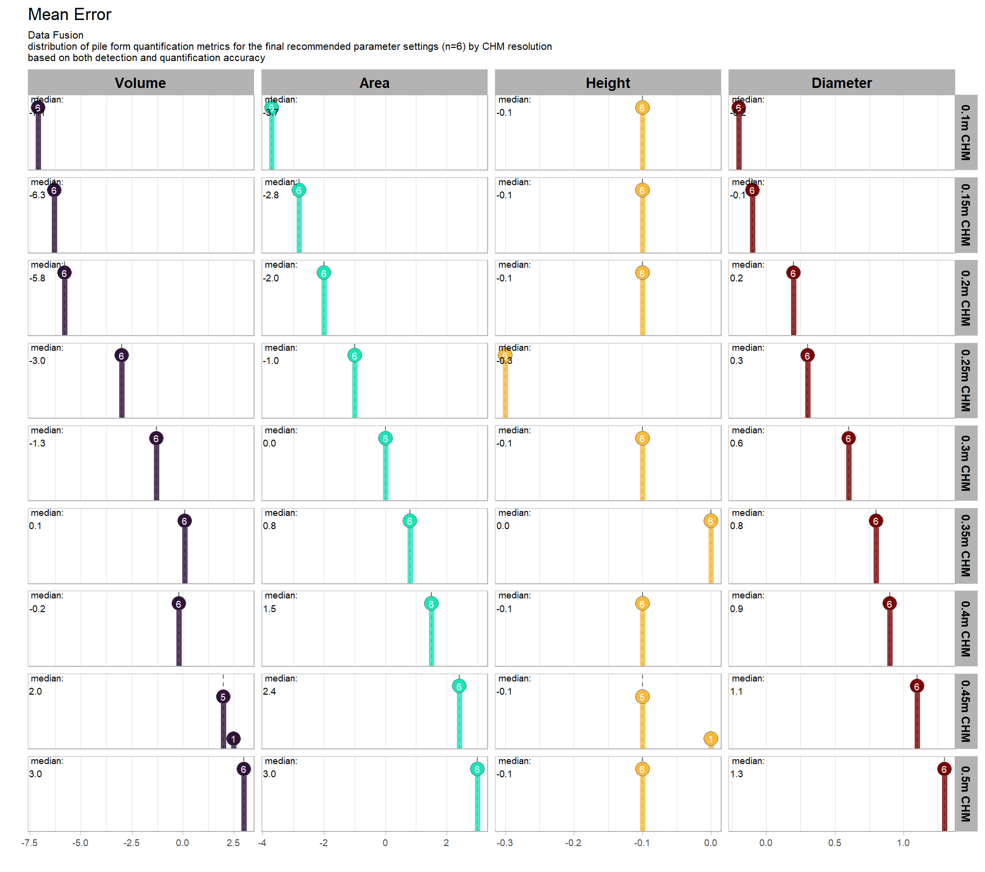
the more complex models were selected as the best. because the selected model includes quadratic terms and multiple interactions parameter interpretation will be a challenge, so we will have to rely on plotting the modeled relationships rather than trying to interpret the coefficients.
9.3.2 Modeling
the fully factored Bayesian statistical model that details the likelihood, linear model, and priors used is the same as above for Diameter MAPE
we reviewed the main effect parameter trends against MAPE here and used these to guide our model design
brms_height_mape_mod <- brms::brm(
formula = pct_diff_height_m_mape ~
0 + # no intercept to allow all values of spectral_weight to be shown instead of set as the baseline
max_ht_m + max_area_m2 +
convexity_pct + I(convexity_pct^2) + # changed from base model
circle_fit_iou_pct + I(circle_fit_iou_pct^2) + # changed from base model
convexity_pct:circle_fit_iou_pct + # changed from base model
convexity_pct:chm_res_m + # changed from base model
circle_fit_iou_pct:chm_res_m + # changed from base model
convexity_pct:circle_fit_iou_pct:chm_res_m + # changed from base model
chm_res_m + I(chm_res_m^2) + # changed from base model
spectral_weight + chm_res_m:spectral_weight
, data = param_combos_spectral_ranked # %>% dplyr::slice_sample(prop = 0.33)
, family = Gamma(link = "log")
# mcmc
, iter = 14000, warmup = 7000
, chains = 4
# , control = list(adapt_delta = 0.999, max_treedepth = 13)
, cores = lasR::half_cores()
, file = paste0("../data/", "brms_height_mape_mod")
)
# brms::make_stancode(brms_height_mape_mod)
# brms::prior_summary(brms_height_mape_mod)
# print(brms_height_mape_mod)
# brms::neff_ratio(brms_height_mape_mod)
# brms::rhat(brms_height_mape_mod)
# brms::nuts_params(brms_height_mape_mod)The brms::brm model summary
brms_height_mape_mod %>%
brms::posterior_summary() %>%
as.data.frame() %>%
tibble::rownames_to_column(var = "parameter") %>%
dplyr::rename_with(tolower) %>%
dplyr::filter(
stringr::str_starts(parameter, "b_")
| parameter == "phi"
) %>%
kableExtra::kbl(digits = 3, caption = "Bayesian model for Height MAPE") %>%
kableExtra::kable_styling()| parameter | estimate | est.error | q2.5 | q97.5 |
|---|---|---|---|---|
| b_max_ht_m | 0.075 | 0.001 | 0.073 | 0.077 |
| b_max_area_m2 | 0.002 | 0.000 | 0.002 | 0.002 |
| b_convexity_pct | 0.241 | 0.022 | 0.199 | 0.284 |
| b_Iconvexity_pctE2 | 0.016 | 0.014 | -0.012 | 0.043 |
| b_circle_fit_iou_pct | -0.750 | 0.025 | -0.799 | -0.701 |
| b_Icircle_fit_iou_pctE2 | 0.333 | 0.019 | 0.295 | 0.370 |
| b_chm_res_m | -1.839 | 0.050 | -1.938 | -1.741 |
| b_Ichm_res_mE2 | 3.247 | 0.065 | 3.119 | 3.375 |
| b_spectral_weight0 | -1.793 | 0.013 | -1.818 | -1.768 |
| b_spectral_weight1 | -1.793 | 0.013 | -1.818 | -1.768 |
| b_spectral_weight2 | -1.793 | 0.013 | -1.818 | -1.768 |
| b_spectral_weight3 | -1.793 | 0.013 | -1.818 | -1.768 |
| b_spectral_weight4 | -1.793 | 0.013 | -1.818 | -1.768 |
| b_spectral_weight5 | -1.817 | 0.013 | -1.842 | -1.792 |
| b_convexity_pct:circle_fit_iou_pct | 0.000 | 0.036 | -0.070 | 0.069 |
| b_convexity_pct:chm_res_m | -0.788 | 0.052 | -0.892 | -0.685 |
| b_circle_fit_iou_pct:chm_res_m | 1.790 | 0.057 | 1.678 | 1.903 |
| b_chm_res_m:spectral_weight1 | 0.000 | 0.026 | -0.051 | 0.051 |
| b_chm_res_m:spectral_weight2 | 0.000 | 0.026 | -0.053 | 0.051 |
| b_chm_res_m:spectral_weight3 | 0.000 | 0.026 | -0.052 | 0.051 |
| b_chm_res_m:spectral_weight4 | 0.000 | 0.027 | -0.052 | 0.052 |
| b_chm_res_m:spectral_weight5 | 0.057 | 0.026 | 0.006 | 0.110 |
| b_convexity_pct:circle_fit_iou_pct:chm_res_m | -0.199 | 0.106 | -0.407 | 0.008 |
note the quadratic coefficients ending in E2, Kruschke (2015) provides some insight on how to interpret:
A quadratic has the form \(y = \beta_{0} + \beta_{1}x + \beta_{2}x^{2}\). When \(\beta_{2}\) is zero, the form reduces to a line. Therefore, this extended model can produce any fit that the linear model can. When \(\beta_{2}\) is positive, a plot of the curve is a parabola that opens upward. When \(\beta_{2}\) is negative, the curve is a parabola that opens downward. We have no reason to think that the curvature in the family-income data is exactly a parabola, but the quadratic trend might describe the data much better than a line alone. (p. 496)
9.3.3 Posterior Predictive Checks
Markov chain Monte Carlo (MCMC) simulations were conducted using the brms package (Bürkner 2017) to estimate posterior predictive distributions of the parameters of interest. We ran 4 chains of 10,000 iterations with the first 5,000 discarded as burn-in. Trace-plots were utilized to visually assess model convergence.
check the trace plots for problems with convergence of the Markov chains

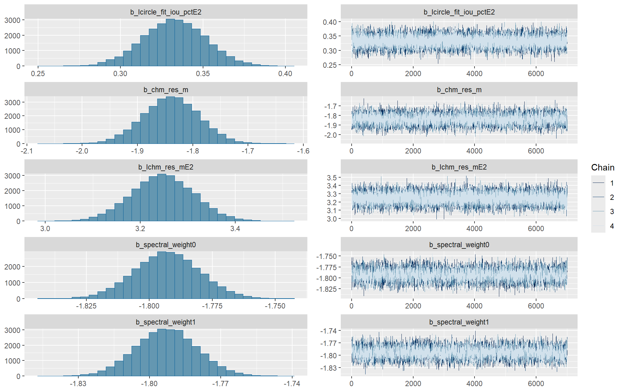

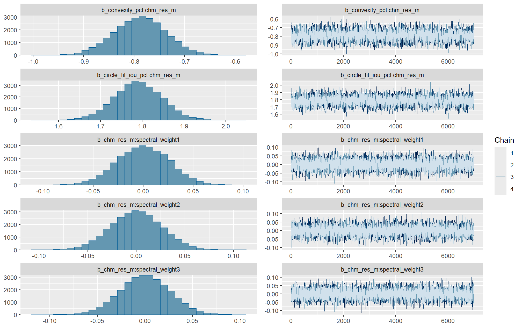
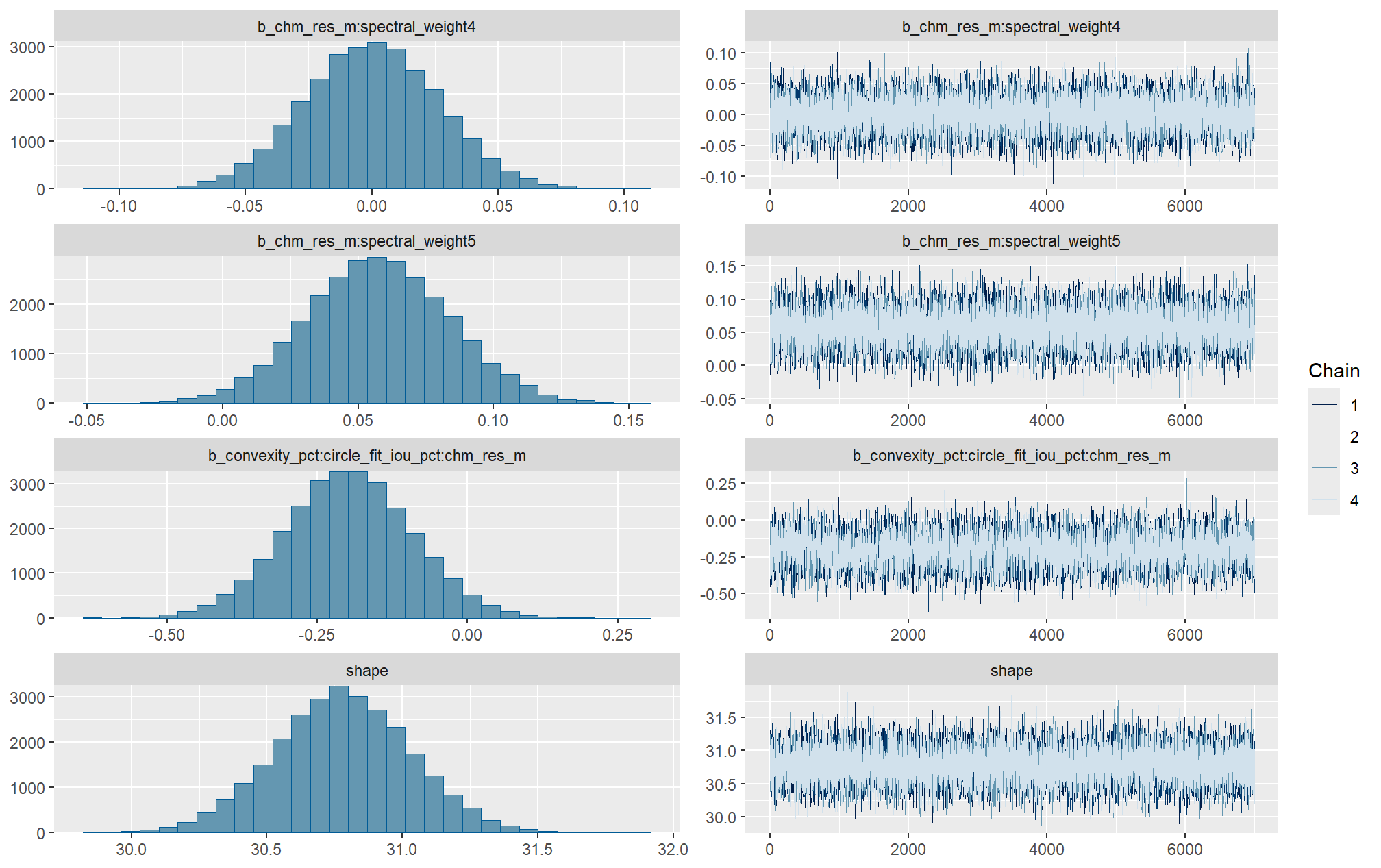
Sufficient convergence was checked with \(\hat{R}\) values near 1 (Brooks & Gelman, 1998).
in the plot below, \(\hat{R}\) values are colored using different shades (lighter is better). The chosen thresholds are somewhat arbitrary, but can be useful guidelines in practice (Gabry and Mahr 2025):
- light: below 1.05 (good)
- mid: between 1.05 and 1.1 (ok)
- dark: above 1.1 (too high)
check our \(\hat{R}\) values
brms::mcmc_plot(brms_height_mape_mod, type = "rhat_hist") +
ggplot2::scale_x_continuous(breaks = scales::breaks_extended(n = 6)) +
ggplot2::theme_light() +
ggplot2::theme(
legend.position = "top", legend.direction = "horizontal"
)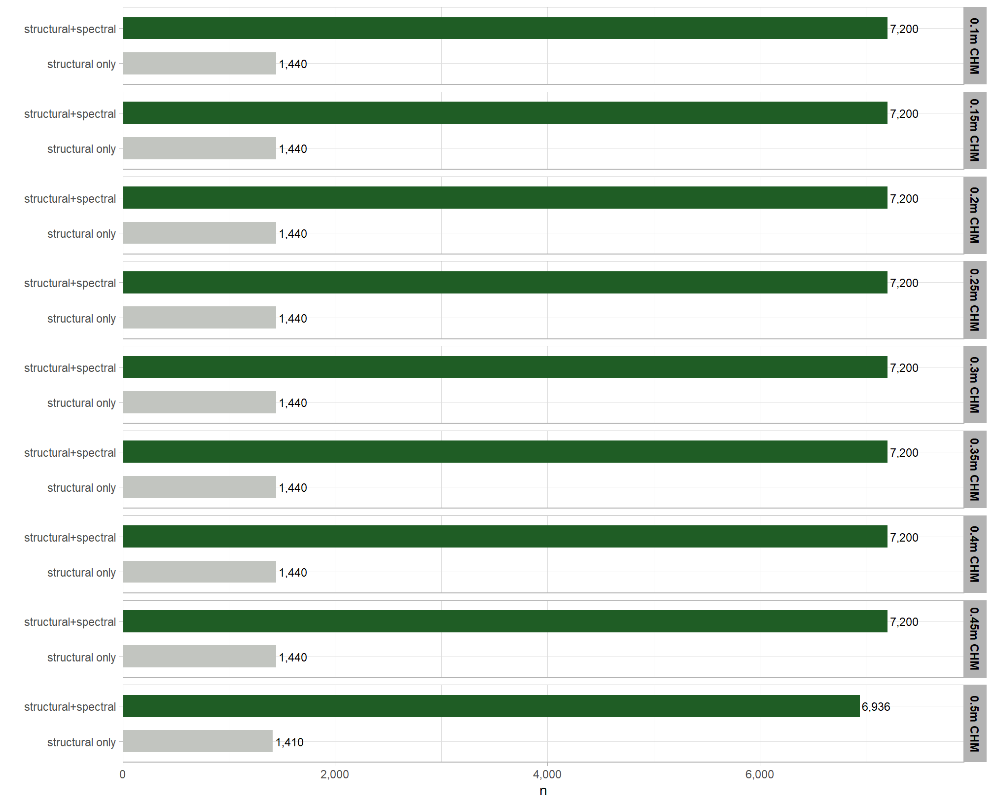
The effective length of an MCMC chain is indicated by the effective sample size (ESS), which refers to the sample size of the MCMC chain not to the sample size of the data where acceptable values allow “for reasonably accurate and stable estimates of the limits of the 95% HDI…If accuracy of the HDI limits is not crucial for your application, then a smaller ESS may be sufficient” (Kruschke 2015, p. 184)
Ratios of effective sample size (ESS) to total sample size with values are colored using different shades (lighter is better). A ratio close to “1” (no autocorrelation) is ideal, while a low ratio suggests the need for more samples or model re-parameterization. Efficiently mixing MCMC chains are important because they guarantee the resulting posterior samples accurately represent the true distribution of model parameters, which is necessary for reliable and precise estimation of parameter values and their associated uncertainties (credible intervals). The chosen thresholds are somewhat arbitrary, but can be useful guidelines in practice (Gabry and Mahr 2025):
- light: between 0.5 and 1 (high)
- mid: between 0.1 and 0.5 (good)
- dark: below 0.1 (low)
# and another effective sample size check
brms::mcmc_plot(brms_height_mape_mod, type = "neff_hist") +
# brms::mcmc_plot(brms_height_mape_mod, type = "neff") +
ggplot2::scale_x_continuous(limits = c(0,NA), breaks = scales::breaks_extended(n = 9)) +
# ggplot2::scale_color_discrete(drop = F) +
# ggplot2::scale_fill_discrete(drop = F) +
ggplot2::theme_light() +
ggplot2::theme(
legend.position = "top", legend.direction = "horizontal"
)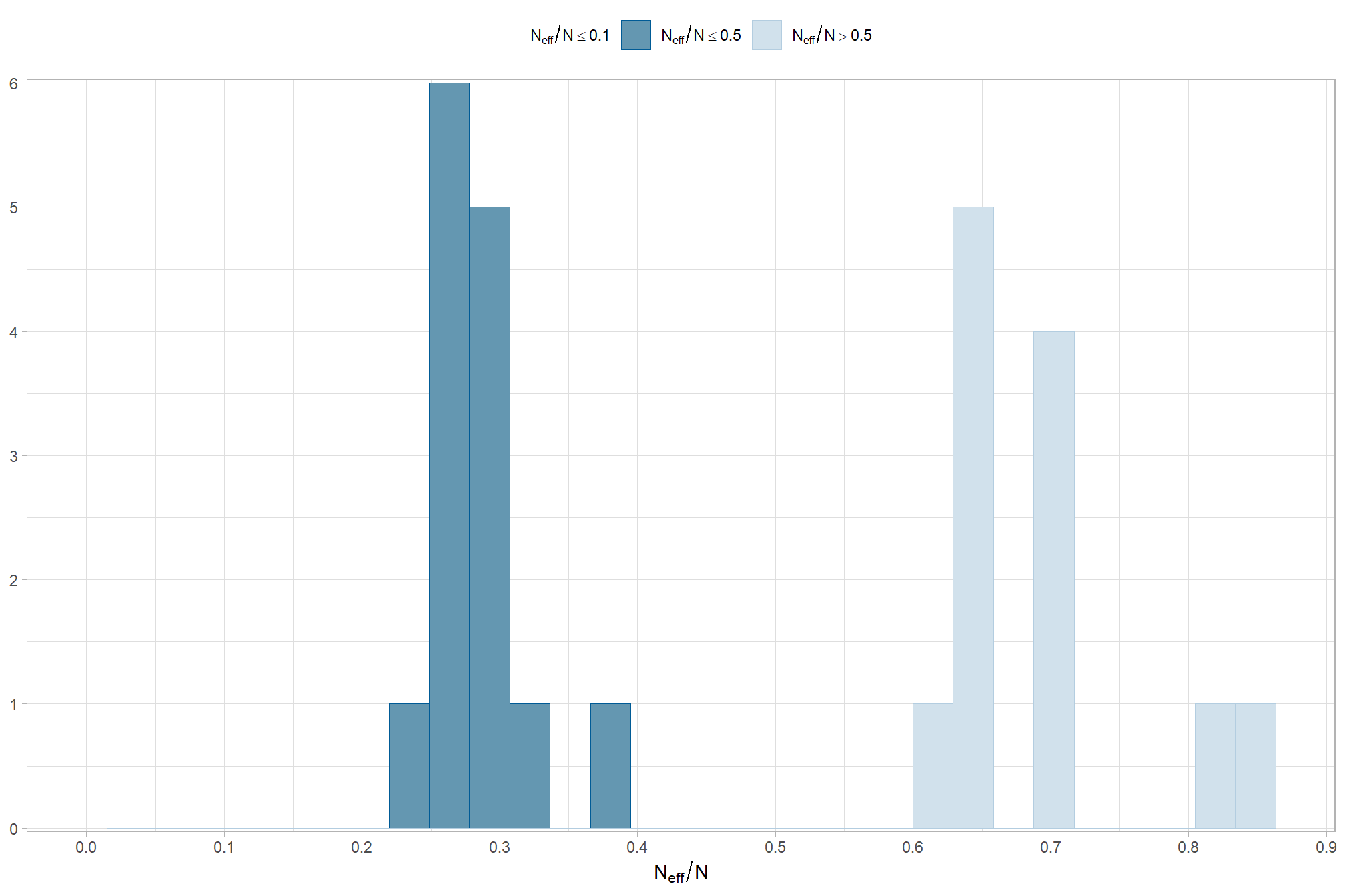
Posterior predictive checks were used to evaluate model goodness-of-fit by comparing data simulated from the model with the observed data used to estimate the model parameters (Hobbs & Hooten, 2015). Calculating the proportion of MCMC iterations in which the test statistic (i.e., mean and sum of squares) from the simulated data and observed data are more extreme than one another provides the Bayesian p-value. Lack of fit is indicated by a value close to 0 or 1 while a value of 0.5 indicates perfect fit (Hobbs & Hooten, 2015).
To learn more about this approach to posterior predictive checks, check out Gabry’s (2025) vignette, Graphical posterior predictive checks using the bayesplot package.
posterior-predictive check to make sure the model does an okay job simulating data that resemble the sample data. our objective is to construct the model such that it faithfully represents the data.
# posterior predictive check
brms::pp_check(
brms_height_mape_mod
, type = "dens_overlay"
, ndraws = 100
) +
ggplot2::labs(subtitle = "posterior-predictive check (overlaid densities)") +
ggplot2::theme_light() +
ggplot2::scale_y_continuous(NULL, breaks = NULL) +
ggplot2::theme(
legend.position = "top", legend.direction = "horizontal"
, legend.text = ggplot2::element_text(size = 14)
, plot.subtitle = ggplot2::element_text(size = 8)
, plot.title = ggplot2::element_text(size = 9)
)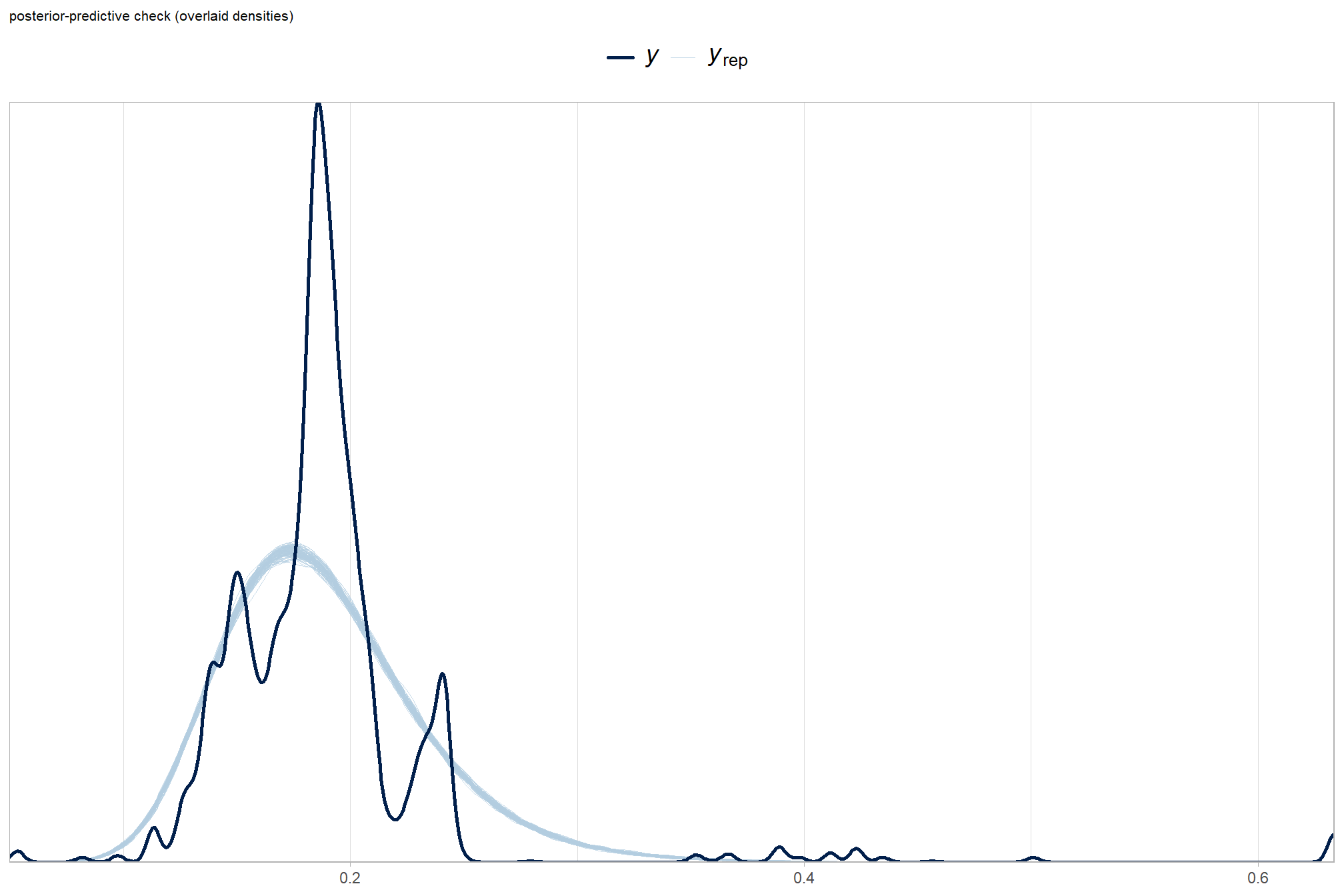
another way
brms::pp_check(brms_height_mape_mod, type = "ecdf_overlay", ndraws = 100) +
ggplot2::labs(subtitle = "posterior-predictive check (ECDF: empirical cumulative distribution function)") +
ggplot2::theme_light() +
ggplot2::theme(
legend.position = "top", legend.direction = "horizontal"
, legend.text = ggplot2::element_text(size = 14)
)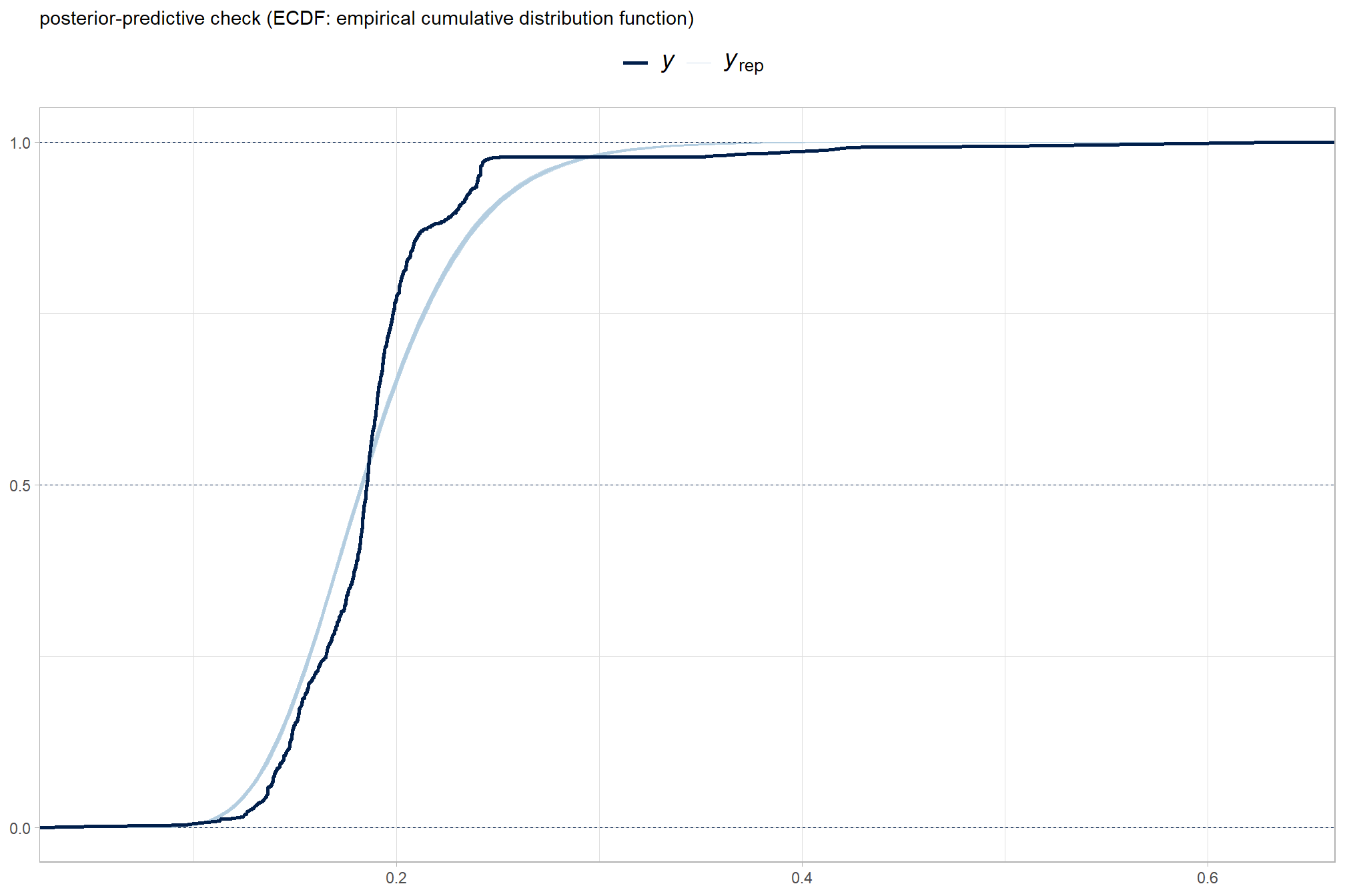
9.3.4 Conditional Effects
first, lets look at densities of the posterior samples per parameter
brms::mcmc_plot(brms_height_mape_mod, type = "dens") +
# ggplot2::theme_light() +
ggplot2::theme(
strip.text = ggplot2::element_text(size = 7.5, face = "bold", color = "black")
)
and we can look at the default coefficient plot that is commonly used in reporting coefficient “significance” in frequentist analysis
# easy way to get the default coeff plot
brms::mcmc_plot(brms_height_mape_mod, variable = "\\bb_", regex = T, type = "intervals")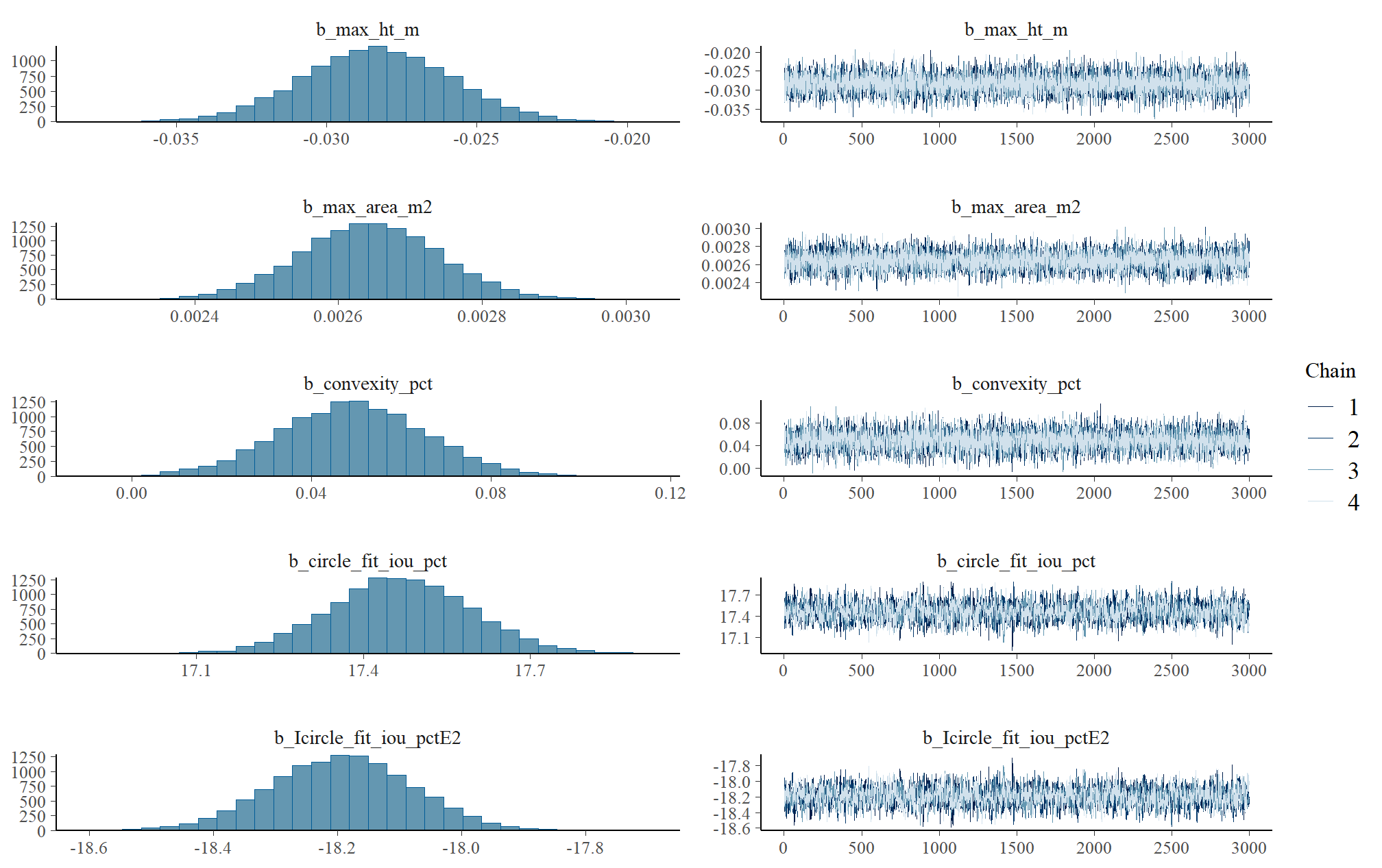
Regarding interactions and polynomial models like the one we use, McElreath (2015) notes:
parameters are the linear and square components of the curve, respectively. But that doesn’t make them transparent. You have to plot these model fits to understand what they are saying. (p. 112-113)
all of the interactions and the quadradic trend of this model combine to make these coefficients by themselves uninterpretable as the coefficients are only meaningful in the context of the other terms in the interaction or by adding the quadratic component
we can do this by checking for the main effects of the individual variables on Height MAPE (averages across all other effects)
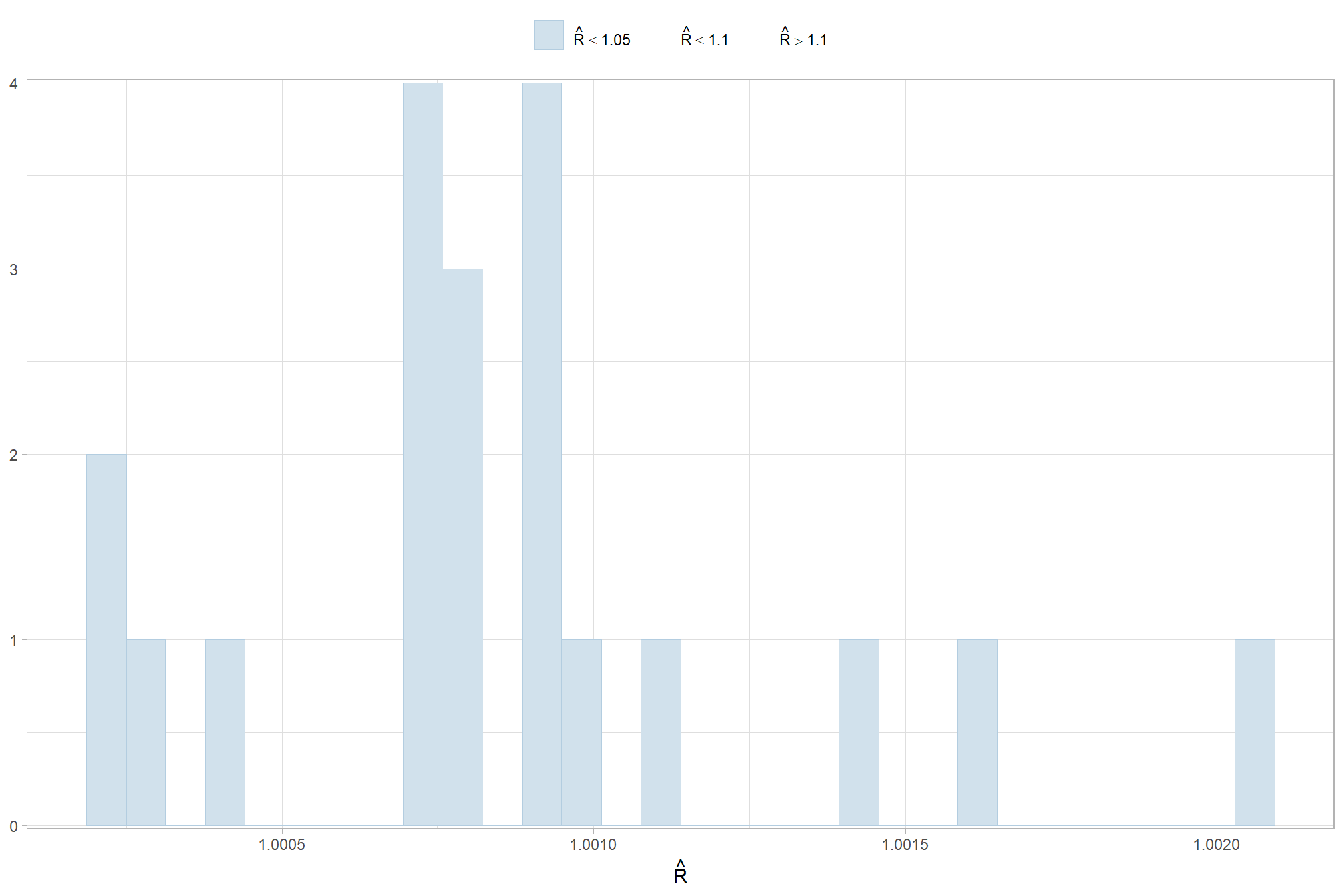
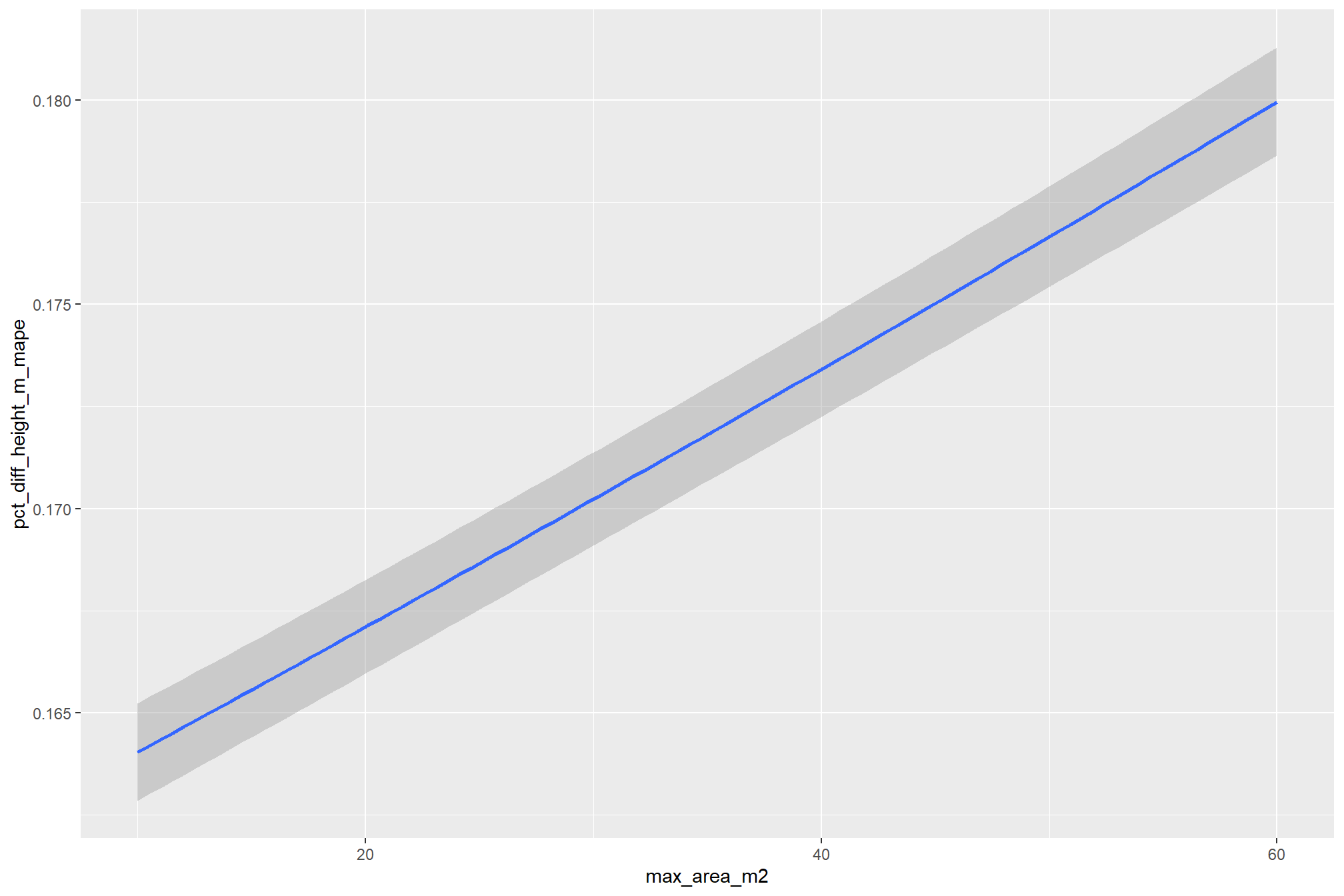
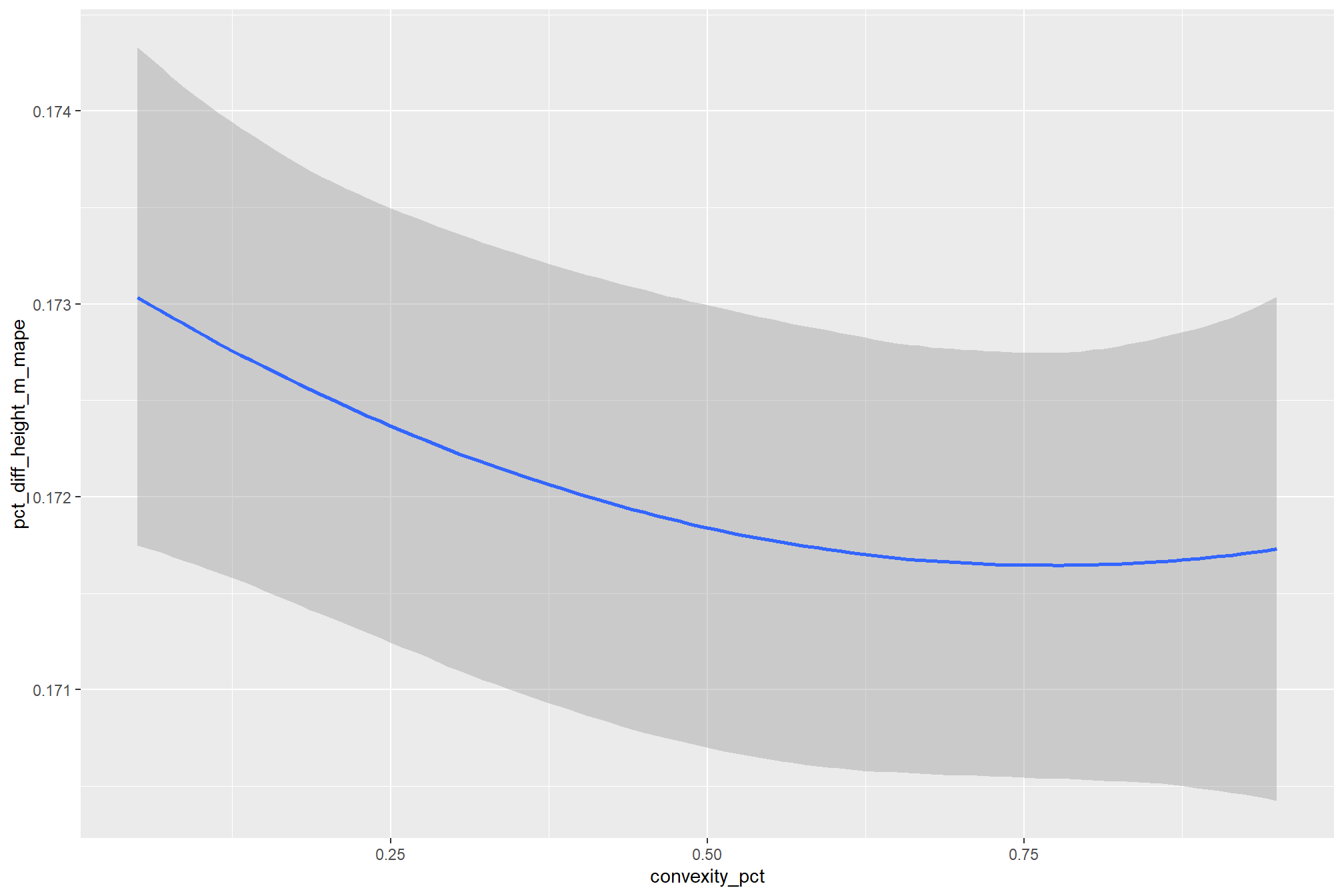
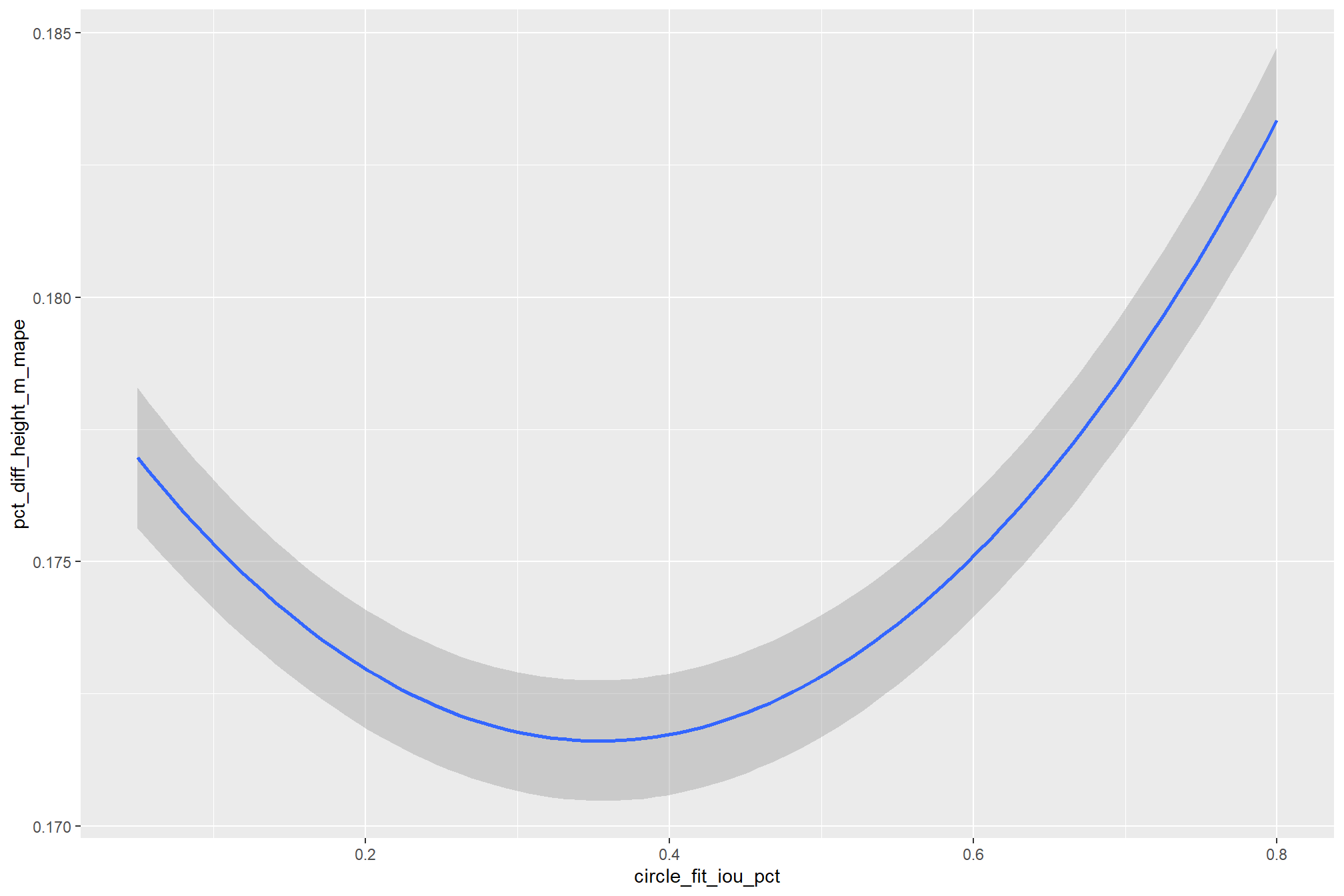
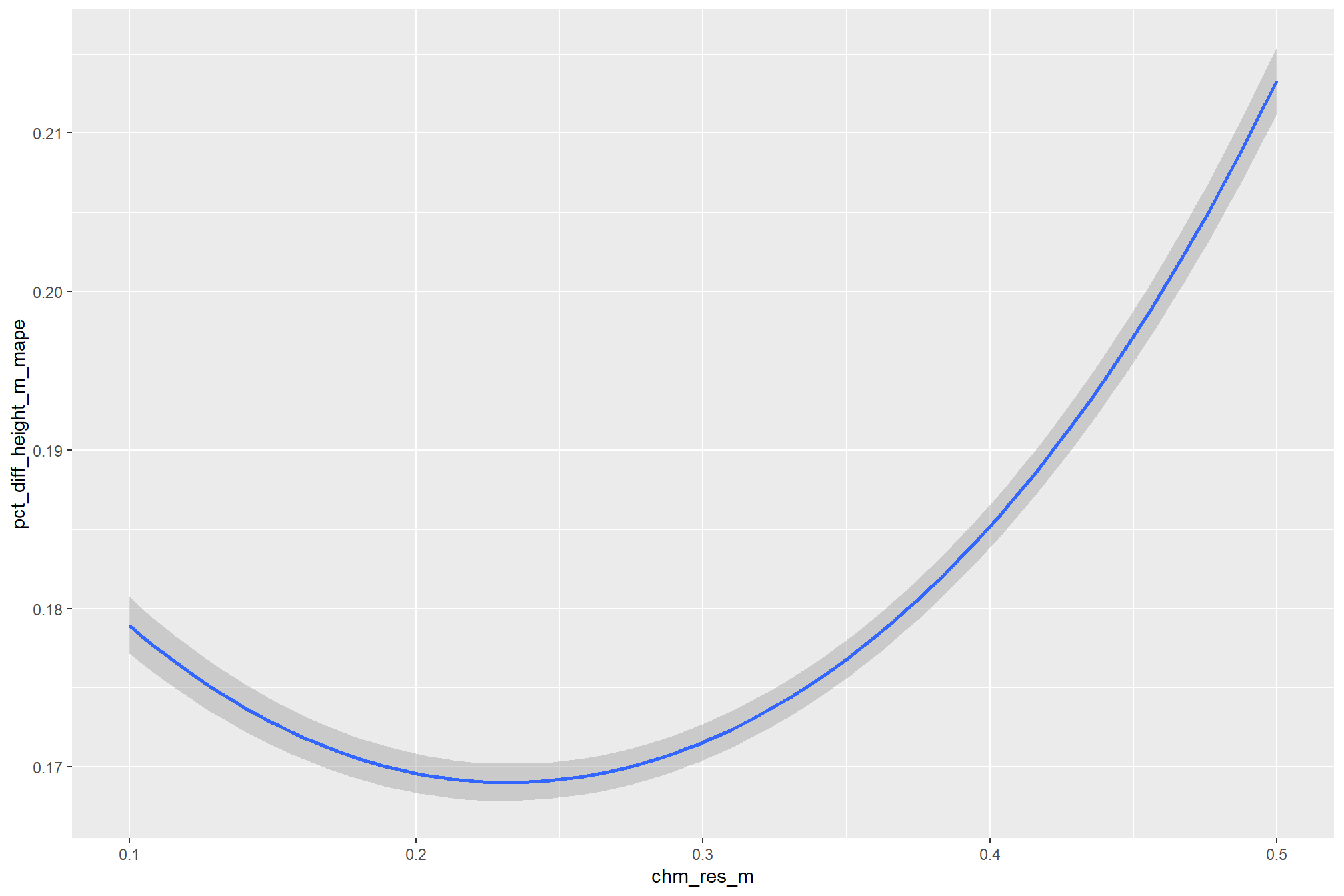
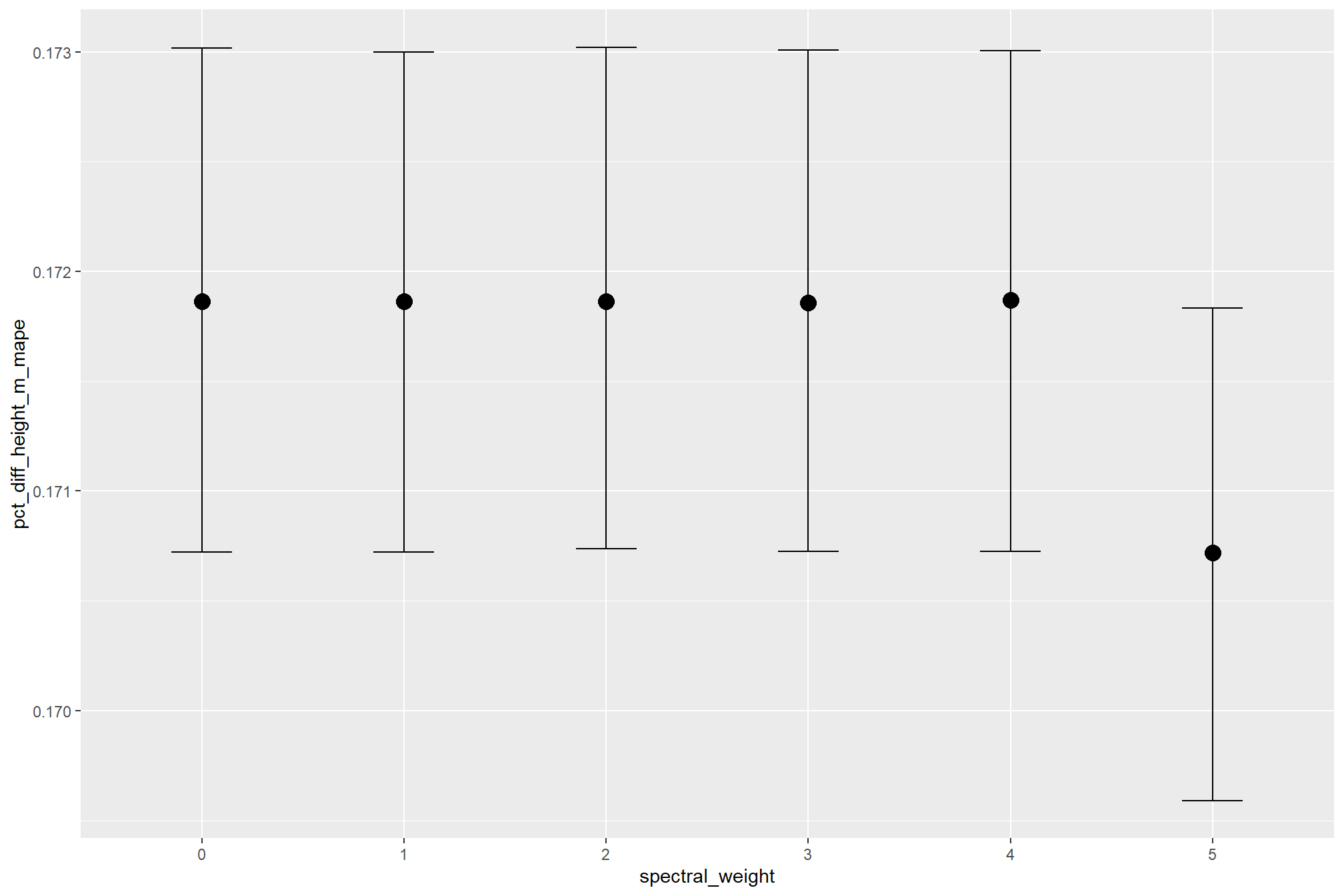
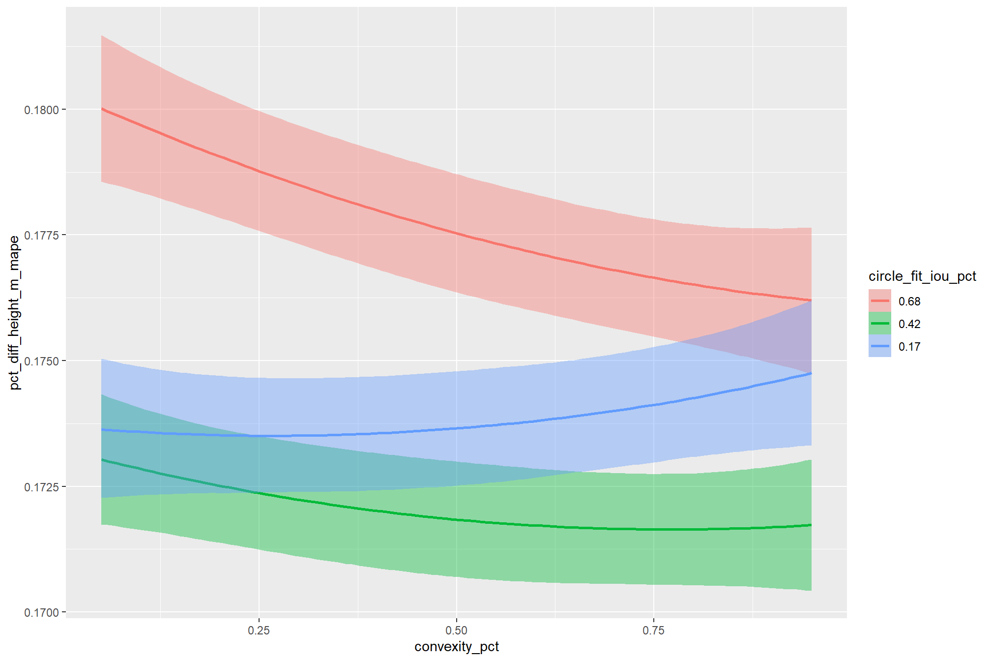
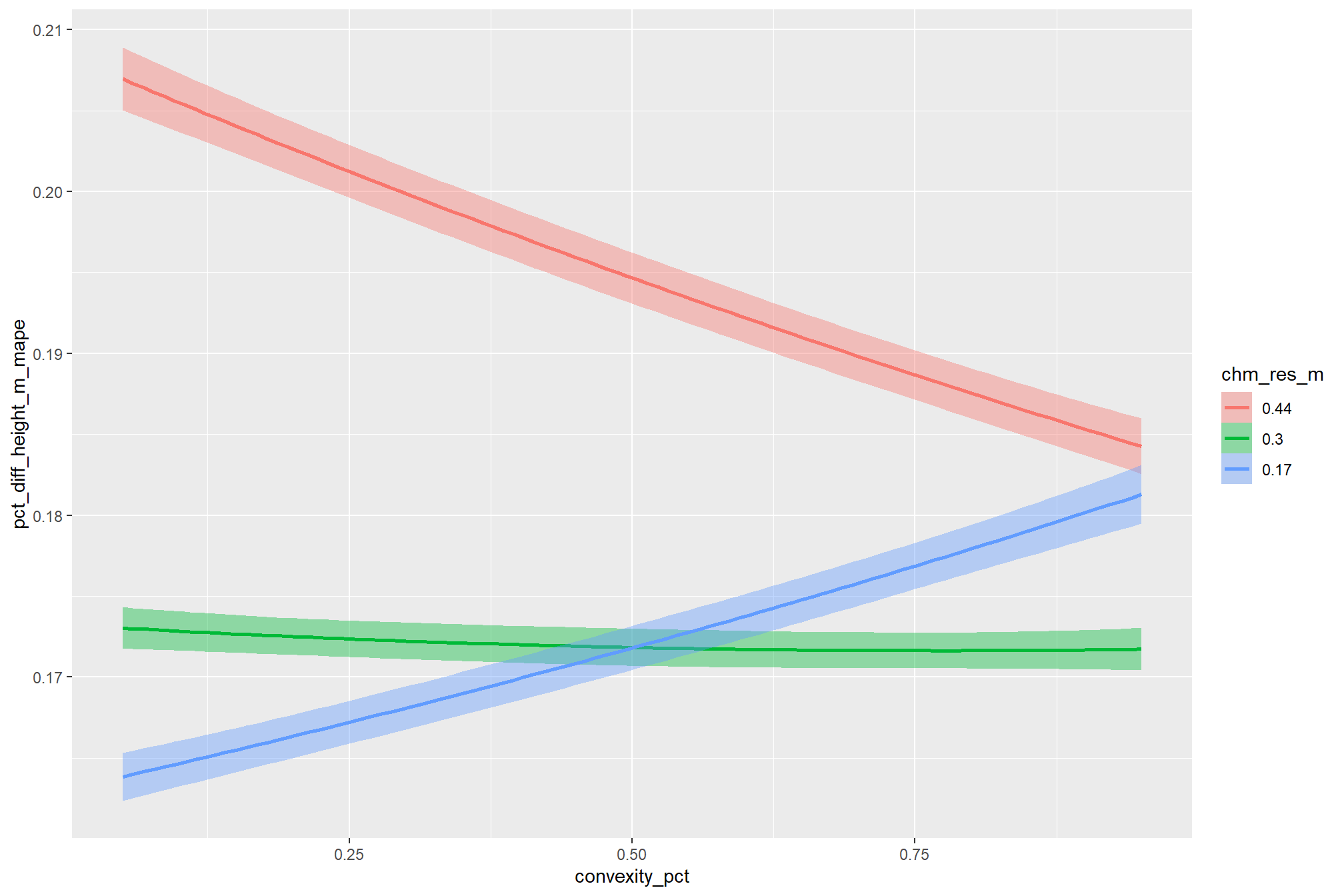
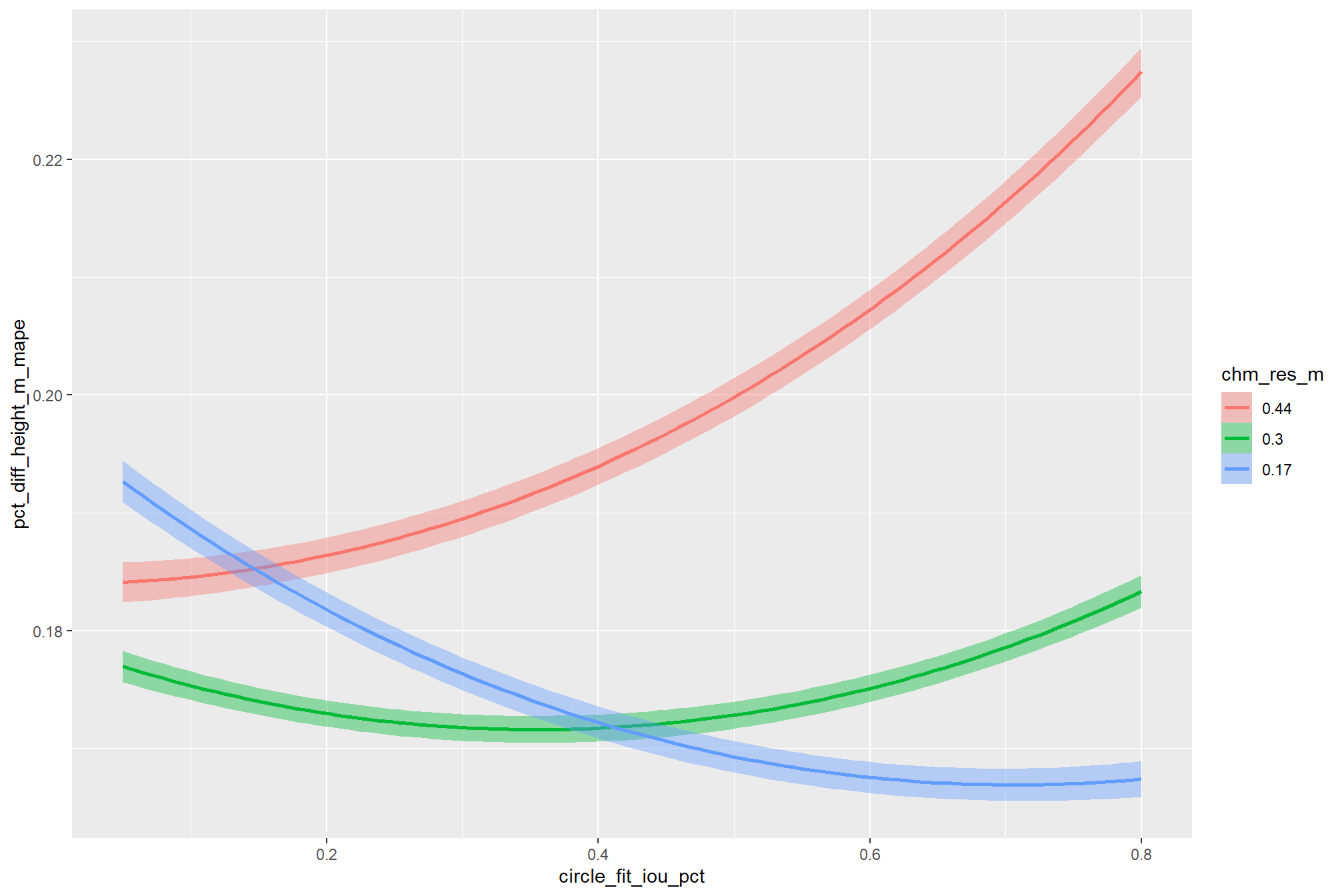
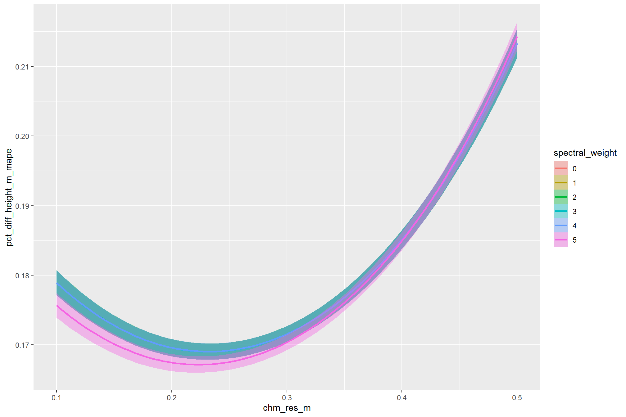
9.3.5 Posterior Predictive Expectation
we will test our hypotheses using the posterior distributions of the expected values (i.e., the posterior predictions of the mean) obtained via tidybayes::add_epred_draws(). our analysis will include two stages using parameter levels of the four structural parameters: max_ht_m, max_area_m2, convexity_pct, circle_fit_iou_pct. in practice, these values should be informed by the treatment prescription implemented on the ground.
In the first stage, we will fix the max_ht_m and max_area_m2 parameters at levels expected based on the treatment and slash pile construction prescription implemented on the ground. We will then explore the influence of the two geometric shape filtering parameters (circle_fit_iou_pct and convexity_pct) over different levels of the spectral_weight parameter and CHM resolution data.
In the second stage, we will fix all four structural parameters (max_ht_m, max_area_m2, convexity_pct, circle_fit_iou_pct) to explore the influence of the input data, which includes the presence or absence of spectral data and its weighting (i.e. spectral_weight) as well as the CHM resolution (chm_res_m). As in the first stage, the max_ht_m, max_area_m2 parameters will be fixed at expected levels based on the slash pile construction prescription while the convexity_pct, circle_fit_iou_pct are fixed at the optimal levels determined based on the Bayesian posterior predictive distribution of detection accuracy
as a reminder, here are those parameter levels
## Rows: 1
## Columns: 4
## $ circle_fit_iou_pct <dbl> 0.35
## $ convexity_pct      <dbl> 0.36
## $ max_ht_m           <dbl> 2.3
## $ max_area_m2        <dbl> 46
now we’ll get the posterior predictive draws but over a range of circle_fit_iou_pct and convexity_pct including the best setting
seq_temp <- seq(from = 0.05, to = 1.0, by = 0.1)
seq2_temp <- seq_temp[seq(1, length(seq_temp), by = 2)] # get every other element
# draws
draws_temp <-
# get the draws for levels of
# spectral_weight circle_fit_iou_pct convexity_pct
tidyr::crossing(
param_combos_spectral_ranked %>% dplyr::distinct(spectral_weight)
, circle_fit_iou_pct = seq_temp %>% unique()
, convexity_pct = seq_temp %>% unique()
, chm_res_m = seq(from = 0.1, to = 1.0, by = 0.1)
, max_ht_m = structural_params_settings$max_ht_m
, max_area_m2 = structural_params_settings$max_area_m2
) %>%
# dplyr::glimpse()
tidybayes::add_epred_draws(brms_height_mape_mod, ndraws = 1111) %>%
dplyr::rename(value = .epred) %>%
dplyr::mutate(
is_seq = (convexity_pct %in% seq_temp) & (circle_fit_iou_pct %in% seq_temp)
)
# # huh?
draws_temp %>% dplyr::glimpse()## Rows: 6,666,000
## Columns: 12
## Groups: spectral_weight, circle_fit_iou_pct, convexity_pct, chm_res_m, max_ht_m, max_area_m2, .row [6,000]
## $ spectral_weight <fct> 0, 0, 0, 0, 0, 0, 0, 0, 0, 0, 0, 0, 0, 0, 0, 0, 0, …
## $ circle_fit_iou_pct <dbl> 0.05, 0.05, 0.05, 0.05, 0.05, 0.05, 0.05, 0.05, 0.0…
## $ convexity_pct <dbl> 0.05, 0.05, 0.05, 0.05, 0.05, 0.05, 0.05, 0.05, 0.0…
## $ chm_res_m <dbl> 0.1, 0.1, 0.1, 0.1, 0.1, 0.1, 0.1, 0.1, 0.1, 0.1, 0…
## $ max_ht_m <dbl> 2.3, 2.3, 2.3, 2.3, 2.3, 2.3, 2.3, 2.3, 2.3, 2.3, 2…
## $ max_area_m2 <dbl> 46, 46, 46, 46, 46, 46, 46, 46, 46, 46, 46, 46, 46,…
## $ .row <int> 1, 1, 1, 1, 1, 1, 1, 1, 1, 1, 1, 1, 1, 1, 1, 1, 1, …
## $ .chain <int> NA, NA, NA, NA, NA, NA, NA, NA, NA, NA, NA, NA, NA,…
## $ .iteration <int> NA, NA, NA, NA, NA, NA, NA, NA, NA, NA, NA, NA, NA,…
## $ .draw <int> 1, 2, 3, 4, 5, 6, 7, 8, 9, 10, 11, 12, 13, 14, 15, …
## $ value <dbl> 0.1795179, 0.1804930, 0.1812731, 0.1823152, 0.18121…
## $ is_seq <lgl> TRUE, TRUE, TRUE, TRUE, TRUE, TRUE, TRUE, TRUE, TRU…9.3.5.1 Geometric shape regularity
let’s look at the influence of the parameters that control the geometric shape regularity filtering: circle_fit_iou_pct and convexity_pct. to do this, we will fix the max_ht_m and max_area_m2 parameters at levels expected based on the treatment and slash pile construction prescription implemented on the ground.
In the first stage, we will fix the max_ht_m and max_area_m2 parameters at levels expected based on the treatment and slash pile construction prescription implemented on the ground. We will then explore the influence of the two geometric shape filtering parameters (circle_fit_iou_pct and convexity_pct) over different levels of the spectral_weight parameter and CHM resolution data.
In the second stage, we will fix all four structural parameters (max_ht_m, max_area_m2, convexity_pct, circle_fit_iou_pct) to explore the influence of the input data, which includes the presence or absence of spectral data and its weighting (i.e. spectral_weight) as well as the CHM resolution (chm_res_m). As in the first stage, the max_ht_m, max_area_m2 parameters will be fixed at expected levels based on the slash pile construction prescription while the convexity_pct, circle_fit_iou_pct will be fixed at the optimal levels determined based on the Bayesian posterior predictive distribution of detection accuracy
9.3.5.1.1 circle_fit_iou_pct
we need to look at the influence of circle_fit_iou_pct in the context of the other terms in the interaction
draws_temp %>%
dplyr::ungroup() %>%
dplyr::filter(
is_seq
, chm_res_m %in% seq(0.1,0.5,by=0.2)
, convexity_pct %in% seq2_temp
) %>%
dplyr::mutate(convexity_pct = factor(convexity_pct, ordered = T)) %>%
ggplot2::ggplot(mapping = ggplot2::aes(x = circle_fit_iou_pct, y = value, color = convexity_pct)) +
tidybayes::stat_lineribbon(
point_interval = "median_hdi", .width = c(0.95)
, lwd = 1.1
, fill = NA
) +
ggplot2::facet_grid(cols = dplyr::vars(spectral_weight), rows = dplyr::vars(chm_res_m), labeller = "label_both", scales = "free_y") +
ggplot2::scale_fill_brewer(palette = "Greys") +
ggplot2::scale_color_viridis_d(option = "mako", begin = 0.6, end = 0.1) +
ggplot2::scale_x_continuous(limits = c(0,1)) +
ggplot2::scale_y_continuous(labels = scales::percent) +
ggplot2::labs(
title = "conditional effect of `circle_fit_iou_pct` on Height MAPE"
# , subtitle = "Faceted by spectral_weight and chm_res_m"
, x = "`circle_fit_iou_pct`"
, y = "Height MAPE"
, color = "`convexity_pct`"
) +
ggplot2::theme_light() +
ggplot2::theme(
legend.position = "top"
, strip.text.x = ggplot2::element_text(size = 10, color = "black", face = "bold")
, strip.text.y = ggplot2::element_text(size = 10, color = "black", face = "bold")
) +
ggplot2::guides(
color = ggplot2::guide_legend(override.aes = list(shape = 15, lwd = 8, fill = NA))
, fill = "none"
)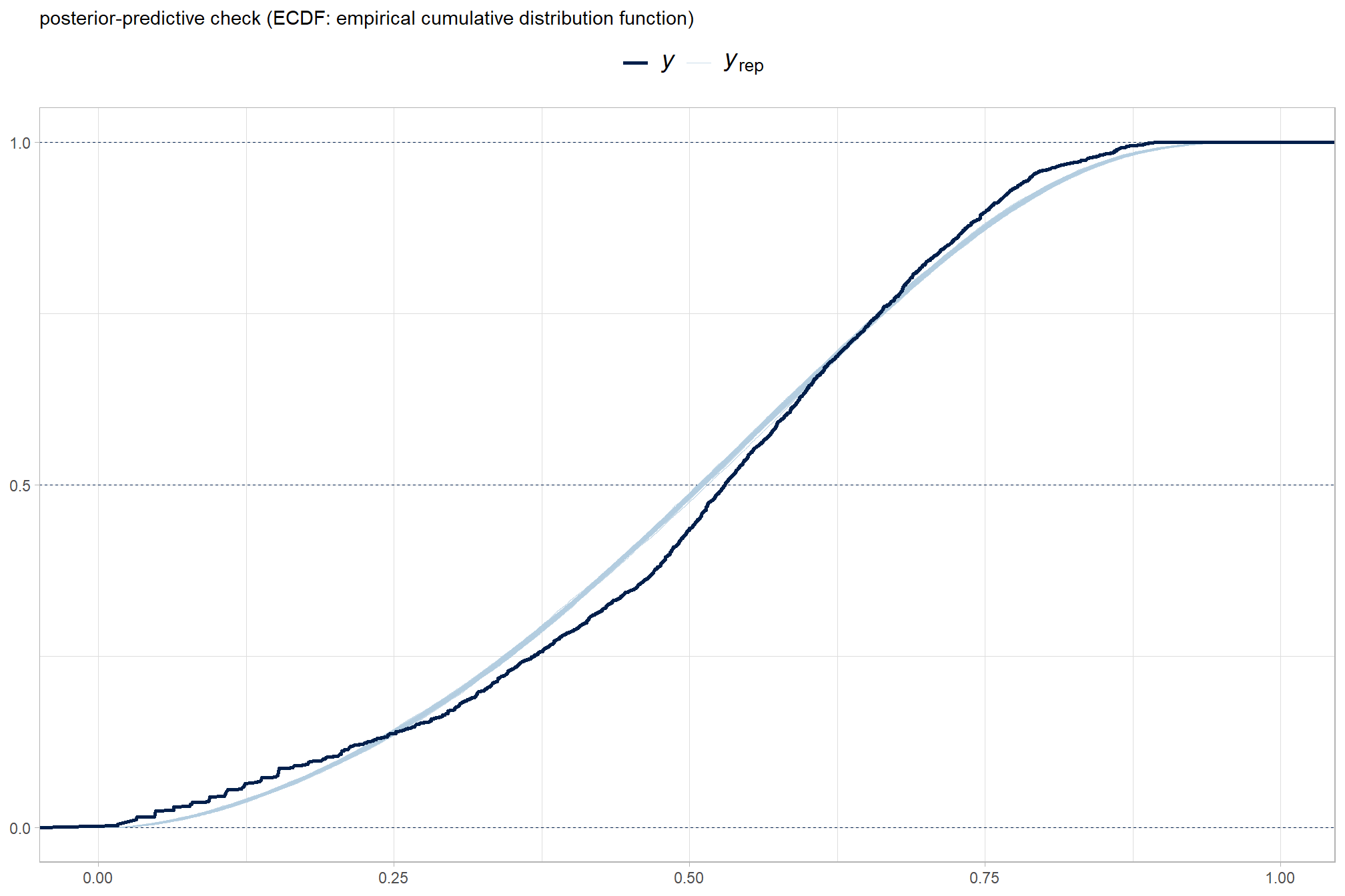
For all of these faceted plots, note the variation in the y-axis (Predicted Height MAPE) range across different CHM resolution levels. The influence of the circle_fit_iou_pct parameter on the Height MAPE is dependent on the CHM resolution but, unlike diameter quantification, its trend does not change based on the convexity_pct parameter setting. The magnitude of this influence decreases with finer data: for the finest resolution CHM data (0.1m), changes in circle_fit_iou_pct only shift the MAPE by approximately 6 percentage points, while for the coarsest resolution CHM data (0.5m), the shift in MAPE is approximately 11 percentage points as circle_fit_iou_pct is varied. There is a notable shift in the influence of the circle_fit_iou_pct parameter as CHM resolution moves from fine to coarse. With fine resolution CHM data (0.1m), height quantification accuracy improves (MAPE decreases) as the circle_fit_iou_pct parameter is increased toward its highest setting of ‘1’, with improvements stabilizing around 0.6. For moderate resolution CHM data (0.3m), the parabolic relationship between the circle_fit_iou_pct parameter and the Height MAPE becomes evident. Height accuracy is optimized at low-intermediate levels of the circle_fit_iou_pct parameter (e.g., 0.25–0.5), and height quantification accuracy steeply declines (MAPE increases) for values set above this level. For coarse resolution CHM data (0.5m), there is a consistent decrease in height quantification accuracy (increase in MAPE) as the circle_fit_iou_pct parameter is increased toward its highest setting of ‘1’; this trend is opposite of what was found for the fine resolution CHM data. With coarse resolution CHM data, the best height accuracy is achieved at the lowest circle_fit_iou_pct parameter settings, near ‘0’. These seemingly conflicting trends likely occur because the coarser resolution CHM data smoothes out variation in height from the aerial point cloud, while the variability in the elevation profile within a detected slash pile is retained when using finer resolution data.
9.3.5.1.2 convexity_pct
we need to look at the influence of convexity_pct in the context of the other terms in the interaction
draws_temp %>%
dplyr::ungroup() %>%
dplyr::filter(
is_seq
, chm_res_m %in% seq(0.1,0.5,by=0.2)
, circle_fit_iou_pct %in% seq2_temp
) %>%
dplyr::mutate(circle_fit_iou_pct = factor(circle_fit_iou_pct, ordered = T)) %>%
ggplot2::ggplot(mapping = ggplot2::aes(x = convexity_pct, y = value, color = circle_fit_iou_pct)) +
tidybayes::stat_lineribbon(
point_interval = "median_hdi", .width = c(0.95)
, lwd = 1.1
, fill = NA
) +
ggplot2::facet_grid(cols = dplyr::vars(spectral_weight), rows = dplyr::vars(chm_res_m), labeller = "label_both", scales = "free_y") +
ggplot2::scale_fill_brewer(palette = "Greys") +
ggplot2::scale_color_viridis_d(option = "magma", begin = 0.5, end = 0.1) +
ggplot2::scale_x_continuous(limits = c(0,1)) +
ggplot2::scale_y_continuous(labels = scales::percent) +
ggplot2::labs(
title = "conditional effect of `convexity_pct` on Height MAPE"
# , subtitle = "Faceted by spectral_weight and chm_res_m"
, x = "`convexity_pct`"
, y = "Height MAPE"
, color = "`circle_fit_iou_pct`"
) +
ggplot2::theme_light() +
ggplot2::theme(
legend.position = "top"
, strip.text.x = ggplot2::element_text(size = 10, color = "black", face = "bold")
, strip.text.y = ggplot2::element_text(size = 10, color = "black", face = "bold")
) +
ggplot2::guides(
color = ggplot2::guide_legend(override.aes = list(shape = 15, lwd = 8, fill = NA))
, fill = "none"
)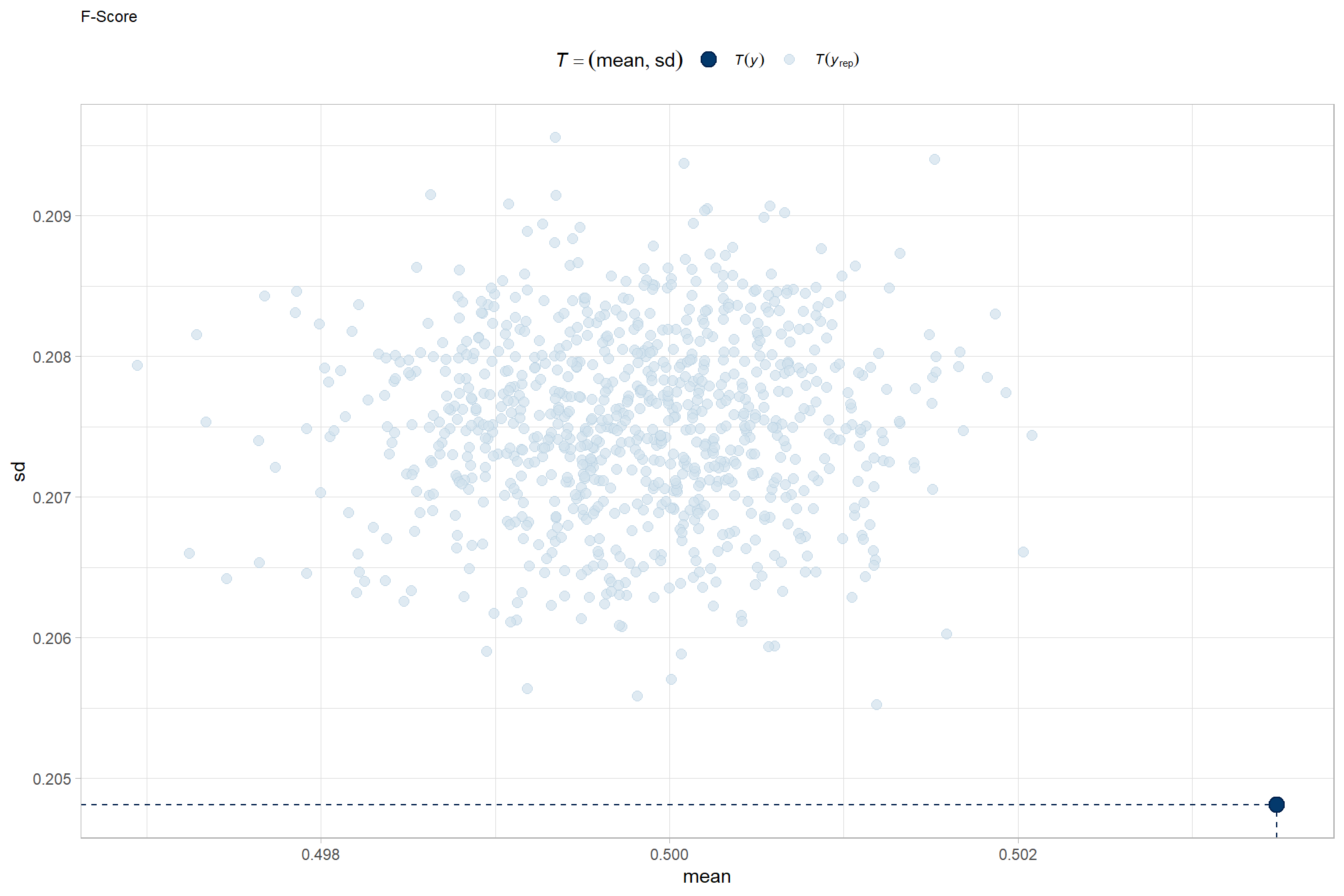
The model shows that the influence of the convexity_pct parameter on the Height MAPE is primarily conditional on the CHM resolution. The circle_fit_iou_pct parameter further influences the relationship between convexity_pct and height quantification accuracy but only at intermediate CHM resolutions (0.3m). Conversely, at the finest (0.1m) and coarsest (0.5m) CHM data levels, the circle_fit_iou_pct parameter does not alter the relationship between convexity_pct and Height MAPE but alters the magnitude of the influence. The magnitude of the convexity_pct parameter’s influence on Height MAPE is lowest for intermediate CHM resolutions (0.3m), with changes in the parameter only resulting in approximately 1.5 percentage point shifts in MAPE. The influence is significantly larger for other resolutions, causing a 6 percentage point shift over the convexity_pct range at finer resolutions (e.g. 0.1m) and a 10 percentage point influence at coarser resolutions (e.g. 0.5m). There is a notable shift in the optimal trend of the convexity_pct parameter as CHM resolution changes. With fine resolution CHM data (0.1m), height quantification accuracy improves (MAPE decreases) in a very linear trend as the convexity_pct parameter is decreased toward its lowest setting of ‘0’. This indicates that allowing for less regular (more concave/less smooth) segments yields better height accuracy at the finest resolution. This trend reverses for coarse resolution CHM data (0.5m), where there is a consistent decrease in height quantification accuracy (increase in MAPE) as the convexity_pct parameter is decreased toward its lowest setting of ‘0’. With coarse resolution CHM data, the best height accuracy is achieved at the highest convexity_pct parameter settings, near ‘1’. This suggests that at coarser resolutions, a very strict shape requirement is necessary to minimize errors in height estimation. Additionally, for coarser resolution data, the penalty in height quantification accuracy for decreasing convexity_pct toward 0 is steeper when the circle_fit_iou_pct parameter is set to higher levels (e.g., greater than 0.65) than when circle_fit_iou_pct is set to lower values (e.g., less than 0.25). This heightened penalty occurs because simultaneously requiring a pile to be highly circular (circle_fit_iou_pct high) and allowing it to be highly irregular (convexity_pct low) introduces high geometric uncertainty into the segmented area used for height calculation, making such a parameter combination unlikely to be applicable for optimizing height quantification accuracy using this pile detection method.
9.3.5.1.3 Optimizing geometric filtering
Given the complexity of our model, which includes a non-linear link function and parameter interactions, calculating the optimal parameter values by solving for them algebraically from the model’s coefficients would be prone to error. instead, we can use a robust Bayesian approach that leverages the model’s posterior predictive distribution. This method is powerful because it inherently accounts for all sources of model uncertainty.
first, we’ll generate a large number of predictions across a fine grid of parameter values (e.g. in steps of 0.01) for each posterior draw of the model coefficients. we’ll generate a large number (e.g. 1000+) of posterior predictive draws for each combination of parameter values. for each posterior predictive draw, we’ll then identify the parameter combination that maximizes the Height MAPE and we’ll be left with a posterior distribution of optimal parameter combinations.
this approach demonstrates a key advantage of the Bayesian framework, allowing us to ask complex questions and find the most probable optimal parameter combination while fully accounting for uncertainty.
note, we only extract draws based on not using any spectral data (i.e. spectral_weight = 0) to save on plotting space and because we expect form quantification to only be minimally influenced by the inclusion of spectral data
# let's get the draws at a very granular level
vertex_draws_temp <-
tidyr::crossing(
param_combos_spectral_ranked %>%
dplyr::filter(spectral_weight=="0") %>%
dplyr::distinct(spectral_weight, spectral_weight_fact)
, circle_fit_iou_pct = seq(from = 0.0, to = 1, by = 0.01) # very granular to identify vertex
, convexity_pct = seq(from = 0.0, to = 1, by = 0.02) # very granular to identify vertex
, chm_res_m = seq(0.1,0.5,by=0.1)
, max_ht_m = structural_params_settings$max_ht_m
, max_area_m2 = structural_params_settings$max_area_m2
) %>%
tidybayes::add_epred_draws(brms_height_mape_mod, ndraws = 1000, value = "value") %>%
dplyr::ungroup() %>%
# for each draw, get the highest Height MAPE by chm_res_m, spectral_weight
# which we'll use to identify the optimal circle_fit_iou_pct,convexity_pct settings
# these are essentially "votes" based on likelihood
dplyr::group_by(
.draw
, chm_res_m, spectral_weight
) %>%
dplyr::arrange(value,circle_fit_iou_pct,convexity_pct) %>% # notice the ascending sort of value (mape) here to take the lowest
dplyr::slice(1)
# vertex_draws_temp %>% dplyr::glimpse() # this thing is hugeplot the posterior distribution of optimal parameter setting for circle_fit_iou_pct
vertex_draws_temp %>%
dplyr::filter(
chm_res_m %in% seq(0.1,0.5,by=0.1)
) %>%
dplyr::ungroup() %>%
ggplot2::ggplot(mapping = ggplot2::aes(x = circle_fit_iou_pct)) +
tidybayes::stat_dotsinterval(
point_interval = "median_hdci", .width = c(0.95)
, quantiles = 100
, point_size = 3
) +
ggplot2::facet_grid(
cols = dplyr::vars(spectral_weight)
, rows = dplyr::vars(chm_res_m)
, scales = "free_y"
, labeller = "label_both"
, axes = "all_x"
) +
ggplot2::scale_x_continuous(limits = c(0,1)) +
# ggplot2::scale_x_continuous(limits = c(0,1), breaks = scales::breaks_extended(6)) +
ggplot2::scale_y_continuous(NULL, breaks = NULL) +
ggplot2::theme_light() +
ggplot2::theme(
strip.text.x = ggplot2::element_text(size = 10, color = "black", face = "bold")
, strip.text.y = ggplot2::element_text(size = 8, color = "black", face = "bold")
, axis.text.x = ggplot2::element_text(size = 8)
)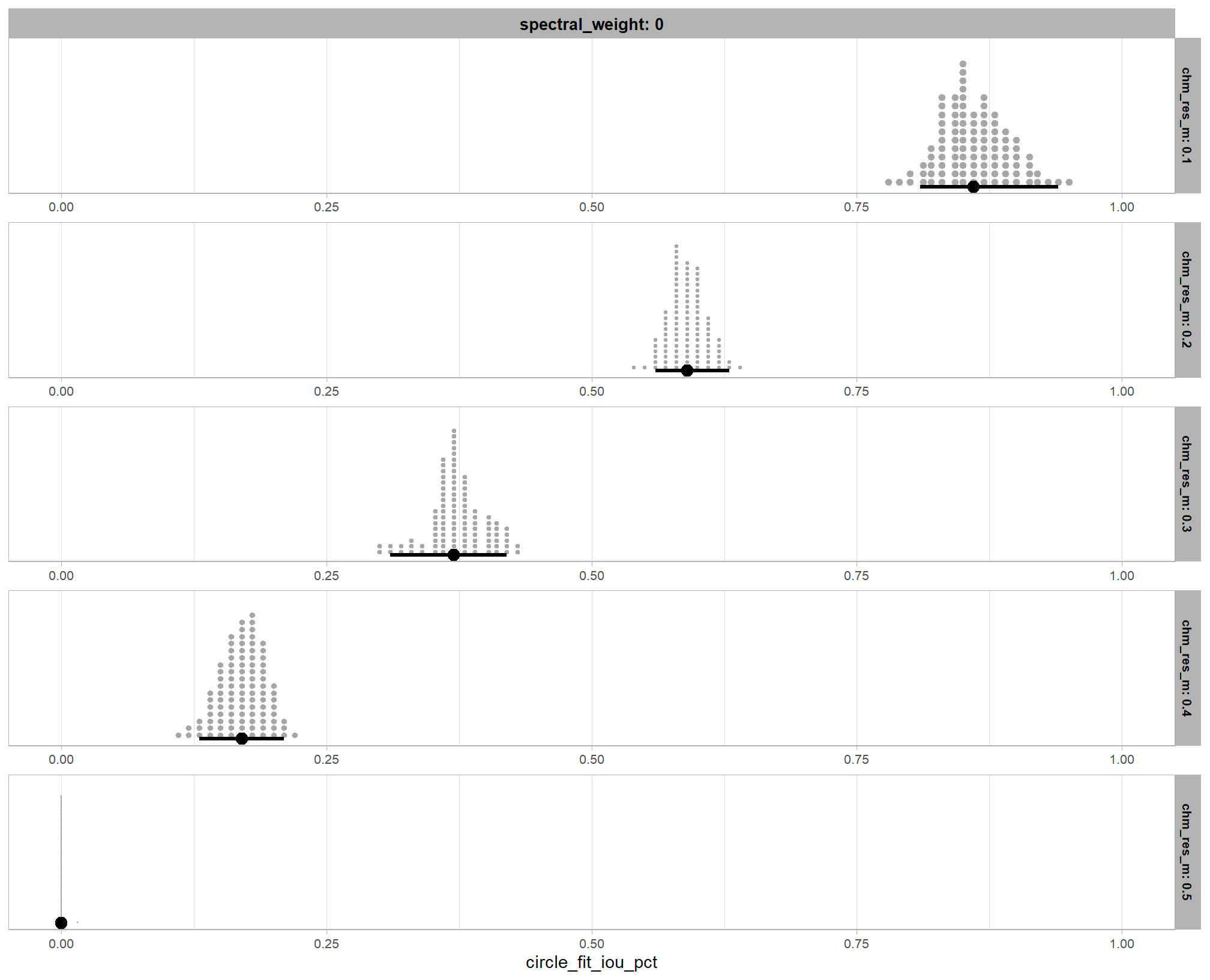
like we saw above, the optimal circle_fit_iou_pct for maximizing Height quantification accuracy shifts from higher (e.g. ~0.6-0.9) for fine resolution CHM data (e.g. <=0.2m) to lower (e.g. <0.25) for coarse resolution CHM data (e.g >=0.4m)
plot the posterior distribution of optimal parameter setting for convexity_pct
vertex_draws_temp %>%
dplyr::filter(
chm_res_m %in% seq(0.1,0.5,by=0.1)
) %>%
dplyr::ungroup() %>%
ggplot2::ggplot(mapping = ggplot2::aes(x = convexity_pct)) +
tidybayes::stat_dotsinterval(
point_interval = "median_hdci", .width = c(0.95)
, quantiles = 100
, point_size = 3
) +
ggplot2::facet_grid(
cols = dplyr::vars(spectral_weight)
, rows = dplyr::vars(chm_res_m)
, scales = "free_y"
, labeller = "label_both"
, axes = "all_x"
) +
ggplot2::scale_x_continuous(limits = c(0,1)) +
ggplot2::scale_y_continuous(NULL, breaks = NULL) +
ggplot2::theme_light() +
ggplot2::theme(
strip.text.x = ggplot2::element_text(size = 10, color = "black", face = "bold")
, strip.text.y = ggplot2::element_text(size = 8, color = "black", face = "bold")
)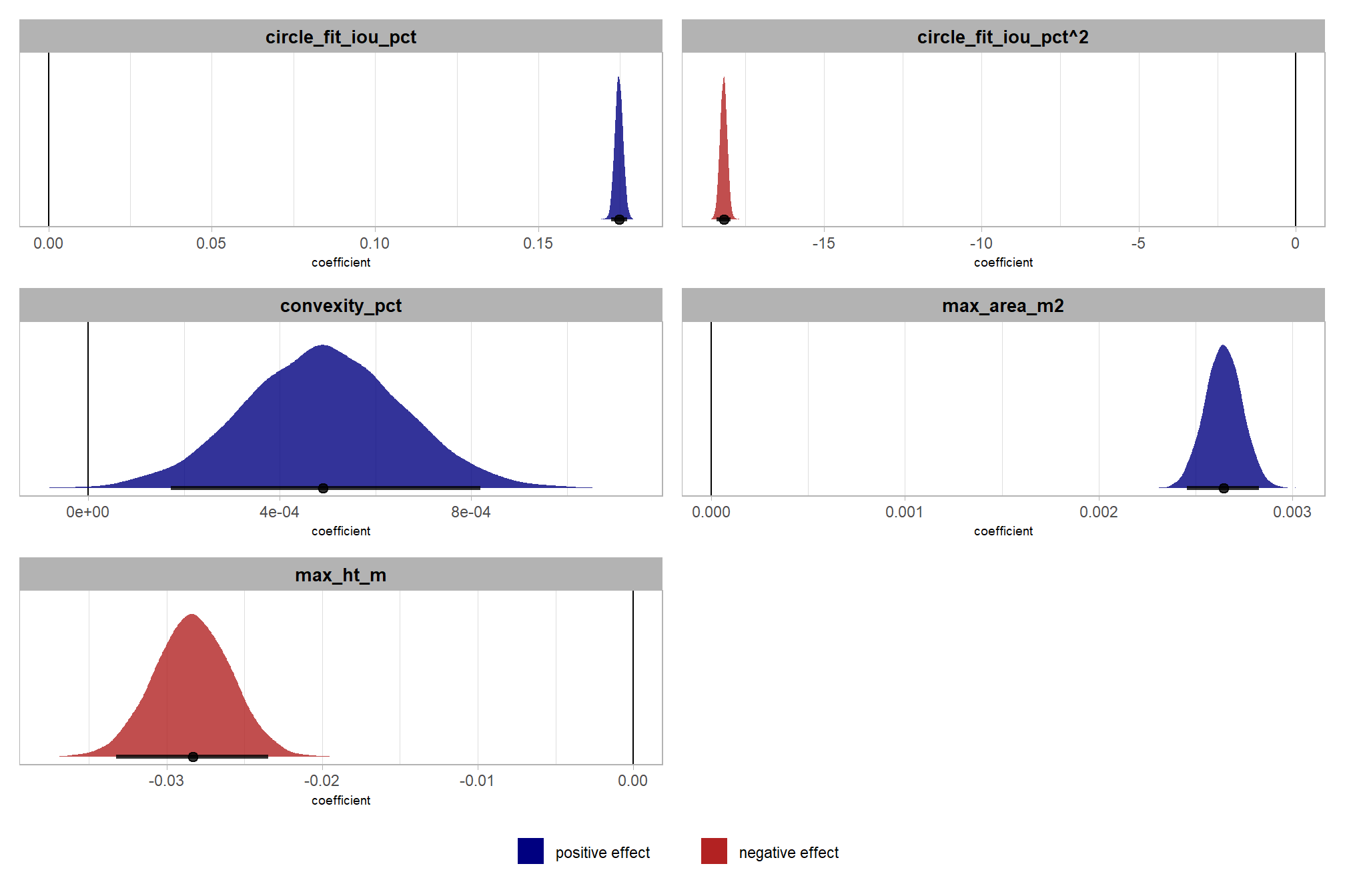
when the circle_fit_iou_pct parameter is optimized, the influence of convexity_pct on form quantification accuracy is dependent on the CHM resolution. only for the finest resolution CHM data (i.e. 0.1m) tested, the model’s predictions indicate with high certainty that the optimal convexity_pct is its minimum value of ‘0’. for intermediate resolution CHM data (e.g. 0.3m), the 95% HDI for the optimal convexity_pct spans the entire 0-1 range, indicating the model is not confident in any specific setting. for the coarsest resolution CHM data (i.e. 0.5m) tested, the model’s predictions indicate with high certainty that the optimal convexity_pct is its maximum value of ‘1’
we can look at this another way, check it
vertex_draws_temp %>%
dplyr::filter(
chm_res_m %in% seq(0.1,0.5,by=0.1)
) %>%
dplyr::ungroup() %>%
ggplot2::ggplot(mapping = ggplot2::aes(y = convexity_pct, x = circle_fit_iou_pct)) +
# geom_point(alpha=0.2) +
ggplot2::geom_jitter(alpha=0.2, height = .01, width = .01) +
ggplot2::facet_grid(
cols = dplyr::vars(spectral_weight)
, rows = dplyr::vars(chm_res_m)
# , scales = "free_y"
, labeller = "label_both"
) +
ggplot2::scale_y_continuous(limits = c(0,1)) +
ggplot2::scale_x_continuous(limits = c(0,1)) +
ggplot2::theme_light() +
ggplot2::theme(
strip.text.x = ggplot2::element_text(size = 10, color = "black", face = "bold")
, strip.text.y = ggplot2::element_text(size = 8, color = "black", face = "bold")
)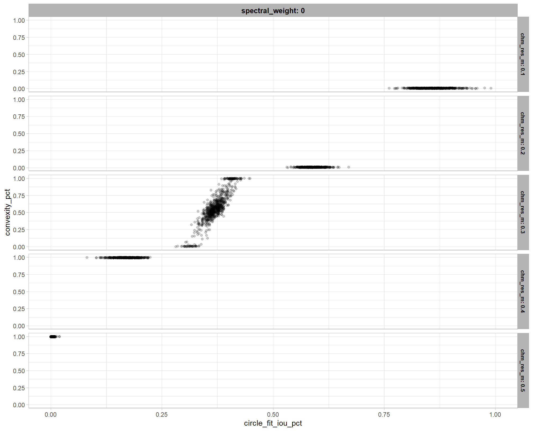
note, in the plot above, we slightly “jitter” the points so that they are visible where they would otherwise be stacked on top of each other and only look like a few points instead of the 1000 draws from the posterior we used
let’s table the HDI of the optimal values
# summarize it
vertex_draws_temp <-
  vertex_draws_temp %>%
  dplyr::group_by(
    chm_res_m, spectral_weight
  ) %>%
  dplyr::summarise(
    # get median_hdi
    median_hdi_est_circle_fit_iou_pct = tidybayes::median_hdci(circle_fit_iou_pct)$y
    , median_hdi_lower_circle_fit_iou_pct = tidybayes::median_hdci(circle_fit_iou_pct)$ymin
    , median_hdi_upper_circle_fit_iou_pct = tidybayes::median_hdci(circle_fit_iou_pct)$ymax
    # get median_hdi
    , median_hdi_est_convexity_pct = tidybayes::median_hdci(convexity_pct)$y
    , median_hdi_lower_convexity_pct = tidybayes::median_hdci(convexity_pct)$ymin
    , median_hdi_upper_convexity_pct = tidybayes::median_hdci(convexity_pct)$ymax
  ) %>%
  dplyr::ungroup()
# table it
vertex_draws_temp %>%
  kableExtra::kbl(
    digits = 2
    , caption = ""
    , col.names = c(
      "CHM resolution", "spectral_weight"
      , rep(c("median", "HDI low", "HDI high"),2)
    )
    , escape = F
  ) %>%
  kableExtra::kable_styling() %>%
  kableExtra::collapse_rows(columns = 1, valign = "top") %>%
  kableExtra::add_header_above(c(
    " "=2
    , "circle_fit_iou_pct" = 3
    , "convexity_pct" = 3
))| CHM resolution | spectral_weight | median | HDI low | HDI high | median | HDI low | HDI high |
|---|---|---|---|---|---|---|---|
| 0.1 | 0 | 0.86 | 0.81 | 0.94 | 0.00 | 0 | 0 |
| 0.2 | 0 | 0.59 | 0.56 | 0.63 | 0.00 | 0 | 0 |
| 0.3 | 0 | 0.37 | 0.31 | 0.42 | 0.56 | 0 | 1 |
| 0.4 | 0 | 0.17 | 0.13 | 0.21 | 1.00 | 1 | 1 |
| 0.5 | 0 | 0.00 | 0.00 | 0.00 | 1.00 | 1 | 1 |
9.3.5.2 Input data
to explore the influence of the input data, which includes the presence or absence of spectral data and its weighting (i.e. spectral_weight) as well as the CHM resolution (chm_res_m), we will fix all four structural parameters (max_ht_m, max_area_m2, convexity_pct, circle_fit_iou_pct). the max_ht_m, max_area_m2 parameters will be fixed at expected levels based on the slash pile construction prescription while the convexity_pct, circle_fit_iou_pct will be fixed at the optimal levels determined based on the Bayesian posterior predictive distribution of detection accuracy
we’ll make contrasts of the posterior predictions to probabilistically quantify the influence of the input data (e.g. inclusion of spectral data and it’s weighting and CHM resolution)
let’s get the posterior predictive draws
draws_temp <-
  tidyr::crossing(
    structural_params_settings
    , param_combos_spectral_ranked %>% dplyr::distinct(spectral_weight_fact, spectral_weight)
    , param_combos_spectral_ranked %>% dplyr::distinct(chm_res_m)
  ) %>%
  tidybayes::add_epred_draws(brms_height_mape_mod, ndraws = 1111) %>%
  dplyr::rename(value = .epred)
# # huh?
# draws_temp %>% dplyr::glimpse()
9.3.5.2.1 CHM resolution
first, we’ll look at the impact of changing CHM resolution by the spectral_weight parameter where a value of “0” indicates no spectral data was used (i.e. structural only), the lowest weighting of the spectral data is “1” (only one spectral index threshold must be met), and the highest weighting of spectral data is “5” (all spectral index thresholds must be met).
our questions regarding CHM resolution were:
- question 1: does CHM resolution influence quantification accuracy?
- question 2: does the effect of CHM resolution change based on the inclusion of spectral data versus using only structural data?
we can answer those questions using our model by considering the credible slope of the CHM resolution predictor as a function of the spectral_weight parameter (e.g. Kurz 2025; Kruschke (2015, Ch. 18))
draws_temp %>%
  ggplot2::ggplot(mapping = ggplot2::aes(x = chm_res_m, y = value, color = spectral_weight)) +
  tidybayes::stat_lineribbon(point_interval = "median_hdi", .width = c(0.95)) +
  ggplot2::scale_fill_brewer(palette = "Greys") +
  ggplot2::scale_color_manual(values = pal_spectral_weight) +
  ggplot2::scale_y_continuous(labels = scales::percent) +
  ggplot2::labs(x = "CHM resolution", y = "Height MAPE") +
  ggplot2::theme_light() +
  ggplot2::theme(
    legend.position = "top"
  ) +
  ggplot2::guides(
    color = ggplot2::guide_legend(override.aes = list(shape = 15, lwd = 8, fill = NA))
    , fill = "none"
  )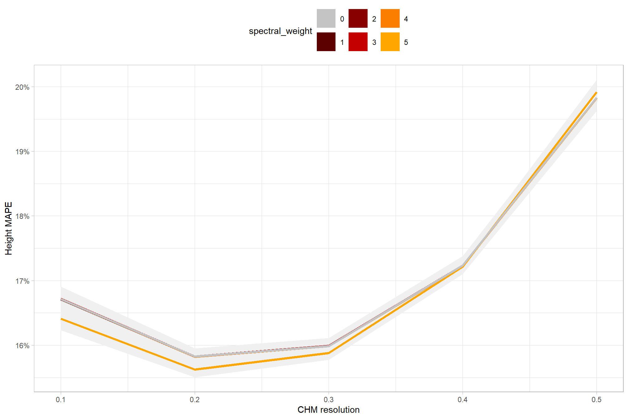
this trend demonstrates that increasing the coarseness of the CHM data has a minimal impact of about 1 percentage point on Height quantification accuracy for CHM data with resolutions in the range of 0.1m to 0.4m. however, increasing the CHM resolution coarseness beyond this level results in a more significant reduction in Height quantification accuracy (i.e. increase in height MAPE) and height accuracy degrades at an increasing rate the more coarse the CHM data…don’t do it
we can look at the posterior distributions of the expected Height MAPE at different CHM resolution levels by the inclusion (or exclusion) of spectral data and it’s weighting…make sure to note the y-axis range (it’s fairly narrow)
draws_temp %>%
  ggplot2::ggplot(mapping = ggplot2::aes(y=value, x=chm_res_m)) +
  tidybayes::stat_eye(
    mapping = ggplot2::aes(fill = spectral_weight)
    , point_interval = median_hdi, .width = .95
    , slab_alpha = 0.95
    , interval_color = "gray44", linewidth = 1
    , point_color = "gray44", point_fill = "gray44", point_size = 1
  ) +
  ggplot2::facet_grid(cols = dplyr::vars(spectral_weight), labeller = "label_both") +
  ggplot2::scale_fill_manual(values = pal_spectral_weight) +
  ggplot2::scale_y_continuous(limits = c(0,NA), labels = scales::percent, breaks = scales::breaks_extended(16)) +
  ggplot2::labs(x = "CHM resolution", y = "Height MAPE") +
  ggplot2::theme_light() +
  ggplot2::theme(
    legend.position = "none"
    , strip.text = ggplot2::element_text(size = 8, color = "black", face = "bold")
  )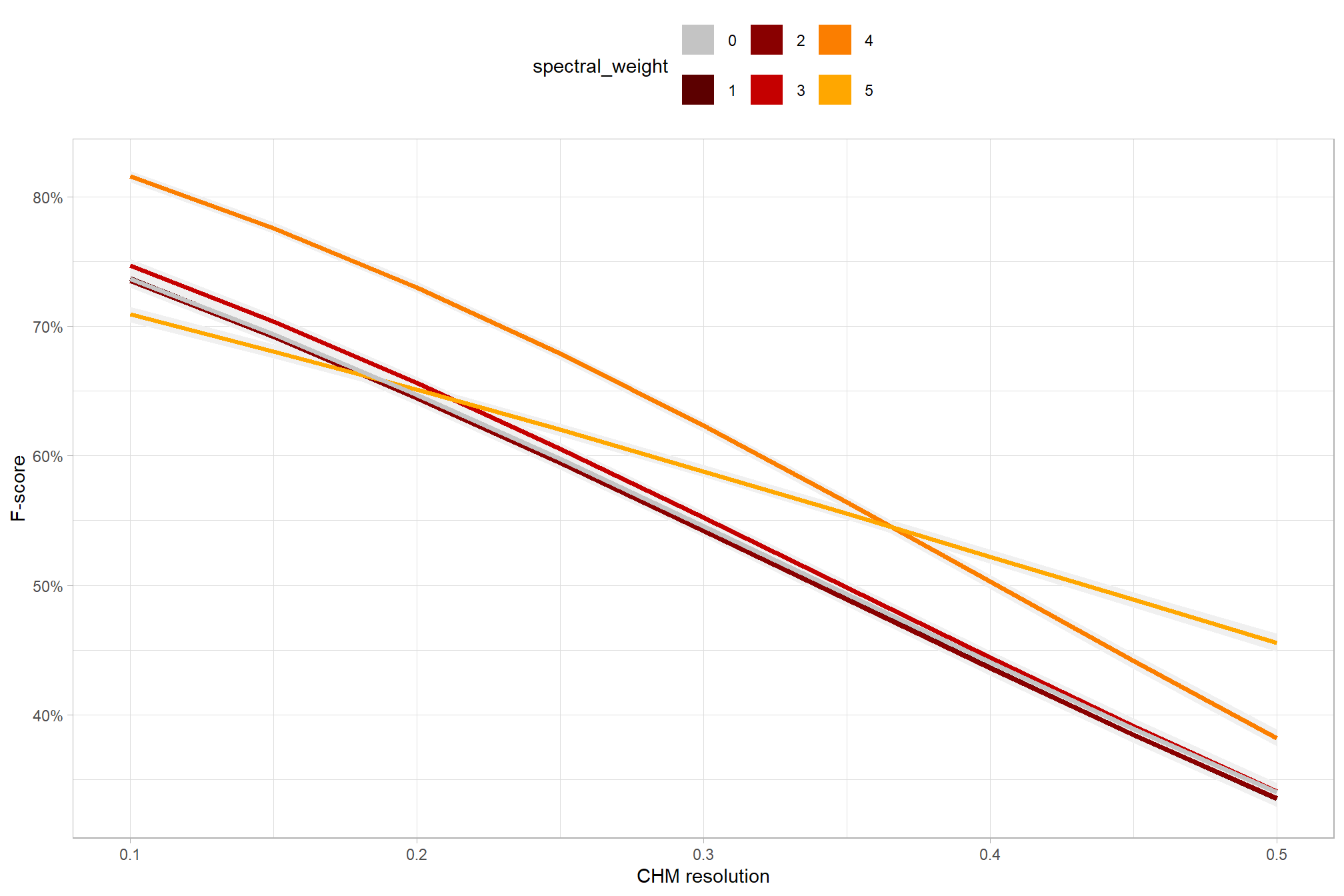
table that
draws_temp %>%
  dplyr::mutate(spectral_weight = forcats::fct_relabel(spectral_weight,~paste0("spectral_weight: ", .x, recycle0 = T))) %>%
  dplyr::group_by(spectral_weight, chm_res_m) %>%
  dplyr::summarise(
    # get median_hdi
    median_hdi_est = tidybayes::median_hdci(value)$y
    , median_hdi_lower = tidybayes::median_hdci(value)$ymin
    , median_hdi_upper = tidybayes::median_hdci(value)$ymax
  ) %>%
  # format pcts
  dplyr::mutate(dplyr::across(
    tidyselect::starts_with("median_hdi_")
    , ~ scales::percent(.x, accuracy = 0.1)
  )) %>%
  dplyr::ungroup() %>%
  dplyr::arrange(spectral_weight, chm_res_m) %>%
  kableExtra::kbl(
    digits = 2
    , caption = "Height MAPE<br>95% HDI of the posterior predictive distribution"
    , col.names = c(
      "spectral_weight", "CHM resolution"
      , c("Height MAPE<br>median", "HDI low", "HDI high")
    )
    , escape = F
  ) %>%
  kableExtra::kable_styling() %>%
  kableExtra::collapse_rows(columns = 1, valign = "top") %>%
kableExtra::scroll_box(height = "8in")| spectral_weight | CHM resolution |
Height MAPE median |
HDI low | HDI high |
|---|---|---|---|---|
| spectral_weight: 0 | 0.1 | 16.7% | 16.5% | 16.9% |
| 0.2 | 15.8% | 15.7% | 15.9% | |
| 0.3 | 16.0% | 15.9% | 16.1% | |
| 0.4 | 17.2% | 17.1% | 17.4% | |
| 0.5 | 19.8% | 19.6% | 20.0% | |
| spectral_weight: 1 | 0.1 | 16.7% | 16.6% | 16.9% |
| 0.2 | 15.8% | 15.7% | 15.9% | |
| 0.3 | 16.0% | 15.9% | 16.1% | |
| 0.4 | 17.2% | 17.1% | 17.4% | |
| 0.5 | 19.8% | 19.6% | 20.0% | |
| spectral_weight: 2 | 0.1 | 16.7% | 16.6% | 16.9% |
| 0.2 | 15.8% | 15.7% | 15.9% | |
| 0.3 | 16.0% | 15.9% | 16.1% | |
| 0.4 | 17.2% | 17.1% | 17.4% | |
| 0.5 | 19.8% | 19.6% | 20.0% | |
| spectral_weight: 3 | 0.1 | 16.7% | 16.6% | 16.9% |
| 0.2 | 15.8% | 15.7% | 16.0% | |
| 0.3 | 16.0% | 15.9% | 16.1% | |
| 0.4 | 17.2% | 17.1% | 17.4% | |
| 0.5 | 19.8% | 19.6% | 20.0% | |
| spectral_weight: 4 | 0.1 | 16.7% | 16.6% | 16.9% |
| 0.2 | 15.8% | 15.7% | 15.9% | |
| 0.3 | 16.0% | 15.9% | 16.1% | |
| 0.4 | 17.2% | 17.1% | 17.4% | |
| 0.5 | 19.8% | 19.6% | 20.0% | |
| spectral_weight: 5 | 0.1 | 16.4% | 16.2% | 16.6% |
| 0.2 | 15.6% | 15.5% | 15.7% | |
| 0.3 | 15.9% | 15.8% | 16.0% | |
| 0.4 | 17.2% | 17.1% | 17.3% | |
| 0.5 | 19.9% | 19.7% | 20.1% |
note that even though these figures make it seem that height quantification accuracy is much worse for the coarser resolution CHM data compared to the finer resolution data, there is only a ~3 percentage point increase in height MAPE from the finest resolution 0.1m to the coarsest resolution 0.5m tested. for example, when spectral data is not included (i.e. spectral_weight = 0) the predicted Height MAPE is 15.3% using 0.1m CHM data and 18.1% when using 0.5m CHM data.
now we’ll probabilistically test the hypothesis that coarser resolution CHM data results in lower Height quantification accuracy and determine by how much. we’ll look at the influence of CHM resolution based on the inclusion of spectral data (or exclusion) and it’s weighting determined by the spectral_weight parameter
contrast_temp <-
  draws_temp %>%
  dplyr::filter(
    round(chm_res_m,2) == round(chm_res_m,1) # let's just look at every 0.1 m (10 cm)
  ) %>%
  dplyr::group_by(spectral_weight) %>%
  tidybayes::compare_levels(
    value
    , by = chm_res_m
    , comparison =
      # "control"
      # tidybayes::emmeans_comparison("revpairwise")
      "pairwise"
  ) %>%
  # dplyr::glimpse()
  dplyr::rename(contrast = chm_res_m) %>%
  # group the data before calculating contrast variables %>%
  dplyr::group_by(spectral_weight, contrast) %>%
  make_contrast_vars() %>%
  # relabel the label for the facets
  dplyr::mutate(spectral_weight = forcats::fct_relabel(spectral_weight,~paste0("spectral_weight: ", .x, recycle0 = T)))
# huh?
# contrast_temp %>% dplyr::glimpse()

# plot it
plt_contrast(
  contrast_temp
  # , caption_text = form_temp
  , y_axis_title = "CHM resolution contrast"
  , x_axis_title = "difference (Height MAPE)"
  , facet = "spectral_weight"
  , label_size = 0
  , x_expand = c(0.3,0.3)
  , annotate_which = "both"
) +
  labs(
    subtitle = "posterior predictive distribution of group constrasts with 95% & 50% HDI\nby `spectral_weight`"
  )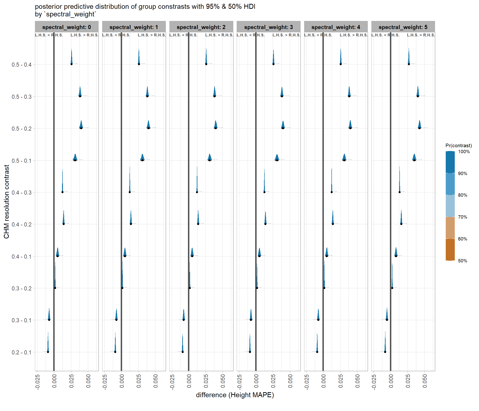
let’s table it
contrast_temp %>%
    dplyr::distinct(
      spectral_weight, contrast
      , median_hdi_est, median_hdi_lower, median_hdi_upper
      , pr_gt_zero # , pr_lt_zero
    ) %>%
    # format pcts
    dplyr::mutate(dplyr::across(
      tidyselect::starts_with("median_hdi_")
      , ~ scales::percent(.x, accuracy = 0.1)
    )) %>%
    dplyr::arrange(spectral_weight, contrast) %>%
    kableExtra::kbl(
      digits = 2
      , caption = "brms::brm model: 95% HDI of the posterior predictive distribution of group constrasts"
      , col.names = c(
        "spectral_weight", "CHM res. contrast"
        , "difference (Height MAPE)"
        , "HDI low", "HDI high"
        , "Pr(diff>0)"
      )
      , escape = F
    ) %>%
    kableExtra::kable_styling() %>%
    kableExtra::collapse_rows(columns = 1, valign = "top") %>%
kableExtra::scroll_box(height = "8in")| spectral_weight | CHM res. contrast | difference (Height MAPE) | HDI low | HDI high | Pr(diff>0) |
|---|---|---|---|---|---|
| spectral_weight: 0 | 0.2 - 0.1 | -0.9% | -1.0% | -0.8% | 0% |
| 0.3 - 0.1 | -0.7% | -0.9% | -0.6% | 0% | |
| 0.3 - 0.2 | 0.2% | 0.1% | 0.2% | 100% | |
| 0.4 - 0.1 | 0.5% | 0.3% | 0.7% | 100% | |
| 0.4 - 0.2 | 1.4% | 1.3% | 1.5% | 100% | |
| 0.4 - 0.3 | 1.3% | 1.2% | 1.3% | 100% | |
| 0.5 - 0.1 | 3.1% | 2.8% | 3.4% | 100% | |
| 0.5 - 0.2 | 4.0% | 3.8% | 4.2% | 100% | |
| 0.5 - 0.3 | 3.8% | 3.7% | 4.0% | 100% | |
| 0.5 - 0.4 | 2.6% | 2.5% | 2.7% | 100% | |
| spectral_weight: 1 | 0.2 - 0.1 | -0.9% | -1.0% | -0.8% | 0% |
| 0.3 - 0.1 | -0.7% | -0.9% | -0.6% | 0% | |
| 0.3 - 0.2 | 0.2% | 0.1% | 0.2% | 100% | |
| 0.4 - 0.1 | 0.5% | 0.3% | 0.7% | 100% | |
| 0.4 - 0.2 | 1.4% | 1.3% | 1.5% | 100% | |
| 0.4 - 0.3 | 1.2% | 1.2% | 1.3% | 100% | |
| 0.5 - 0.1 | 3.1% | 2.8% | 3.4% | 100% | |
| 0.5 - 0.2 | 4.0% | 3.8% | 4.2% | 100% | |
| 0.5 - 0.3 | 3.8% | 3.7% | 4.0% | 100% | |
| 0.5 - 0.4 | 2.6% | 2.5% | 2.7% | 100% | |
| spectral_weight: 2 | 0.2 - 0.1 | -0.9% | -1.0% | -0.8% | 0% |
| 0.3 - 0.1 | -0.7% | -0.9% | -0.6% | 0% | |
| 0.3 - 0.2 | 0.2% | 0.1% | 0.2% | 100% | |
| 0.4 - 0.1 | 0.5% | 0.3% | 0.7% | 100% | |
| 0.4 - 0.2 | 1.4% | 1.3% | 1.5% | 100% | |
| 0.4 - 0.3 | 1.2% | 1.2% | 1.3% | 100% | |
| 0.5 - 0.1 | 3.1% | 2.8% | 3.4% | 100% | |
| 0.5 - 0.2 | 4.0% | 3.8% | 4.2% | 100% | |
| 0.5 - 0.3 | 3.8% | 3.6% | 4.0% | 100% | |
| 0.5 - 0.4 | 2.6% | 2.5% | 2.7% | 100% | |
| spectral_weight: 3 | 0.2 - 0.1 | -0.9% | -1.0% | -0.8% | 0% |
| 0.3 - 0.1 | -0.7% | -0.9% | -0.6% | 0% | |
| 0.3 - 0.2 | 0.2% | 0.1% | 0.2% | 100% | |
| 0.4 - 0.1 | 0.5% | 0.3% | 0.7% | 100% | |
| 0.4 - 0.2 | 1.4% | 1.3% | 1.5% | 100% | |
| 0.4 - 0.3 | 1.2% | 1.2% | 1.3% | 100% | |
| 0.5 - 0.1 | 3.1% | 2.8% | 3.4% | 100% | |
| 0.5 - 0.2 | 4.0% | 3.8% | 4.2% | 100% | |
| 0.5 - 0.3 | 3.8% | 3.7% | 4.0% | 100% | |
| 0.5 - 0.4 | 2.6% | 2.5% | 2.7% | 100% | |
| spectral_weight: 4 | 0.2 - 0.1 | -0.9% | -1.0% | -0.8% | 0% |
| 0.3 - 0.1 | -0.7% | -0.9% | -0.6% | 0% | |
| 0.3 - 0.2 | 0.2% | 0.1% | 0.2% | 100% | |
| 0.4 - 0.1 | 0.5% | 0.3% | 0.7% | 100% | |
| 0.4 - 0.2 | 1.4% | 1.3% | 1.5% | 100% | |
| 0.4 - 0.3 | 1.2% | 1.2% | 1.3% | 100% | |
| 0.5 - 0.1 | 3.1% | 2.8% | 3.4% | 100% | |
| 0.5 - 0.2 | 4.0% | 3.8% | 4.2% | 100% | |
| 0.5 - 0.3 | 3.8% | 3.7% | 4.0% | 100% | |
| 0.5 - 0.4 | 2.6% | 2.5% | 2.7% | 100% | |
| spectral_weight: 5 | 0.2 - 0.1 | -0.8% | -0.9% | -0.7% | 0% |
| 0.3 - 0.1 | -0.5% | -0.7% | -0.4% | 0% | |
| 0.3 - 0.2 | 0.3% | 0.2% | 0.3% | 100% | |
| 0.4 - 0.1 | 0.8% | 0.6% | 1.0% | 100% | |
| 0.4 - 0.2 | 1.6% | 1.5% | 1.7% | 100% | |
| 0.4 - 0.3 | 1.3% | 1.3% | 1.4% | 100% | |
| 0.5 - 0.1 | 3.5% | 3.3% | 3.8% | 100% | |
| 0.5 - 0.2 | 4.3% | 4.1% | 4.5% | 100% | |
| 0.5 - 0.3 | 4.0% | 3.9% | 4.2% | 100% | |
| 0.5 - 0.4 | 2.7% | 2.6% | 2.8% | 100% |
these contrasts confirm what we saw by looking at the predicted relationship between CHM resolution and height MAPE, that increasing the coarseness of the CHM data has a minimal impact of about 1 percentage point on Height quantification accuracy for CHM data with resolutions in the range of 0.1m to 0.4m. however, increasing the CHM resolution coarseness beyond this level results in a more significant reduction in Height quantification accuracy (i.e. increase in height MAPE) and accuracy degrades at an increasing rate the more coarse the CHM data. for example, when spectral data is not included (i.e. spectral_weight = 0) the predicted difference in Height MAPE is ~1% when going from 0.1m to 0.2m-0.4m CHM data but a decrease in height quantification accuracy of ~4 percentage points is predicted going from 0.2m to 0.5m CHM data, for example.
9.3.5.2.2 Spectral data
now we’ll look at the impact of including (or excluding) spectral data and the weighting of the spectral_weight parameter where a value of “0” indicates no spectral data was used (i.e. structural only), the lowest weighting of the spectral data is “1” (only one spectral index threshold must be met), and the highest weighting of spectral data is “5” (all spectral index thresholds must be met).
Note: we expect that the spectral data does not significantly alter the quantification of slash pile form. this is because spectral information is used solely to filter candidate piles, meaning it neither reshapes existing ones nor introduces new detections.
# viridis::rocket(5, begin = 0.9, end = 0.6) %>% scales::show_col()
# brms::posterior_summary(brms_height_mape_mod)
draws_temp %>%
  dplyr::filter(
    round(chm_res_m,2) == round(chm_res_m,1) # let's just look at every 0.1 m (10 cm)
  ) %>%
  ggplot2::ggplot(mapping = ggplot2::aes(x = spectral_weight, y = value, color = factor(chm_res_m))) +
  # tidybayes::stat_halfeye() +
  tidybayes::stat_lineribbon(point_interval = "median_hdi", .width = c(0.95)) +
  # ggplot2::facet_wrap(facets = dplyr::vars(spectral_weight))
  ggplot2::scale_fill_brewer(palette = "Greys") +
  ggplot2::scale_color_viridis_d(option = "rocket", begin = 0.9, end = 0.6) +
  ggplot2::scale_y_continuous(labels = scales::percent) +
  ggplot2::labs(x = "`spectral_weight`", color = "CHM resolution", y = "Height MAPE") +
  ggplot2::theme_light() +
  ggplot2::theme(
    legend.position = "top"
  ) +
  ggplot2::guides(
    color = ggplot2::guide_legend(override.aes = list(shape = 15, lwd = 8, fill = NA))
    , fill = "none"
  )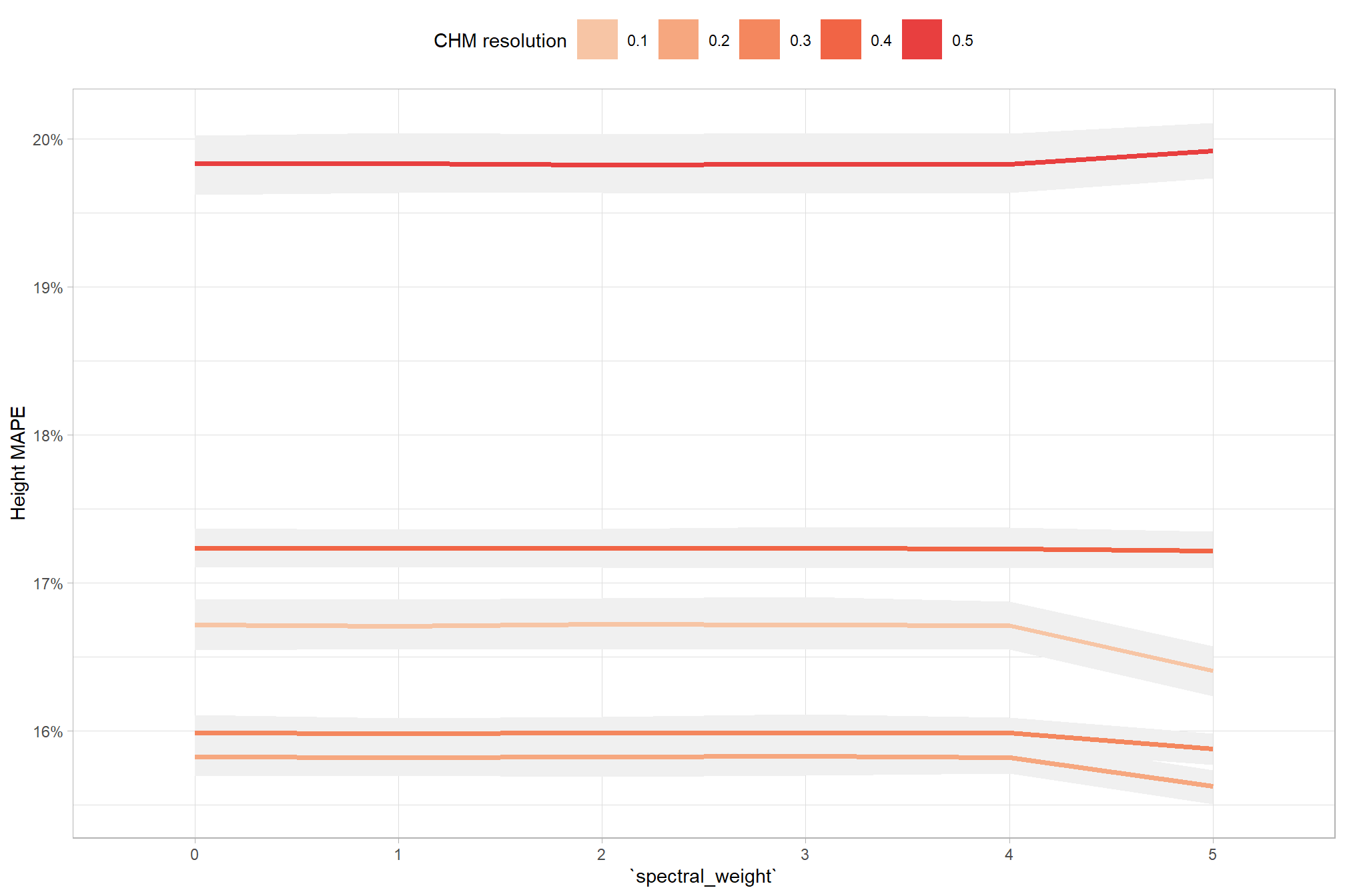
while there is a slight change in height quantification accuracy at the highest spectral weighting, the inclusion of spectral data and the setting of the spectral_weight parameter does not significantly alter the height quantification accuracy irrespective of the CHM resolution
we can look at the posterior distributions of the expected Height MAPE at different spectral_weight settings by the input CHM resolution
draws_temp %>%
  dplyr::filter(
    round(chm_res_m,2) == round(chm_res_m,1) # let's just look at every 0.1 m (10 cm)
  ) %>%
  dplyr::mutate(chm_res_m = chm_res_m %>% factor() %>% forcats::fct_relabel(~paste0("CHM resolution: ", .x, recycle0 = T))) %>%
  ggplot2::ggplot(mapping = ggplot2::aes(y=value, x=spectral_weight)) +
  tidybayes::stat_eye(
    mapping = ggplot2::aes(fill = chm_res_m)
    , point_interval = median_hdi, .width = .95
    , slab_alpha = 0.95
    , interval_color = "gray44", linewidth = 1
    , point_color = "gray44", point_fill = "gray44", point_size = 1
  ) +
  ggplot2::facet_grid(cols = dplyr::vars(chm_res_m)) +
  ggplot2::scale_fill_viridis_d(option = "rocket", begin = 0.9, end = 0.6) +
  ggplot2::scale_y_continuous(limits = c(0,NA), labels = scales::percent, breaks = scales::breaks_extended(16)) +
  ggplot2::labs(x = "`spectral_weight`", y = "Height MAPE") +
  ggplot2::theme_light() +
  ggplot2::theme(
    legend.position = "none"
    , strip.text = ggplot2::element_text(size = 8, color = "black", face = "bold")
  )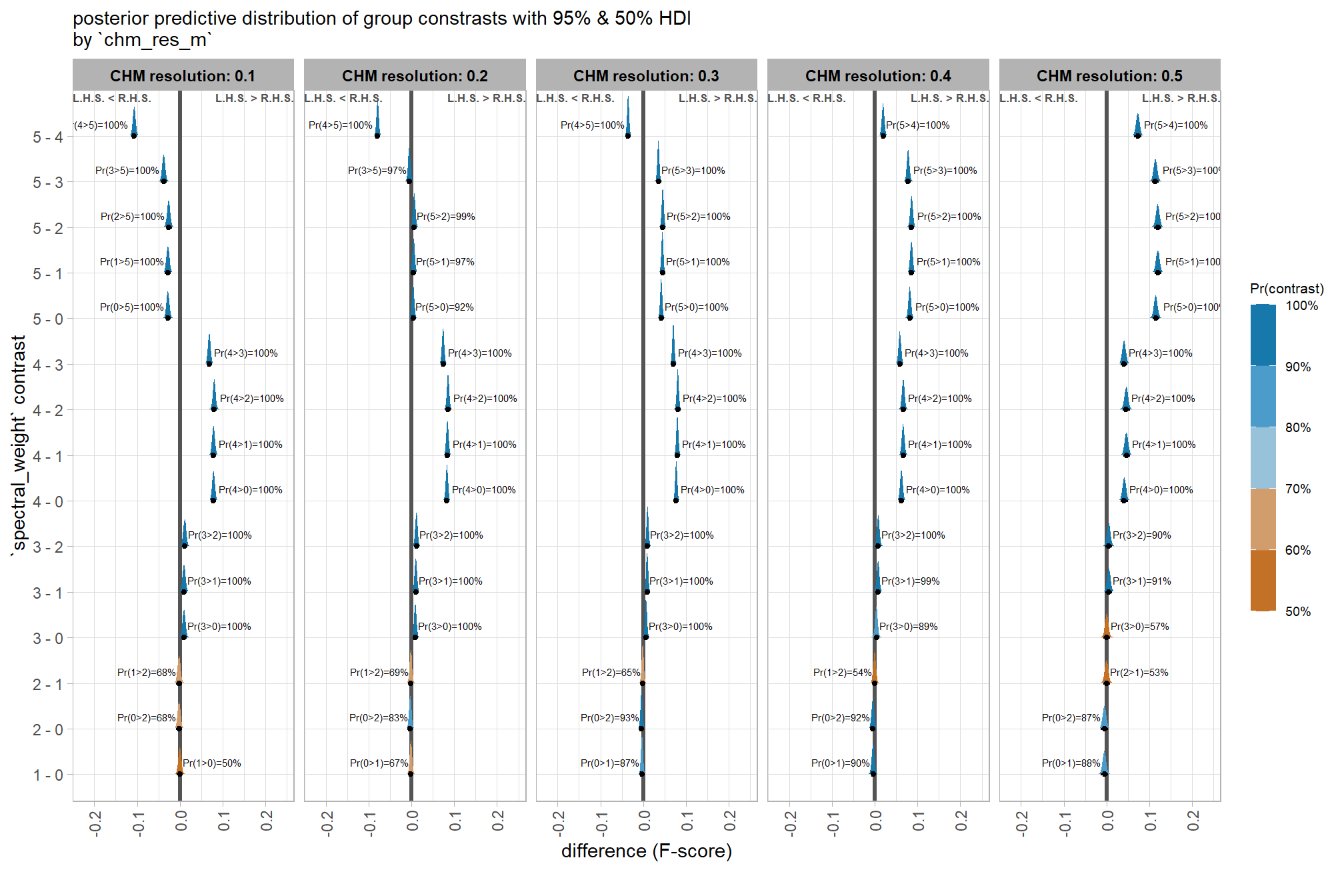
we already saw this same data above in our CHM resolution testing, but we’ll table that again but this time grouping by CHM resolution
draws_temp %>%
  dplyr::filter(
    round(chm_res_m,2) == round(chm_res_m,1) # let's just look at every 0.1 m (10 cm)
  ) %>%
  dplyr::mutate(chm_res_m = chm_res_m %>% factor() %>% forcats::fct_relabel(~paste0("CHM resolution: ", .x, recycle0 = T))) %>%
  dplyr::group_by(chm_res_m, spectral_weight) %>%
  dplyr::summarise(
    # get median_hdi
    median_hdi_est = tidybayes::median_hdci(value)$y
    , median_hdi_lower = tidybayes::median_hdci(value)$ymin
    , median_hdi_upper = tidybayes::median_hdci(value)$ymax
  ) %>%
  # format pcts
  dplyr::mutate(dplyr::across(
    tidyselect::starts_with("median_hdi_")
    , ~ scales::percent(.x, accuracy = 0.1)
  )) %>%
  dplyr::ungroup() %>%
  dplyr::arrange(chm_res_m,spectral_weight) %>%
  kableExtra::kbl(
    digits = 2
    , caption = "Height MAPE<br>95% HDI of the posterior predictive distribution"
    , col.names = c(
      "CHM resolution", "spectral_weight"
      , c("Height MAPE<br>median", "HDI low", "HDI high")
    )
    , escape = F
  ) %>%
  kableExtra::kable_styling() %>%
  kableExtra::collapse_rows(columns = 1, valign = "top") %>%
kableExtra::scroll_box(height = "8in")| CHM resolution | spectral_weight |
Height MAPE median |
HDI low | HDI high |
|---|---|---|---|---|
| CHM resolution: 0.1 | 0 | 16.7% | 16.5% | 16.9% |
| 1 | 16.7% | 16.6% | 16.9% | |
| 2 | 16.7% | 16.6% | 16.9% | |
| 3 | 16.7% | 16.6% | 16.9% | |
| 4 | 16.7% | 16.6% | 16.9% | |
| 5 | 16.4% | 16.2% | 16.6% | |
| CHM resolution: 0.2 | 0 | 15.8% | 15.7% | 15.9% |
| 1 | 15.8% | 15.7% | 15.9% | |
| 2 | 15.8% | 15.7% | 15.9% | |
| 3 | 15.8% | 15.7% | 16.0% | |
| 4 | 15.8% | 15.7% | 15.9% | |
| 5 | 15.6% | 15.5% | 15.7% | |
| CHM resolution: 0.3 | 0 | 16.0% | 15.9% | 16.1% |
| 1 | 16.0% | 15.9% | 16.1% | |
| 2 | 16.0% | 15.9% | 16.1% | |
| 3 | 16.0% | 15.9% | 16.1% | |
| 4 | 16.0% | 15.9% | 16.1% | |
| 5 | 15.9% | 15.8% | 16.0% | |
| CHM resolution: 0.4 | 0 | 17.2% | 17.1% | 17.4% |
| 1 | 17.2% | 17.1% | 17.4% | |
| 2 | 17.2% | 17.1% | 17.4% | |
| 3 | 17.2% | 17.1% | 17.4% | |
| 4 | 17.2% | 17.1% | 17.4% | |
| 5 | 17.2% | 17.1% | 17.3% | |
| CHM resolution: 0.5 | 0 | 19.8% | 19.6% | 20.0% |
| 1 | 19.8% | 19.6% | 20.0% | |
| 2 | 19.8% | 19.6% | 20.0% | |
| 3 | 19.8% | 19.6% | 20.0% | |
| 4 | 19.8% | 19.6% | 20.0% | |
| 5 | 19.9% | 19.7% | 20.1% |
now we’ll probabilistically test the hypothesis that the inclusion of spectral data improves detection accuracy and quantify by how much. we’ll look at the influence of spectral data based on the CHM resolution
to actually compare the different levels of spectral_weight, we’ll use the MCMC draws to contrast the posterior predictions at different levels of the parameter (see below)
contrast_temp <-
  draws_temp %>%
  dplyr::filter(
    round(chm_res_m,2) == round(chm_res_m,1) # let's just look at every 0.1 m (10 cm)
  ) %>%
  dplyr::group_by(chm_res_m) %>%
  tidybayes::compare_levels(
    value
    , by = spectral_weight
    , comparison =
      # tidybayes::emmeans_comparison("revpairwise")
      "pairwise"
  ) %>%
  # dplyr::glimpse()
  dplyr::rename(contrast = spectral_weight) %>%
  # group the data before calculating contrast variables %>%
  dplyr::group_by(chm_res_m, contrast) %>%
  make_contrast_vars() %>%
  # relabel the label for the facets
  dplyr::mutate(chm_res_m = chm_res_m %>% factor() %>% forcats::fct_relabel(~paste0("CHM resolution: ", .x, recycle0 = T)))
# huh?
# contrast_temp %>% dplyr::glimpse()

# plot it
plt_contrast(
  contrast_temp
  # , caption_text = form_temp
  , y_axis_title = "`spectral_weight` contrast"
  , x_axis_title = "difference (Height MAPE)"
  , facet = "chm_res_m"
  , label_size = 1.7
  , x_expand = c(0.4,0.3)
) +
  labs(
    subtitle = "posterior predictive distribution of group constrasts with 95% & 50% HDI\nby `chm_res_m`"
  )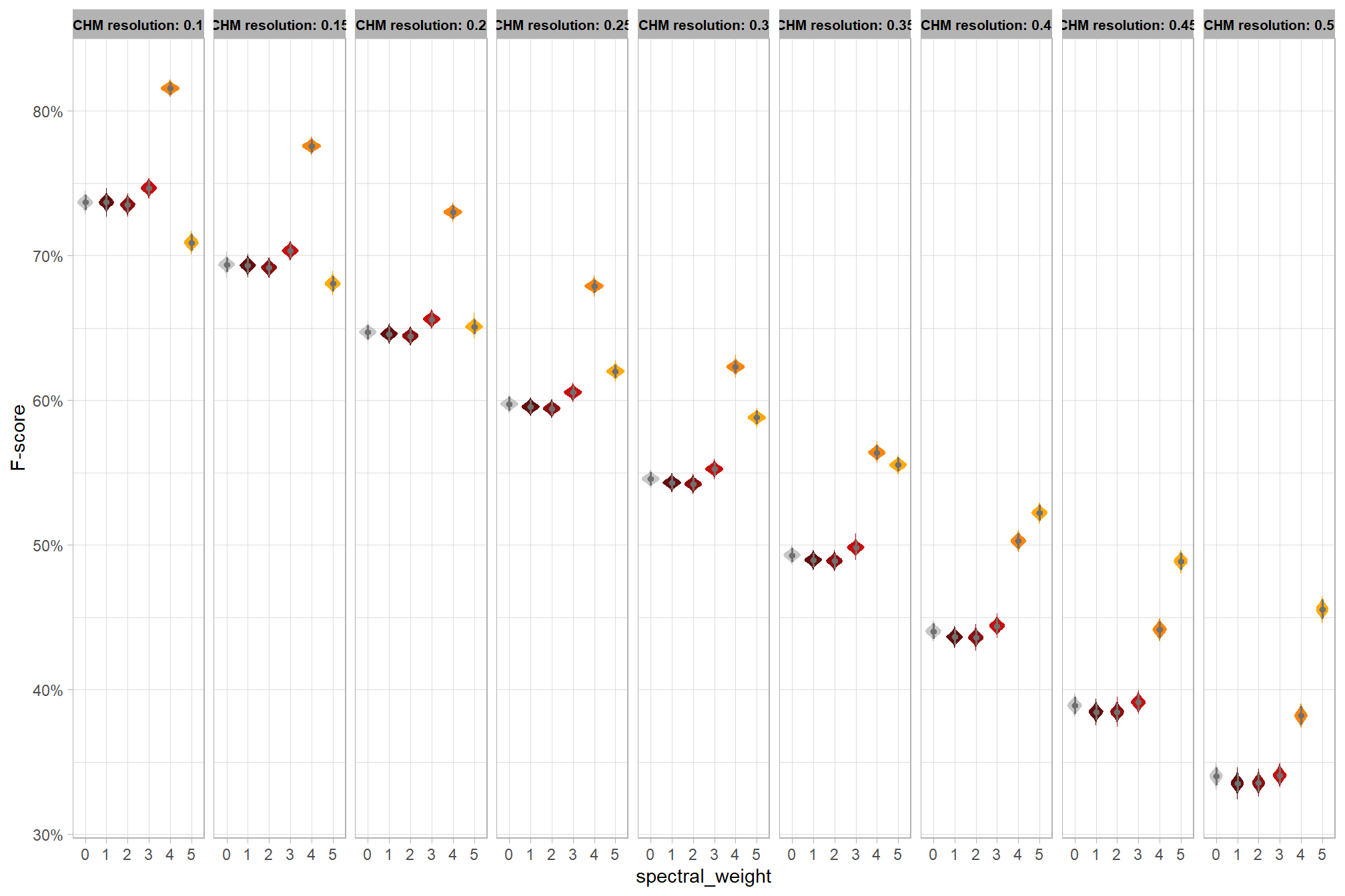
let’s table it
contrast_temp %>%
    dplyr::distinct(
      chm_res_m, contrast
      , median_hdi_est, median_hdi_lower, median_hdi_upper
      # , pr_lt_zero
      , pr_gt_zero
    ) %>%
    dplyr::arrange(chm_res_m, contrast) %>%
    # format pcts
    dplyr::mutate(dplyr::across(
      tidyselect::starts_with("median_hdi_")
      , ~ scales::percent(.x, accuracy = 0.1)
    )) %>%
    kableExtra::kbl(
      digits = 2
      , caption = "brms::brm model: 95% HDI of the posterior predictive distribution of group constrasts"
      , col.names = c(
        "CHM resolution", "spectral_weight"
        , "difference (Height MAPE)"
        , "HDI low", "HDI high"
        # , "Pr(diff<0)"
        , "Pr(diff>0)"
      )
      , escape = F
    ) %>%
    kableExtra::kable_styling() %>%
    kableExtra::collapse_rows(columns = 1, valign = "top") %>%
kableExtra::scroll_box(height = "8in")| CHM resolution | spectral_weight | difference (Height MAPE) | HDI low | HDI high | Pr(diff>0) |
|---|---|---|---|---|---|
| CHM resolution: 0.1 | 1 - 0 | 0.0% | -0.2% | 0.3% | 50% |
| 2 - 0 | 0.0% | -0.2% | 0.2% | 51% | |
| 2 - 1 | 0.0% | -0.2% | 0.2% | 52% | |
| 3 - 0 | 0.0% | -0.2% | 0.2% | 51% | |
| 3 - 1 | 0.0% | -0.2% | 0.2% | 53% | |
| 3 - 2 | 0.0% | -0.2% | 0.2% | 50% | |
| 4 - 0 | 0.0% | -0.2% | 0.2% | 50% | |
| 4 - 1 | 0.0% | -0.2% | 0.2% | 51% | |
| 4 - 2 | 0.0% | -0.2% | 0.2% | 49% | |
| 4 - 3 | 0.0% | -0.2% | 0.2% | 48% | |
| 5 - 0 | -0.3% | -0.5% | -0.1% | 0% | |
| 5 - 1 | -0.3% | -0.5% | -0.1% | 0% | |
| 5 - 2 | -0.3% | -0.5% | -0.1% | 0% | |
| 5 - 3 | -0.3% | -0.5% | -0.1% | 0% | |
| 5 - 4 | -0.3% | -0.5% | -0.1% | 0% | |
| CHM resolution: 0.2 | 1 - 0 | 0.0% | -0.1% | 0.2% | 50% |
| 2 - 0 | 0.0% | -0.1% | 0.1% | 50% | |
| 2 - 1 | 0.0% | -0.1% | 0.1% | 50% | |
| 3 - 0 | 0.0% | -0.1% | 0.1% | 51% | |
| 3 - 1 | 0.0% | -0.1% | 0.1% | 53% | |
| 3 - 2 | 0.0% | -0.1% | 0.1% | 50% | |
| 4 - 0 | 0.0% | -0.1% | 0.1% | 50% | |
| 4 - 1 | 0.0% | -0.1% | 0.1% | 50% | |
| 4 - 2 | 0.0% | -0.1% | 0.1% | 49% | |
| 4 - 3 | 0.0% | -0.1% | 0.1% | 47% | |
| 5 - 0 | -0.2% | -0.3% | -0.1% | 0% | |
| 5 - 1 | -0.2% | -0.3% | -0.1% | 0% | |
| 5 - 2 | -0.2% | -0.3% | -0.1% | 1% | |
| 5 - 3 | -0.2% | -0.3% | -0.1% | 0% | |
| 5 - 4 | -0.2% | -0.3% | -0.1% | 0% | |
| CHM resolution: 0.3 | 1 - 0 | 0.0% | -0.1% | 0.1% | 50% |
| 2 - 0 | 0.0% | -0.1% | 0.1% | 51% | |
| 2 - 1 | 0.0% | -0.1% | 0.1% | 52% | |
| 3 - 0 | 0.0% | -0.1% | 0.1% | 52% | |
| 3 - 1 | 0.0% | -0.1% | 0.1% | 52% | |
| 3 - 2 | 0.0% | -0.1% | 0.1% | 51% | |
| 4 - 0 | 0.0% | -0.1% | 0.1% | 49% | |
| 4 - 1 | 0.0% | -0.1% | 0.1% | 50% | |
| 4 - 2 | 0.0% | -0.1% | 0.1% | 50% | |
| 4 - 3 | 0.0% | -0.1% | 0.1% | 47% | |
| 5 - 0 | -0.1% | -0.2% | 0.0% | 3% | |
| 5 - 1 | -0.1% | -0.2% | 0.0% | 3% | |
| 5 - 2 | -0.1% | -0.2% | 0.0% | 2% | |
| 5 - 3 | -0.1% | -0.2% | 0.0% | 2% | |
| 5 - 4 | -0.1% | -0.2% | 0.0% | 2% | |
| CHM resolution: 0.4 | 1 - 0 | 0.0% | -0.1% | 0.2% | 50% |
| 2 - 0 | 0.0% | -0.2% | 0.1% | 49% | |
| 2 - 1 | 0.0% | -0.2% | 0.1% | 50% | |
| 3 - 0 | 0.0% | -0.1% | 0.2% | 49% | |
| 3 - 1 | 0.0% | -0.2% | 0.1% | 50% | |
| 3 - 2 | 0.0% | -0.1% | 0.2% | 50% | |
| 4 - 0 | 0.0% | -0.2% | 0.1% | 49% | |
| 4 - 1 | 0.0% | -0.1% | 0.1% | 49% | |
| 4 - 2 | 0.0% | -0.1% | 0.1% | 51% | |
| 4 - 3 | 0.0% | -0.2% | 0.1% | 50% | |
| 5 - 0 | 0.0% | -0.2% | 0.1% | 41% | |
| 5 - 1 | 0.0% | -0.2% | 0.1% | 39% | |
| 5 - 2 | 0.0% | -0.2% | 0.1% | 41% | |
| 5 - 3 | 0.0% | -0.2% | 0.1% | 40% | |
| 5 - 4 | 0.0% | -0.2% | 0.1% | 40% | |
| CHM resolution: 0.5 | 1 - 0 | 0.0% | -0.2% | 0.3% | 49% |
| 2 - 0 | 0.0% | -0.3% | 0.2% | 50% | |
| 2 - 1 | 0.0% | -0.2% | 0.2% | 50% | |
| 3 - 0 | 0.0% | -0.3% | 0.2% | 49% | |
| 3 - 1 | 0.0% | -0.2% | 0.3% | 50% | |
| 3 - 2 | 0.0% | -0.2% | 0.3% | 48% | |
| 4 - 0 | 0.0% | -0.3% | 0.2% | 49% | |
| 4 - 1 | 0.0% | -0.2% | 0.3% | 49% | |
| 4 - 2 | 0.0% | -0.2% | 0.2% | 50% | |
| 4 - 3 | 0.0% | -0.3% | 0.2% | 51% | |
| 5 - 0 | 0.1% | -0.2% | 0.3% | 76% | |
| 5 - 1 | 0.1% | -0.1% | 0.3% | 77% | |
| 5 - 2 | 0.1% | -0.2% | 0.3% | 77% | |
| 5 - 3 | 0.1% | -0.2% | 0.3% | 76% | |
| 5 - 4 | 0.1% | -0.2% | 0.3% | 76% |
although we can be very certain that there are differences in Height quantification accuracy (>99% probability across most CHM resolutions) when the spectral_weight is set to “5” (i.e. requiring that all spectral criteria be met) compared to the other settings of spectral_weight or not including spectral data for the finer resolution CHM data (e.g. <0.4m), these differences are so small with nearly all of them showing a difference in Height MAPE of <1%
9.4 Balanced Accuracy Bayesian Optimization
now we’re going to find the optimal parameter settings for our pile detection methodology by using the Bayesian models we developed for F-score (brms_f_score_mod) and MAPE for height (brms_height_mape_mod) and diameter (brms_diam_mape_mod). we’ll use tidybayes::add_epred_draws() to obtain the posterior predictions of the expected value (e.g. F-score) from each model across a common grid of parameter settings (newdata). the predictions from each model will be joined on the parameter settings and draw number (.draw). then we’ll use a customized ranking filter on each posterior draw to find the parameter combination that best balances detection and quantification accuracy. This approach allows us to weight the accuracies according to specific objectives, such as sacrificing some form quantification accuracy to gain better detection accuracy. this methodology is statistically sound because it accounts for uncertainty by using the full posterior distribution from all models throughout the optimization process. unlike methods that rely on single point estimates (like our initial sensitivity testing), this approach can handle complex, non-linear, and interactive relationships. The final output is not a single optimal solution but a posterior distribution of optimal settings, which quantifies the range of credible parameter values that satisfy the optimization criteria.
first, let’s generate the grid to see how many different parameter combinations we’re testing. note, we hold the max_ht_m (2.3 m) and max_area_m2 (46 m2) parameters constant based on our expectations from the treatment prescription implemented on the ground. if we didn’t do this, we would risk over-fitting the optimization based on the training data used.
# grid of parameter settings for use in each tidybayes::add_epred_draws() call
newdata_temp <- tidyr::crossing(
  param_combos_spectral_ranked %>%
    # dplyr::filter(spectral_weight %in% c("0","4","5")) %>%
    dplyr::distinct(spectral_weight)
  , circle_fit_iou_pct = seq(from = 0, to = 1.0, by = 0.02)
  , convexity_pct = seq(from = 0, to = 1.0, by = 0.02)
  , chm_res_m = seq(from = 0.1, to = 0.5, by = 0.05)
  , max_ht_m = structural_params_settings$max_ht_m # seq(from = 2.1, to = 4.3, length.out = 5)
  , max_area_m2 = structural_params_settings$max_area_m2 # seq(from = 20, to = 55, length.out = 5)
)
# huh?
newdata_temp %>% dplyr::glimpse()
## Rows: 140,454
## Columns: 6
## $ spectral_weight <fct> 0, 0, 0, 0, 0, 0, 0, 0, 0, 0, 0, 0, 0, 0, 0, 0, 0, …
## $ circle_fit_iou_pct <dbl> 0, 0, 0, 0, 0, 0, 0, 0, 0, 0, 0, 0, 0, 0, 0, 0, 0, …
## $ convexity_pct <dbl> 0.00, 0.00, 0.00, 0.00, 0.00, 0.00, 0.00, 0.00, 0.0…
## $ chm_res_m <dbl> 0.10, 0.15, 0.20, 0.25, 0.30, 0.35, 0.40, 0.45, 0.5…
## $ max_ht_m <dbl> 2.3, 2.3, 2.3, 2.3, 2.3, 2.3, 2.3, 2.3, 2.3, 2.3, 2…
## $ max_area_m2 <dbl> 46, 46, 46, 46, 46, 46, 46, 46, 46, 46, 46, 46, 46,…the number of records in our newdata is the number of different parameter combinations we’re testing for each draw. modelling allows us to test so many more possible combinations (4.0 times more here) than getting point estimates as we did with our sensitivity testing!
get the posterior predictions from the detection accuracy model F-score (brms_f_score_mod) and MAPE for height (brms_height_mape_mod) and diameter (brms_diam_mape_mod) for quantification accuracy
# names of variables to join the draws on
join_names_temp <- c(names(newdata_temp), ".draw")
ndraws_temp <- 333
# draws
full_draws_temp <-
  # brms_f_score_mod
  tidybayes::add_epred_draws(newdata = newdata_temp, object = brms_f_score_mod, ndraws = ndraws_temp, value = "f_score") %>%
  # join brms_diam_mape_mod
  dplyr::inner_join(
    tidybayes::add_epred_draws(newdata = newdata_temp, object = brms_diam_mape_mod, ndraws = ndraws_temp, value = "diameter_mape")
    , by = join_names_temp
  ) %>%
  # join brms_height_mape_mod
  dplyr::inner_join(
    tidybayes::add_epred_draws(newdata = newdata_temp, object = brms_height_mape_mod, ndraws = ndraws_temp, value = "height_mape")
    , by = join_names_temp
  ) %>%
  # select
  dplyr::select(dplyr::all_of(
    c(join_names_temp, "f_score", "diameter_mape", "height_mape")
  ))
# huh?
full_draws_temp %>% dplyr::glimpse()
## Rows: 46,771,182
## Columns: 10
## Groups: spectral_weight, circle_fit_iou_pct, convexity_pct, chm_res_m, max_ht_m, max_area_m2 [140,454]
## $ spectral_weight <fct> 0, 0, 0, 0, 0, 0, 0, 0, 0, 0, 0, 0, 0, 0, 0, 0, 0, …
## $ circle_fit_iou_pct <dbl> 0, 0, 0, 0, 0, 0, 0, 0, 0, 0, 0, 0, 0, 0, 0, 0, 0, …
## $ convexity_pct <dbl> 0, 0, 0, 0, 0, 0, 0, 0, 0, 0, 0, 0, 0, 0, 0, 0, 0, …
## $ chm_res_m <dbl> 0.1, 0.1, 0.1, 0.1, 0.1, 0.1, 0.1, 0.1, 0.1, 0.1, 0…
## $ max_ht_m <dbl> 2.3, 2.3, 2.3, 2.3, 2.3, 2.3, 2.3, 2.3, 2.3, 2.3, 2…
## $ max_area_m2 <dbl> 46, 46, 46, 46, 46, 46, 46, 46, 46, 46, 46, 46, 46,…
## $ .draw <int> 1, 2, 3, 4, 5, 6, 7, 8, 9, 10, 11, 12, 13, 14, 15, …
## $ f_score <dbl> 0.6170156, 0.5835475, 0.5902940, 0.6036380, 0.60168…
## $ diameter_mape <dbl> 0.1016914, 0.1031600, 0.1029575, 0.1013529, 0.10385…
## $ height_mape <dbl> 0.1809501, 0.1842020, 0.1868028, 0.1835908, 0.18351…the number of records should be equal to the number of records in our newdata multiplied by the number of draws (ndraws)
## [1] TRUE9.4.1 Balanced Accuracy Selection
now we’ll use a customized ranking filter on each posterior draw to find the parameter combination that best balances detection and quantification accuracy. This approach allows us to weight the accuracies according to specific objectives, such as sacrificing some form quantification accuracy to gain better detection accuracy
# weights need to add to 1
weight_detection_temp <- 0.7
weight_quantification_temp <- 0.3
# rank the draws
best_balanced_accuracy_combos <-
  full_draws_temp %>%
  dplyr::group_by(.draw) %>%
  dplyr::mutate(
    pct_rank_detection = dplyr::percent_rank(f_score)
    , dplyr::across(
      .cols = tidyselect::ends_with("_mape")
      , .fn = ~dplyr::percent_rank(-.x) # -mape so largest gets highest pct rank
      , .names = "{.col}_pct_rank"
    )
  ) %>%
  # average of mapes to get quantification mape average
  dplyr::mutate(
    pct_rank_quantification = (height_mape_pct_rank+diameter_mape_pct_rank)/2
    # apply weights to get balanced_accuracy (0-1) with 1 being best
    , balanced_accuracy = (weight_detection_temp*pct_rank_detection) + (weight_quantification_temp*pct_rank_quantification)
  ) %>%
  # dplyr::filter(.draw==1) %>% dplyr::arrange(desc(balanced_accuracy)) %>% View()
  # for each draw, find the setting that maximizes balanced_accuracy
  dplyr::group_by(.draw) %>%
  dplyr::slice_max(order_by = balanced_accuracy, n = 1, with_ties = FALSE) %>%
  dplyr::ungroup() %>%
  dplyr::select(-tidyselect::starts_with("pct_rank_"), -tidyselect::ends_with("_pct_rank"), -balanced_accuracy)
# add on the structural only data
best_balanced_accuracy_combos <-
  full_draws_temp %>%
  dplyr::filter(spectral_weight=="0") %>%
  dplyr::group_by(.draw) %>%
  dplyr::mutate(
    pct_rank_detection = dplyr::percent_rank(f_score)
    , dplyr::across(
      .cols = tidyselect::ends_with("_mape")
      , .fn = ~dplyr::percent_rank(-.x) # -mape so largest gets highest pct rank
      , .names = "{.col}_pct_rank"
    )
  ) %>%
  # average of mapes to get quantification mape average
  dplyr::mutate(
    pct_rank_quantification = (height_mape_pct_rank+diameter_mape_pct_rank)/2
    # apply weights to get balanced_accuracy (0-1) with 1 being best
    , balanced_accuracy = (weight_detection_temp*pct_rank_detection) + (weight_quantification_temp*pct_rank_quantification)
  ) %>%
  # dplyr::filter(.draw==1) %>% dplyr::arrange(desc(balanced_accuracy)) %>% View()
  # for each draw, find the setting that maximizes balanced_accuracy
  dplyr::group_by(.draw) %>%
  dplyr::slice_max(order_by = balanced_accuracy, n = 1, with_ties = FALSE) %>%
  dplyr::ungroup() %>%
  dplyr::select(-tidyselect::starts_with("pct_rank_"), -tidyselect::ends_with("_pct_rank"), -balanced_accuracy) %>%
  # add on data fusion combos
  dplyr::mutate(method_input_data = 0) %>%
  dplyr::bind_rows(
    best_balanced_accuracy_combos %>% dplyr::mutate(method_input_data = 1)
  ) %>%
  dplyr::mutate(
    method_input_data = factor(method_input_data, levels = 0:1, labels = c("structural only", "structural+spectral"), ordered = T)
  )

# huh?
best_balanced_accuracy_combos %>% dplyr::glimpse()
## Rows: 666
## Columns: 11
## $ spectral_weight <fct> 0, 0, 0, 0, 0, 0, 0, 0, 0, 0, 0, 0, 0, 0, 0, 0, 0, …
## $ circle_fit_iou_pct <dbl> 0.44, 0.44, 0.44, 0.44, 0.44, 0.44, 0.44, 0.44, 0.4…
## $ convexity_pct <dbl> 0.08, 0.10, 0.08, 0.10, 0.06, 0.08, 0.08, 0.10, 0.0…
## $ chm_res_m <dbl> 0.1, 0.1, 0.1, 0.1, 0.1, 0.1, 0.1, 0.1, 0.1, 0.1, 0…
## $ max_ht_m <dbl> 2.3, 2.3, 2.3, 2.3, 2.3, 2.3, 2.3, 2.3, 2.3, 2.3, 2…
## $ max_area_m2 <dbl> 46, 46, 46, 46, 46, 46, 46, 46, 46, 46, 46, 46, 46,…
## $ .draw <int> 1, 2, 3, 4, 5, 6, 7, 8, 9, 10, 11, 12, 13, 14, 15, …
## $ f_score <dbl> 0.8069613, 0.7946836, 0.8002498, 0.7988866, 0.79587…
## $ diameter_mape <dbl> 0.1089178, 0.1095609, 0.1086618, 0.1091353, 0.10854…
## $ height_mape <dbl> 0.1545983, 0.1555827, 0.1558584, 0.1555255, 0.15532…
## $ method_input_data <ord> structural only, structural only, structural only, …the number of records 333 corresponds to the number of draws we got from the posterior predictive distribution, each one selected as the parameter combination that best balanced detection and quantification accuracy from the 140,454 tested for the data fusion approach
this output is not a single optimal solution but a posterior distribution of optimal settings, which quantifies the range of credible parameter values that satisfy the optimization criteria.
we’ll have data for both the structural only method and the data fusion method (i.e. “structural+spectral”)
## # A tibble: 2 × 2
##   method_input_data       n
##   <ord>               <int>
## 1 structural only       333
## 2 structural+spectral   333
we also tested different parameter combinations in the absence of spectral data (i.e. spectral_weight = 0) so that we get optimal settings for cases when we only have structural data to attempt to detect piles from
the number of parameter combinations tested per draw with structural data only is equivalent to the number of combinations tested per draw for the data fusion approach divided by six (for spectral_weight setting “1”-“5” and without spectral data “0”):
full_draws_temp %>%
  dplyr::filter(spectral_weight=="0") %>%
  nrow() %>%
  `/`(ndraws_temp) %>%
  scales::comma(accuracy=1)
## [1] "23,409"pivot to long
# pivot to long
best_balanced_accuracy_combos_long <-
  best_balanced_accuracy_combos %>%
  # get rid of vars we fixed
  dplyr::select(-c(max_ht_m, max_area_m2)) %>%
  dplyr::mutate(
    spectral_weight = spectral_weight %>% as.character() %>% as.numeric()
  ) %>%
  tidyr::pivot_longer(cols = -c(.draw,method_input_data))
let’s get the same data but by different CHM resolution levels tested to represent the optimal setting if CHM resolution is fixed and cannot be selected
# let's get the same data but by different CHM resolution levels tested to represent the optimal setting if CHM resolution is fixed and cannot be selected
# rank the draws
best_balanced_accuracy_combos_chm <-
  full_draws_temp %>%
  dplyr::group_by(.draw, chm_res_m) %>%
  dplyr::mutate(
    pct_rank_detection = dplyr::percent_rank(f_score)
    , dplyr::across(
      .cols = tidyselect::ends_with("_mape")
      , .fn = ~dplyr::percent_rank(-.x) # -mape so largest gets highest pct rank
      , .names = "{.col}_pct_rank"
    )
  ) %>%
  # average of mapes to get quantification mape average
  dplyr::mutate(
    pct_rank_quantification = (height_mape_pct_rank+diameter_mape_pct_rank)/2
    # apply weights to get balanced_accuracy (0-1) with 1 being best
    , balanced_accuracy = (weight_detection_temp*pct_rank_detection) + (weight_quantification_temp*pct_rank_quantification)
  ) %>%
  # dplyr::filter(.draw==1) %>% dplyr::arrange(desc(balanced_accuracy)) %>% View()
  # for each draw, find the setting that maximizes balanced_accuracy
  dplyr::group_by(.draw, chm_res_m) %>%
  dplyr::slice_max(order_by = balanced_accuracy, n = 1, with_ties = FALSE) %>%
  dplyr::ungroup() %>%
  dplyr::select(-tidyselect::starts_with("pct_rank_"), -tidyselect::ends_with("_pct_rank"), -balanced_accuracy)
# add on the structural only data
best_balanced_accuracy_combos_chm <-
  full_draws_temp %>%
  dplyr::filter(spectral_weight=="0") %>%
  dplyr::group_by(.draw, chm_res_m) %>%
  dplyr::mutate(
    pct_rank_detection = dplyr::percent_rank(f_score)
    , dplyr::across(
      .cols = tidyselect::ends_with("_mape")
      , .fn = ~dplyr::percent_rank(-.x) # -mape so largest gets highest pct rank
      , .names = "{.col}_pct_rank"
    )
  ) %>%
  # average of mapes to get quantification mape average
  dplyr::mutate(
    pct_rank_quantification = (height_mape_pct_rank+diameter_mape_pct_rank)/2
    # apply weights to get balanced_accuracy (0-1) with 1 being best
    , balanced_accuracy = (weight_detection_temp*pct_rank_detection) + (weight_quantification_temp*pct_rank_quantification)
  ) %>%
  # dplyr::filter(.draw==1) %>% dplyr::arrange(desc(balanced_accuracy)) %>% View()
  # for each draw, find the setting that maximizes balanced_accuracy
  dplyr::group_by(.draw, chm_res_m) %>%
  dplyr::slice_max(order_by = balanced_accuracy, n = 1, with_ties = FALSE) %>%
  dplyr::ungroup() %>%
  dplyr::select(-tidyselect::starts_with("pct_rank_"), -tidyselect::ends_with("_pct_rank"), -balanced_accuracy) %>%
  # add on data fusion combos
  dplyr::mutate(method_input_data = 0) %>%
  dplyr::bind_rows(
    best_balanced_accuracy_combos_chm %>% dplyr::mutate(method_input_data = 1)
  ) %>%
  dplyr::mutate(
    method_input_data = factor(method_input_data, levels = 0:1, labels = c("structural only", "structural+spectral"), ordered = T)
  )
# huh?
best_balanced_accuracy_combos_chm %>% dplyr::glimpse()
## Rows: 5,994
## Columns: 11
## $ spectral_weight <fct> 0, 0, 0, 0, 0, 0, 0, 0, 0, 0, 0, 0, 0, 0, 0, 0, 0, …
## $ circle_fit_iou_pct <dbl> 0.36, 0.40, 0.40, 0.40, 0.36, 0.34, 0.34, 0.34, 0.3…
## $ convexity_pct <dbl> 0.16, 0.18, 0.22, 0.30, 0.36, 0.44, 0.48, 0.54, 0.5…
## $ chm_res_m <dbl> 0.10, 0.15, 0.20, 0.25, 0.30, 0.35, 0.40, 0.45, 0.5…
## $ max_ht_m <dbl> 2.3, 2.3, 2.3, 2.3, 2.3, 2.3, 2.3, 2.3, 2.3, 2.3, 2…
## $ max_area_m2 <dbl> 46, 46, 46, 46, 46, 46, 46, 46, 46, 46, 46, 46, 46,…
## $ .draw <int> 1, 1, 1, 1, 1, 1, 1, 1, 1, 2, 2, 2, 2, 2, 2, 2, 2, …
## $ f_score <dbl> 0.8348130, 0.7974862, 0.7661282, 0.7378913, 0.71128…
## $ diameter_mape <dbl> 0.1098208, 0.1422830, 0.1800632, 0.2222840, 0.26884…
## $ height_mape <dbl> 0.1602975, 0.1554388, 0.1550191, 0.1568298, 0.15998…
## $ method_input_data <ord> structural only, structural only, structural only, …9.4.2 Overall (across CHM resolution)
these recommendations are for users who can generate a CHM from the original point cloud (e.g. using cloud2trees::cloud2raster()). This is a critical distinction because creating a new CHM at the desired resolution is a fundamentally different process than simply disaggregating an existing, coarser raster.
9.4.2.1 Posterior distribution of optimal settings
let’s check out the posterior distribution of optimal settings for each parameter. remember, it is these parameter settings combined that are expected to yield the best balance between detection and quantification accuracy based on our weighting
note, we distinguish the optimal settings based on the availability of spectral data which determines whether or not we can use a data fusion (i.e. “structural+spectral”) approach
# plot it
best_balanced_accuracy_combos_long %>%
  # filter out accuracy metrics
  dplyr::filter(name!="f_score", !stringr::str_ends(name, "_mape")) %>%
  ggplot2::ggplot(mapping = ggplot2::aes(x = value)) +
  tidybayes::stat_dotsinterval(
    point_interval = "median_hdci", .width = c(0.95)
    , quantiles = 100
    , point_size = 3
  ) +
  ggplot2::facet_grid(
    rows = dplyr::vars(method_input_data)
    , cols = dplyr::vars(name)
    , scales = "free_x"
    , axes = "all_x"
  ) +
  ggplot2::scale_y_continuous(NULL, breaks = NULL) +
  # ggplot2::scale_x_continuous(expand = ggplot2::expansion(mult = 1.2)) +
  ggplot2::labs(
    x=""
    , subtitle = paste0(
     "predicted optimal parameter settings based on both detection and quantification accuracy"
    )
  ) +
  ggplot2::theme_light() +
  ggplot2::theme(
    legend.position = "none"
    , strip.text.x = ggplot2::element_text(size = 9, color = "black", face = "bold")
    , strip.text.y = ggplot2::element_text(size = 11, color = "black", face = "bold")
    , axis.text.x = ggplot2::element_text(size = 8, angle = 90)
  )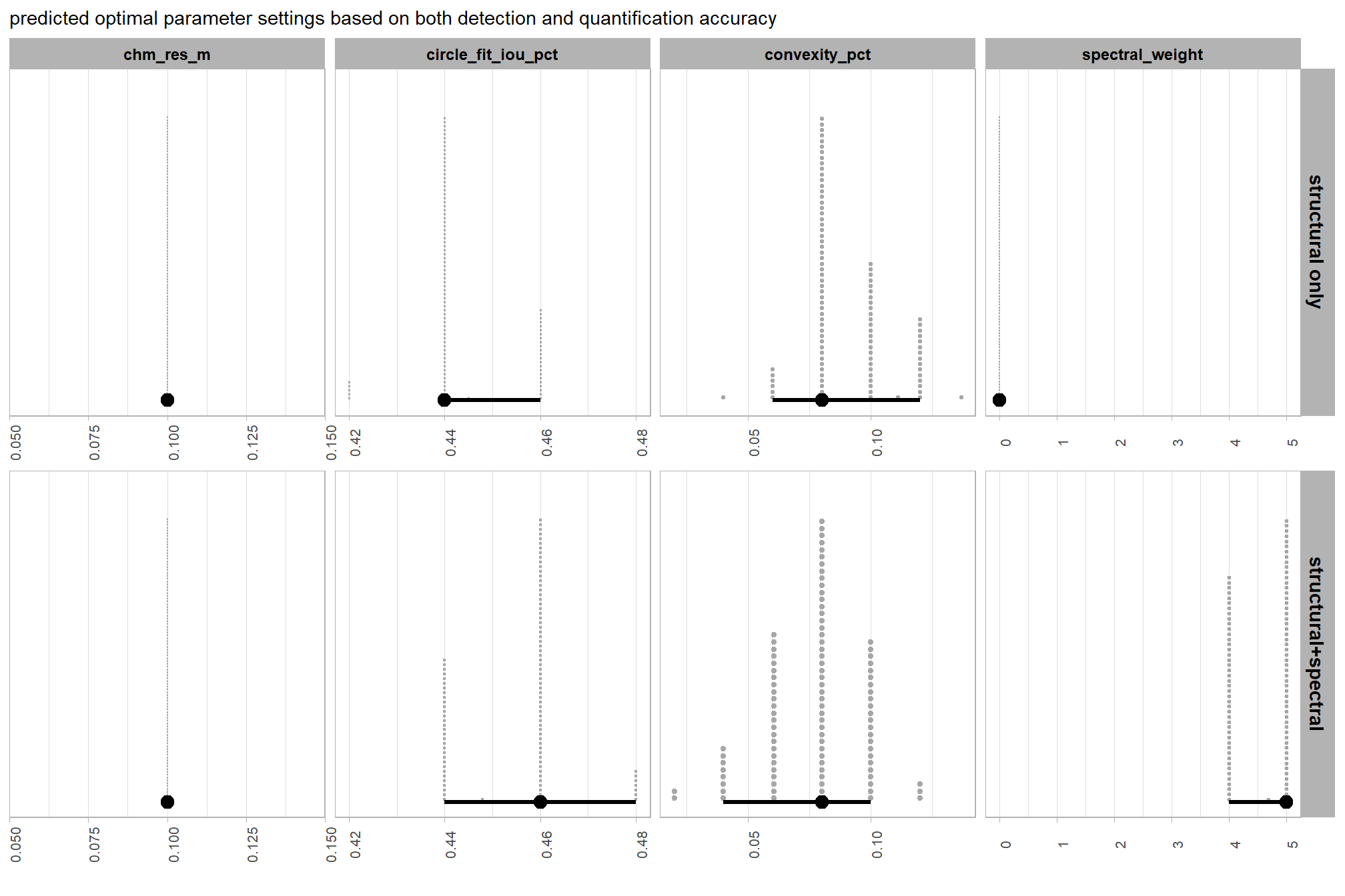
let’s table the HDI of the optimal values
# let's save these optimal settings for later use
# summarize it
optimal_param_settings <- best_balanced_accuracy_combos_long %>%
  # filter out accuracy metrics
  dplyr::filter(name!="f_score", !stringr::str_ends(name, "_mape")) %>%
  dplyr::group_by(method_input_data,name) %>%
  dplyr::summarise(
    # get median_hdi
    median_hdi_est = tidybayes::median_hdci(value)$y
    , median_hdi_lower = tidybayes::median_hdci(value)$ymin
    , median_hdi_upper = tidybayes::median_hdci(value)$ymax
  ) %>%
  dplyr::ungroup()
# table it
optimal_param_settings %>%
  dplyr::mutate(dplyr::across(
    tidyselect::starts_with("median_hdi")
    , ~dplyr::case_when(
      name == "spectral_weight" ~ scales::comma(.x,accuracy=1)
      , T ~scales::comma(.x,accuracy=.01)
    )
  )) %>%
  # table it
  kableExtra::kbl(
    caption = paste0(
     "predicted optimal parameter settings based on both detection and quantification accuracy"
    )
    , col.names = c(
      ".", "parameter"
      , c("median", "HDI low", "HDI high")
    )
    , escape = F
  ) %>%
  kableExtra::kable_styling() %>%
  kableExtra::collapse_rows(columns = 1, valign = "top") %>%
  kableExtra::add_header_above(c(
    " "=2
    , "optimal setting" = 3
))| . | parameter | median | HDI low | HDI high |
|---|---|---|---|---|
| structural only | chm_res_m | 0.10 | 0.10 | 0.10 |
| circle_fit_iou_pct | 0.44 | 0.44 | 0.46 | |
| convexity_pct | 0.08 | 0.06 | 0.12 | |
| spectral_weight | 0 | 0 | 0 | |
| structural+spectral | chm_res_m | 0.10 | 0.10 | 0.10 |
| circle_fit_iou_pct | 0.46 | 0.44 | 0.48 | |
| convexity_pct | 0.08 | 0.04 | 0.10 | |
| spectral_weight | 5 | 4 | 5 |
based on the training data and our model, we have a high degree of certainty that these optimal parameter settings will return the best balanced accuracy. this is evidenced by the 95% highest density intervals (HDIs) of the posterior distribution of optimal solutions, which are either very narrow or centered on a single parameter setting, indicating low uncertainty in the model’s recommendation. However, it is crucial to remember that these settings should be refined based on the actual, on-the-ground treatment prescription and implementation. For example, if a prescription called for piles to be constructed as half-frustum of a cone with rounded ends (lolwut; Hardy 1996), these settings would be inappropriate since they assume mostly circular pile footprints which the method (based on the convexity_pct and circle_fit_iou_pct settings) would not be suited for
9.4.2.2 Posterior distribution of accuracy
what can we expect from a detection and form quantification accuracy perspective?
note, we distinguish the predicted accuracies based on the availability of spectral data which determines whether or not we can use a data fusion (i.e. “structural+spectral”) approach
# plot it
best_balanced_accuracy_combos_long %>%
  dplyr::ungroup() %>%
  # filter for accuracy metrics
  dplyr::filter(name=="f_score" | stringr::str_ends(name, "_mape")) %>%
  dplyr::mutate(
    name = name %>%
      stringr::str_replace_all("_mape", "_MAPE") %>%
      stringr::str_replace_all("f_score", "F-score") %>%
      stringr::str_replace_all("_", " ") %>%
      stringr::str_squish() %>%
      factor(ordered = T) %>%
      forcats::fct_relevel("F-score")
  ) %>%
  ggplot2::ggplot(mapping = ggplot2::aes(x = value)) +
  tidybayes::stat_dotsinterval(
    point_interval = "median_hdci", .width = c(0.95)
    , quantiles = 100
    , point_size = 3
  ) +
  ggplot2::facet_grid(
    rows = dplyr::vars(method_input_data)
    , cols = dplyr::vars(name)
    , scales = "free_x"
    , axes = "all_x"
  ) +
  ggplot2::scale_y_continuous(NULL, breaks = NULL) +
  ggplot2::scale_x_continuous(labels = scales::percent) +
  ggplot2::labs(
    x=""
    , subtitle = paste0(
     "predicted pile detection and form quantification accuracy metrics"
     , "\nusing optimal parameter settings based on both detection and quantification accuracy"
    )
  ) +
  ggplot2::theme_light() +
  ggplot2::theme(
    legend.position = "none"
    , strip.text = ggplot2::element_text(size = 10, color = "black", face = "bold")
    , axis.text.x = ggplot2::element_text(size = 8, angle = 90)
  )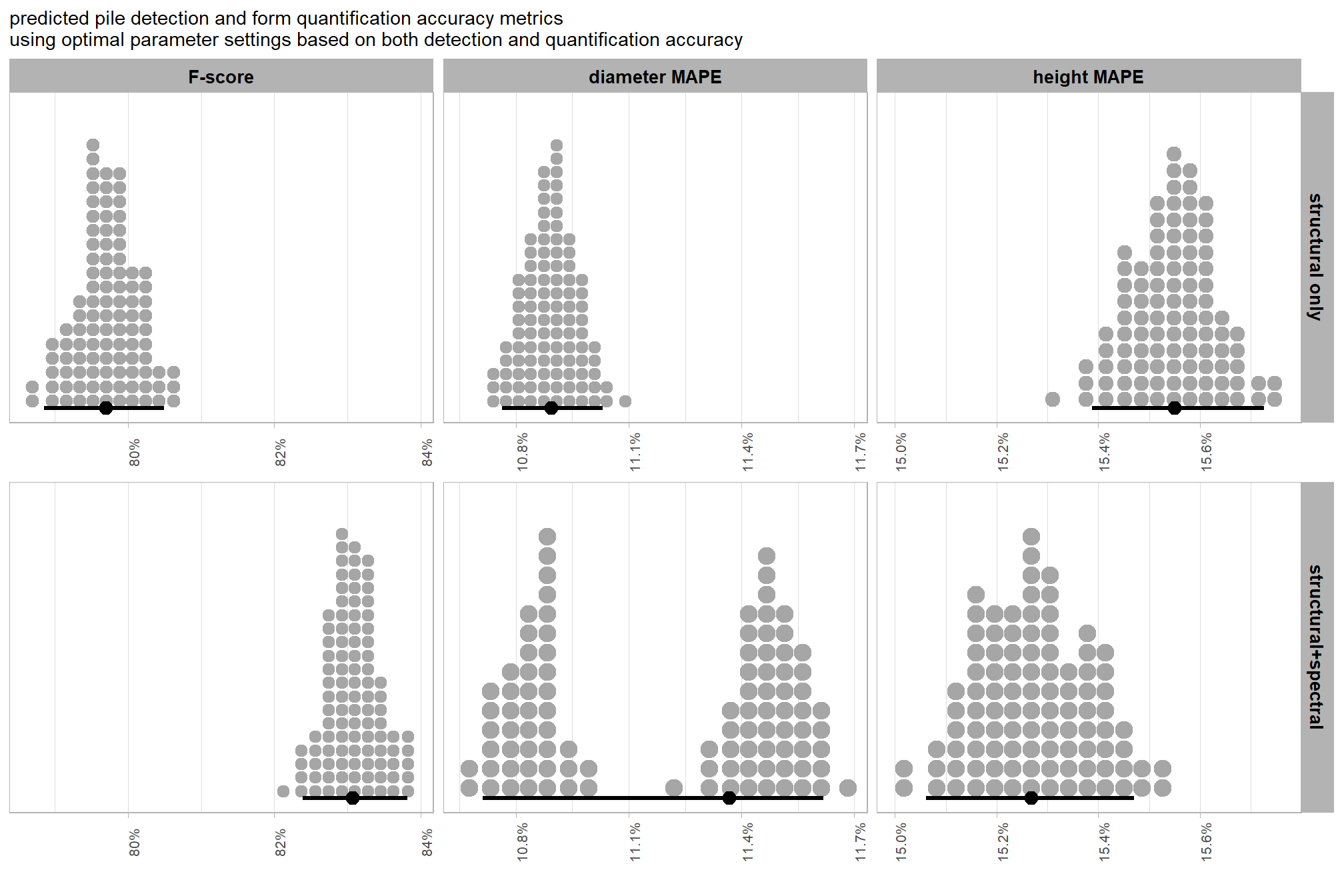
let’s table the HDI of the predicted accuracy metrics
# summarize it
best_balanced_accuracy_combos_long %>%
  dplyr::ungroup() %>%
  # filter for accuracy metrics
  dplyr::filter(name=="f_score" | stringr::str_ends(name, "_mape")) %>%
  dplyr::mutate(
    name = name %>%
      stringr::str_replace_all("_mape", "_MAPE") %>%
      stringr::str_replace_all("f_score", "F-score") %>%
      stringr::str_replace_all("_", " ") %>%
      stringr::str_squish() %>%
      factor(ordered = T) %>%
      forcats::fct_relevel("F-score")
  ) %>%
  dplyr::group_by(method_input_data, name) %>%
  dplyr::summarise(
    # get median_hdi
    median_hdi_est = tidybayes::median_hdci(value)$y
    , median_hdi_lower = tidybayes::median_hdci(value)$ymin
    , median_hdi_upper = tidybayes::median_hdci(value)$ymax
  ) %>%
  dplyr::ungroup() %>%
  dplyr::mutate(dplyr::across(
    tidyselect::starts_with("median_hdi")
    , ~ scales::percent(.x,accuracy=.1)
  )) %>%
  # table it
  kableExtra::kbl(
    caption = paste0(
     "predicted pile detection and form quantification accuracy metrics"
     , "<br>using optimal parameter settings based on both detection and quantification accuracy"
    )
    , col.names = c(
      ".", "metric"
      , c("median", "HDI low", "HDI high")
    )
    , escape = F
  ) %>%
  kableExtra::kable_styling() %>%
  kableExtra::collapse_rows(columns = 1, valign = "top") %>%
  kableExtra::add_header_above(c(
    " "=2
    , "predicted value" = 3
))| . | metric | median | HDI low | HDI high |
|---|---|---|---|---|
| structural only | F-score | 79.7% | 78.9% | 80.5% |
| diameter MAPE | 10.9% | 10.8% | 11.0% | |
| height MAPE | 15.6% | 15.4% | 15.7% | |
| structural+spectral | F-score | 83.1% | 82.4% | 83.8% |
| diameter MAPE | 11.4% | 10.7% | 11.6% | |
| height MAPE | 15.3% | 15.1% | 15.5% |
The narrow 95% highest density intervals (HDIs) of the posterior distribution for the accuracy metrics indicate a high degree of confidence that the method is capable of high detection and form quantification accuracy. This predicted performance, however, is contingent on using the specific optimal parameter settings identified in this analysis. These expectations are specific to the training data, which consisted of piles that were generally circular with few irregularities in their footprint. As such, these results should not be anticipated if the actual on-the-ground pile prescription and implementation differ from those of this training data. Similarly, the same level of accuracy should not be expected if the parameterization of the detection method is altered, even when applied to piles with similar shapes and structures.
9.4.3 by CHM resolution
these recommendations are for users who cannot generate a CHM from the original point cloud and only have access to a CHM at a provided resolution (assuming that resolution is <= 0.5)
# pivot to long
best_balanced_accuracy_combos_long <-
  best_balanced_accuracy_combos_chm %>%
  # get rid of vars we fixed
  dplyr::select(-c(max_ht_m, max_area_m2)) %>%
  dplyr::mutate(
    spectral_weight = spectral_weight %>% as.character() %>% as.numeric()
    , chm_res_m_desc = paste0(chm_res_m, "m CHM") %>% factor() %>% forcats::fct_reorder(chm_res_m)
  ) %>%
  tidyr::pivot_longer(cols = -c(.draw,method_input_data,chm_res_m,chm_res_m_desc))
# best_balanced_accuracy_combos_long %>% dplyr::glimpse()
# best_balanced_accuracy_combos_long %>% dplyr::ungroup() %>% dplyr::count(name)
9.4.3.1 Posterior distribution of optimal settings
let’s check out the posterior distribution of optimal settings for each parameter. remember, it is these parameter settings combined that are expected to yield the best balance between detection and quantification accuracy based on our weighting
9.4.3.1.1 Data Fusion
let’s start with the data fusion approach which assumes users have RGB data to complement the structural CHM data
# plot it
best_balanced_accuracy_combos_long %>%
  dplyr::filter(method_input_data=="structural+spectral") %>%
  # filter out accuracy metrics
  dplyr::filter(name!="f_score", !stringr::str_ends(name, "_mape")) %>%
  ggplot2::ggplot(mapping = ggplot2::aes(x = value)) +
  tidybayes::stat_dotsinterval(
    point_interval = "median_hdci", .width = c(0.95)
    , quantiles = 100
    , point_size = 3
  ) +
  ggplot2::facet_grid(
    rows = dplyr::vars(chm_res_m_desc)
    , cols = dplyr::vars(name)
    , scales = "free_x"
    , axes = "all_x"
  ) +
  ggplot2::scale_y_continuous(NULL, breaks = NULL) +
  # ggplot2::scale_x_continuous(expand = ggplot2::expansion(mult = 1.2)) +
  ggplot2::labs(
    x=""
    , subtitle = paste0(
     "Data Fusion (structural+spectral)"
     , "\npredicted optimal parameter settings based on both detection and quantification accuracy"
    )
  ) +
  ggplot2::theme_light() +
  ggplot2::theme(
    legend.position = "none"
    , strip.text.x = ggplot2::element_text(size = 9, color = "black", face = "bold")
    , strip.text.y = ggplot2::element_text(size = 7, color = "black", face = "bold")
    , axis.text.x = ggplot2::element_text(size = 7, angle = 90)
  )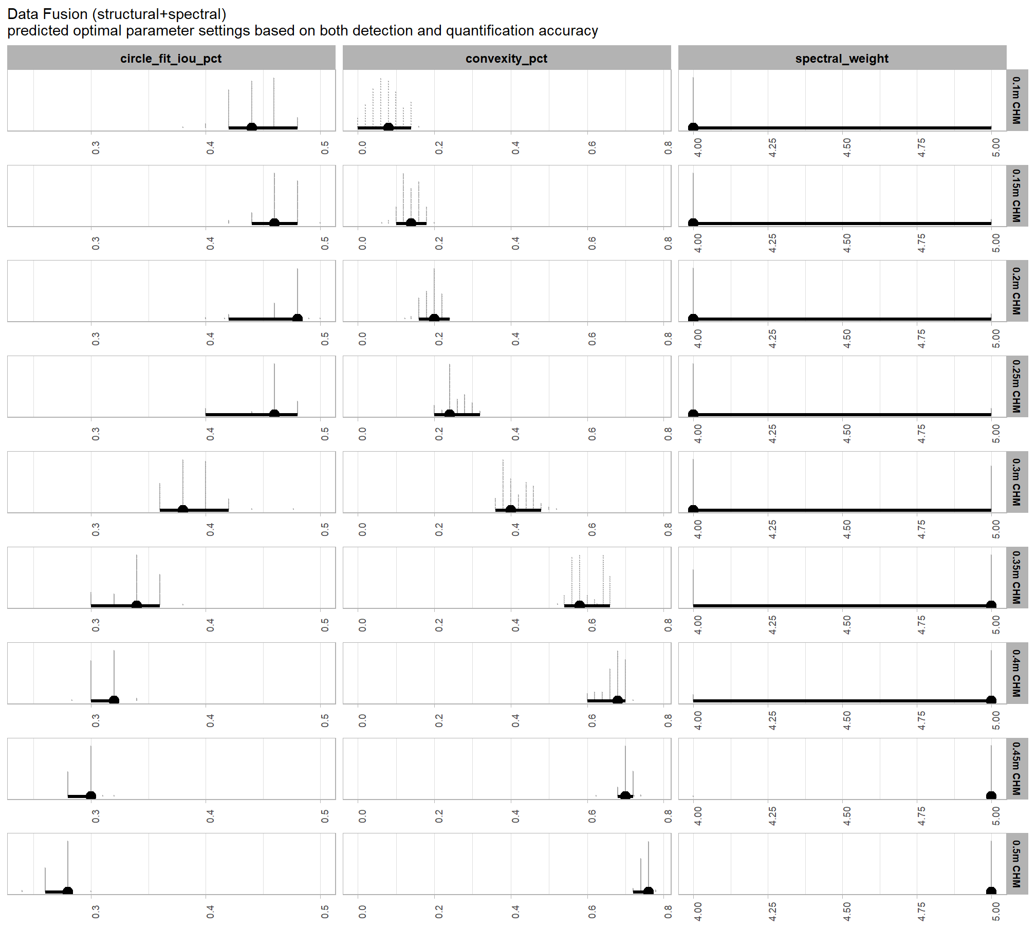
let’s table the HDI of the optimal values
# summarize it
best_balanced_accuracy_combos_long %>%
  dplyr::filter(method_input_data=="structural+spectral") %>%
  # filter out accuracy metrics
  dplyr::filter(name!="f_score", !stringr::str_ends(name, "_mape")) %>%
  dplyr::group_by(chm_res_m_desc,method_input_data,name) %>%
  dplyr::summarise(
    # get median_hdi
    median_hdi_est = tidybayes::median_hdci(value)$y
    , median_hdi_lower = tidybayes::median_hdci(value)$ymin
    , median_hdi_upper = tidybayes::median_hdci(value)$ymax
  ) %>%
  dplyr::ungroup() %>%
  dplyr::mutate(dplyr::across(
    tidyselect::starts_with("median_hdi")
    , ~dplyr::case_when(
      name == "spectral_weight" ~ scales::comma(.x,accuracy=1)
      , T ~scales::comma(.x,accuracy=.01)
    )
  )) %>%
  dplyr::select(-method_input_data) %>%
  # table it
  kableExtra::kbl(
    caption = paste0(
      "Data Fusion (structural+spectral)"
      , "<br>predicted optimal parameter settings based on both detection and quantification accuracy"
    )
    , col.names = c(
      "CHM resolution", "parameter"
      , c("median", "HDI low", "HDI high")
    )
    , escape = F
  ) %>%
  kableExtra::kable_styling() %>%
  kableExtra::collapse_rows(columns = 1, valign = "top") %>%
  kableExtra::add_header_above(c(
    " "=2
    , "optimal setting" = 3
  )) %>%
kableExtra::scroll_box(height = "8in")| CHM resolution | parameter | median | HDI low | HDI high |
|---|---|---|---|---|
| 0.1m CHM | circle_fit_iou_pct | 0.44 | 0.42 | 0.48 |
| convexity_pct | 0.08 | 0.00 | 0.14 | |
| spectral_weight | 4 | 4 | 5 | |
| 0.15m CHM | circle_fit_iou_pct | 0.46 | 0.44 | 0.48 |
| convexity_pct | 0.14 | 0.10 | 0.18 | |
| spectral_weight | 4 | 4 | 5 | |
| 0.2m CHM | circle_fit_iou_pct | 0.48 | 0.42 | 0.48 |
| convexity_pct | 0.20 | 0.16 | 0.24 | |
| spectral_weight | 4 | 4 | 5 | |
| 0.25m CHM | circle_fit_iou_pct | 0.46 | 0.40 | 0.48 |
| convexity_pct | 0.24 | 0.20 | 0.32 | |
| spectral_weight | 4 | 4 | 5 | |
| 0.3m CHM | circle_fit_iou_pct | 0.38 | 0.36 | 0.42 |
| convexity_pct | 0.40 | 0.36 | 0.48 | |
| spectral_weight | 4 | 4 | 5 | |
| 0.35m CHM | circle_fit_iou_pct | 0.34 | 0.30 | 0.36 |
| convexity_pct | 0.58 | 0.54 | 0.66 | |
| spectral_weight | 5 | 4 | 5 | |
| 0.4m CHM | circle_fit_iou_pct | 0.32 | 0.30 | 0.32 |
| convexity_pct | 0.68 | 0.60 | 0.70 | |
| spectral_weight | 5 | 4 | 5 | |
| 0.45m CHM | circle_fit_iou_pct | 0.30 | 0.28 | 0.30 |
| convexity_pct | 0.70 | 0.68 | 0.72 | |
| spectral_weight | 5 | 5 | 5 | |
| 0.5m CHM | circle_fit_iou_pct | 0.28 | 0.26 | 0.28 |
| convexity_pct | 0.76 | 0.72 | 0.76 | |
| spectral_weight | 5 | 5 | 5 |
9.4.3.1.2 Structural only
now we’ll consider an approach that only uses structural data without the benefit of supplemental spectral data
# plot it
best_balanced_accuracy_combos_long %>%
  dplyr::filter(method_input_data=="structural only") %>%
  # filter out accuracy metrics
  dplyr::filter(name!="f_score", !stringr::str_ends(name, "_mape"), name!="spectral_weight") %>%
  ggplot2::ggplot(mapping = ggplot2::aes(x = value)) +
  tidybayes::stat_dotsinterval(
    point_interval = "median_hdci", .width = c(0.95)
    , quantiles = 100
    , point_size = 3
  ) +
  ggplot2::facet_grid(
    rows = dplyr::vars(chm_res_m_desc)
    , cols = dplyr::vars(name)
    , scales = "free_x"
    , axes = "all_x"
  ) +
  ggplot2::scale_y_continuous(NULL, breaks = NULL) +
  # ggplot2::scale_x_continuous(expand = ggplot2::expansion(mult = 1.2)) +
  ggplot2::labs(
    x=""
    , subtitle = paste0(
     "Structural only"
     , "\npredicted optimal parameter settings based on both detection and quantification accuracy"
    )
  ) +
  ggplot2::theme_light() +
  ggplot2::theme(
    legend.position = "none"
    , strip.text.x = ggplot2::element_text(size = 9, color = "black", face = "bold")
    , strip.text.y = ggplot2::element_text(size = 7, color = "black", face = "bold")
    , axis.text.x = ggplot2::element_text(size = 7, angle = 90)
  )
let’s table the HDI of the optimal values
# summarize it
best_balanced_accuracy_combos_long %>%
  dplyr::filter(method_input_data=="structural only") %>%
  # filter out accuracy metrics
  dplyr::filter(name!="f_score", !stringr::str_ends(name, "_mape")) %>%
  dplyr::group_by(chm_res_m_desc,method_input_data,name) %>%
  dplyr::summarise(
    # get median_hdi
    median_hdi_est = tidybayes::median_hdci(value)$y
    , median_hdi_lower = tidybayes::median_hdci(value)$ymin
    , median_hdi_upper = tidybayes::median_hdci(value)$ymax
  ) %>%
  dplyr::ungroup() %>%
  dplyr::mutate(dplyr::across(
    tidyselect::starts_with("median_hdi")
    , ~dplyr::case_when(
      name == "spectral_weight" ~ scales::comma(.x,accuracy=1)
      , T ~scales::comma(.x,accuracy=.01)
    )
  )) %>%
  dplyr::select(-method_input_data) %>%
  # table it
  kableExtra::kbl(
    caption = paste0(
      "Structural only"
      , "<br>predicted optimal parameter settings based on both detection and quantification accuracy"
    )
    , col.names = c(
      "CHM resolution", "parameter"
      , c("median", "HDI low", "HDI high")
    )
    , escape = F
  ) %>%
  kableExtra::kable_styling() %>%
  kableExtra::collapse_rows(columns = 1, valign = "top") %>%
  kableExtra::add_header_above(c(
    " "=2
    , "optimal setting" = 3
  )) %>%
kableExtra::scroll_box(height = "8in")| CHM resolution | parameter | median | HDI low | HDI high |
|---|---|---|---|---|
| 0.1m CHM | circle_fit_iou_pct | 0.38 | 0.36 | 0.38 |
| convexity_pct | 0.16 | 0.14 | 0.18 | |
| spectral_weight | 0 | 0 | 0 | |
| 0.15m CHM | circle_fit_iou_pct | 0.40 | 0.38 | 0.40 |
| convexity_pct | 0.22 | 0.18 | 0.24 | |
| spectral_weight | 0 | 0 | 0 | |
| 0.2m CHM | circle_fit_iou_pct | 0.40 | 0.40 | 0.42 |
| convexity_pct | 0.26 | 0.22 | 0.28 | |
| spectral_weight | 0 | 0 | 0 | |
| 0.25m CHM | circle_fit_iou_pct | 0.40 | 0.40 | 0.42 |
| convexity_pct | 0.30 | 0.30 | 0.32 | |
| spectral_weight | 0 | 0 | 0 | |
| 0.3m CHM | circle_fit_iou_pct | 0.38 | 0.36 | 0.38 |
| convexity_pct | 0.38 | 0.36 | 0.40 | |
| spectral_weight | 0 | 0 | 0 | |
| 0.35m CHM | circle_fit_iou_pct | 0.36 | 0.34 | 0.36 |
| convexity_pct | 0.46 | 0.44 | 0.48 | |
| spectral_weight | 0 | 0 | 0 | |
| 0.4m CHM | circle_fit_iou_pct | 0.34 | 0.34 | 0.36 |
| convexity_pct | 0.48 | 0.48 | 0.50 | |
| spectral_weight | 0 | 0 | 0 | |
| 0.45m CHM | circle_fit_iou_pct | 0.34 | 0.34 | 0.36 |
| convexity_pct | 0.52 | 0.52 | 0.54 | |
| spectral_weight | 0 | 0 | 0 | |
| 0.5m CHM | circle_fit_iou_pct | 0.34 | 0.34 | 0.34 |
| convexity_pct | 0.56 | 0.56 | 0.58 | |
| spectral_weight | 0 | 0 | 0 |
9.4.3.2 Posterior distribution of accuracy
what can we expect from a detection and form quantification accuracy perspective?
9.4.3.2.1 Data Fusion
let’s start with the data fusion approach which assumes users have RGB data to complement the structural CHM data
# plot it
best_balanced_accuracy_combos_long %>%
  dplyr::filter(method_input_data=="structural+spectral") %>%
  # filter out accuracy metrics
  dplyr::filter(name=="f_score" | stringr::str_ends(name, "_mape")) %>%
  dplyr::mutate(
    name = name %>%
      stringr::str_replace_all("_mape", "_MAPE") %>%
      stringr::str_replace_all("f_score", "F-score") %>%
      stringr::str_replace_all("_", " ") %>%
      stringr::str_squish() %>%
      factor(ordered = T) %>%
      forcats::fct_relevel("F-score")
  ) %>%
  ggplot2::ggplot(mapping = ggplot2::aes(x = value)) +
  tidybayes::stat_dotsinterval(
    point_interval = "median_hdci", .width = c(0.95)
    , quantiles = 100
    , point_size = 3
  ) +
  ggplot2::facet_grid(
    rows = dplyr::vars(chm_res_m_desc)
    , cols = dplyr::vars(name)
    , scales = "free_x"
    , axes = "all_x"
  ) +
  ggplot2::scale_y_continuous(NULL, breaks = NULL) +
  ggplot2::scale_x_continuous(labels = scales::percent) +
  ggplot2::labs(
    x=""
    , subtitle = paste0(
     "Data Fusion (structural+spectral)"
     , "\npredicted pile detection and form quantification accuracy metrics"
     , "\nusing optimal parameter settings based on both detection and quantification accuracy"
    )
  ) +
  ggplot2::theme_light() +
  ggplot2::theme(
    legend.position = "none"
    , strip.text.x = ggplot2::element_text(size = 9, color = "black", face = "bold")
    , strip.text.y = ggplot2::element_text(size = 7, color = "black", face = "bold")
    , axis.text.x = ggplot2::element_text(size = 7, angle = 90)
  )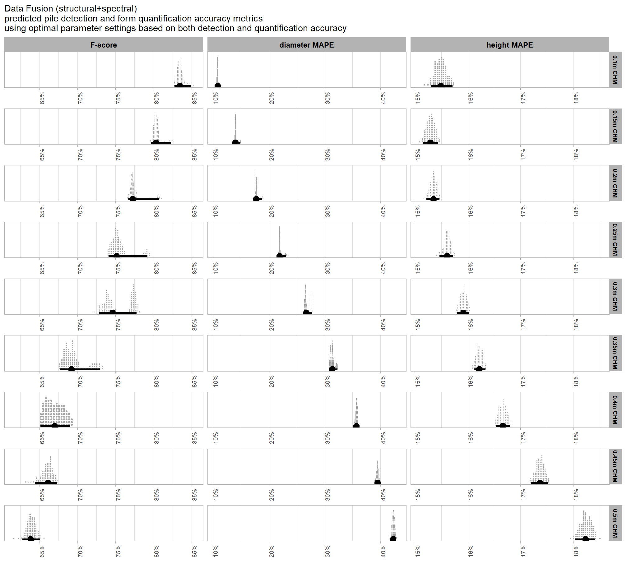
let’s table the HDI of the predicted accuracy metrics
# summarize it
best_balanced_accuracy_combos_long %>%
  dplyr::filter(method_input_data=="structural+spectral") %>%
  dplyr::ungroup() %>%
  # filter for accuracy metrics
  dplyr::filter(name=="f_score" | stringr::str_ends(name, "_mape")) %>%
  dplyr::mutate(
    name = name %>%
      stringr::str_replace_all("_mape", "_MAPE") %>%
      stringr::str_replace_all("f_score", "F-score") %>%
      stringr::str_replace_all("_", " ") %>%
      stringr::str_squish() %>%
      factor(ordered = T) %>%
      forcats::fct_relevel("F-score")
  ) %>%
  dplyr::group_by(chm_res_m_desc, method_input_data, name) %>%
  dplyr::summarise(
    # get median_hdi
    median_hdi_est = tidybayes::median_hdci(value)$y
    , median_hdi_lower = tidybayes::median_hdci(value)$ymin
    , median_hdi_upper = tidybayes::median_hdci(value)$ymax
  ) %>%
  dplyr::ungroup() %>%
  dplyr::mutate(dplyr::across(
    tidyselect::starts_with("median_hdi")
    , ~ scales::percent(.x,accuracy=.1)
  )) %>%
  dplyr::select(-method_input_data) %>%
  # table it
  kableExtra::kbl(
    caption = paste0(
     "Data Fusion (structural+spectral)"
     , "<br>predicted pile detection and form quantification accuracy metrics"
     , "<br>using optimal parameter settings based on both detection and quantification accuracy"
    )
    , col.names = c(
      "CHM Resolution", "metric"
      , c("median", "HDI low", "HDI high")
    )
    , escape = F
  ) %>%
  kableExtra::kable_styling() %>%
  kableExtra::collapse_rows(columns = 1, valign = "top") %>%
  kableExtra::add_header_above(c(
    " "=2
    , "predicted value" = 3
  )) %>%
kableExtra::scroll_box(height = "8in")| CHM Resolution | metric | median | HDI low | HDI high |
|---|---|---|---|---|
| 0.1m CHM | F-score | 83.5% | 82.7% | 84.9% |
| diameter MAPE | 10.9% | 10.7% | 11.2% | |
| height MAPE | 15.5% | 15.3% | 15.7% | |
| 0.15m CHM | F-score | 80.3% | 79.7% | 82.3% |
| diameter MAPE | 14.1% | 13.9% | 15.0% | |
| height MAPE | 15.3% | 15.2% | 15.4% | |
| 0.2m CHM | F-score | 77.3% | 76.6% | 80.7% |
| diameter MAPE | 17.8% | 17.6% | 18.8% | |
| height MAPE | 15.4% | 15.2% | 15.5% | |
| 0.25m CHM | F-score | 75.1% | 74.1% | 79.2% |
| diameter MAPE | 21.9% | 21.7% | 23.1% | |
| height MAPE | 15.6% | 15.5% | 15.7% | |
| 0.3m CHM | F-score | 74.6% | 72.9% | 77.8% |
| diameter MAPE | 26.8% | 26.4% | 27.8% | |
| height MAPE | 15.9% | 15.8% | 16.0% | |
| 0.35m CHM | F-score | 69.2% | 67.7% | 73.0% |
| diameter MAPE | 31.3% | 30.8% | 32.3% | |
| height MAPE | 16.2% | 16.1% | 16.3% | |
| 0.4m CHM | F-score | 67.0% | 65.1% | 69.1% |
| diameter MAPE | 35.7% | 35.2% | 36.0% | |
| height MAPE | 16.7% | 16.5% | 16.8% | |
| 0.45m CHM | F-score | 66.1% | 64.5% | 67.3% |
| diameter MAPE | 39.5% | 39.1% | 39.9% | |
| height MAPE | 17.4% | 17.2% | 17.5% | |
| 0.5m CHM | F-score | 63.9% | 62.8% | 65.1% |
| diameter MAPE | 42.3% | 41.7% | 42.8% | |
| height MAPE | 18.2% | 18.0% | 18.4% |
9.4.3.2.2 Structural only
now we’ll consider an approach that only uses structural data without the benefit of supplemental spectral data
# plot it
best_balanced_accuracy_combos_long %>%
  dplyr::filter(method_input_data=="structural only") %>%
  # filter out accuracy metrics
  dplyr::filter(name=="f_score" | stringr::str_ends(name, "_mape")) %>%
  dplyr::mutate(
    name = name %>%
      stringr::str_replace_all("_mape", "_MAPE") %>%
      stringr::str_replace_all("f_score", "F-score") %>%
      stringr::str_replace_all("_", " ") %>%
      stringr::str_squish() %>%
      factor(ordered = T) %>%
      forcats::fct_relevel("F-score")
  ) %>%
  ggplot2::ggplot(mapping = ggplot2::aes(x = value)) +
  tidybayes::stat_dotsinterval(
    point_interval = "median_hdci", .width = c(0.95)
    , quantiles = 100
    , point_size = 3
  ) +
  ggplot2::facet_grid(
    rows = dplyr::vars(chm_res_m_desc)
    , cols = dplyr::vars(name)
    , scales = "free_x"
    , axes = "all_x"
  ) +
  ggplot2::scale_y_continuous(NULL, breaks = NULL) +
  ggplot2::scale_x_continuous(labels = scales::percent) +
  ggplot2::labs(
    x=""
    , subtitle = paste0(
     "Structural only"
     , "\npredicted pile detection and form quantification accuracy metrics"
     , "\nusing optimal parameter settings based on both detection and quantification accuracy"
    )
  ) +
  ggplot2::theme_light() +
  ggplot2::theme(
    legend.position = "none"
    , strip.text.x = ggplot2::element_text(size = 9, color = "black", face = "bold")
    , strip.text.y = ggplot2::element_text(size = 7, color = "black", face = "bold")
    , axis.text.x = ggplot2::element_text(size = 7, angle = 90)
  )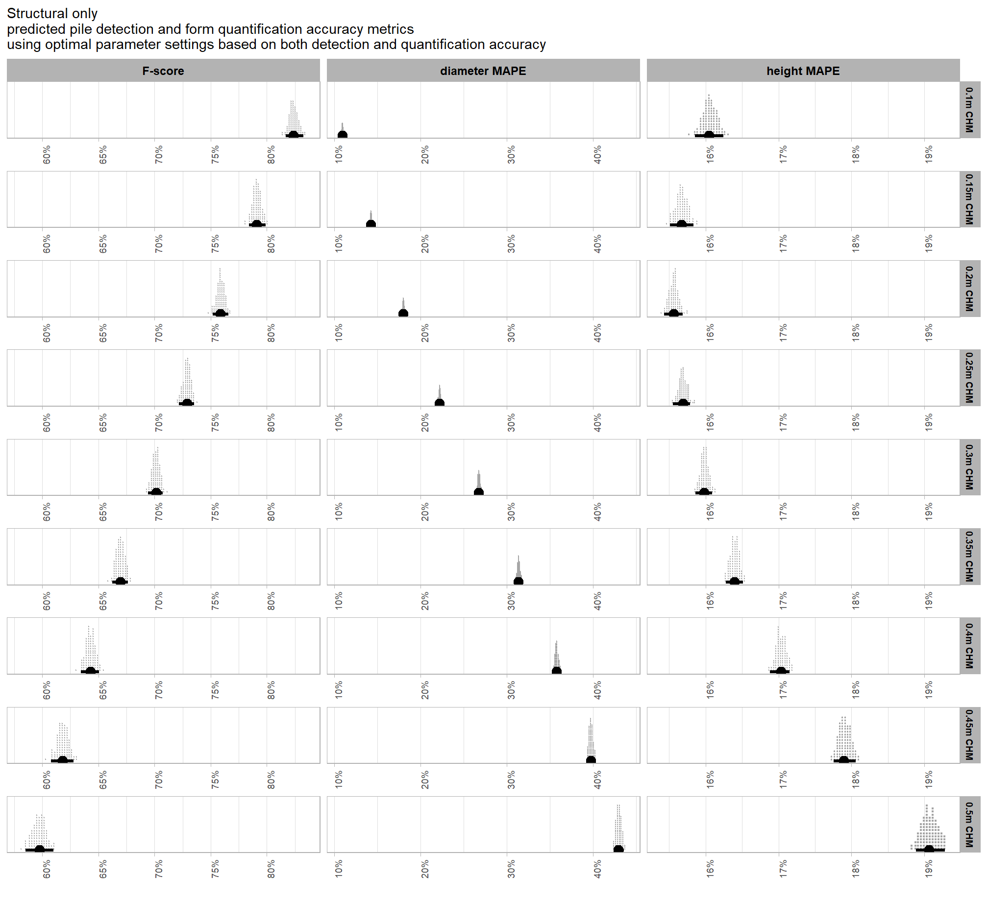
let’s table the HDI of the predicted accuracy metrics
# summarize it
best_balanced_accuracy_combos_long %>%
  dplyr::filter(method_input_data=="structural only") %>%
  dplyr::ungroup() %>%
  # filter for accuracy metrics
  dplyr::filter(name=="f_score" | stringr::str_ends(name, "_mape")) %>%
  dplyr::mutate(
    name = name %>%
      stringr::str_replace_all("_mape", "_MAPE") %>%
      stringr::str_replace_all("f_score", "F-score") %>%
      stringr::str_replace_all("_", " ") %>%
      stringr::str_squish() %>%
      factor(ordered = T) %>%
      forcats::fct_relevel("F-score")
  ) %>%
  dplyr::group_by(chm_res_m_desc, method_input_data, name) %>%
  dplyr::summarise(
    # get median_hdi
    median_hdi_est = tidybayes::median_hdci(value)$y
    , median_hdi_lower = tidybayes::median_hdci(value)$ymin
    , median_hdi_upper = tidybayes::median_hdci(value)$ymax
  ) %>%
  dplyr::ungroup() %>%
  dplyr::mutate(dplyr::across(
    tidyselect::starts_with("median_hdi")
    , ~ scales::percent(.x,accuracy=.1)
  )) %>%
  dplyr::select(-method_input_data) %>%
  # table it
  kableExtra::kbl(
    caption = paste0(
     "Structural only"
     , "<br>predicted pile detection and form quantification accuracy metrics"
     , "<br>using optimal parameter settings based on both detection and quantification accuracy"
    )
    , col.names = c(
      "CHM Resolution", "metric"
      , c("median", "HDI low", "HDI high")
    )
    , escape = F
  ) %>%
  kableExtra::kable_styling() %>%
  kableExtra::collapse_rows(columns = 1, valign = "top") %>%
  kableExtra::add_header_above(c(
    " "=2
    , "predicted value" = 3
  )) %>%
kableExtra::scroll_box(height = "8in")| CHM Resolution | metric | median | HDI low | HDI high |
|---|---|---|---|---|
| 0.1m CHM | F-score | 82.4% | 81.7% | 83.2% |
| diameter MAPE | 11.0% | 10.8% | 11.1% | |
| height MAPE | 16.0% | 15.9% | 16.2% | |
| 0.15m CHM | F-score | 79.1% | 78.4% | 79.9% |
| diameter MAPE | 14.3% | 14.1% | 14.4% | |
| height MAPE | 15.7% | 15.5% | 15.8% | |
| 0.2m CHM | F-score | 75.9% | 75.2% | 76.6% |
| diameter MAPE | 18.0% | 17.9% | 18.2% | |
| height MAPE | 15.6% | 15.4% | 15.7% | |
| 0.25m CHM | F-score | 72.9% | 72.2% | 73.5% |
| diameter MAPE | 22.2% | 22.0% | 22.4% | |
| height MAPE | 15.7% | 15.6% | 15.8% | |
| 0.3m CHM | F-score | 70.2% | 69.4% | 70.7% |
| diameter MAPE | 26.8% | 26.6% | 27.1% | |
| height MAPE | 16.0% | 15.9% | 16.1% | |
| 0.35m CHM | F-score | 67.0% | 66.2% | 67.6% |
| diameter MAPE | 31.4% | 31.1% | 31.7% | |
| height MAPE | 16.4% | 16.3% | 16.5% | |
| 0.4m CHM | F-score | 64.3% | 63.4% | 65.1% |
| diameter MAPE | 35.8% | 35.5% | 36.2% | |
| height MAPE | 17.0% | 16.9% | 17.2% | |
| 0.45m CHM | F-score | 61.8% | 60.8% | 62.8% |
| diameter MAPE | 39.8% | 39.3% | 40.2% | |
| height MAPE | 17.9% | 17.8% | 18.1% | |
| 0.5m CHM | F-score | 59.8% | 58.5% | 61.0% |
| diameter MAPE | 43.0% | 42.5% | 43.6% | |
| height MAPE | 19.1% | 18.9% | 19.3% |
9.5 Balanced Accuracy Validation
let’s test these optimal settings on the actual data to see how close our model came to properly predicting the accuracies. we’ll test using the data fusion method since we have the RGB data
9.5.1 Detection
remember the optimal parameter settings we identified assuming we have spectral data for a data fusion approach? we’ll use those settings for the structural parameters and set the spectral_weight parameter to the lower end of it’s 95% HDI to be less restrictive with the spectral filtering (e.g. if HDI includes ‘4’ and ‘5’, use ‘4’) while maintaining high anticipated accuracy because these HDI’s include the full range of optimal settings based on our balanced accuracy.
# remember the optimal_param_settings!
optimal_temp <-
  optimal_param_settings %>%
  dplyr::filter(method_input_data == "structural+spectral") %>%
  dplyr::mutate(
    median_hdi_est = dplyr::case_when(
      name == "spectral_weight" ~ median_hdi_lower
      , T ~ median_hdi_est
    )
  ) %>%
  dplyr::select(name,median_hdi_est) %>%
  tidyr::pivot_wider(names_from = name, values_from = median_hdi_est) %>%
  # add on the fixed values
  dplyr::bind_cols(
    structural_params_settings %>% dplyr::select(max_ht_m,max_area_m2)
  )
# huh?
optimal_temp %>% dplyr::glimpse()
## Rows: 1
## Columns: 6
## $ chm_res_m <dbl> 0.1
## $ circle_fit_iou_pct <dbl> 0.46
## $ convexity_pct <dbl> 0.08
## $ spectral_weight <dbl> 4
## $ max_ht_m <dbl> 2.3
## $ max_area_m2 <dbl> 46first, we need to read in the CHM data at the optimal resolution as predicted by the model
# set chm res
chm_res_m_temp <- optimal_temp$chm_res_m
dir_temp <- paste0("../data/point_cloud_processing_delivery_chm",chm_res_m_temp,"m")
# do it
if(!dir.exists(dir_temp)){
  # cloud2trees
  cloud2raster_ans <- cloud2trees::cloud2raster(
    output_dir = "../data"
    , input_las_dir = "f:\\PFDP_Data\\p4pro_images\\P4Pro_06_17_2021_half_half_optimal\\2_densification\\point_cloud"
    , accuracy_level = 2
    , keep_intrmdt = T
    , dtm_res_m = 0.25
    , chm_res_m = chm_res_m_temp
    , min_height = 0 # effectively generates a DSM based on non-ground points
  )
  # rename
  file.rename(from = "../data/point_cloud_processing_delivery", to = dir_temp)
}else{
  dtm_temp <- terra::rast( file.path(dir_temp, "dtm_0.25m.tif") )
  chm_temp <- terra::rast( file.path(dir_temp, paste0("chm_", chm_res_m_temp,"m.tif")) )

  cloud2raster_ans <- list(
    "dtm_rast" = dtm_temp
    , "chm_rast" = chm_temp
  )
}
we’ll only work with the CHM in the study unit boundary plus a buffer to limit the amount of data we process
chm_rast_temp <- cloud2raster_ans$chm_rast %>%
  terra::crop(
    stand_boundary %>%
      sf::st_buffer(2) %>%
      terra::vect() %>%
      terra::project(terra::crs(cloud2raster_ans$chm_rast))
  ) %>%
  terra::mask(
    stand_boundary %>%
      sf::st_buffer(2) %>%
      terra::vect() %>%
      terra::project(terra::crs(cloud2raster_ans$chm_rast))
  )
# # huh?
# chm_rast_temp %>%
#   terra::aggregate(fact = 2, na.rm=T) %>%  #, fun = "median", cores = lasR::half_cores(), na.rm = T) %>%
#   terra::plot(col = viridis::plasma(100), axes = F)
#   terra::plot(
#     stand_boundary %>%
#       terra::vect() %>%
#       terra::project(terra::crs(cloud2raster_ans$chm_rast))
#     , add = T, border = "black", col = NA, lwd = 1.2
#   )
#   terra::plot(
#     slash_piles_polys %>%
#       terra::vect() %>%
#       terra::project(terra::crs(cloud2raster_ans$chm_rast))
#     , add = T, border = "blue", col = NA, lwd = 1.2
#   )
we’re going to use our handy-dandy slash_pile_detect_watershed() function we defined in this earlier section.
outdir_temp <- "../data/PFDP_Data/PFDP_SlashPiles/"
fnm_temp <- file.path(outdir_temp,"structural_candidate_segments.gpkg")
if(!file.exists(fnm_temp)){
  set.seed(77)
  slash_pile_detect_watershed_ans <- slash_pile_detect_watershed(
    chm_rast = chm_rast_temp
    #### height and area thresholds for the detected piles
    # these should be based on data from the literature or expectations based on the prescription
    , max_ht_m = optimal_temp$max_ht_m # set the max expected pile height
    , min_ht_m = 0.5 # set the min expected pile height
    , min_area_m2 = 2 # set the min expected pile area # (5*0.3048)^2 = prescription minimum = 2.322 # ((5*0.95)*0.3048)^2 = 2.1 = 5% less than minimum
    , max_area_m2 = optimal_temp$max_area_m2 # set the max expected pile area
    #### irregularity filtering
    # 1 = perfectly convex (no inward angles); 0 = so many inward angles
    # values closer to 1 remove more irregular segments;
      # values closer to 0 keep more irregular segments (and also regular segments)
    # these will all be further filtered for their circularity and later smoothed to remove blocky edges
    # and most inward angles by applying a convex hull to the original detected segment
    , convexity_pct = optimal_temp$convexity_pct # min required overlap between the predicted pile and the convex hull of the predicted pile
    #### circularity filtering
    # 1 = perfectly circular; 0 = not circular (e.g. linear) but also circular
    # min required IoU between the predicted pile and the best fit circle of the predicted pile
    , circle_fit_iou_pct = optimal_temp$circle_fit_iou_pct
    #### shape refinement & overlap removal
    ## smooth_segs = T ... convex hulls of raster detected segments are returned, any that overlap are removed
    ## smooth_segs = F ... raster detected segments are returned (blocky) if they meet all prior rules
    , smooth_segs = T
  )
  # save
  slash_pile_detect_watershed_ans %>% sf::st_write(fnm_temp, append = F)
}else{
  slash_pile_detect_watershed_ans <- sf::st_read(fnm_temp, quiet=T)
}
# what did we get?
slash_pile_detect_watershed_ans %>% dplyr::glimpse()
## Rows: 162
## Columns: 8
## $ pred_id <int> 1, 2, 3, 5, 6, 7, 8, 9, 10, 11, 12, 13, 14, 15, 16, 17…
## $ area_m2 <dbl> 16.610, 40.330, 5.985, 8.365, 45.635, 18.900, 38.120, …
## $ volume_m3 <dbl> 10.676970, 40.098363, 5.079741, 9.044556, 46.122434, 1…
## $ max_height_m <dbl> 2.235, 2.300, 2.219, 2.300, 2.300, 2.300, 2.300, 2.300…
## $ volume_per_area <dbl> 0.6428037, 0.9942565, 0.8487454, 1.0812380, 1.0106811,…
## $ pct_chull <dbl> 0.6688742, 0.6020332, 0.7084378, 0.7136880, 0.7242248,…
## $ diameter_m <dbl> 7.564390, 9.323626, 3.511410, 3.832754, 8.475848, 6.35…
## $ geom <POLYGON [m]> POLYGON ((499475 4317902, 4..., POLYGON ((4994…Now we’ll filter the structurally-detected candidate slash piles using the RGB spectral data with the polygon_spectral_filtering() function we defined in this earlier section. if you were wondering, yes, this function is also handy-dandy.
final_predicted_slash_piles <- polygon_spectral_filtering(
  sf_data = slash_pile_detect_watershed_ans
  , rgb_rast = ortho_rast
  # define the band index
  , red_band_idx = 1
  , green_band_idx = 2
  , blue_band_idx = 3
  # spectral weighting
  , spectral_weight = optimal_temp$spectral_weight
)
# add is_in_stand
final_predicted_slash_piles <- final_predicted_slash_piles %>%
  dplyr::mutate(
    is_in_stand = pred_id %in% (
      final_predicted_slash_piles %>%
      sf::st_intersection(stand_boundary %>% sf::st_transform(sf::st_crs(final_predicted_slash_piles))) %>%
      sf::st_drop_geometry() %>%
      dplyr::pull(pred_id)
    )
  )
what did we get?
## Rows: 138
## Columns: 24
## $ pred_id          <int> 1, 2, 6, 7, 8, 9, 10, 12, 13, 14, 15, 16, 17, 20, 23,…
## $ area_m2          <dbl> 16.610, 40.330, 45.635, 18.900, 38.120, 24.750, 27.76…
## $ volume_m3        <dbl> 10.676970, 40.098363, 46.122434, 16.298983, 44.237940…
## $ max_height_m     <dbl> 2.235, 2.300, 2.300, 2.300, 2.300, 2.300, 2.300, 2.29…
## $ volume_per_area  <dbl> 0.6428037, 0.9942565, 1.0106811, 0.8623801, 1.1604916…
## $ pct_chull        <dbl> 0.6688742, 0.6020332, 0.7242248, 0.6248677, 0.7678384…
## $ diameter_m       <dbl> 7.564390, 9.323626, 8.475848, 6.350591, 7.564390, 6.3…
## $ rast_agg_grvi    <dbl> 0.015843167, 0.019939091, -0.025123385, 0.025851542, …
## $ rast_agg_rgri    <dbl> 0.9688079, 0.9609014, 1.0515417, 0.9495998, 1.0410348…
## $ rast_agg_vdvi    <dbl> 0.057569480, 0.062395341, 0.005857862, -0.021179659, …
## $ rast_agg_rgbvi   <dbl> 0.11875952, 0.12856891, 0.01387664, -0.03608864, -0.0…
## $ rast_agg_exg     <dbl> 0.078261125, 0.084960841, 0.007825763, -0.028041575, …
## $ rast_agg_exr     <dbl> 0.12790022, 0.12446414, 0.15849203, 0.10745823, 0.148…
## $ rast_agg_exgr    <dbl> -0.050100115, -0.040813919, -0.150284527, -0.13186515…
## $ rast_agg_bi      <dbl> 0.37303904, 0.39702669, 0.53180724, 0.11501747, 0.455…
## $ rast_agg_sat     <dbl> 0.18757563, 0.20254081, 0.11597003, 0.15812179, 0.054…
## $ geom             <POLYGON [m]> POLYGON ((499475 4317902, 4..., POLYGON ((499…
## $ inrange_th_exgr  <dbl> 1, 1, 1, 1, 1, 1, 1, 1, 1, 1, 1, 1, 1, 1, 1, 1, 1, 1,…
## $ inrange_th_rgri  <dbl> 1, 1, 1, 1, 1, 1, 1, 1, 1, 1, 1, 1, 1, 1, 1, 1, 1, 1,…
## $ inrange_th_vdvi  <dbl> 0, 0, 1, 1, 1, 1, 1, 1, 1, 1, 1, 1, 1, 1, 1, 1, 1, 1,…
## $ inrange_th_bi    <dbl> 1, 1, 1, 1, 1, 1, 1, 1, 1, 1, 1, 1, 1, 0, 0, 1, 1, 1,…
## $ inrange_th_sat   <dbl> 1, 1, 1, 1, 1, 1, 1, 1, 1, 1, 1, 1, 1, 1, 1, 1, 1, 1,…
## $ inrange_th_votes <dbl> 4, 4, 5, 5, 5, 5, 5, 5, 5, 5, 5, 5, 5, 4, 4, 5, 5, 5,…
## $ is_in_stand <lgl> TRUE, TRUE, TRUE, TRUE, TRUE, TRUE, TRUE, TRUE, TRUE,…how many piles were removed?
# how many piles were removed?
nrow(slash_pile_detect_watershed_ans)-nrow(final_predicted_slash_piles)
## [1] 24# what proportion were removed?
scales::percent(
(nrow(slash_pile_detect_watershed_ans)-nrow(final_predicted_slash_piles))/nrow(slash_pile_detect_watershed_ans)
, accuracy=0.1
)## [1] "14.8%"9.5.2 Instance Match & Accuracy Assessment
now apply the instance matching process we outlined in this earlier section to establish True Positives (TP), False Positives (FP, commissions), and False Negatives (FN, omissions)
# ground truth and prediction matching process
ground_truth_prediction_match_ans <- ground_truth_prediction_match(
  ground_truth =
    slash_piles_polys %>%
    dplyr::filter(is_in_stand) %>%
    dplyr::arrange(desc(field_diameter_m)) %>%
    sf::st_transform(sf::st_crs(final_predicted_slash_piles))
  , gt_id = "pile_id"
  , predictions = final_predicted_slash_piles %>% dplyr::filter(is_in_stand)
  , pred_id = "pred_id"
  , min_iou_pct = 0.05
)
# add data from gt and pred piles
ground_truth_prediction_match_ans <-
  ground_truth_prediction_match_ans %>%
  # add area of gt
  dplyr::left_join(
    slash_piles_polys %>%
      sf::st_drop_geometry() %>%
      dplyr::filter(is_in_stand) %>%
      dplyr::select(
        pile_id
        , image_gt_area_m2
        , image_gt_diameter_m
        , field_gt_volume_m3
        , height_m
        , field_diameter_m
      ) %>%
      dplyr::rename(
        gt_height_m = height_m
        , gt_diameter_m = field_diameter_m
        , gt_area_m2 = image_gt_area_m2
        , gt_volume_m3 = field_gt_volume_m3
      ) %>%
      dplyr::mutate(pile_id=as.numeric(pile_id))
    , by = "pile_id"
  ) %>%
  # add info from predictions
  dplyr::left_join(
    slash_pile_detect_watershed_ans %>%
      sf::st_drop_geometry() %>%
      dplyr::select(
        pred_id
        , area_m2, volume_m3, max_height_m, diameter_m
      ) %>%
      dplyr::rename(
        pred_area_m2 = area_m2, pred_volume_m3 = volume_m3
        , pred_height_m = max_height_m, pred_diameter_m = diameter_m
      )
    , by = dplyr::join_by(pred_id)
  ) %>%
  dplyr::mutate(
    ### calculate these based on the formulas below...agg_ground_truth_match() depends on those formulas
    # ht diffs
    diff_height_m = pred_height_m-gt_height_m
    , pct_diff_height_m = (gt_height_m-pred_height_m)/gt_height_m
    # diameter
    , diff_field_diameter_m = pred_diameter_m-gt_diameter_m
    , pct_diff_field_diameter_m = (gt_diameter_m-pred_diameter_m)/gt_diameter_m
    # image diameter
    , diff_image_diameter_m = pred_diameter_m-image_gt_diameter_m
    , pct_diff_image_diameter_m = (image_gt_diameter_m-pred_diameter_m)/image_gt_diameter_m
    # area diffs
    , diff_area_m2 = pred_area_m2-gt_area_m2
    , pct_diff_area_m2 = (gt_area_m2-pred_area_m2)/gt_area_m2

  )
# huh?
ground_truth_prediction_match_ans %>% dplyr::glimpse()
## Rows: 151
## Columns: 23
## $ pile_id <dbl> 194, 82, 76, 8, 187, 77, 189, 132, 111, 131,…
## $ i_area <dbl> 44.907459, 36.745987, 19.083370, 27.643199, …
## $ u_area <dbl> 54.767766, 41.666730, 22.405358, 30.096676, …
## $ iou <dbl> 0.8199615, 0.8819024, 0.8517324, 0.9184802, …
## $ pred_id <int> 6, 8, 115, 13, 12, 10, 26, 104, 47, 141, 150…
## $ match_grp <ord> true positive, true positive, true positive,…
## $ gt_area_m2 <dbl> 54.040225, 40.292717, 21.308728, 28.909875, …
## $ image_gt_diameter_m <dbl> 8.966741, 7.892174, 5.909959, 7.595808, 6.88…
## $ gt_volume_m3 <dbl> 183.079674, 97.299997, 91.178437, 75.349118,…
## $ gt_height_m <dbl> 6.4008, 4.2672, 4.7244, 4.2672, 3.2004, 2.43…
## $ gt_diameter_m <dbl> 8.53440, 7.62000, 7.01040, 6.70560, 6.46176,…
## $ pred_area_m2 <dbl> 45.635, 38.120, 20.180, 28.830, 24.930, 27.7…
## $ pred_volume_m3 <dbl> 46.122434, 44.237940, 16.008302, 30.692573, …
## $ pred_height_m <dbl> 2.300, 2.300, 1.731, 2.298, 2.299, 2.300, 2.…
## $ pred_diameter_m <dbl> 8.475848, 7.564390, 5.679789, 7.375636, 6.64…
## $ diff_height_m <dbl> -4.10080005, -1.96720005, -2.99340005, -1.96…
## $ pct_diff_height_m <dbl> 0.6406699237, 0.4610048856, 0.6336042785, 0.…
## $ diff_field_diameter_m <dbl> -0.05855196, -0.05560974, -1.33061127, 0.670…
## $ pct_diff_field_diameter_m <dbl> 0.006860700, 0.007297866, 0.189805328, -0.09…
## $ diff_image_diameter_m <dbl> -0.49089339, -0.32778417, -0.23016998, -0.22…
## $ pct_diff_image_diameter_m <dbl> 0.05474602, 0.04153281, 0.03894612, 0.028986…
## $ diff_area_m2 <dbl> -8.4052248, -2.1727174, -1.1287281, -0.07987…
## $ pct_diff_area_m2 <dbl> 0.155536452, 0.053923327, 0.052970225, 0.002…Now we’ll aggregate the instance matching results to calculate overall performance assessment metrics. Here, we take the counts of True Positives (TP), False Positives (FP, commissions), and False Negatives (FN, omissions), to determine overall accuracy. This aggregation will give us two types of results:
- detection accuracy metrics: such as Recall, Precision, and F-score, are calculated directly by aggregating these raw TP, FP, and FN counts and quantifies the method’s ability to find the piles
- quantification accuracy metrics: such as RMSE, MAPE, and Mean Error of pile form measurements (e.g. height, diameter) are calculated by aggregating the differences between the estimated pile attributes and the ground truth values for instances classified as True Positives. These metrics tell us about the method’s ability to accurately quantify the form of the piles it successfully identified
agg_ground_truth_match_ans <- agg_ground_truth_match(ground_truth_prediction_match_ans = ground_truth_prediction_match_ans)
# huh?
# agg_ground_truth_match_ans %>% dplyr::glimpse()
let’s table the relevant accuracy metrics
kbl_agg_gt_match <- function(
  agg_ground_truth_match_df
  , caption = "pile detection and form quantification accuracy metrics"
) {
  # let's table the most relevant metrics
  agg_ground_truth_match_df %>%
  # first select to arrange eval_metric
  dplyr::select(
    # detection cnt
    tp_n, fn_n, fp_n
    # detection
    , f_score, recall, precision
    # quantification
    , tidyselect::ends_with("_mean")
    , tidyselect::ends_with("_rmse")
    # , tidyselect::ends_with("_rrmse")
    , tidyselect::ends_with("_mape")
  ) %>%
  # second select to arrange pile_metric
  dplyr::select(
    # detection cnt
    tp_n, fn_n, fp_n
    # detection
    , f_score, recall, precision
    # quantification
    , c(tidyselect::contains("volume") & !tidyselect::contains("paraboloid"))
    , tidyselect::contains("area")
    , tidyselect::contains("height")
    , tidyselect::contains("diameter")
  ) %>%
  dplyr::mutate(
    dplyr::across(
      .cols = c(f_score, recall, precision, tidyselect::ends_with("_mape"))
      , .fn = ~ scales::percent(.x, accuracy = 1)
    )
    , dplyr::across(
      .cols = c(tidyselect::ends_with("_mean"))
      , .fn = ~ scales::comma(.x, accuracy = 0.01)
    )
    , dplyr::across(
      .cols = c(tidyselect::ends_with("_rmse"))
      , .fn = ~ scales::comma(.x, accuracy = 0.1)
    )
    , dplyr::across(
      .cols = c(tidyselect::ends_with("_n"))
      , .fn = ~ scales::comma(.x, accuracy = 1)
    )
  ) %>%
  tidyr::pivot_longer(
    cols = c(
      tidyselect::ends_with("_n")
      , f_score, recall, precision
      , tidyselect::ends_with("_rmse")
      , tidyselect::ends_with("_rrmse")
      , tidyselect::ends_with("_mean")
      , tidyselect::ends_with("_mape")
    )
    , names_to = "metric"
    , values_to = "value"
  ) %>%
  dplyr::mutate(
    eval_metric = metric %>%
      stringr::str_extract("(_rmse|_rrmse|_mean|_mape|f_score|recall|precision|tp_n|fn_n|fp_n)$") %>%
      stringr::str_remove_all("_n$") %>%
      stringr::str_remove_all("_") %>%
      stringr::str_replace_all("mean","me") %>%
      toupper() %>%
      factor(
        ordered = T
        , levels = c("TP","FN","FP", "FSCORE","RECALL","PRECISION", "ME","RMSE","RRMSE","MAPE")
        , labels = c("TP","FN","FP", "F-score","Recall","Precision", "ME","RMSE","RRMSE","MAPE")
      )
    , pile_metric = metric %>%
      stringr::str_remove("(_rmse|_rrmse|_mean|_mape)$") %>%
      stringr::str_extract("(paraboloid_volume|volume|area|height|diameter)") %>%
      dplyr::coalesce("detection") %>%
      stringr::str_c(
        dplyr::case_when(
          stringr::str_detect(metric,"(field|image)") ~ paste0(" (", stringr::str_extract(metric,"(field|image)"), ")")
          , T ~ ""
        )
      ) %>%
      stringr::str_replace("area", "area m<sup>2</sup>") %>%
      stringr::str_replace("volume", "volume m<sup>3</sup>") %>%
      stringr::str_replace("diameter", "diameter m") %>%
      stringr::str_replace("height", "height m") %>%
      stringr::str_to_sentence()
  ) %>%
  dplyr::mutate(
    pile_metric = dplyr::case_when(
      pile_metric == "Detection" & eval_metric %in% c("TP","FN","FP") ~ "Detection Count"
      , T ~ pile_metric
    )
    , sorter = dplyr::case_when(
      pile_metric=="Detection Count" ~ 1
      , pile_metric=="Detection" ~ 2
      , T ~ 3
    )
  ) %>%
  dplyr::arrange(sorter, pile_metric, eval_metric) %>%
  dplyr::select(pile_metric,eval_metric,value) %>%
  kableExtra::kbl(
    caption = caption
    , col.names = c(
      ".", ""
      , "value"
    )
    , escape = F
  ) %>%
  kableExtra::kable_styling(font_size = 12) %>%
  kableExtra::collapse_rows(columns = 1, valign = "top")
}
use the function we just defined to make a nice summary table
# do it
kbl_agg_gt_match(
  agg_ground_truth_match_ans
  , caption = "pile detection and form quantification accuracy metrics<br>data fusion ponderosa pine training site"
)| . | value | |
|---|---|---|
| Detection Count | TP | 107 |
| FN | 14 | |
| FP | 30 | |
| Detection | F-score | 83% |
| Recall | 88% | |
| Precision | 78% | |
| Area m2 | ME | -0.63 |
| RMSE | 2.1 | |
| MAPE | 12% | |
| Diameter m (field) | ME | 0.21 |
| RMSE | 0.6 | |
| MAPE | 11% | |
| Diameter m (image) | ME | -0.17 |
| RMSE | 0.4 | |
| MAPE | 8% | |
| Height m | ME | -0.20 |
| RMSE | 0.7 | |
| MAPE | 15% |
# save the table for full comparison at the very end
all_agg_ground_truth_match_ans_fp <- file.path("../data/","all_agg_ground_truth_match_ans.csv")
agg_ground_truth_match_ans %>%
  # join on aggregated form quantifications that we have for all
  dplyr::bind_cols(
    ground_truth_prediction_match_ans %>%
      dplyr::ungroup() %>%
      dplyr::summarise(
        dplyr::across(
          c(image_gt_diameter_m, pred_diameter_m, gt_area_m2, pred_area_m2, pred_volume_m3, pred_height_m)
          , ~ sum(.x, na.rm = TRUE)
        )
      )
  ) %>%
  dplyr::mutate(site = "ponderosa pine training site") %>%
  # dplyr::glimpse()
  readr::write_csv(file = all_agg_ground_truth_match_ans_fp, append = F, progress = F)
let’s compare these with the predicted accuracies from the model
best_balanced_accuracy_combos %>%
  # get rid of vars we fixed
  dplyr::select(-c(max_ht_m, max_area_m2)) %>%
  dplyr::mutate(
    spectral_weight = spectral_weight %>% as.character() %>% as.numeric()
  ) %>%
  tidyr::pivot_longer(cols = -c(.draw,method_input_data)) %>%
  dplyr::ungroup() %>%
  # filter for accuracy metrics
  dplyr::filter(name=="f_score" | stringr::str_ends(name, "_mape")) %>%
  dplyr::mutate(
    name = name %>%
      stringr::str_replace_all("_mape", "_MAPE") %>%
      stringr::str_replace_all("f_score", "F-score") %>%
      stringr::str_replace_all("_", " ") %>%
      stringr::str_squish() %>%
      factor(ordered = T) %>%
      forcats::fct_relevel("F-score")
  ) %>%
  dplyr::filter(method_input_data == "structural+spectral") %>%
  ggplot2::ggplot(mapping = ggplot2::aes(x = value)) +
  tidybayes::stat_dotsinterval(
    point_interval = "median_hdci", .width = c(0.99)
    , quantiles = 100
    , point_size = 3
  ) +
  ggplot2::geom_vline(
    data =
      agg_ground_truth_match_ans %>%
      dplyr::select(f_score,pct_diff_field_diameter_m_mape,pct_diff_height_m_mape) %>%
      dplyr::rename(
        diameter_mape=pct_diff_field_diameter_m_mape
        , height_mape=pct_diff_height_m_mape
      ) %>%
      tidyr::pivot_longer(cols = dplyr::everything()) %>%
      dplyr::ungroup() %>%
      # filter for accuracy metrics
      dplyr::filter(name=="f_score" | stringr::str_ends(name, "_mape")) %>%
      dplyr::mutate(
        name = name %>%
          stringr::str_replace_all("_mape", "_MAPE") %>%
          stringr::str_replace_all("f_score", "F-score") %>%
          stringr::str_replace_all("_", " ") %>%
          stringr::str_squish() %>%
          factor(ordered = T) %>%
          forcats::fct_relevel("F-score")
      )
    , mapping = ggplot2::aes(xintercept=value)
    , color = "navy", lwd = 2, alpha = 0.7
  ) +
  ggplot2::facet_grid(
    cols = dplyr::vars(name)
    , scales = "free_x"
    , axes = "all_x"
  ) +
  ggplot2::scale_y_continuous(NULL, breaks = NULL) +
  ggplot2::scale_x_continuous(labels = scales::percent, expand = ggplot2::expansion(mult = c(1.1,1.1))) +
  ggplot2::labs(
    x=""
    , subtitle = paste0(
      "Data Fusion predictions with actual results in blue"
     , "\npredicted pile detection and form quantification accuracy metrics"
     , "\nusing optimal parameter settings based on both detection and quantification accuracy"
    )
  ) +
  ggplot2::theme_light() +
  ggplot2::theme(
    legend.position = "none"
    , strip.text = ggplot2::element_text(size = 10, color = "black", face = "bold")
    , axis.text.x = ggplot2::element_text(size = 8, angle = 90)
  )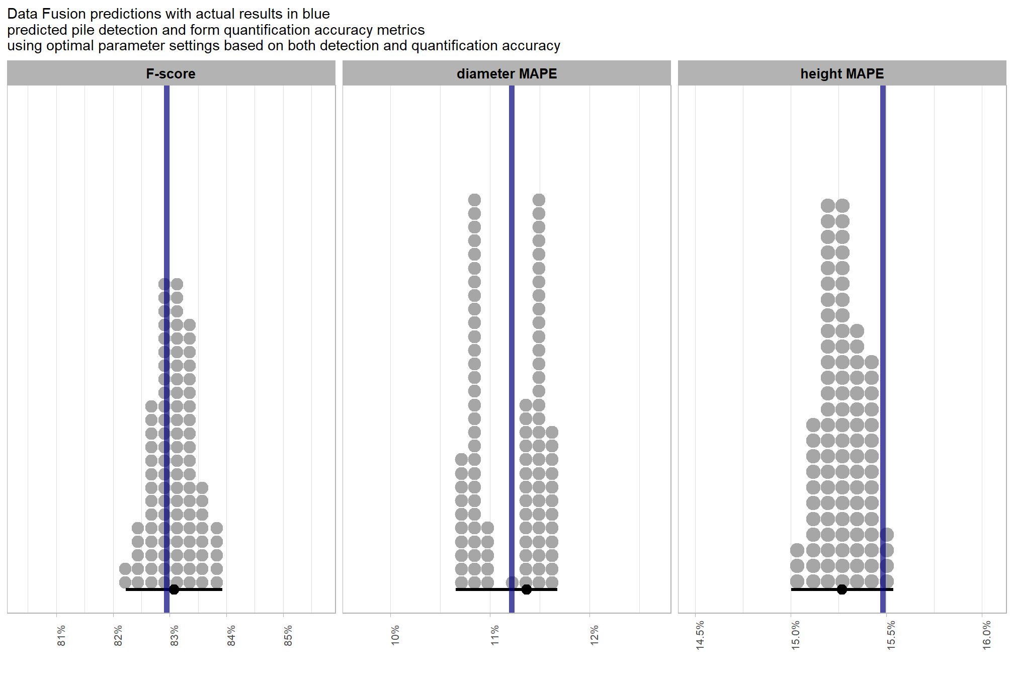
pretty close!
let’s now look at the summary stats of ground truth piles
kbl_form_sum_stats(
  slash_piles_polys %>% dplyr::filter(is_in_stand) %>% dplyr::select(!tidyselect::contains("volume_m3"))
  , caption = "Ground Truth Piles: summary statistics for form measurements<br>ponderosa pine training site"
)| # piles | Metric | Mean | Std Dev | q 10% | Median | q 90% | Range |
|---|---|---|---|---|---|---|---|
| 121 | Height m | 2.2 | 0.8 | 1.7 | 2.0 | 2.3 | 1.5—6.4 |
| Diameter m (image) | 3.8 | 1.3 | 3.0 | 3.5 | 4.5 | 2.6—10.2 | |
| Diameter m (field) | 3.4 | 1.2 | 2.8 | 3.1 | 4.0 | 2.4—9.0 | |
| Area m2 (image) | 9.8 | 9.4 | 5.6 | 7.1 | 11.9 | 3.9—59.3 | |
| Area m2 (field) | 10.5 | 10.2 | 6.2 | 7.6 | 12.3 | 4.7—63.1 |
and let’s look at the summary stats of the predicted piles
kbl_form_sum_stats(
  final_predicted_slash_piles %>% dplyr::filter(is_in_stand)
  , caption = "Predicted Piles: summary statistics for form measurements<br>ponderosa pine training site"
)| # piles | Metric | Mean | Std Dev | q 10% | Median | q 90% | Range |
|---|---|---|---|---|---|---|---|
| 137 | Height m | 1.9 | 0.4 | 1.5 | 2.0 | 2.3 | 0.7—2.3 |
| Diameter m | 3.6 | 1.2 | 2.6 | 3.3 | 4.7 | 2.0—9.3 | |
| Area m2 | 8.2 | 6.8 | 3.6 | 6.4 | 13.1 | 2.4—45.6 | |
| Volume m3 | 7.0 | 7.6 | 2.6 | 5.0 | 10.8 | 0.8—46.1 |
let’s look at these on the RGB
# plot it
ortho_plt_fn(my_ortho_rast = ortho_rast, stand = stand_boundary %>% sf::st_transform(sf::st_crs(ortho_rast)), buffer = 10) +
# ggplot2::ggplot() +
  ggplot2::geom_sf(data = stand_boundary %>% sf::st_transform(sf::st_crs(ortho_rast)), fill = NA, color = "black", lwd = 0.8) +
  ggplot2::geom_sf(
    data =
      slash_piles_polys %>%
      dplyr::filter(is_in_stand) %>%
      dplyr::left_join(
        ground_truth_prediction_match_ans %>%
          dplyr::select(pile_id,match_grp)
        , by = "pile_id"
      ) %>%
      sf::st_transform(sf::st_crs(ortho_rast))
    , mapping = ggplot2::aes(fill = match_grp)
    , color = NA ,alpha=0.6
  ) +
  ggplot2::geom_sf(
    data =
      final_predicted_slash_piles %>%
      dplyr::filter(is_in_stand) %>%
      dplyr::left_join(
        ground_truth_prediction_match_ans %>%
          dplyr::select(pred_id,match_grp)
        , by = "pred_id"
      ) %>%
      sf::st_transform(sf::st_crs(ortho_rast))
    , mapping = ggplot2::aes(fill = match_grp, color = match_grp)
    , alpha = 0
    , lwd = 0.3
  ) +
  ggplot2::scale_fill_manual(values = pal_match_grp, name = "") +
  ggplot2::scale_color_manual(values = pal_match_grp, name = "") +
  ggplot2::theme(legend.position = "top") +
  ggplot2::guides(
    fill = ggplot2::guide_legend(override.aes = list(color = c(NA,NA,pal_match_grp["commission"])))
    , color = "none"
  )
## |---------|---------|---------|---------|========================================= 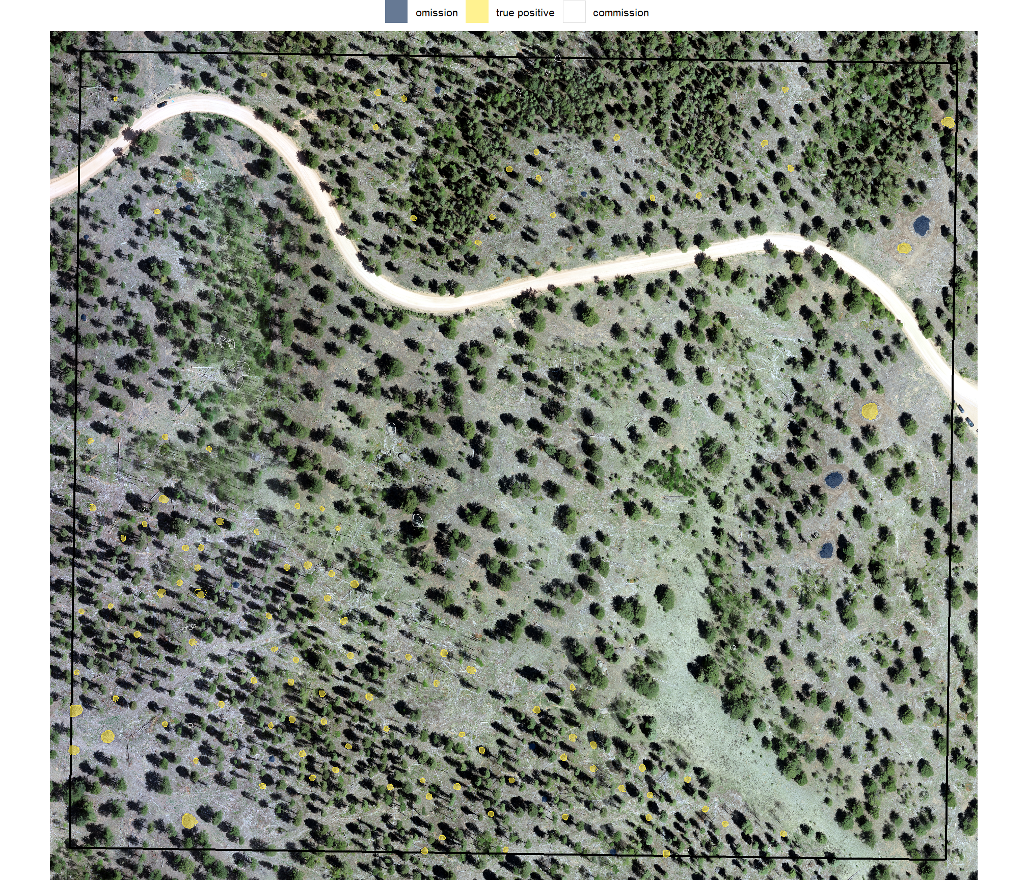
there are many TP matches there!
## # A tibble: 1 × 3
##    tp_n  fp_n  fn_n
##   <dbl> <dbl> <dbl>
## 1   107    30    14
let’s look at some examples on our RGB image
commissions (false positives)
predicted pile outlined in brown
plts_temp <-
  which(ground_truth_prediction_match_ans$match_grp %in% c("commission")) %>%
  sample( min(16,agg_ground_truth_match_ans$fp_n) ) %>%
  purrr::map(function(x){
    dta <- ground_truth_prediction_match_ans %>% dplyr::slice(x)
    pr <- final_predicted_slash_piles %>% dplyr::filter(pred_id==dta$pred_id)
    #plt
    ortho_plt_fn(my_ortho_rast=ortho_rast, stand=sf::st_union(pr), buffer=6) +
      ggplot2::geom_sf(data = pr, fill = NA, color = "brown", lwd = 0.5)
  })
# combine
patchwork::wrap_plots(
  plts_temp
  , ncol = 4
)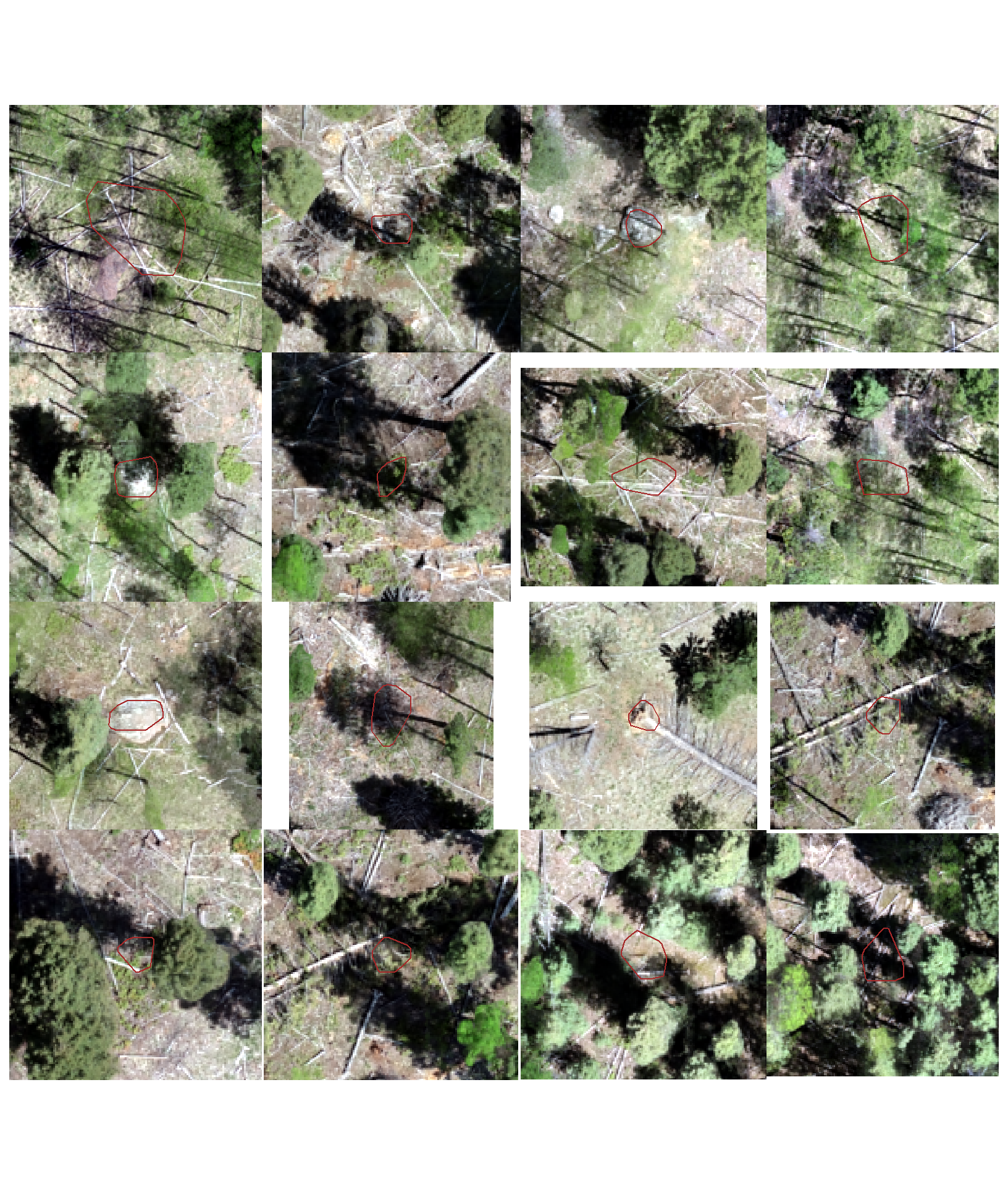
there are rocks, shadows, root bundles, downed trees with branches…
omissions (false negatives)
actual piles outlined in blue
plts_temp <-
  which(ground_truth_prediction_match_ans$match_grp %in% c("omission")) %>%
  sample( min(16,agg_ground_truth_match_ans$fn_n) ) %>%
  purrr::map(function(x){
    dta <- ground_truth_prediction_match_ans %>% dplyr::slice(x)
    gt <- slash_piles_polys %>% dplyr::filter(pile_id==dta$pile_id)

    #plt
    ortho_plt_fn(my_ortho_rast=ortho_rast, stand=sf::st_union(gt), buffer=6) +
      ggplot2::geom_sf(data = gt, fill = NA, color = "blue", lwd = 0.6)
  })
# combine
patchwork::wrap_plots(
  plts_temp
  , ncol = 4
)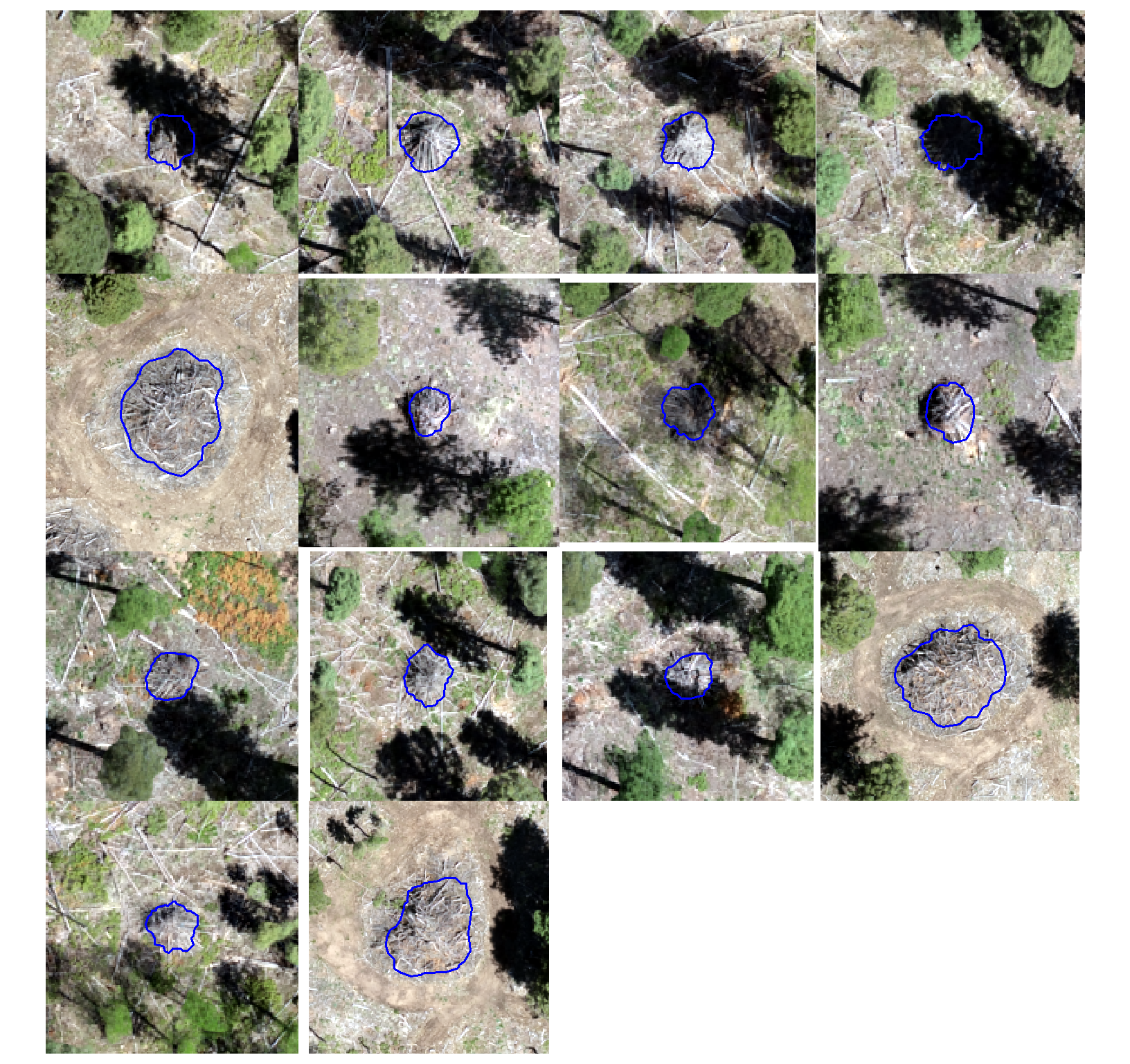
for the most part, those are irregularly shaped or have unexpected spectral signatures (e.g. very white or entirely in dark shadows). however, the machine piles might have been larger than our expected area threshold max_area_m2 or taller than our expected height threshold max_ht_m
9.5.3 Volume Comparison
We restricted our quantification accuracy evaluation to measurements that were directly collected across both sites (i.e. training and validation site). The ground truth dataset only includes direct data for field-measured height, field-measured diameter, and image-annotated area (based on pile perimeters). Accuracy and error metrics, such as ME, RMSE, and MAPE, will be only calculated for these direct measurements.
We excluded quantification accuracy metrics for derived volume because the resulting value would not constitute a true “error”. Comparing our predicted volume to a volume that was not directly measured, but instead calculated using a geometric assumption (like assuming a perfectly circular base and paraboloid shape) would be inappropriate. This is because any resulting difference between the prediction and the ground truth would be a blend of three inseparable factors: the error of the remote-sensing prediction method, the error in the direct field measurements (diameter/height), and the error introduced by the geometric shape assumption. Reporting such combined errors would be misleading, as it would be impossible to isolate the true performance of our remote-sensing method alone.
Instead, data involving derived values of volume based on field measurements and a shape assumption and its comparison to our irregularly shaped CHM-derived volume will be treated simply as data points for insight into the differences. Using geometric shape assumptions for estimating pile volume is the standard practice when implementing prescriptions or preparing for slash pile burning (Hardy 1996; Long & Boston 2014). This comparison will help us understand the discrepancy between our irregularly shaped CHM-derived volume and the volume calculated assuming a perfectly circular base and paraboloid shape with field-measured height and diameter. This approach will still provide valuable context about the impact of the perfectly circular base and paraboloid geometric assumptions without falsely attributing the error of the simplified model to the remote-sensing method itself.
let’s do that now
- ground truth piles
- volume assumes a paraboloid shape, with volume calculated using the field-measured diameter (as the width) and height. we’ll refer to this as “Allometric Field Volume” to indicate the field measurement is derived using a shape assumption.
- predicted piles
- volume calculated from the elevation profile of the irregular predicted pile footprint, without assuming a specific geometric shape. we’ll refer to this as “Predicted Volume” to indicate the predicted measurement is from our CHM-based detection methodology
We would generally expect that the allometric field volume is larger than the predicted volume because the allometric calculation assumes a perfectly regular geometric shape (circular base and paraboloid) based on maximum field dimensions (height and diameter). this process effectively encloses the actual, irregular pile form within a simplified geometric dome which inherently neglects and sits above the actual irregularities and voids in the pile structure, likely leading to an overestimation of the volume.
we already added volume measurements to the TP matches for both the ground truth and predicted piles, summary of that data
ground_truth_prediction_match_ans %>%
  dplyr::filter(match_grp=="true positive") %>%
  dplyr::select(gt_volume_m3, pred_volume_m3) %>%
  summary()
## gt_volume_m3 pred_volume_m3
## Min. : 4.270 Min. : 1.109
## 1st Qu.: 6.564 1st Qu.: 4.276
## Median : 7.497 Median : 5.216
## Mean : 12.375 Mean : 7.136
## 3rd Qu.: 8.746 3rd Qu.: 7.054
## Max. :183.080 Max. :46.122those don’t really look like they match up well…let’s explore
ground_truth_prediction_match_ans %>%
  dplyr::filter(match_grp=="true positive") %>%
  dplyr::mutate(diff_volume_m3 = gt_volume_m3 - pred_volume_m3) %>%
  ggplot2::ggplot(mapping = ggplot2::aes(y = gt_volume_m3, x = pred_volume_m3)) +
  ggplot2::geom_abline(lwd = 1.5) +
  # ggplot2::geom_point(ggplot2::aes(color = diff_volume_m3)) +
  ggplot2::geom_point(color = "navy") +
  ggplot2::geom_smooth(method = "lm", se=F, color = "tomato", linetype = "dashed") +
  ggplot2::scale_color_viridis_c(option = "mako", direction = -1, alpha = 0.8) +
  ggplot2::scale_x_continuous(limits = c(0, max( max(ground_truth_prediction_match_ans$pred_volume_m3,na.rm=T), max(ground_truth_prediction_match_ans$gt_volume_m3,na.rm=T) ) )) +
  ggplot2::scale_y_continuous(limits = c(0, max( max(ground_truth_prediction_match_ans$pred_volume_m3,na.rm=T), max(ground_truth_prediction_match_ans$gt_volume_m3,na.rm=T) ) )) +
  ggplot2::labs(
    y = latex2exp::TeX("allometric field volume $m^3$")
    , x = latex2exp::TeX("predicted volume $m^3$")
    # , color = "image-field\ndiameter diff."
    , subtitle = latex2exp::TeX("bulk volume ($m^3$) comparison")
  ) +
  ggplot2::theme_light()
this is exactly what we expected: for true positive matches, there is a clear systematic difference with the plot showing that the volume calculated using the idealized, regular shape assumption (allometric field volume) is consistently larger than the predicted volume derived from the CHM
let’s check these using lm()
lm_temp <- lm(gt_volume_m3 ~ pred_volume_m3, data = ground_truth_prediction_match_ans %>% dplyr::filter(match_grp=="true positive"))
summary(lm_temp)
##
## Call:
## lm(formula = gt_volume_m3 ~ pred_volume_m3, data = ground_truth_prediction_match_ans %>%
## dplyr::filter(match_grp == "true positive"))
##
## Residuals:
## Min 1Q Median 3Q Max
## -37.174 -3.524 0.247 3.327 66.142
##
## Coefficients:
## Estimate Std. Error t value Pr(>|t|)
## (Intercept) -6.7649 1.5273 -4.429 2.33e-05 ***
## pred_volume_m3 2.6820 0.1517 17.682 < 2e-16 ***
## ---
## Signif. codes: 0 '***' 0.001 '**' 0.01 '*' 0.05 '.' 0.1 ' ' 1
##
## Residual standard error: 11.15 on 105 degrees of freedom
## Multiple R-squared: 0.7486, Adjusted R-squared: 0.7462
## F-statistic: 312.6 on 1 and 105 DF, p-value: < 2.2e-16These linear model results (intercept = -6.76, slope = 2.68) indicate a strong proportional bias that significantly increases with pile size. The high slope (2.68) coupled with the negative intercept (-6.76) indicate that the volume difference is not a simple constant offset (e.g. slope of ~1.0 and intercept of >0 if our hypothesis of consistently higher allometric field volume is true), but rather a scaling issue that is driven by the largest piles. The much larger allometric field volume estimates relative to the CHM-predicted volumes for the largest piles exert a strong influence on the predicted form of the liner model, pulling the slope steeply upward and forcing the intercept below zero as a mathematical artifact. Despite the predicted negative intercept, visual inspection of the data shows that most allometric field volumes are larger than the CHM-predicted volumes, even for smaller piles. The slope value indicates that for every 1 m3 increase in predicted volume, the allometric field volume increases by nearly 2.68 m3. This data suggests that the geometric assumptions of the allometric model potentially introduce substantial scaling error which may limit its reliability (especially for larger piles) for accurately estimating the volume of real-world piles which have heterogeneous footprints and elevation profiles.
before we compare the volume measurements in aggregate, let’s look at their distributions
vol_df_temp <-
  ground_truth_prediction_match_ans %>%
  dplyr::filter(match_grp=="true positive") %>%
  dplyr::select(pile_id,gt_volume_m3,pred_volume_m3) %>%
  tidyr::pivot_longer(cols = -c(pile_id)) %>%
  dplyr::mutate(
    name = factor(
      name
      , ordered = T
      , levels = c("gt_volume_m3","pred_volume_m3")
      , labels = c(
        "allometric field volume"
        , "predicted volume"
      )
    )
  )
# plot dist
vol_df_temp %>%
  ggplot2::ggplot(mapping = ggplot2::aes(x = value, color = name, fill = name)) +
  ggplot2::geom_density(mapping = ggplot2::aes(y=ggplot2::after_stat(scaled)), alpha = 0.7) +
  harrypotter::scale_color_hp_d(option = "lunalovegood") +
  harrypotter::scale_fill_hp_d(option = "lunalovegood") +
  ggplot2::scale_y_continuous(NULL,breaks=NULL) +
  ggplot2::labs(
    color="",fill="",x=latex2exp::TeX("volume $m^3$")
    , subtitle = latex2exp::TeX("bulk volume ($m^3$) comparison of distributions")
  ) +
  ggplot2::theme_light() +
  ggplot2::theme(
    legend.position = "top"
  )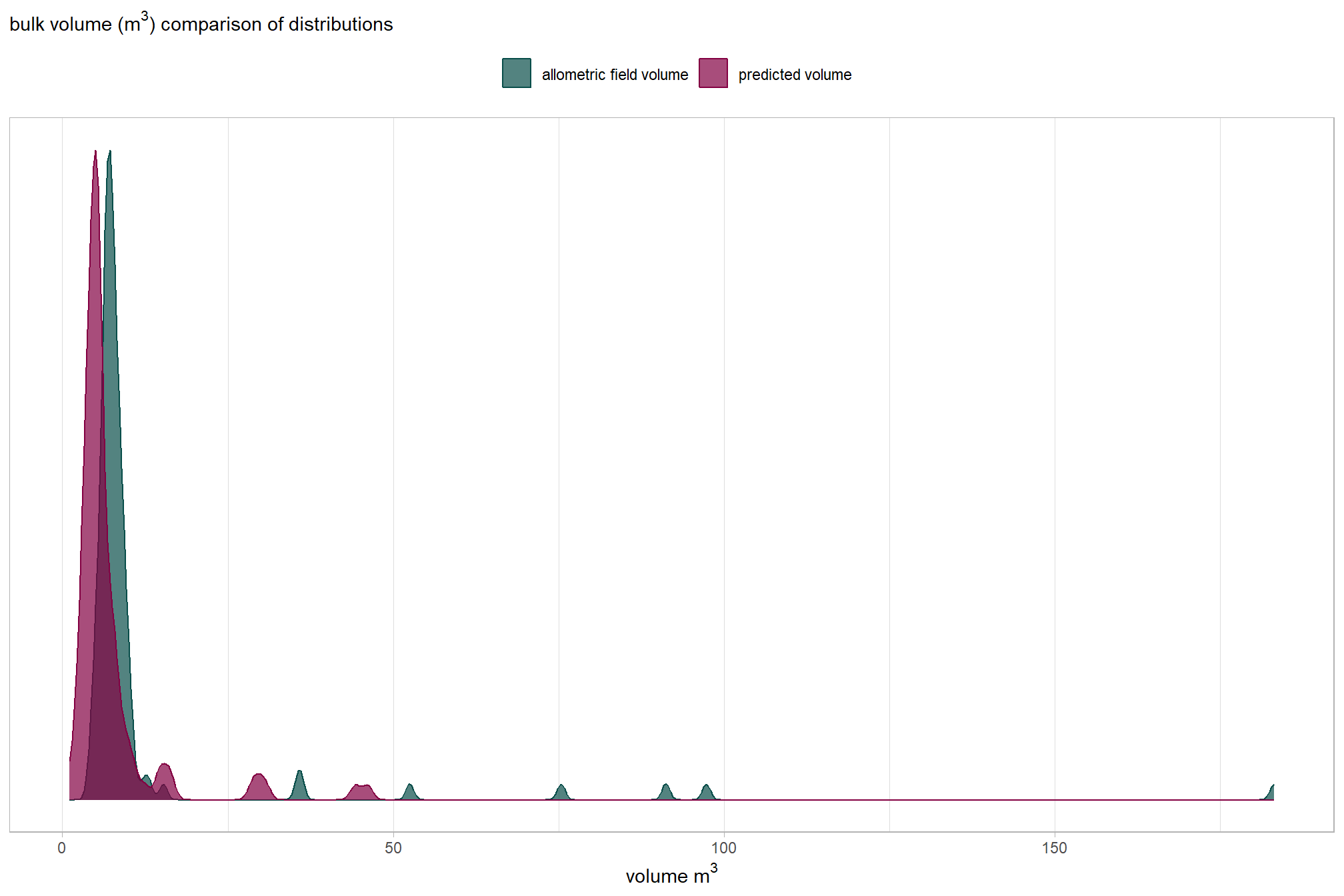
slope plots are neat too
vol_df_temp %>%
  ggplot2::ggplot(
    mapping = ggplot2::aes(x = name, y = value, group = pile_id)
  ) +
  ggplot2::geom_line(key_glyph = "point", alpha = 0.7, color = "gray", lwd = 1.1) +
  ggplot2::geom_point(mapping = ggplot2::aes(color = name), alpha = 0.7, size = 2.5) +
  harrypotter::scale_color_hp_d(option = "lunalovegood") +
  ggplot2::labs(
    color=""
    , y = latex2exp::TeX("volume $m^3$")
    , x = ""
    , subtitle = latex2exp::TeX("bulk volume ($m^3$) comparison at the pile level")
  ) +
  ggplot2::theme_light() +
  ggplot2::theme(
    legend.position = "none"
    , axis.title = ggplot2::element_text(size = 10)
    , axis.text = ggplot2::element_text(size = 10)
  )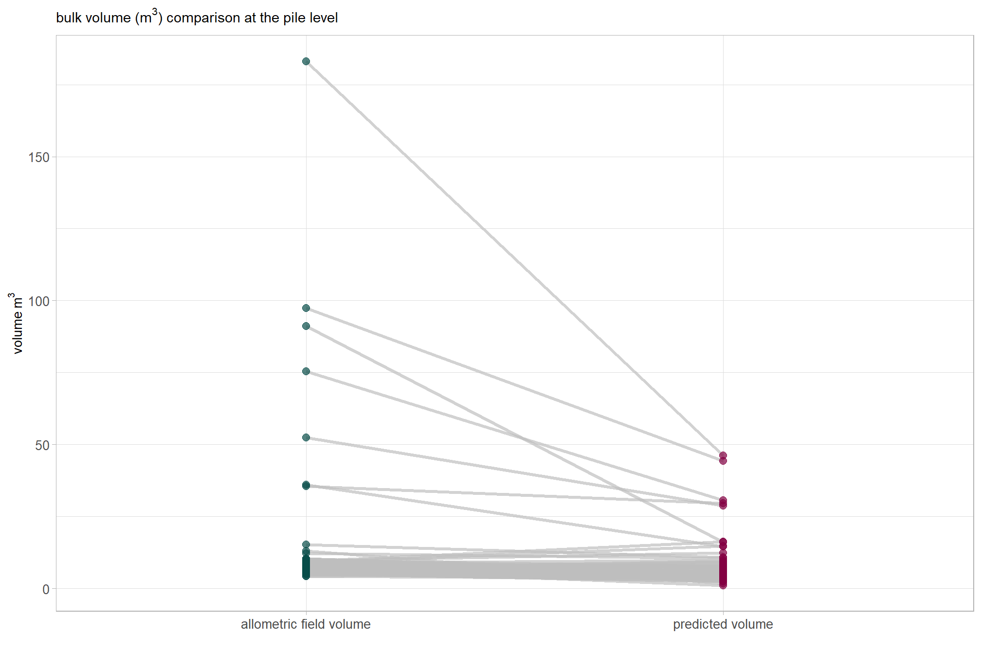
what if we only look at the smaller piles?
vol_df_temp %>%
  dplyr::filter(
    value < quantile(vol_df_temp$value, probs = 0.938)
  ) %>%
  ggplot2::ggplot(
    mapping = ggplot2::aes(x = name, y = value, group = pile_id)
  ) +
  ggplot2::geom_line(key_glyph = "point", alpha = 0.7, color = "gray", lwd = 1.1) +
  ggplot2::geom_point(mapping = ggplot2::aes(color = name), alpha = 0.7, size = 2.5) +
  harrypotter::scale_color_hp_d(option = "lunalovegood") +
  ggplot2::labs(
    color=""
    , y = latex2exp::TeX("volume $m^3$")
    , x = ""
    , subtitle = latex2exp::TeX("bulk volume ($m^3$) comparison at the pile level for the smaller piles")
  ) +
  ggplot2::theme_light() +
  ggplot2::theme(
    legend.position = "none"
    , axis.title = ggplot2::element_text(size = 10)
    , axis.text = ggplot2::element_text(size = 10)
  )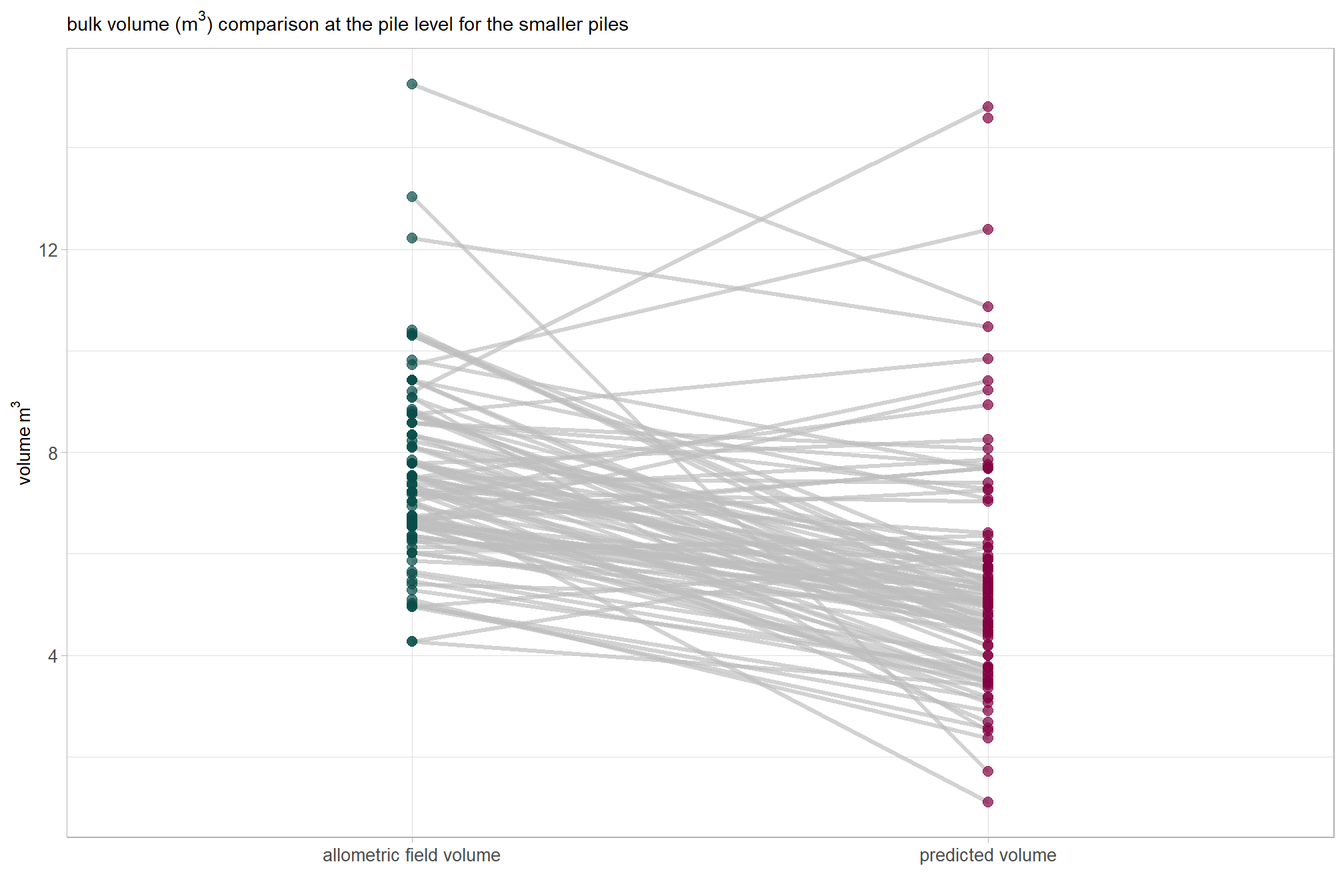
let’s compare aggregated volume measurements for the true positive matches
Mean Difference (MD): \[\text{MD} = \frac{1}{N} \sum_{i=1}^{N} (\text{Allometric Volume}_i - \text{Predicted Volume}_i)\]
Percent Mean Difference: \[\%\text{MD} = \frac{\text{MD}}{\text{Mean}(\text{Predicted Volume})} \times 100\]
vol_agg_df_temp <-
  ground_truth_prediction_match_ans %>%
  dplyr::filter(match_grp=="true positive") %>%
  dplyr::ungroup() %>%
  dplyr::summarise(
    mean_diff = mean(gt_volume_m3-pred_volume_m3)
    , sd_diff = sd(gt_volume_m3-pred_volume_m3)
    , mean_gt_volume_m3 = mean(gt_volume_m3,na.rm = T)
    , mean_pred_volume_m3 = mean(pred_volume_m3,na.rm = T)
  ) %>%
  dplyr::mutate(
    pct_mean_diff = mean_diff/mean_pred_volume_m3
  )
what did we get?
vol_agg_df_temp %>%
  tidyr::pivot_longer(dplyr::everything()) %>%
  dplyr::mutate(
    value =
      dplyr::case_when(
        stringr::str_starts(name, "pct_") ~ scales::percent(value, accuracy = 0.1)
        , T ~ scales::comma(value, accuracy = 0.1)
      )
  ) %>%
  kableExtra::kbl(
    caption = "comparison of aggregated allometric field volume and predicted volume"
    , col.names = c("metric", "value")
  ) %>%
kableExtra::kable_styling()| metric | value |
|---|---|
| mean_diff | 5.2 |
| sd_diff | 16.3 |
| mean_gt_volume_m3 | 12.4 |
| mean_pred_volume_m3 | 7.1 |
| pct_mean_diff | 73.4% |
we’ll dig into the MD shortly but before we move on let’s focus on the percent mean difference. We calcualted a %MD of 73.4% which indicates a major systematic difference where the allometric field volume is, on average, 73.4% larger than our CHM-predicted volume. This large relative difference shows how much the geometric assumptions inflate the volume compared to the irregular volumes measured by our remote sensing-based method.
let’s make a Bland-Altman plot to compare the two measurement methods. this plot uses the average of the two measurements (approximate size) on the x-axis and the difference (bias) between the two measurements on the y-axis
ground_truth_prediction_match_ans %>%
  dplyr::filter(match_grp=="true positive") %>%
  dplyr::ungroup() %>%
  # calc needed metrics
  dplyr::mutate(
    mean_vol = (gt_volume_m3+pred_volume_m3)/2
    , diff_vol = (gt_volume_m3-pred_volume_m3) # match the order used in vol_agg_df_temp
    , scale_diff = ifelse(diff_vol < 0, -abs(diff_vol) / abs(min(diff_vol)), diff_vol / max(diff_vol))
  ) %>%
  # ggplot() + geom_point(aes(x=diff_vol,y=0, color=scale_diff)) + scale_color_gradient2(mid = "gray", midpoint = 0, low = "red", high = "blue")
  # plot
  ggplot2::ggplot(
    mapping = ggplot2::aes(x = mean_vol, y = diff_vol)
  ) +
  ggplot2::geom_hline(yintercept = 0, color = "black", lwd = 1.2) +
  # mean difference (bias)
  ggplot2::geom_hline(
    yintercept = vol_agg_df_temp$mean_diff
    , linetype = "dashed", color = "blue", lwd = 1
  ) +
  # upper limit
  ggplot2::geom_hline(
    yintercept = vol_agg_df_temp$mean_diff+1.96*vol_agg_df_temp$sd_diff
    , linetype = "dotted", color = "red", lwd = 1
  ) +
  # lower limit
  ggplot2::geom_hline(
    yintercept = vol_agg_df_temp$mean_diff-1.96*vol_agg_df_temp$sd_diff
    , linetype = "dotted", color = "red", lwd = 1
  ) +
  # annotations
  ggplot2::annotate(
    "text"
    , x = Inf
    , y = vol_agg_df_temp$mean_diff
    , label = latex2exp::TeX(
      paste0(
        "mean difference (bias): "
        , scales::comma(vol_agg_df_temp$mean_diff, accuracy = 0.01)
        , " $m^3$"
      )
      , output = "character"
    )
    , vjust = -0.5
    , hjust = 1
    , color = "blue"
    , size = 4
    , parse = TRUE
  ) +
  ggplot2::annotate(
    "text"
    , x = Inf
    , y = vol_agg_df_temp$mean_diff+1.96*vol_agg_df_temp$sd_diff
    , label = latex2exp::TeX(
      paste0(
        "+1.96 SD: "
        , scales::comma(vol_agg_df_temp$mean_diff+1.96*vol_agg_df_temp$sd_diff, accuracy = 0.01)
        , " $m^3$"
      )
      , output = "character"
    )
    , vjust = -0.5
    , hjust = 1
    , color = "red"
    , size = 4
    , parse = TRUE
  ) +
  ggplot2::annotate(
    "text"
    , x = Inf
    , y = vol_agg_df_temp$mean_diff-1.96*vol_agg_df_temp$sd_diff
    , label = latex2exp::TeX(
      paste0(
        "-1.96 SD: "
        , scales::comma(vol_agg_df_temp$mean_diff-1.96*vol_agg_df_temp$sd_diff, accuracy = 0.01)
        , " $m^3$"
      )
      , output = "character"
    )
    , vjust = 1.5
    , hjust = 1
    , color = "red"
    , size = 4
    , parse = TRUE
  ) +
  # points
  ggplot2::geom_point(mapping = ggplot2::aes(color = scale_diff), size = 1.9, alpha = 0.8) +
  ggplot2::scale_color_steps2(mid = "gray", midpoint = 0) +
  ggplot2::labs(
    subtitle = "Bland-Altman plot: allometric field volume vs predicted volume"
    , x = latex2exp::TeX("mean volume ($m^3$)")
    , y = latex2exp::TeX("difference (allometric - predicted volume $m^3$)")
  ) +
  ggplot2::theme_light() +
  ggplot2::theme(legend.position = "none")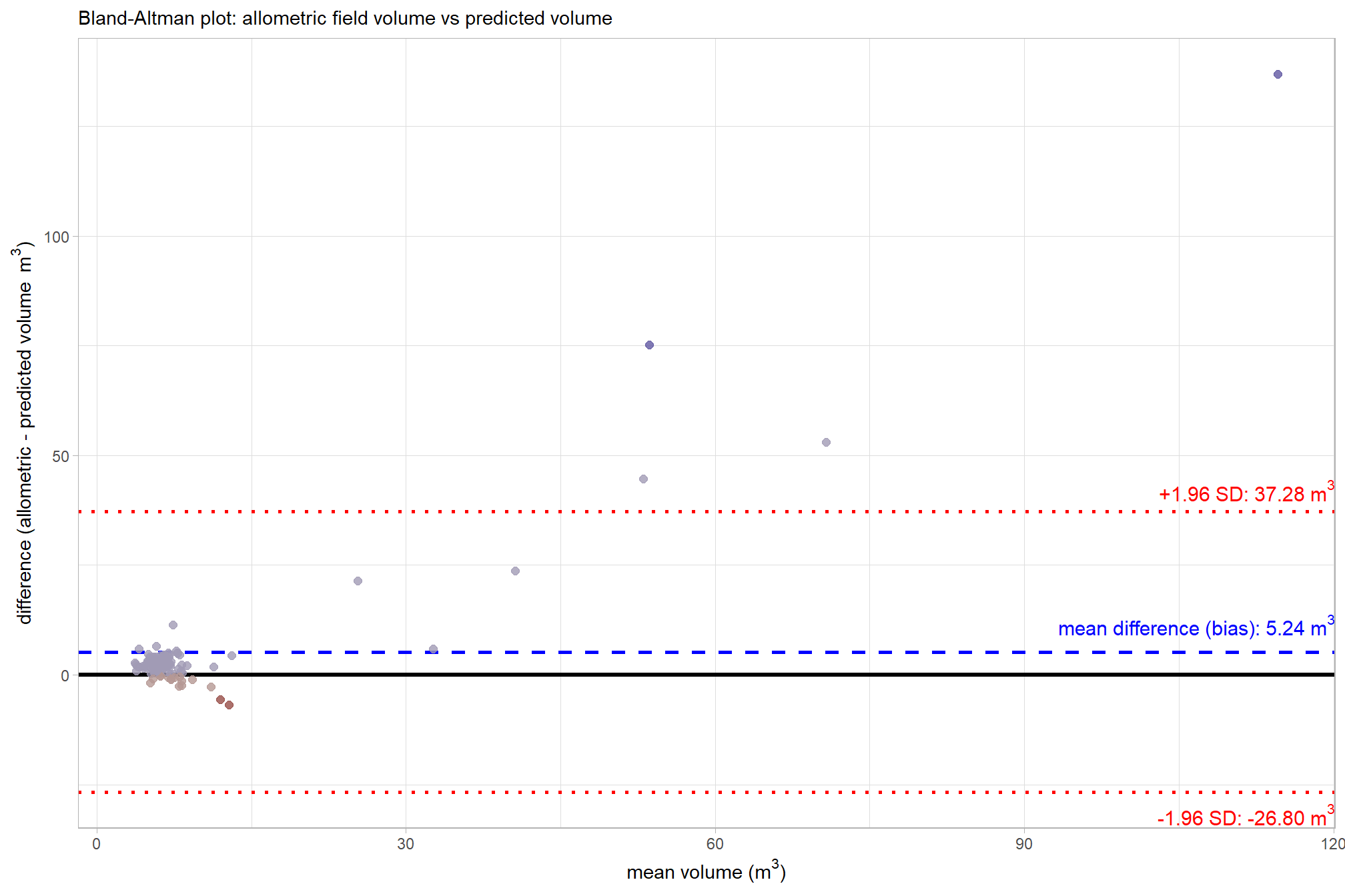
That’s a lot of plotting to show that the mean difference is 5.24 m3. Points falling outside the 95% interval on the plot are instances of significant disagreement between the two volume measurements for those specific data points. These outliers indicate that, for a particular pile, the difference between the allometric field volume and the predicted volume is unusually large, suggesting a potential failure in either the CHM segmentation process, the quality of the original field measurements, the geometric shape assumption, or a combination thereof. We should investigate these extreme disagreements further to see what is happening
before we do that, let’s use a paired t-test to determine if the mean difference (MD) between the allometric field volume and the predicted volume is statistically significant (i.e. significantly different from zero)
# is the mean difference between the two volumes significantly different from zero
ttest_temp <- t.test(
  ground_truth_prediction_match_ans %>%
    dplyr::filter(match_grp == "true positive") %>%
    dplyr::pull(gt_volume_m3)
  , ground_truth_prediction_match_ans %>%
    dplyr::filter(match_grp == "true positive") %>%
    dplyr::pull(pred_volume_m3)
  , paired = TRUE
)
ttest_temp
##
## Paired t-test
##
## data: ground_truth_prediction_match_ans %>% dplyr::filter(match_grp == "true positive") %>% dplyr::pull(gt_volume_m3) and ground_truth_prediction_match_ans %>% dplyr::filter(match_grp == "true positive") %>% dplyr::pull(pred_volume_m3)
## t = 3.3155, df = 106, p-value = 0.001253
## alternative hypothesis: true mean difference is not equal to 0
## 95 percent confidence interval:
## 2.106105 8.371658
## sample estimates:
## mean difference
## 5.238881that’s neat, the test gave us the same mean difference (MD) of 5.24 m3 that we calculated above. also, the p-value of 0.00125 is less than 0.05, meaning we should reject the null hypothesis that the true mean difference is zero. this confirms that the systematic difference (or bias) we observed where allometric volume is larger than our predicted volume is statistically significant and not due to random chance.
9.5.3.0.1 Extreme Volume Disagreements
let’s investigate the extreme disagreements further to see what is happening
bad_vol_df_temp <-
  ground_truth_prediction_match_ans %>%
  dplyr::filter(match_grp=="true positive") %>%
  dplyr::ungroup() %>%
  # calc needed metrics
  dplyr::mutate(
    diff_vol = (gt_volume_m3-pred_volume_m3) # match the order used in vol_agg_df_temp
  ) %>%
  dplyr::filter(
    diff_vol < (vol_agg_df_temp$mean_diff-1.96*vol_agg_df_temp$sd_diff)
    | diff_vol > (vol_agg_df_temp$mean_diff+1.96*vol_agg_df_temp$sd_diff)
  )
# what are the differences?
bad_vol_df_temp %>%
  dplyr::select(
    pile_id
    , gt_height_m, pred_height_m, diff_height_m
    , gt_diameter_m, pred_diameter_m, diff_field_diameter_m
    , gt_volume_m3, pred_volume_m3
  ) %>%
  dplyr::mutate(
    dplyr::across(
      .cols = -c(pile_id)
      , .fns = ~ scales::comma(.x,accuracy=0.01)
    )
  ) %>%
  kableExtra::kbl(
    caption = "Volume measurement outliers: comparison of ground truth and predicted piles"
    # , col.names = c("metric", "value")
  ) %>%
kableExtra::kable_styling()| pile_id | gt_height_m | pred_height_m | diff_height_m | gt_diameter_m | pred_diameter_m | diff_field_diameter_m | gt_volume_m3 | pred_volume_m3 |
|---|---|---|---|---|---|---|---|---|
| 194 | 6.40 | 2.30 | -4.10 | 8.53 | 8.48 | -0.06 | 183.08 | 46.12 |
| 82 | 4.27 | 2.30 | -1.97 | 7.62 | 7.56 | -0.06 | 97.30 | 44.24 |
| 76 | 4.72 | 1.73 | -2.99 | 7.01 | 5.68 | -1.33 | 91.18 | 16.01 |
| 8 | 4.27 | 2.30 | -1.97 | 6.71 | 7.38 | 0.67 | 75.35 | 30.69 |
smokes, it looks like the field-measured height is much different than the CHM height
bad_vol_df_temp %>%
  dplyr::select(
    pile_id
    , gt_height_m, pred_height_m
    , gt_diameter_m, pred_diameter_m
    , gt_volume_m3, pred_volume_m3
  ) %>%
  tidyr::pivot_longer(
    cols = -c(pile_id)
    , names_to = "metric"
    , values_to = "value"
  ) %>%
  dplyr::mutate(
    which_data = dplyr::case_when(
        stringr::str_starts(metric,"gt_") ~ "ground 'truth'"
        , stringr::str_starts(metric,"pred_") ~ "prediction"
        , T ~ "error"
      ) %>%
      ordered()
    , pile_metric = metric %>%
      stringr::str_remove("(_rmse|_rrmse|_mean|_mape)$") %>%
      stringr::str_extract("(paraboloid_volume|volume|area|height|diameter)") %>%
      factor(
        ordered = T
        , levels = c(
          "volume"
          , "paraboloid_volume"
          , "area"
          , "height"
          , "diameter"
        )
        , labels = c(
          "Volume (m3)"
          , "Volume paraboloid"
          , "Area (m2)"
          , "Height (m)"
          , "Diameter (m)"
        )
      )
  ) %>%
  ggplot2::ggplot(
    mapping = ggplot2::aes(x = which_data, y = value, label = scales::comma(value,accuracy=0.1), group = pile_id)
  ) +
  ggplot2::geom_line(key_glyph = "point", alpha = 0.7, color = "gray", lwd = 1.1) +
  ggplot2::geom_point(mapping = ggplot2::aes(color = which_data), alpha = 0.8, size = 2.5) +
  ggplot2::scale_color_manual(values = c("blue","brown")) +
  ggplot2::geom_text(
    vjust = -0.25
    , show.legend = FALSE
  ) +
  ggplot2::facet_grid(rows = dplyr::vars(pile_metric), scales = "free_y") +
  ggplot2::scale_y_continuous(labels = scales::comma, expand = ggplot2::expansion(mult = c(0.05,.32))) +
  ggplot2::labs(
    x = "", y = "", color = ""
    , subtitle = "Volume measurement outliers: comparison of measurements"
  ) +
  ggplot2::theme_light() +
  ggplot2::theme(
    legend.position = "none"
    , strip.text = ggplot2::element_text(size = 11, color = "black", face = "bold")
) 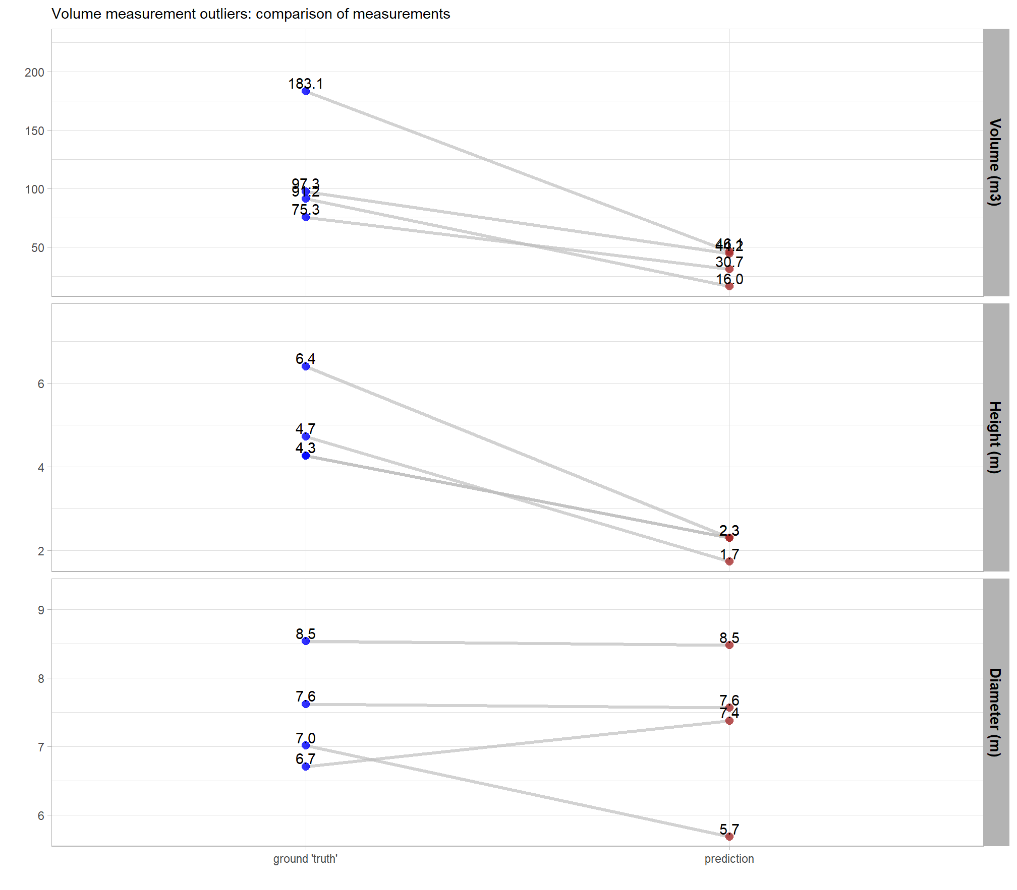
RGB with the predicted piles (brown) and the ground-truth piles (blue)
# plot RGB
plts_temp <-
  1:nrow(bad_vol_df_temp) %>%
  purrr::map(function(x){
    dta <- bad_vol_df_temp %>% dplyr::slice(x)
    gt <- slash_piles_polys %>% dplyr::filter(pile_id==dta$pile_id)
    pr <- final_predicted_slash_piles %>% dplyr::filter(pred_id==dta$pred_id)
    #plt
    ortho_plt_fn(my_ortho_rast=ortho_rast, stand=sf::st_union(gt,pr), buffer=6) +
      ggplot2::geom_sf(data = gt, fill = NA, color = "blue", lwd = 0.6) +
      ggplot2::geom_sf(data = pr, fill = NA, color = "brown", lwd = 0.5)
  })
# combine
patchwork::wrap_plots(
  plts_temp
  , ncol = 2
)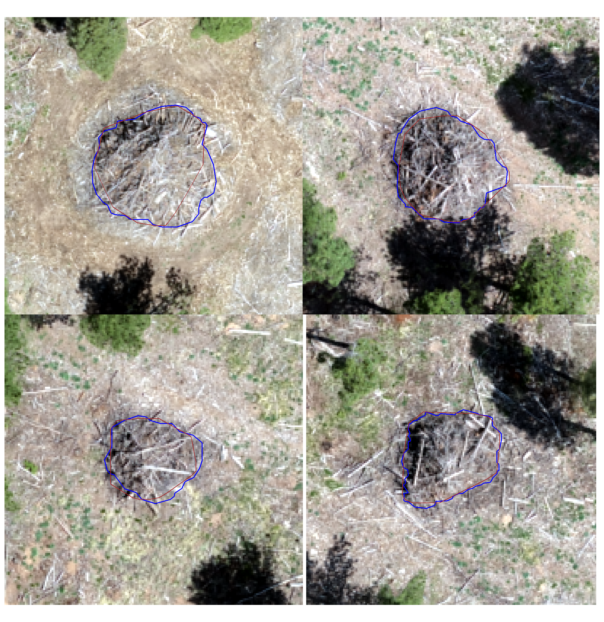
just looking at the RGB, the pile footprints are in good alignment
let’s look at the CHM
# cloud2raster_ans$chm_rast %>%
#   terra::clamp(upper = structural_params_settings$max_ht_m, lower = 0, values = F) %>%
#   terra::plot()
# bad_vol_df_temp %>% dplyr::glimpse()
# plot RGB + CHM
plts_temp <-
  1:nrow(bad_vol_df_temp) %>%
  # sample(1) %>%
  purrr::map(function(x){
    dta <- bad_vol_df_temp %>% dplyr::slice(x)
    gt <- slash_piles_polys %>% dplyr::filter(pile_id==dta$pile_id)
    pr <- final_predicted_slash_piles %>% dplyr::filter(pred_id==dta$pred_id)
    #plt
    ortho_plt_fn(my_ortho_rast=ortho_rast, stand=sf::st_union(gt,pr), buffer=6) +
      ggplot2::geom_tile(
        data = cloud2raster_ans$chm_rast %>%
          terra::crop(
            sf::st_union(gt,pr) %>%
              sf::st_transform(terra::crs(cloud2raster_ans$chm_rast)) %>%
              terra::vect()
          ) %>%
          terra::mask(
            sf::st_union(gt,pr) %>%
              sf::st_transform(terra::crs(cloud2raster_ans$chm_rast)) %>%
              terra::vect()
          ) %>%
          # slice the chm below our desired height
          # this is what slash_pile_detect_watershed() does
          terra::clamp(upper = structural_params_settings$max_ht_m, lower = 0, values = F) %>%
          terra::as.data.frame(xy=T) %>%
          dplyr::rename(f=3)
        , mapping = ggplot2::aes(x=x,y=y,fill=f)
        , alpha = 0.5
      ) +
      ggplot2::scale_fill_viridis_c(option = "plasma", na.value = "gray",name = "CHM (m)") +
      ggplot2::geom_sf(data = gt, fill = NA, color = "blue", lwd = 0.6) +
      ggplot2::geom_sf(data = pr, fill = NA, color = "brown", lwd = 0.5) +
      ggplot2::labs(
        subtitle = paste0(
          "GT ht: ", round(dta$gt_height_m,1)
          , " | Pred ht: ", round(dta$pred_height_m,1)
          , "\nGT dia: ", round(dta$gt_diameter_m,1)
          , " | Pred dia: ", round(dta$pred_diameter_m,1)
        )
      ) +
      ggplot2::theme(legend.text = ggplot2::element_text(size = 6),legend.title = ggplot2::element_text(size = 6))
  })
# plts_temp
# combine
patchwork::wrap_plots(
  plts_temp
  , ncol = 2
)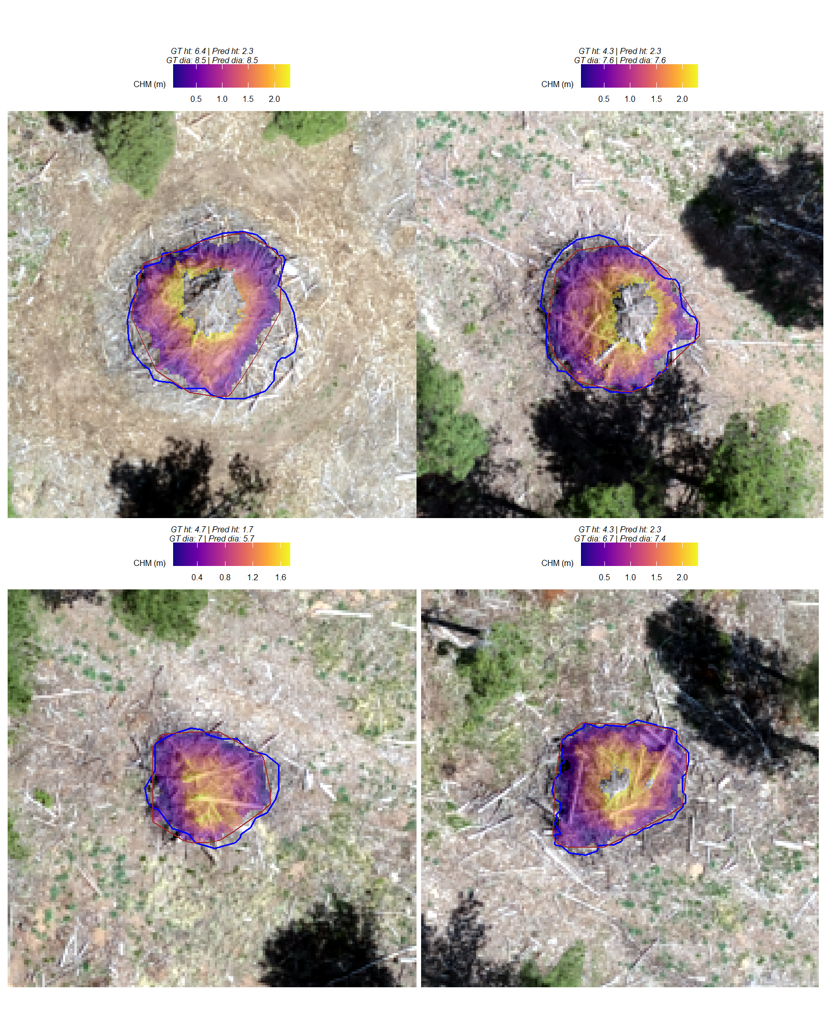
The predicted diameters generally align well with the field-measured diameters. However, the field-measured heights for some piles appear unusually high compared to the CHM-derived data.
Our pile detection methodology uses a specific height slice of the CHM based on the max_ht_m parameter. This process then keeps only predicted piles that meet the height threshold across the majority of their area. The convexity_pct parameter functions to filter out predictions where excessive pile top area was removed by the CHM slicing and acts as a safeguard against misclassifying tall objects (like trees) as piles that would have the majority of their top removed by the slicing.
After filtering for expected height, our detection methodology calculates the predicted height as the maximum CHM cell value within the expected height range (i.e. up to the max_ht_m setting), which effectively caps any actual height values above this threshold. For our training data, we assumed a maximum height of 2.30m. The field data contains heights up to 6.40m for these volume outliers, which would only be expected of the largest machine piles. In these extreme cases, the significant volume difference observed in the outliers is magnified by both potentially incorrect field measurements and the systematic capping of the predicted height.
To mitigate the risk of vastly underpredicted heights for these tall outliers, one can increase the convexity_pct parameter. Making this filtering more strict will remove the outlier height predictions and improve height quantification accuracy for true positive matches, but will likely reduce the detection rate as these piles become false negatives (omissions). Alternatively, one could increase the max_ht_m setting to be less restrictive with the height filtering; this would have the effect of estimating a more accurate height value for these tall piles but would potentially introduce new false positive predictions that are actually trees (or yurts?). If spectral data is available to filter these after structural segmentation, then this might be the preferred path to improve height quantification accuracy while maintaining detection accuracy. The choice ultimately depends on whether the user prioritizes detection rate or height quantification accuracy.
There is precedent for smoothing the height of piles from aerial data point cloud data. Trofymow et al. (2013) calculated pile height as the 95th percentile height of the height-normalized points within the pile polygon. This method was chosen after their preliminary analysis showed it best excluded points from isolated logs extending above the pile while retaining the main pile structure. Our method achieves a functionally similar result for the largest piles by capping the maximum CHM value and smoothing out extreme height measurements.
we can look a the full CHM without capping the height to see how the field-measured values compare to the unfiltered CHM height profile within the pile footprint
# cloud2raster_ans$chm_rast %>%
#   terra::clamp(upper = structural_params_settings$max_ht_m, lower = 0, values = F) %>%
#   terra::plot()
# bad_vol_df_temp %>% dplyr::glimpse()
# plot RGB + CHM
plts_temp <-
  1:nrow(bad_vol_df_temp) %>%
  # sample(1) %>%
  purrr::map(function(x){
    dta <- bad_vol_df_temp %>% dplyr::slice(x)
    gt <- slash_piles_polys %>% dplyr::filter(pile_id==dta$pile_id)
    pr <- final_predicted_slash_piles %>% dplyr::filter(pred_id==dta$pred_id)
    #plt
    ortho_plt_fn(my_ortho_rast=ortho_rast, stand=sf::st_union(gt,pr), buffer=6) +
      ggplot2::geom_tile(
        data = cloud2raster_ans$chm_rast %>%
          terra::crop(
            sf::st_union(gt,pr) %>%
              sf::st_transform(terra::crs(cloud2raster_ans$chm_rast)) %>%
              terra::vect()
          ) %>%
          terra::mask(
            sf::st_union(gt,pr) %>%
              sf::st_transform(terra::crs(cloud2raster_ans$chm_rast)) %>%
              terra::vect()
          ) %>%
          # DON'T slice the chm below our desired height
          # terra::clamp(upper = structural_params_settings$max_ht_m, lower = 0, values = F) %>%
          terra::as.data.frame(xy=T) %>%
          dplyr::rename(f=3)
        , mapping = ggplot2::aes(x=x,y=y,fill=f)
        , alpha = 0.5
      ) +
      ggplot2::scale_fill_viridis_c(option = "plasma", na.value = "gray",name = "CHM (m)", breaks = scales::breaks_extended(n=7)) +
      ggplot2::geom_sf(data = gt, fill = NA, color = "blue", lwd = 0.6) +
      ggplot2::geom_sf(data = pr, fill = NA, color = "brown", lwd = 0.5) +
      ggplot2::labs(
        subtitle = paste0(
          "GT ht: ", round(dta$gt_height_m,1)
          , " | Pred ht: ", round(dta$pred_height_m,1)
          , "\nGT dia: ", round(dta$gt_diameter_m,1)
          , " | Pred dia: ", round(dta$pred_diameter_m,1)
        )
      ) +
      ggplot2::theme(legend.text = ggplot2::element_text(size = 6),legend.title = ggplot2::element_text(size = 6))
  })
# plts_temp
# combine
patchwork::wrap_plots(
  plts_temp
  , ncol = 2
)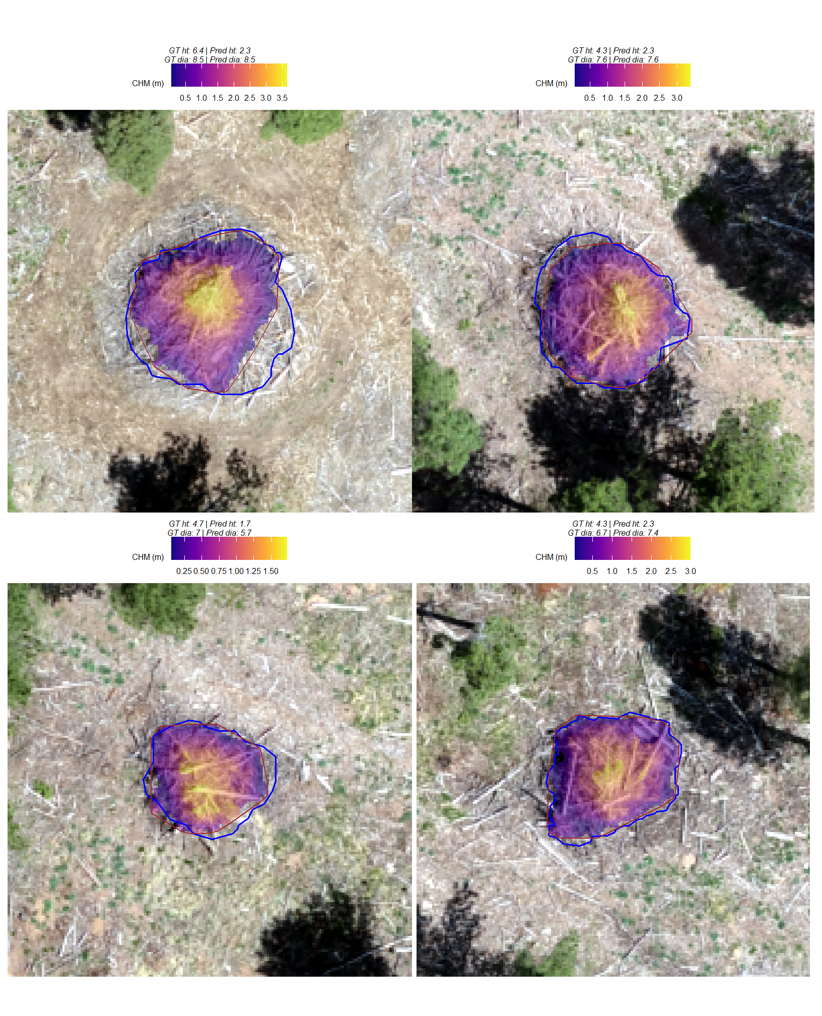
Visual inspection of the unfiltered CHM (note the CHM scale range) within the footprint of these volume outliers confirms that the field-measured values are misaligned with the CHM profile by at least 1m for some of the most extreme outliers, supporting the theory that the significant volume and height differences observed are magnified by potentially incorrect field measurements.
9.5.4 Stand-level Aggregation
before we leave, let’s summarize the measurement values of the predictions (true positive and false positive) and the ground truth data (true positive and false negative) over the entire stand (this is similar to a basal area comparison in a forest inventory)
sum_df_temp <-
  ground_truth_prediction_match_ans %>%
  dplyr::ungroup() %>%
  dplyr::select(-c(pred_id)) %>%
  dplyr::summarise(
    dplyr::across(
      .cols = tidyselect::starts_with("gt_") | tidyselect::starts_with("pred_")
      , ~sum(.x,na.rm=T)
    )
  ) %>%
  tidyr::pivot_longer(
    cols = dplyr::everything()
    , names_to = "metric"
    , values_to = "value"
  ) %>%
  dplyr::mutate(
    which_data = dplyr::case_when(
        stringr::str_starts(metric,"gt_") ~ "ground truth"
        , stringr::str_starts(metric,"pred_") ~ "prediction"
        , T ~ "error"
      ) %>%
      ordered()
    , pile_metric = metric %>%
      stringr::str_remove("(_rmse|_rrmse|_mean|_mape)$") %>%
      stringr::str_extract("(paraboloid_volume|volume|area|height|diameter)") %>%
      factor(
        ordered = T
        , levels = c(
          "height"
          , "diameter"
          , "area"
          , "volume"
          , "paraboloid_volume"
        )
        , labels = c(
          "Height (m)"
          , "Diameter (m)"
          , "Area (m2)"
          , "Volume (m3)"
          , "Volume paraboloid"
        )
      )
  ) %>%
  dplyr::group_by(pile_metric) %>%
  dplyr::arrange(pile_metric,which_data) %>%
  dplyr::mutate(
    pct_diff = (value-dplyr::lag(value))/dplyr::lag(value)
  ) %>%
  dplyr::ungroup()
plot
# plot it
sum_df_temp %>%
  dplyr::ungroup() %>%
  dplyr::mutate(
    stand_id=1
    , lab = paste0(
      scales::comma(value,accuracy=0.1)
      , dplyr::case_when(
        is.na(pct_diff) ~ ""
        , T ~ paste0(
          "\n"
          , ifelse(pct_diff<0,"-","+")
          ,scales::percent(abs(pct_diff),accuracy=0.1)
        )
      )
    )
  ) %>%
  ggplot2::ggplot(
    mapping = ggplot2::aes(
      x = which_data
      , y = value
      , label = lab
      , group = stand_id
    )
  ) +
  ggplot2::geom_line(key_glyph = "point", alpha = 0.7, color = "gray", lwd = 1.1) +
  ggplot2::geom_col(mapping = ggplot2::aes(fill = which_data), alpha = 1, width = 0.4) +
  ggplot2::scale_color_manual(values = c("blue","brown")) +
  ggplot2::scale_fill_manual(values = c("blue","brown")) +
  ggplot2::geom_text(
    vjust = -0.25
  ) +
  ggplot2::facet_grid(rows = dplyr::vars(pile_metric), scales = "free_y", axes = "all_x") +
  ggplot2::scale_y_continuous(labels = scales::comma, expand = ggplot2::expansion(mult = c(0,.3)), breaks = NULL) +
  ggplot2::labs(
    x = "", y = "", color = ""
    , subtitle = "Comparison of aggregated measurements at the stand level"
  ) +
  ggplot2::theme_light() +
  ggplot2::theme(
    legend.position = "none"
    , axis.text.x = ggplot2::element_text(size = 11, color = "black", face = "bold")
    , strip.text = ggplot2::element_text(size = 11, color = "black", face = "bold")
    , panel.grid = ggplot2::element_blank()
) 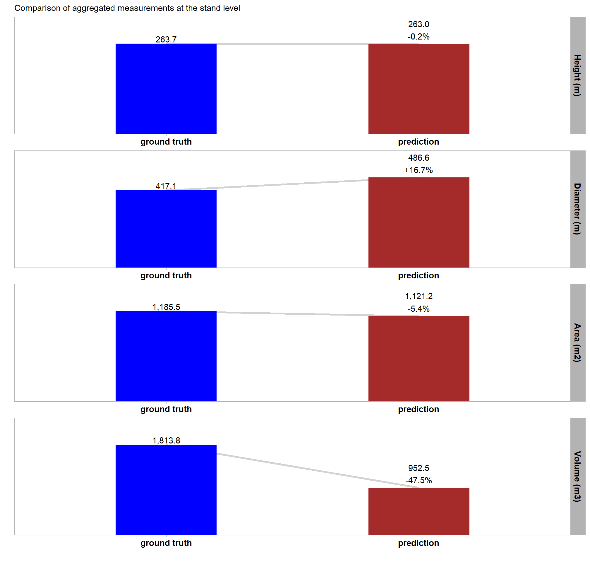
table it
sum_df_temp %>%
  dplyr::select(pile_metric, which_data, value, pct_diff) %>%
  dplyr::mutate(
    value = scales::comma(value,accuracy=0.1)
    , pct_diff = scales::percent(pct_diff,accuracy=0.1)
  ) %>%
  kableExtra::kbl(
    caption = "Comparison of aggregated measurements at the stand level"
    , col.names = c(
      ".", "measurement source"
      , "stand-level total", "% difference"
    )
    , escape = F
  ) %>%
  kableExtra::kable_styling() %>%
kableExtra::collapse_rows(columns = 1, valign = "top")| . | measurement source | stand-level total | % difference |
|---|---|---|---|
| Height (m) | ground truth | 263.7 | NA |
| prediction | 263.0 | -0.2% | |
| Diameter (m) | ground truth | 417.1 | NA |
| prediction | 486.6 | 16.7% | |
| Area (m2) | ground truth | 1,185.5 | NA |
| prediction | 1,121.2 | -5.4% | |
| Volume (m3) | ground truth | 1,813.8 | NA |
| prediction | 952.5 | -47.5% |