Section 8 Sensitivity Testing Results
In this section we’ll use the slash pile detection workflow to perform parameter sensitivity testing with different resolution CHM data as input. The objective here is to generate the point estimate data for statistical analysis to fully evaluate our slash pile detection method’s performance. In this prior section, we demonstrated how to use the cloud2trees::cloud2raster() function to process raw point cloud data CHM data (a DSM with the ground removed) for our raster-based watershed segmentation methodology. The cloud2trees package makes it easy to generate CHM data at various resolutions, so we’ll use it to systematically test the influence of CHM resolution on both pile detection and form quantification accuracy. Using various CHM resolutions, we will repeatedly execute the entire pile detection method while systematically varying the values of one or more structural parameters (such as minimum area or maximum height). These sensitivity tests will be performed under two conditions: using only the CHM data as input (structural detection) and incorporating the RGB spectral data via our data fusion approach across five different levels of the spectral_weight parameter. The results of these sensitivity tests will serve as individual point estimates of detection accuracy (i.e. F-score) and quantification accuracy (e.g., RMSE and MAPE) for each unique combination of CHM resolution, spectral data weighting, and parameter settings. This generated dataset will be used as the input for subsequent statistical modeling to quantify the influence of parameters and input data on the detection and form quantification accuracy of our slash pile detection methodology.
8.1 Process Raw Point Cloud
We’ll use cloud2trees::cloud2raster() to process the raw point cloud data to generate a set of CHM rasters at varying resolutions
chm_res_list <- seq(from=0.10,to=0.50,by=0.1)
# process point clouds
chm_res_list %>%
  purrr::map(function(chm_res_m){
    message(paste0("CHMing...........",chm_res_m))
    dir_temp <- paste0("../data/point_cloud_processing_delivery_chm",chm_res_m,"m")
    # do it
    if(!dir.exists(dir_temp)){
      # cloud2trees
      cloud2raster_ans <- cloud2trees::cloud2raster(
        output_dir = "../data"
        , input_las_dir = "f:\\PFDP_Data\\p4pro_images\\P4Pro_06_17_2021_half_half_optimal\\2_densification\\point_cloud"
        , accuracy_level = 2
        , keep_intrmdt = T
        , dtm_res_m = 0.25
        , chm_res_m = chm_res_m
        , min_height = 0 # effectively generates a DSM based on non-ground points
      )
      # rename
      file.rename(from = "../data/point_cloud_processing_delivery", to = dir_temp)
    }
  })
# which dirs?
chm_res_list[
  chm_res_list %>%
    purrr::map(~paste0("../data/point_cloud_processing_delivery_chm",.x,"m")) %>%
    unlist() %>%
    dir.exists()
]
8.2 Structural Only: Parameter Testing
we could simply map these combinations over our slash_pile_detect_watershed() function we reviewed in this prior section, but that would entail performing the same action multiple times. we defined a specialized function to efficiently map over all of these combinations in this section to obtain pile predictions based on the different settings.
let’s test different parameter combinations of our watershed segmentation, rules-based slash pile detection methodology for each CHM raster resolution from more coarse, to finer resolution
param_combos_df <-
  tidyr::crossing(
    max_ht_m = seq(from = 2, to =  5, by = 1) # set the max expected pile height (could also do a minimum??)
    , min_area_m2 = c(2) # seq(from = 1, to =  2, by = 1) # set the min expected pile area
    , max_area_m2 = seq(from = 10, to = 60, by = 10) # set the max expected pile area
    , convexity_pct = seq(from = 0.05, to = 0.95, length.out = 7) # min required overlap between the predicted pile and the convex hull of the predicted pile
    , circle_fit_iou_pct = seq(from = 0.05, to = 0.95, length.out = 7)
  ) %>%
  dplyr::mutate(rn = dplyr::row_number()) %>%
  dplyr::relocate(rn)
# param_combos_df %>% dplyr::glimpse()
# param_combos_df %>% dplyr::count(convexity_pct)
# param_combos_df %>% dplyr::count(circle_fit_iou_pct)
# seq(from = 0.05, to = 0.95, length.out = 7)

# how many combos are we testing?
n_combos_tested_chm <- nrow(param_combos_df) #combos per chm
n_combos_tested <- length(chm_res_list)*n_combos_tested_chm #combos overall structural only
# there are 5 spectral_weight settings + no spectral data (spectral_weight=0) = 6
spectral_settings_tested <- 6
# how many combos overall is this for the spectral testing?
n_combos_tested_spectral <- n_combos_tested*spectral_settings_tested
# how many combos PER CHM is this for the spectral testing?
n_combos_tested_spectral_chm <- n_combos_tested_chm*spectral_settings_tested
map over each CHM raster for pile detection using each of these parameter combinations
param_combos_piles_flist <- chm_res_list %>%
  purrr::map(function(chm_res_m){
    message(paste0("param_combos_piles_detect_fn...........",chm_res_m))
    # file
    f_temp <- file.path("../data",paste0("param_combos_piles_chm",chm_res_m,"m.gpkg"))
    # chm dir
    dir_temp <- paste0("../data/point_cloud_processing_delivery_chm",chm_res_m,"m")
    # chm file
    chm_f <- file.path(dir_temp, paste0("chm_", chm_res_m,"m.tif"))
    # check and do it
    if(!file.exists(f_temp) && file.exists(chm_f) ){
      # read chm
      chm_rast <- terra::rast(chm_f)
      # do it
      param_combos_piles <- param_combos_piles_detect_fn(
        chm = chm_rast %>%
          terra::crop(
            stand_boundary %>%
              dplyr::slice(1) %>%
              sf::st_buffer(5) %>%
              sf::st_transform(terra::crs(chm_rast)) %>%
              terra::vect()
          )
        , param_combos_df = param_combos_df
        , smooth_segs = T
        , ofile = f_temp
      )
      # param_combos_piles %>% dplyr::glimpse()

      # save it
      sf::st_write(param_combos_piles, f_temp, append = F, quiet = T)
      return(f_temp)
    }else if(file.exists(f_temp)){
      return(f_temp)
    }else{
      return(NULL)
    }
  })
# which successes?
param_combos_piles_flist
8.2.1 Validation over parameter combinations
now we need to validate these combinations against the ground truth data and we can map over the ground_truth_prediction_match() function to get true positive, false positive (commission), and false negative (omission) classifications for the predicted and ground truth piles
param_combos_gt_flist <- chm_res_list %>%
  purrr::map(function(chm_res_m){
    message(paste0("ground_truth_prediction_match...........",chm_res_m))
    param_combos_piles_fnm <- file.path("../data",paste0("param_combos_piles_chm",chm_res_m,"m.gpkg"))
    # file creating now
    f_temp <- file.path("../data",paste0("param_combos_gt_chm",chm_res_m,"m.csv"))
    # check
    if(!file.exists(f_temp) && file.exists(param_combos_piles_fnm)){
      # read it
      param_combos_piles <- sf::st_read(param_combos_piles_fnm)
      # do it
      param_combos_gt <-
        unique(param_combos_df$rn) %>%
        purrr::map(\(x)
          ground_truth_prediction_match(
            ground_truth = slash_piles_polys %>%
              dplyr::filter(is_in_stand) %>%
              dplyr::arrange(desc(field_diameter_m)) %>%
              sf::st_transform(sf::st_crs(param_combos_piles))
            , gt_id = "pile_id"
            , predictions = param_combos_piles %>%
              dplyr::filter(rn == x) %>%
              dplyr::filter(
                pred_id %in% (param_combos_piles %>%
                  dplyr::filter(rn == x) %>%
                  sf::st_intersection(
                    stand_boundary %>%
                      sf::st_transform(sf::st_crs(param_combos_piles))
                  ) %>%
                  sf::st_drop_geometry() %>%
                  dplyr::pull(pred_id))
              )
            , pred_id = "pred_id"
            , min_iou_pct = 0.05
          ) %>%
          dplyr::mutate(rn=x)
        ) %>%
        dplyr::bind_rows()
      # write it
      param_combos_gt %>% readr::write_csv(f_temp, append = F, progress = F)
      return(f_temp)
    }else if(file.exists(f_temp)){
      return(f_temp)
    }else{
      return(NULL)
    }
  })
# which successes?
param_combos_gt_flist
8.2.2 Aggregate Validation Metrics to Parameter Combination
now we’re going to calculate aggregated detection accuracy metrics and quantification accuracy metrics
detection accuracy metrics:
- Precision precision measures how many of the objects our method detected as slash piles were actually correct. A high precision means the method has a low rate of false alarms.
- Recall recall (i.e. detection rate) indicates how many actual (ground truth) slash piles our method successfully identified. High recall means the method is good at finding most existing piles, minimizing omissions.
- F-score provides a single, balanced measure that combines both precision and recall. A high F-score indicates overall effectiveness in both finding most piles and ensuring most detections are correct.
quantification accuracy metrics:
- Mean Error (ME) represents the direction of bias (over or under-prediction) in the original units
- RMSE represents the typical magnitude of error in the original units, with a stronger penalty for large errors
- MAPE represents the typical magnitude of error as a percentage, allowing for scale-independent comparisons
regarding the form quantification accuracy evaluation, we will assess the method’s accuracy by comparing the true-positive matches using the following metrics:
- Diameter compares the predicted diameter (from the maximum internal distance) to the ground truth field-measured diameter
- Area compares the predicted area from the irregular shape to the image-annotated area based on the potentially irregular pile perimeter
- Height compares the predicted maximum height from the CHM to the ground truth field-measured height
param_combos_gt_agg_flist <- chm_res_list %>%
  purrr::map(function(chm_res_m){
    message(paste0("param_combos_gt_agg...........",chm_res_m))
    # param_combos_piles file
    param_combos_piles_fnm <- param_combos_piles_flist %>% stringr::str_subset(pattern = paste0("chm",chm_res_m,"m.gpkg")) %>% purrr::pluck(1)
    if(is.null(param_combos_piles_fnm) || !file.exists(param_combos_piles_fnm)){return(NULL)}
    # param_combos_gt file
    param_combos_gt_fnm <- param_combos_gt_flist %>% stringr::str_subset(pattern = paste0("chm",chm_res_m,"m.csv")) %>% purrr::pluck(1)
    if(is.null(param_combos_gt_fnm) || !file.exists(param_combos_gt_fnm)){return(NULL)}
    # file creating now
    f_temp <- file.path("../data",paste0("param_combos_gt_agg_chm",chm_res_m,"m.csv"))
    # check and do it
    if(!file.exists(f_temp)){
      # read param_combos_piles
      param_combos_piles <- sf::st_read(param_combos_piles_fnm)
      # read param_combos_piles
      param_combos_gt <- readr::read_csv(param_combos_gt_fnm)

      #######################################
      # let's attach a flag to only work with piles that intersect with the stand boundary
      # add in/out to piles data
      #######################################
      param_combos_piles <- param_combos_piles %>%
        dplyr::left_join(
          param_combos_piles %>%
            sf::st_intersection(
              stand_boundary %>%
                sf::st_transform(sf::st_crs(param_combos_piles))
            ) %>%
            sf::st_drop_geometry() %>%
            dplyr::select(rn,pred_id) %>%
            dplyr::mutate(is_in_stand = T)
          , by = dplyr::join_by(rn,pred_id)
        ) %>%
        dplyr::mutate(
          is_in_stand = dplyr::coalesce(is_in_stand,F)
        ) %>%
        # # get the length (diameter) and width of the polygon
        # st_bbox_by_row(dimensions = T) %>% # gets shape_length, where shape_length=length of longest bbox side
        # and paraboloid volume
        dplyr::mutate(
          # paraboloid_volume_m3 = (1/8) * pi * (shape_length^2) * max_height_m
          paraboloid_volume_m3 = (1/8) * pi * (diameter_m^2) * max_height_m
        )
      # param_combos_piles %>% dplyr::glimpse()
      #######################################
      # add data to validation
      #######################################
      param_combos_gt <-
        param_combos_gt %>%
        dplyr::mutate(pile_id = as.numeric(pile_id)) %>%
        # add area of gt
        dplyr::left_join(
          slash_piles_polys %>%
            sf::st_drop_geometry() %>%
            dplyr::select(pile_id,image_gt_area_m2,height_m,field_diameter_m) %>%
            dplyr::rename(
              gt_height_m = height_m
              , gt_diameter_m = field_diameter_m
              , gt_area_m2 = image_gt_area_m2
            ) %>%
            dplyr::mutate(pile_id=as.numeric(pile_id))
          , by = "pile_id"
        ) %>%
        # add info from predictions
        dplyr::left_join(
          param_combos_piles %>%
            sf::st_drop_geometry() %>%
            dplyr::select(
              rn,pred_id
              , is_in_stand
              , area_m2, volume_m3, max_height_m, diameter_m
              , paraboloid_volume_m3
              # , shape_length # , shape_width
            ) %>%
            dplyr::rename(
              pred_area_m2 = area_m2, pred_volume_m3 = volume_m3
              , pred_height_m = max_height_m, pred_diameter_m = diameter_m
              , pred_paraboloid_volume_m3 = paraboloid_volume_m3
            )
          , by = dplyr::join_by(rn,pred_id)
        ) %>%
        dplyr::mutate(
          is_in_stand = dplyr::case_when(
            is_in_stand == T ~ T
            , is_in_stand == F ~ F
            , match_grp == "omission" ~ T
            , T ~ F
          )
          ### calculate these based on the formulas below...agg_ground_truth_match() depends on those formulas
          # area_m2
          , diff_area_m2 = pred_area_m2-gt_area_m2
          , pct_diff_area_m2 = (gt_area_m2-pred_area_m2)/gt_area_m2
          # height_m
          , diff_height_m = pred_height_m-gt_height_m
          , pct_diff_height_m = (gt_height_m-pred_height_m)/gt_height_m
          # diameter_m
          , diff_diameter_m = pred_diameter_m-gt_diameter_m
          , pct_diff_diameter_m = (gt_diameter_m-pred_diameter_m)/gt_diameter_m
        )
      #######################################
      # aggregate results from ground_truth_prediction_match()
      #######################################
      param_combos_gt_agg <- unique(param_combos_gt$rn) %>%
        purrr::map(\(x)
          agg_ground_truth_match(
            param_combos_gt %>%
              dplyr::filter(
                is_in_stand
                & rn == x
              )
          ) %>%
          dplyr::mutate(rn = x) %>%
          dplyr::select(!tidyselect::starts_with("gt_"))
        ) %>%
        dplyr::bind_rows() %>%
        # add in info on all parameter combinations
        dplyr::inner_join(
          param_combos_piles %>%
          sf::st_drop_geometry() %>%
          dplyr::distinct(
            rn,max_ht_m,min_area_m2,max_area_m2,convexity_pct,circle_fit_iou_pct
          )
          , by = "rn"
          , relationship = "one-to-one"
        )
      # write it
      param_combos_gt_agg %>% readr::write_csv(f_temp, append = F, progress = F)
      return(f_temp)
    }else if(file.exists(f_temp)){
      return(f_temp)
    }else{
      return(NULL)
    }
  })
# which successes?
param_combos_gt_agg_flist
8.3 Data Fusion: Parameter Testing
We also reviewed a data fusion approach that uses both a CHM generated from aerial point cloud data (for structural information) and RGB imagery, whereby initial candidate slash piles are first identified based on their structural form and then, filtered spectrally using the RGB imagery. We created a process to perform this filtering which takes as input: 1) a spatial data frame of candidate polygons; 2) a raster with RGB spectral data; 3) user-defined spectral weighting (voting system). let’s apply that process to the candidate piles detected using the structural data only from the prior section.
param_combos_spectral_gt_flist <- chm_res_list %>%
  purrr::map(function(chm_res_m){
    message(paste0("param_combos_spectral_gt...........",chm_res_m))
    # param_combos_piles file
    param_combos_piles_fnm <- param_combos_piles_flist %>% stringr::str_subset(pattern = paste0("chm",chm_res_m,"m.gpkg")) %>% purrr::pluck(1)
    if(is.null(param_combos_piles_fnm) || !file.exists(param_combos_piles_fnm)){return(NULL)}
    # param_combos_gt file
    param_combos_gt_fnm <- param_combos_gt_flist %>% stringr::str_subset(pattern = paste0("chm",chm_res_m,"m.csv")) %>% purrr::pluck(1)
    if(is.null(param_combos_gt_fnm) || !file.exists(param_combos_gt_fnm)){return(NULL)}
    # file creating now
    f_temp <- file.path("../data",paste0("param_combos_spectral_gt_chm",chm_res_m,"m.csv"))
    # check and do it
    if(!file.exists(f_temp)){
      # read param_combos_piles
      param_combos_piles <- sf::st_read(param_combos_piles_fnm)
      # read param_combos_piles
      param_combos_gt <- readr::read_csv(param_combos_gt_fnm)

      #######################################
      # let's attach a flag to only work with piles that intersect with the stand boundary
      # add in/out to piles data
      #######################################
      param_combos_spectral_gt <-
        c(1:5) %>%
        purrr::map(function(sw){
          # polygon_spectral_filtering
          param_combos_piles_filtered <- polygon_spectral_filtering(
              sf_data = param_combos_piles
              , rgb_rast = ortho_rast
              , red_band_idx = 1
              , green_band_idx = 2
              , blue_band_idx = 3
              , spectral_weight = sw
            ) %>%
            dplyr::mutate(spectral_weight=sw)

          # dplyr::glimpse(param_combos_piles_filtered)
          # param_combos_piles_filtered %>% sf::st_drop_geometry() %>% dplyr::count(rn) %>%
          #   dplyr::inner_join(
          #     param_combos_piles %>% sf::st_drop_geometry() %>% dplyr::count(rn) %>% dplyr::rename(orig_n=n)
          #   ) %>%
          #   dplyr::arrange(desc(orig_n-n))

          # now we need to reclassify the combinations against the ground truth data
          gt_reclassify <-
            param_combos_gt %>%
              # add info from predictions
              dplyr::left_join(
                param_combos_piles_filtered %>%
                  sf::st_drop_geometry() %>%
                  dplyr::select(
                    rn,pred_id,spectral_weight
                  )
                , by = dplyr::join_by(rn,pred_id)
              ) %>%
              # dplyr::count(match_grp)
              # reclassify
              dplyr::mutate(
                # reclassify match_grp
                match_grp = dplyr::case_when(
                  match_grp == "true positive" & is.na(spectral_weight) ~ "omission" # is.na(spectral_weight) => removed by spectral filtering
                  , match_grp == "commission" & is.na(spectral_weight) ~ "remove" # is.na(spectral_weight) => removed by spectral filtering
                  , T ~ match_grp
                )
                # update pred_id
                , pred_id = dplyr::case_when(
                  match_grp == "omission" ~ NA
                  , T ~ pred_id
                )
                # update spectral_weight (just adds it to this iteration's omissions)
                , spectral_weight = sw
              ) %>%
              # remove old commissions
              # dplyr::count(match_grp)
              dplyr::filter(match_grp!="remove")
          # return
          return(gt_reclassify)
        }) %>%
        dplyr::bind_rows()

      # write it
      param_combos_spectral_gt %>% readr::write_csv(f_temp, append = F, progress = F)
      return(f_temp)
    }else if(file.exists(f_temp)){
      return(f_temp)
    }else{
      return(NULL)
    }
  })
# which successes?
param_combos_spectral_gt_flist
8.3.1 Aggregate Validation Metrics to Parameter Combination
now we’re going to calculate aggregated detection accuracy metrics and quantification accuracy metrics
param_combos_spectral_gt_agg_flist <- chm_res_list %>%
  purrr::map(function(chm_res_m){
    message(paste0("param_combos_spectral_gt_agg...........",chm_res_m))
    # param_combos_piles file
    param_combos_piles_fnm <- param_combos_piles_flist %>% stringr::str_subset(pattern = paste0("chm",chm_res_m,"m.gpkg")) %>% purrr::pluck(1)
    if(is.null(param_combos_piles_fnm) || !file.exists(param_combos_piles_fnm)){return(NULL)}
    # param_combos_gt file
    param_combos_gt_fnm <- param_combos_gt_flist %>% stringr::str_subset(pattern = paste0("chm",chm_res_m,"m.csv")) %>% purrr::pluck(1)
    if(is.null(param_combos_gt_fnm) || !file.exists(param_combos_gt_fnm)){return(NULL)}
    # param_combos_spectral_gt_flist file
    param_combos_spectral_gt_fnm <- param_combos_spectral_gt_flist %>% stringr::str_subset(pattern = paste0("chm",chm_res_m,"m.csv")) %>% purrr::pluck(1)
    if(is.null(param_combos_spectral_gt_fnm) || !file.exists(param_combos_spectral_gt_fnm)){return(NULL)}
    # file creating now
    f_temp <- file.path("../data",paste0("param_combos_spectral_gt_agg_chm",chm_res_m,"m.csv"))
    # check and do it
    if(!file.exists(f_temp)){
      # read param_combos_piles
      param_combos_piles <- sf::st_read(param_combos_piles_fnm)
      # read param_combos_gt
      param_combos_gt <- readr::read_csv(param_combos_gt_fnm)
      # read param_combos_spectral_gt
      param_combos_spectral_gt <- readr::read_csv(param_combos_spectral_gt_fnm)

      #######################################
      # let's attach a flag to only work with piles that intersect with the stand boundary
      # add in/out to piles data
      #######################################
      param_combos_piles <- param_combos_piles %>%
        dplyr::left_join(
          param_combos_piles %>%
            sf::st_intersection(
              stand_boundary %>%
                sf::st_transform(sf::st_crs(param_combos_piles))
            ) %>%
            sf::st_drop_geometry() %>%
            dplyr::select(rn,pred_id) %>%
            dplyr::mutate(is_in_stand = T)
          , by = dplyr::join_by(rn,pred_id)
        ) %>%
        dplyr::mutate(
          is_in_stand = dplyr::coalesce(is_in_stand,F)
        ) %>%
        # # get the length (diameter) and width of the polygon
        # st_bbox_by_row(dimensions = T) %>% # gets shape_length, where shape_length=length of longest bbox side
        # and paraboloid volume
        dplyr::mutate(
          # paraboloid_volume_m3 = (1/8) * pi * (shape_length^2) * max_height_m
          paraboloid_volume_m3 = (1/8) * pi * (diameter_m^2) * max_height_m
        )
      # param_combos_piles %>% dplyr::glimpse()
      #######################################
      # add data to validation
      #######################################
      # add it to validation
      param_combos_spectral_gt <-
        param_combos_spectral_gt %>%
        # add original candidate piles from the structural watershed method with spectral_weight=0
        dplyr::bind_rows(
          param_combos_gt %>%
            dplyr::mutate(spectral_weight=0) %>%
            dplyr::select(names(param_combos_spectral_gt))
        ) %>%
        # make a description of spectral_weight
        dplyr::mutate(
          spectral_weight_desc = factor(
            spectral_weight
            , ordered = T
            , levels = 0:5
            , labels = c(
              "no spectral criteria"
              , "1 spectral criteria req."
              , "2 spectral criteria req."
              , "3 spectral criteria req."
              , "4 spectral criteria req."
              , "5 spectral criteria req."
            )
          )
        ) %>%
        # add area of gt
        dplyr::left_join(
          slash_piles_polys %>%
            sf::st_drop_geometry() %>%
            dplyr::select(pile_id,image_gt_area_m2,height_m,field_diameter_m) %>%
            dplyr::rename(
              gt_height_m = height_m
              , gt_diameter_m = field_diameter_m
              , gt_area_m2 = image_gt_area_m2
            ) %>%
            dplyr::mutate(pile_id=as.numeric(pile_id))
          , by = "pile_id"
        ) %>%
        # add info from predictions
        dplyr::left_join(
          param_combos_piles %>%
            sf::st_drop_geometry() %>%
            dplyr::select(
              rn,pred_id
              ,is_in_stand
              , area_m2, volume_m3, max_height_m, diameter_m
              , paraboloid_volume_m3
              # , shape_length # , shape_width
            ) %>%
            dplyr::rename(
              pred_area_m2 = area_m2, pred_volume_m3 = volume_m3
              , pred_height_m = max_height_m, pred_diameter_m = diameter_m
              , pred_paraboloid_volume_m3 = paraboloid_volume_m3
            )
          , by = dplyr::join_by(rn,pred_id)
        ) %>%
        dplyr::mutate(
          is_in_stand = dplyr::case_when(
            is_in_stand == T ~ T
            , is_in_stand == F ~ F
            , match_grp == "omission" ~ T
            , T ~ F
          )
          ### calculate these based on the formulas below...agg_ground_truth_match() depends on those formulas
          # area_m2
          , diff_area_m2 = pred_area_m2-gt_area_m2
          , pct_diff_area_m2 = (gt_area_m2-pred_area_m2)/gt_area_m2
          # height_m
          , diff_height_m = pred_height_m-gt_height_m
          , pct_diff_height_m = (gt_height_m-pred_height_m)/gt_height_m
          # diameter_m
          , diff_diameter_m = pred_diameter_m-gt_diameter_m
          , pct_diff_diameter_m = (gt_diameter_m-pred_diameter_m)/gt_diameter_m
        )

      #######################################
      # aggregate results from ground_truth_prediction_match()
      #######################################
      # unique combinations
      combo_temp <- param_combos_spectral_gt %>% dplyr::distinct(rn,spectral_weight)
      # aggregate results from ground_truth_prediction_match()
      param_combos_spectral_gt_agg <-
        1:nrow(combo_temp) %>%
        purrr::map(\(x)
          agg_ground_truth_match(
            param_combos_spectral_gt %>%
              dplyr::filter(
                is_in_stand
                & rn == combo_temp$rn[x]
                & spectral_weight == combo_temp$spectral_weight[x]
              )
          ) %>%
          dplyr::mutate(
            rn = combo_temp$rn[x]
            , spectral_weight = combo_temp$spectral_weight[x]
          ) %>%
          dplyr::select(!tidyselect::starts_with("gt_"))
        ) %>%
        dplyr::bind_rows() %>%
        # add in info on all parameter combinations
        # add in info on all parameter combinations
        dplyr::inner_join(
          param_combos_df
          , by = "rn"
          , relationship = "many-to-one"
        )
      # write it
      param_combos_spectral_gt_agg %>% readr::write_csv(f_temp, append = F, progress = F)
      return(f_temp)
    }else if(file.exists(f_temp)){
      return(f_temp)
    }else{
      return(NULL)
    }
  })
# which successes?
param_combos_spectral_gt_agg_flist
8.4 Read Data for Analysis
let’s read this data in for analysis
8.4.1 Structural Only
param_combos_gt_agg <-
  chm_res_list %>%
  purrr::map(function(chm_res_m){
    # param_combos_gt file
    fnm <- param_combos_gt_agg_flist %>% stringr::str_subset(pattern = paste0("chm",chm_res_m,"m.csv")) %>% purrr::pluck(1)
    if(is.null(fnm) || !file.exists(fnm)){return(NULL)}
    # read it
    readr::read_csv(fnm, progress = F, show_col_types = F) %>%
      dplyr::mutate(chm_res_m = chm_res_m)
  }) %>%
  dplyr::bind_rows()

# add in combos that returned no results
# param_combos_gt_agg %>% dplyr::mutate(tot = tp_n + fn_n) %>% dplyr::select(tot) %>% summary()
# (slash_piles_polys %>% dplyr::filter(is_in_stand) %>% nrow())
param_combos_gt_agg <- param_combos_df %>%
  tidyr::crossing(
    chm_res_m = chm_res_list
  ) %>%
  dplyr::left_join(
   param_combos_gt_agg %>%
    # throw in hey_xxxxxxxxxx to test it works if we include non-existant columns
    dplyr::select( -dplyr::any_of(c(
      "hey_xxxxxxxxxx"
      , names(param_combos_df %>% dplyr::select(-c(rn)))
    )))
   , by = dplyr::join_by(rn,chm_res_m)
  ) %>%
  # fill TP,FP,FN counts for those with no predictions
  dplyr::mutate(
    chm_res_m_desc = paste0(chm_res_m, "m CHM") %>% factor() %>% forcats::fct_reorder(chm_res_m)
    , fn_n = dplyr::case_when(
      is.na(tp_n) & is.na(fp_n) & is.na(fn_n) ~ (slash_piles_polys %>% dplyr::filter(is_in_stand) %>% nrow())
      , T ~ fn_n
    )
    , dplyr::across(
      c(tp_n,fp_n)
      , ~dplyr::coalesce(.x,0)
    )
    ,
  ) %>%
  # fill detection rates for those with no predictions
  dplyr::mutate(
    omission_rate = dplyr::case_when(
      is.na(omission_rate) & dplyr::coalesce(tp_n,0) == 0 & dplyr::coalesce(fn_n,0) > 0 ~ 1 # every single actual pile was missed
      , T ~ omission_rate
    ) # False Negative Rate or Miss Rate
    , commission_rate = dplyr::case_when(
      is.na(commission_rate) & dplyr::coalesce(tp_n,0) == 0 & dplyr::coalesce(fp_n,0) == 0 ~ 0 # if no predictions are made, the model could not have made any commission errors
      , T ~ commission_rate
    ) # False Positive Rate
    , precision = dplyr::case_when(
      is.na(precision) & dplyr::coalesce(tp_n,0) == 0 & dplyr::coalesce(fp_n,0) == 0 ~ 1 # if no predictions are made, the model made zero incorrect positive claims
      , T ~ precision
    )
    , recall = dplyr::case_when(
      is.na(recall) & dplyr::coalesce(tp_n,0) == 0 & dplyr::coalesce(fn_n,0) > 0 ~ 0 # every single actual pile was missed
      , T ~ recall
    )
    , f_score = dplyr::case_when(
      is.na(f_score) & ( dplyr::coalesce(precision,0) == 0 | dplyr::coalesce(recall,0) == 0 ) ~ 0
      , T ~ f_score
    )
  )
what did we get from all of that work?
## Rows: 5,880
## Columns: 25
## $ rn                       <dbl> 1, 1, 1, 1, 1, 2, 2, 2, 2, 2, 3, 3, 3, 3, 3, …
## $ max_ht_m                 <dbl> 2, 2, 2, 2, 2, 2, 2, 2, 2, 2, 2, 2, 2, 2, 2, …
## $ min_area_m2              <dbl> 2, 2, 2, 2, 2, 2, 2, 2, 2, 2, 2, 2, 2, 2, 2, …
## $ max_area_m2              <dbl> 10, 10, 10, 10, 10, 10, 10, 10, 10, 10, 10, 1…
## $ convexity_pct            <dbl> 0.05, 0.05, 0.05, 0.05, 0.05, 0.05, 0.05, 0.0…
## $ circle_fit_iou_pct       <dbl> 0.05, 0.05, 0.05, 0.05, 0.05, 0.20, 0.20, 0.2…
## $ chm_res_m                <dbl> 0.1, 0.2, 0.3, 0.4, 0.5, 0.1, 0.2, 0.3, 0.4, …
## $ tp_n                     <dbl> 98, 97, 91, 79, 59, 95, 90, 80, 72, 51, 91, 8…
## $ fp_n                     <dbl> 76, 126, 156, 184, 266, 70, 108, 140, 174, 25…
## $ fn_n                     <dbl> 23, 24, 30, 42, 62, 26, 31, 41, 49, 70, 30, 4…
## $ omission_rate            <dbl> 0.1900826, 0.1983471, 0.2479339, 0.3471074, 0…
## $ commission_rate          <dbl> 0.43678161, 0.56502242, 0.63157895, 0.6996197…
## $ precision                <dbl> 0.5632184, 0.4349776, 0.3684211, 0.3003802, 0…
## $ recall                   <dbl> 0.8099174, 0.8016529, 0.7520661, 0.6528926, 0…
## $ f_score                  <dbl> 0.6644068, 0.5639535, 0.4945652, 0.4114583, 0…
## $ diff_area_m2_rmse        <dbl> 0.9553187, 1.0630419, 1.7936904, 4.7264949, 3…
## $ diff_diameter_m_rmse     <dbl> 0.4146916, 0.6204824, 0.7931262, 1.1344303, 1…
## $ diff_height_m_rmse       <dbl> 0.3186457, 0.3295112, 0.3433166, 0.5022307, 0…
## $ diff_area_m2_mean        <dbl> -0.4845496, 0.5805644, 1.5061345, 1.7276581, …
## $ diff_diameter_m_mean     <dbl> 0.1722271, 0.4569563, 0.6992050, 0.8418140, 1…
## $ diff_height_m_mean       <dbl> -0.2039459, -0.2158827, -0.2325115, -0.284825…
## $ pct_diff_area_m2_mape    <dbl> 0.1077556, 0.1273854, 0.2328611, 0.3611736, 0…
## $ pct_diff_diameter_m_mape <dbl> 0.09959918, 0.16915037, 0.24160115, 0.3229551…
## $ pct_diff_height_m_mape   <dbl> 0.1255508, 0.1306792, 0.1348453, 0.1453663, 0…
## $ chm_res_m_desc           <fct> 0.1m CHM, 0.2m CHM, 0.3m CHM, 0.4m CHM, 0.5m …
we should have the same number of records per tested CHM resolution as the number of parameter records tested (n = 1,176) for an overall total of 5,880 combinations tested
## # A tibble: 5 × 2
##   chm_res_m_desc     n
##   <fct>          <int>
## 1 0.1m CHM        1176
## 2 0.2m CHM        1176
## 3 0.3m CHM        1176
## 4 0.4m CHM        1176
## 5 0.5m CHM        1176
that is close enough as all we are looking to do is assess the sensitivity of the parameterization of the detection method and identify the most appropriate parameter settings to use for a given CHM resolution
8.4.2 Data Fusion
param_combos_spectral_gt_agg <-
  chm_res_list %>%
  purrr::map(function(chm_res_m){
    # param_combos_gt file
    fnm <- param_combos_spectral_gt_agg_flist %>% stringr::str_subset(pattern = paste0("chm",chm_res_m,"m.csv")) %>% purrr::pluck(1)
    if(is.null(fnm) || !file.exists(fnm)){return(NULL)}
    # read it
    readr::read_csv(fnm, progress = F, show_col_types = F) %>%
      dplyr::mutate(chm_res_m = chm_res_m)
  }) %>%
  dplyr::bind_rows() %>%
  dplyr::mutate(
    chm_res_m_desc = paste0(chm_res_m, "m CHM") %>% factor() %>% forcats::fct_reorder(chm_res_m)
    , spectral_weight_fact = ifelse(spectral_weight==0,"structural only","structural+spectral") %>% factor()
  )
# param_combos_spectral_gt_agg %>% dplyr::glimpse()
what did we get from all of that work?
## Rows: 35,280
## Columns: 27
## $ tp_n                     <dbl> 98, 95, 91, 88, 81, 50, 0, 98, 95, 91, 88, 81…
## $ fp_n                     <dbl> 76, 70, 55, 36, 15, 1, 0, 76, 70, 55, 36, 15,…
## $ fn_n                     <dbl> 23, 26, 30, 33, 40, 71, 121, 23, 26, 30, 33, …
## $ omission_rate            <dbl> 0.1900826, 0.2148760, 0.2479339, 0.2727273, 0…
## $ commission_rate          <dbl> 0.43678161, 0.42424242, 0.37671233, 0.2903225…
## $ precision                <dbl> 0.5632184, 0.5757576, 0.6232877, 0.7096774, 0…
## $ recall                   <dbl> 0.8099174, 0.7851240, 0.7520661, 0.7272727, 0…
## $ f_score                  <dbl> 0.6644068, 0.6643357, 0.6816479, 0.7183673, 0…
## $ diff_area_m2_rmse        <dbl> 0.9553187, 0.9671790, 0.9832242, 0.9714572, 0…
## $ diff_diameter_m_rmse     <dbl> 0.4146916, 0.4184979, 0.4186223, 0.4221027, 0…
## $ diff_height_m_rmse       <dbl> 0.3186457, 0.3232764, 0.3270866, 0.3098395, 0…
## $ diff_area_m2_mean        <dbl> -0.4845496, -0.4896862, -0.4906696, -0.478697…
## $ diff_diameter_m_mean     <dbl> 0.1722271, 0.1724538, 0.1737368, 0.1746051, 0…
## $ diff_height_m_mean       <dbl> -0.2039459, -0.2087653, -0.2134582, -0.204894…
## $ pct_diff_area_m2_mape    <dbl> 0.1077556, 0.1092832, 0.1113608, 0.1094018, 0…
## $ pct_diff_diameter_m_mape <dbl> 0.09959918, 0.10076252, 0.10063595, 0.1007289…
## $ pct_diff_height_m_mape   <dbl> 0.1255508, 0.1287027, 0.1322157, 0.1283063, 0…
## $ rn                       <dbl> 1, 2, 3, 4, 5, 6, 7, 8, 9, 10, 11, 12, 13, 14…
## $ spectral_weight          <dbl> 1, 1, 1, 1, 1, 1, 1, 1, 1, 1, 1, 1, 1, 1, 1, …
## $ max_ht_m                 <dbl> 2, 2, 2, 2, 2, 2, 2, 2, 2, 2, 2, 2, 2, 2, 2, …
## $ min_area_m2              <dbl> 2, 2, 2, 2, 2, 2, 2, 2, 2, 2, 2, 2, 2, 2, 2, …
## $ max_area_m2              <dbl> 10, 10, 10, 10, 10, 10, 10, 10, 10, 10, 10, 1…
## $ convexity_pct            <dbl> 0.05, 0.05, 0.05, 0.05, 0.05, 0.05, 0.05, 0.2…
## $ circle_fit_iou_pct       <dbl> 0.05, 0.20, 0.35, 0.50, 0.65, 0.80, 0.95, 0.0…
## $ chm_res_m                <dbl> 0.1, 0.1, 0.1, 0.1, 0.1, 0.1, 0.1, 0.1, 0.1, …
## $ chm_res_m_desc           <fct> 0.1m CHM, 0.1m CHM, 0.1m CHM, 0.1m CHM, 0.1m …
## $ spectral_weight_fact <fct> structural+spectral, structural+spectral, str…we should have the same number of records per tested CHM resolution as the number of parameter records tested (n = 1,176) multiplied by six for the different five levels of the spectral_weight parameter tested when adding the spectral data in our data fusion approach and one combination representing no spectral data; for a total of 7,056 combinations tested per CHM resolution and an overall total of 35,280 combinations tested
## # A tibble: 5 × 2
##   chm_res_m_desc     n
##   <fct>          <int>
## 1 0.1m CHM        7056
## 2 0.2m CHM        7056
## 3 0.3m CHM        7056
## 4 0.4m CHM        7056
## 5 0.5m CHM        7056
that is close enough as all we are looking to do is assess the sensitivity of the parameterization of the detection method and identify the most appropriate parameter settings to use for a given CHM resolution
8.5 Structural Only: Sensitivity Testing
let’s look at the sensitivity testing results for the raster-based method using only structural data of the study area from the CHM to evaluate how changes to the specific thresholds and settings within the detection methodology impact the final results. Since the method doesn’t use training data, its performance is highly dependent on these manually defined parameters
we tested a total of 1,176 combinations tested per CHM resolution and an overall total of 5,880 combinations tested
8.5.1 Main Effects: pile detection
what is the detection accuracy across all parameter combinations tested for each CHM resolution?
# this is a lot of work, so we're going to make it a function
plt_detection_dist2 <- function(
  df
  , my_subtitle = ""
  , show_rug = T
) {
  # Construct the formula for facet_grid
  # facet_formula <- reformulate("metric", "chm_res_m_desc") # reformulate(col_facet_var, row_facet_var)

  pal_eval_metric <- c(
    RColorBrewer::brewer.pal(3,"Oranges")[3]
    , RColorBrewer::brewer.pal(3,"Greys")[3]
    , RColorBrewer::brewer.pal(3,"Purples")[3]
  )

  df_temp <- df %>%
    tidyr::pivot_longer(
      cols = c(precision,recall,f_score)
      , names_to = "metric"
      , values_to = "value"
    ) %>%
    dplyr::mutate(
      metric = dplyr::case_when(
          metric == "f_score" ~ 1
          , metric == "recall" ~ 2
          , metric == "precision" ~ 3
        ) %>%
        factor(
          ordered = T
          , levels = 1:3
          , labels = c(
            "F-score"
            , "Recall"
            , "Precision"
          )
        )
    )

  # chm check
  nrow_check <- df %>%
    dplyr::count(chm_res_m_desc) %>%
    dplyr::pull(n) %>%
    max()

  # plot
  if(nrow_check<=15){
    # round
    df_temp <- df_temp %>%
      dplyr::mutate(
        value = round(value,2)
      )
    # agg for median plotting
    xxxdf_temp <- df_temp %>%
      dplyr::group_by(chm_res_m_desc,metric) %>%
      dplyr::summarise(value = median(value,na.rm=T)) %>%
      dplyr::ungroup() %>%
      dplyr::mutate(
        value_lab = paste0(
          "median:\n"
          , scales::percent(value,accuracy=1)
        )
      )

    # plot
    plt <- df_temp %>%
      dplyr::count(chm_res_m_desc,metric,value) %>%
      ggplot2::ggplot(
        mapping = ggplot2::aes(x = value, fill = metric, color = metric)
      ) +
      ggplot2::geom_vline(
        data = xxxdf_temp
        , mapping = ggplot2::aes(xintercept = value)
        , color = "gray44", linetype = "dashed"
      ) +
      # ggplot2::geom_jitter(mapping = ggplot2::aes(y=-0.2), width = 0, height = 0.1) +
      # ggplot2::geom_boxplot(width = 0.1, color = "black", fill = NA, outliers = F) +
      ggplot2::geom_segment(
        mapping = ggplot2::aes(y=n,yend=0)
        , lwd = 2, alpha = 0.8
      ) +
      ggplot2::geom_point(
        mapping = ggplot2::aes(y=n)
        , alpha = 1
        , shape = 21, color = "gray44", size = 5
      ) +
      ggplot2::geom_text(
        mapping = ggplot2::aes(y=n,label=n)
        , size = 2.5, color = "white"
        # , vjust = -0.01
      ) +
      ggplot2::geom_text(
        data = xxxdf_temp
        , mapping = ggplot2::aes(
          x = -Inf, y = Inf # always in upper left?
          # x = value, y = 0
          , label = value_lab
        )
        , hjust = -0.1, vjust = 1 # always in upper left?
        # , hjust = -0.1, vjust = -5
        , size = 2.5, color = "black"
      ) +
      # ggplot2::geom_rug() +
      ggplot2::scale_fill_manual(values = pal_eval_metric) +
      ggplot2::scale_color_manual(values = pal_eval_metric) +
      ggplot2::scale_y_continuous(expand = ggplot2::expansion(mult = c(0, .2))) +
      ggplot2::scale_x_continuous(
        labels = scales::percent_format(accuracy = 1)
        # , limits = c(0,1.05)
      ) +
      ggplot2::facet_grid(cols = dplyr::vars(metric), rows = dplyr::vars(chm_res_m_desc), scales = "free_x") +
      ggplot2::labs(
        x = "", y = ""
        , subtitle = my_subtitle
      ) +
      ggplot2::theme_light() +
      ggplot2::theme(
        legend.position = "none"
        , strip.text = ggplot2::element_text(size = 11, color = "black", face = "bold")
        , axis.text.x = ggplot2::element_text(size = 7)
        , axis.text.y = ggplot2::element_blank()
        , axis.ticks.y = ggplot2::element_blank()
        , panel.grid.major.y = ggplot2::element_blank()
        , panel.grid.minor.y = ggplot2::element_blank()
        , plot.subtitle = ggplot2::element_text(size = 8)
      )
  }else{
    # agg for median plotting
    xxxdf_temp <- df_temp %>%
      dplyr::group_by(chm_res_m_desc,metric) %>%
      dplyr::summarise(value = median(value,na.rm=T)) %>%
      dplyr::ungroup() %>%
      dplyr::mutate(
        value_lab = paste0(
          "median:\n"
          , scales::percent(value,accuracy=1)
        )
      )
    plt <- df_temp %>%
      ggplot2::ggplot(
        mapping = ggplot2::aes(x = value, fill = metric, color = metric)
      ) +
      ggplot2::geom_density(mapping = ggplot2::aes(y=ggplot2::after_stat(scaled)), color = NA, alpha = 0.9) +
      # ggplot2::geom_rug(
      #   # # setting these makes the plotting more computationally intensive
      #   # alpha = 0.5
      #   # , length = ggplot2::unit(0.01, "npc")
      # ) +
      ggplot2::geom_vline(
        data = xxxdf_temp
        , mapping = ggplot2::aes(xintercept = value)
        , color = "gray44", linetype = "dashed"
      ) +
      ggplot2::geom_text(
        data = xxxdf_temp
        , mapping = ggplot2::aes(
          x = -Inf, y = Inf # always in upper left?
          # x = value, y = 0
          , label = value_lab
        )
        , hjust = -0.1, vjust = 1 # always in upper left?
        # , hjust = -0.1, vjust = -5
        , size = 2.5, color = "black"
      ) +
      ggplot2::scale_fill_manual(values = pal_eval_metric) +
      ggplot2::scale_color_manual(values = pal_eval_metric) +
      ggplot2::scale_x_continuous(
        labels = scales::percent_format(accuracy = 1)
        , limits = c(0,1.05)
      ) +
      ggplot2::facet_grid(cols = dplyr::vars(metric), rows = dplyr::vars(chm_res_m_desc), scales = "free_y") +
      ggplot2::labs(
        x = "", y = ""
        , subtitle = my_subtitle
      ) +
      ggplot2::theme_light() +
      ggplot2::theme(
        legend.position = "none"
        , strip.text.x = ggplot2::element_text(size = 11, color = "black", face = "bold")
        , strip.text.y = ggplot2::element_text(size = 9, color = "black", face = "bold")
        , axis.text.x = ggplot2::element_text(size = 7)
        , axis.text.y = ggplot2::element_blank()
        , axis.ticks.y = ggplot2::element_blank()
        , panel.grid.major.y = ggplot2::element_blank()
        , panel.grid.minor.y = ggplot2::element_blank()
        , plot.subtitle = ggplot2::element_text(size = 8)
      )
    if(show_rug){
      plt <- plt +
        ggplot2::geom_rug(
          # # setting these makes the plotting more computationally intensive
          # alpha = 0.5
          # , length = ggplot2::unit(0.01, "npc")
        )
    }
  }
  return(plt)
}
# plot it
plt_detection_dist2(
df = param_combos_gt_agg
, paste0(
"Structural Data Only"
, "\ndistribution of pile detection accuracy metrics for all"
, " (n="
, scales::comma(n_combos_tested_chm, accuracy = 1)
, ") "
, "parameter combinations tested"
)
)
collapsing across all other parameters, what is the main effect of each individual parameter or CHM resolution?
param_combos_gt_agg %>%
  tidyr::pivot_longer(
    cols = c(precision,recall,f_score)
    , names_to = "metric"
    , values_to = "value"
  ) %>%
  tidyr::pivot_longer(
    cols = c(max_ht_m,max_area_m2,convexity_pct,circle_fit_iou_pct,chm_res_m)
    , names_to = "param"
    , values_to = "param_value"
  ) %>%
  dplyr::group_by(param, param_value, metric) %>%
  dplyr::summarise(
    median = median(value,na.rm=T)
    , q25 = stats::quantile(value,na.rm=T,probs = 0.25)
    , q75 = stats::quantile(value,na.rm=T,probs = 0.75)
  ) %>%
  dplyr::ungroup() %>%
  dplyr::mutate(
    param = dplyr::case_when(
        param == "chm_res_m" ~ 1
        , param == "max_ht_m" ~ 2
        , param == "min_area_m2" ~ 3
        , param == "max_area_m2" ~ 4
        , param == "convexity_pct" ~ 5
        , param == "circle_fit_iou_pct" ~ 6
      ) %>%
      factor(
        ordered = T
        , levels = 1:6
        , labels = c(
          "CHM resolution (m)"
          , "max_ht_m"
          , "min_area_m2"
          , "max_area_m2"
          , "convexity_pct"
          , "circle_fit_iou_pct"
        )
      )
    , metric = dplyr::case_when(
        metric == "f_score" ~ 1
        , metric == "recall" ~ 2
        , metric == "precision" ~ 3
      ) %>%
      factor(
        ordered = T
        , levels = 1:3
        , labels = c(
          "F-score"
          , "Recall"
          , "Precision"
        )
      ) %>%
      forcats::fct_rev()
  ) %>%
  ggplot2::ggplot(
    mapping = ggplot2::aes(y = median, x = param_value, color = metric, fill = metric, group = metric, shape = metric)
  ) +
  ggplot2::geom_ribbon(
    mapping = ggplot2::aes(ymin = q25, ymax = q75)
    , alpha = 0.2, color = NA
  ) +
  ggplot2::geom_line(lwd = 1.5, alpha = 0.8) +
  ggplot2::geom_point(size = 2) +
  ggplot2::facet_wrap(facets = dplyr::vars(param), scales = "free_x") +
  # ggplot2::scale_color_viridis_d(begin = 0.2, end = 0.8) +
  ggplot2::scale_fill_manual(values = rev(pal_eval_metric)) +
  ggplot2::scale_color_manual(values = rev(pal_eval_metric)) +
  ggplot2::scale_y_continuous(limits = c(0,1), labels = scales::percent, breaks = scales::breaks_extended(10)) +
  ggplot2::labs(
    x = "", y = "median value", color = "", fill = ""
    , subtitle = "Structural Data Only"
  ) +
  ggplot2::theme_light() +
  ggplot2::theme(
    legend.position = "top"
    , strip.text = ggplot2::element_text(size = 11, color = "black", face = "bold")
  ) +
  ggplot2::guides(
    color = ggplot2::guide_legend(override.aes = list(shape = 15, linetype = 0, size = 5, alpha = 1))
    , shape = "none"
  )
based on these main effect aggregated results using our point cloud and validation data:
- increasing the CHM resolution (making it more coarse) consistently reduced all detection accuracy metrics (F-score, precision, and recall) across the tested range of 0.1m to 0.5m
- increasing the
max_ht_m(which sets the maximum height of the CHM slice) steadily reduced precision. conversely, F-score and recall improved when the parameter was increased from 2 m to 3 m, remaining stable or slightly declining thereafter - increasing the
max_area_m2(which determines the maximum pile area) had minimal impact on detection metrics once the value was set above ~10 m2 - increasing
convexity_pct(toward 1 to favor more regular shapes) had minimal impact on metrics until values exceeded ~0.75. at this point, recall decreased significantly while precision improved but not enough to offset the losses from the recall decline as F-score plummeted - increasing
circle_fit_iou_pct(toward 1 to favor circular shapes) improved precision and F-score up to a value of ~0.6 with minimal effect on recall. Beyond this point, recall dropped significantly and overall accuracy crashed past.
do the trends vary by CHM resolution?
param_combos_gt_agg %>%
  tidyr::pivot_longer(
    cols = c(precision,recall,f_score)
    , names_to = "metric"
    , values_to = "value"
  ) %>%
  tidyr::pivot_longer(
    cols = c(max_ht_m,max_area_m2,convexity_pct,circle_fit_iou_pct)
    , names_to = "param"
    , values_to = "param_value"
  ) %>%
  dplyr::group_by(param, param_value, metric, chm_res_m) %>%
  dplyr::summarise(
    median = median(value,na.rm=T)
    , q25 = stats::quantile(value,na.rm=T,probs = 0.25)
    , q75 = stats::quantile(value,na.rm=T,probs = 0.75)
  ) %>%
  dplyr::ungroup() %>%
  dplyr::mutate(
    param = dplyr::case_when(
        param == "chm_res_m" ~ 1
        , param == "max_ht_m" ~ 2
        , param == "min_area_m2" ~ 3
        , param == "max_area_m2" ~ 4
        , param == "convexity_pct" ~ 5
        , param == "circle_fit_iou_pct" ~ 6
      ) %>%
      factor(
        ordered = T
        , levels = 1:6
        , labels = c(
          "CHM resolution (m)"
          , "max_ht_m"
          , "min_area_m2"
          , "max_area_m2"
          , "convexity_pct"
          , "circle_fit_iou_pct"
        )
      )
    , metric = dplyr::case_when(
        metric == "f_score" ~ 1
        , metric == "recall" ~ 2
        , metric == "precision" ~ 3
      ) %>%
      factor(
        ordered = T
        , levels = 1:3
        , labels = c(
          "F-score"
          , "Recall"
          , "Precision"
        )
      ) %>%
      forcats::fct_rev()
  ) %>%
  ggplot2::ggplot(
    mapping = ggplot2::aes(y = median, x = param_value, color = metric, fill = metric, group = metric, shape = metric)
  ) +
  # ggplot2::geom_ribbon(
  #   mapping = ggplot2::aes(ymin = q25, ymax = q75)
  #   , alpha = 0.2, color = NA
  # ) +
  ggplot2::geom_line(lwd = 1.5, alpha = 0.8) +
  ggplot2::geom_point(size = 2) +
  ggplot2::facet_grid(cols = dplyr::vars(param), rows = dplyr::vars(chm_res_m), scales = "free") +
  # ggplot2::scale_color_viridis_d(begin = 0.2, end = 0.8) +
  ggplot2::scale_fill_manual(values = rev(pal_eval_metric)) +
  ggplot2::scale_color_manual(values = rev(pal_eval_metric)) +
  ggplot2::scale_y_continuous(labels = scales::percent) +
  ggplot2::labs(
    x = "", y = "median value", color = "", fill = ""
    , subtitle = "Structural Data Only"
  ) +
  ggplot2::theme_light() +
  ggplot2::theme(
    legend.position = "top"
    , strip.text = ggplot2::element_text(size = 11, color = "black", face = "bold")
    , axis.text = ggplot2::element_text(size = 7)
  ) +
  ggplot2::guides(
    color = ggplot2::guide_legend(override.aes = list(shape = 15, linetype = 0, size = 5, alpha = 1))
    , shape = "none"
  )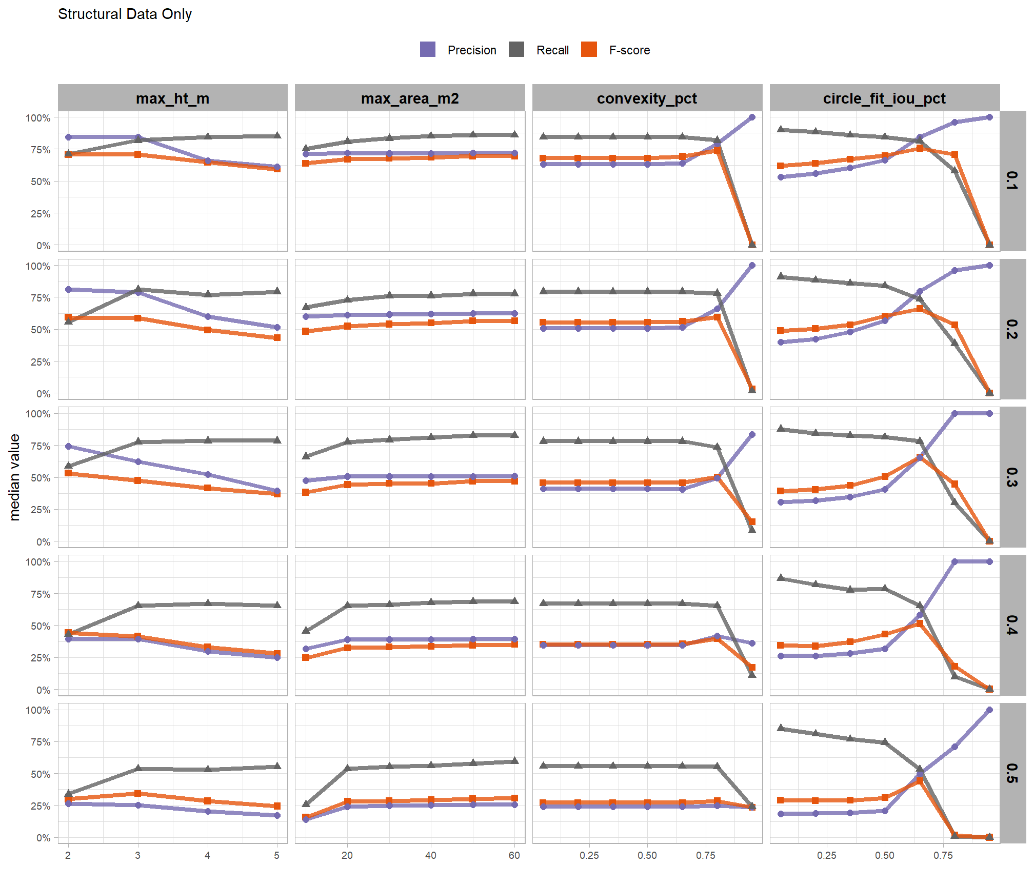
generally, the tends do not appear to vary substantially by CHM resolution but we can see that detection accuracy decreases as CHM resolution becomes more coarse
8.5.2 Main Effects: form quantification
let’s check out the the ability of the method to properly extract the form of the piles by looking at the quantification accuracy metrics where:
- Mean Error (ME) represents the direction of bias (over or under-prediction) in the original units
- RMSE represents the typical magnitude of error in the original units, with a stronger penalty for large errors
- MAPE represents the typical magnitude of error as a percentage, allowing for scale-independent comparisons
as a reminder regarding the form quantification accuracy evaluation, we will assess the method’s accuracy by comparing the true-positive matches using the following metrics:
- Diameter compares the predicted diameter (from the maximum internal distance) to the ground truth field-measured diameter
- Area compares the predicted area from the irregular shape to the image-annotated area based on the potentially irregular pile perimeter
- Height compares the predicted maximum height from the CHM to the ground truth field-measured height
what is the quantification accuracy across all parameter combinations tested for each CHM resolution?
# let's average across all other factors to look at the main effect by parameter for the **MAPE** metrics quantifying the pile form accuracy
# this is a lot of work, so we're going to make it a function
plt_form_quantification_trend <- function(
  df
  , my_subtitle = ""
  , quant_metric = "mape" # rmse, mean, mape
) {
  quant_metric <- dplyr::case_when(
      tolower(quant_metric) == "mape" ~ "mape"
      , tolower(quant_metric) == "rmse" ~ "rmse"
      , tolower(quant_metric) == "mean" ~ "mean"
      , T ~ "mape"
    )

  p <- df %>%
  tidyr::pivot_longer(
    cols = tidyselect::ends_with(paste0("_",quant_metric))
    , names_to = "metric"
    , values_to = "value"
  ) %>%
  tidyr::pivot_longer(
    cols = c(max_ht_m,max_area_m2,convexity_pct,circle_fit_iou_pct,chm_res_m)
    , names_to = "param"
    , values_to = "param_value"
  ) %>%
  dplyr::group_by(param, param_value, metric) %>%
  dplyr::summarise(
    median = median(value,na.rm=T)
    , q25 = stats::quantile(value,na.rm=T,probs = 0.25)
    , q75 = stats::quantile(value,na.rm=T,probs = 0.75)
  ) %>%
  dplyr::ungroup() %>%
  dplyr::mutate(
    param = dplyr::case_when(
        param == "chm_res_m" ~ 1
        , param == "max_ht_m" ~ 2
        , param == "min_area_m2" ~ 3
        , param == "max_area_m2" ~ 4
        , param == "convexity_pct" ~ 5
        , param == "circle_fit_iou_pct" ~ 6
      ) %>%
      factor(
        ordered = T
        , levels = 1:6
        , labels = c(
          "CHM resolution (m)"
          , "max_ht_m"
          , "min_area_m2"
          , "max_area_m2"
          , "convexity_pct"
          , "circle_fit_iou_pct"
        )
      )
    , pile_metric = metric %>%
      stringr::str_remove("(_rmse|_rrmse|_mean|_mape)$") %>%
      stringr::str_extract("(paraboloid_volume|volume|area|height|diameter)") %>%
      factor(
        ordered = T
        , levels = c(
          "volume"
          , "paraboloid_volume"
          , "area"
          , "height"
          , "diameter"
        )
        , labels = c(
          "Volume"
          , "Volume paraboloid"
          , "Area (m2)"
          , "Height (m)"
          , "Diameter (m)"
        )
      )
  ) %>%
  ggplot2::ggplot(
    mapping = ggplot2::aes(y = median, x = param_value, color = pile_metric, fill = pile_metric, group = pile_metric) #, shape = pile_metric)
  ) +
  # ggplot2::geom_ribbon(
  #   mapping = ggplot2::aes(ymin = q25, ymax = q75)
  #   , alpha = 0.2, color = NA
  # ) +
  ggplot2::geom_line(lwd = 1.5, alpha = 0.8) +
  ggplot2::geom_point(size = 2) +
  ggplot2::facet_grid(cols = dplyr::vars(param), rows = dplyr::vars(pile_metric), scales = "free", axes = "all") +
  # ggplot2::scale_color_viridis_d(begin = 0.2, end = 0.8) +
  harrypotter::scale_fill_hp_d(option = "hermionegranger") +
  harrypotter::scale_color_hp_d(option = "hermionegranger") +
  ggplot2::labs(
    x = ""
    , y = paste0(ifelse(quant_metric=="mean","Mean Error", toupper(quant_metric)), " (median)")
    , color = "", fill = ""
    , title = ifelse(quant_metric=="mean","Mean Error", toupper(quant_metric))
  ) +
  ggplot2::theme_light() +
  ggplot2::theme(
    legend.position = "none"
    , strip.text = ggplot2::element_text(size = 11, color = "black", face = "bold")
    , axis.text.x = ggplot2::element_text(size = 7)
    , axis.text.y = ggplot2::element_text(size = 8)
  ) +
  ggplot2::guides(
    color = ggplot2::guide_legend(override.aes = list(shape = 15, linetype = 0, size = 5, alpha = 1))
    , shape = "none"
  )

  if(quant_metric == "mape"){
    p <- p +
      ggplot2::scale_y_continuous(labels = scales::percent, breaks = scales::breaks_extended(10))
  }else{
    p <- p +
      ggplot2::scale_y_continuous(labels = scales::comma, breaks = scales::breaks_extended(10))
  }
  return(p)
}
# plt_form_quantification_trend(param_combos_gt_agg, quant_metric = "mean")
# plt_form_quantification_trend(param_combos_gt_agg, quant_metric = "mape")

# this is a lot of work, so we're going to make it a function
plt_form_quantification_dist2 <- function(
  df
  , my_subtitle = ""
  , show_rug = T
  , quant_metric = "mape" # rmse, mean, mape
) {
  # reshape data to go long by evaluation metric
  df_temp <-
    df %>%
    dplyr::ungroup() %>%
    dplyr::select(
      max_ht_m,max_area_m2,convexity_pct,circle_fit_iou_pct,chm_res_m_desc,chm_res_m
      # quantification
      , tidyselect::ends_with("_rmse")
      , tidyselect::ends_with("_rrmse")
      , tidyselect::ends_with("_mean")
      , tidyselect::ends_with("_mape")
    ) %>%
    tidyr::pivot_longer(
      cols = c(
        tidyselect::ends_with("_rmse")
        , tidyselect::ends_with("_rrmse")
        , tidyselect::ends_with("_mean")
        , tidyselect::ends_with("_mape")
      )
      , names_to = "metric"
      , values_to = "value"
    ) %>%
    dplyr::mutate(
      eval_metric = stringr::str_extract(metric, "(_rmse|_rrmse|_mean|_mape)$") %>%
        stringr::str_remove_all("_") %>%
        stringr::str_replace_all("mean","me") %>%
        toupper() %>%
        factor(
          ordered = T
          , levels = c("ME","RMSE","RRMSE","MAPE")
        )
      , pile_metric = metric %>%
        stringr::str_remove("(_rmse|_rrmse|_mean|_mape)$") %>%
        stringr::str_extract("(paraboloid_volume|volume|area|height|diameter)") %>%
        factor(
          ordered = T
          , levels = c(
            "volume"
            , "paraboloid_volume"
            , "area"
            , "height"
            , "diameter"
          )
          , labels = c(
            "Volume"
            , "Volume paraboloid"
            , "Area (m2)"
            , "Height (m)"
            , "Diameter (m)"
          )
        )
    )

  # plot
  # chm check
  nrow_check <- df %>%
    dplyr::count(chm_res_m_desc) %>%
    dplyr::pull(n) %>%
    max()

  # plot
  if(nrow_check<=15){
    # round
    df_temp <- df_temp %>%
      dplyr::filter(
        eval_metric==dplyr::case_when(
          tolower(quant_metric) == "mape" ~ "MAPE"
          , tolower(quant_metric) == "rmse" ~ "RMSE"
          , tolower(quant_metric) == "mean" ~ "ME"
          , T ~ "MAPE"
        )
      ) %>%
      dplyr::mutate(
        value = dplyr::case_when(
          eval_metric %in% c("RRMSE", "MAPE") ~ round(value,2)
          , T ~ round(value,1)
        )
      )
    # agg for median plotting
    xxxdf_temp <- df_temp %>%
      dplyr::group_by(chm_res_m_desc,pile_metric,eval_metric) %>%
      dplyr::summarise(value = median(value,na.rm=T)) %>%
      dplyr::ungroup() %>%
      dplyr::mutate(
        value_lab = paste0(
            "median:\n"
          , dplyr::case_when(
            eval_metric %in% c("RRMSE", "MAPE") ~ scales::percent(value,accuracy=1)
            , eval_metric == "ME" ~ scales::comma(value,accuracy=0.1)
            , T ~ scales::comma(value,accuracy=0.1)
          )
        )
      )

    # plot
    p <-
      df_temp %>%
      dplyr::count(chm_res_m_desc,pile_metric,value) %>%
        ggplot2::ggplot(mapping = ggplot2::aes(x=value,color = pile_metric,fill = pile_metric)) +
        ggplot2::geom_vline(
          data = xxxdf_temp %>%
            dplyr::filter(
              eval_metric==dplyr::case_when(
                tolower(quant_metric) == "mape" ~ "MAPE"
                , tolower(quant_metric) == "rmse" ~ "RMSE"
                , tolower(quant_metric) == "mean" ~ "ME"
                , T ~ "MAPE"
              )
            )
          , mapping = ggplot2::aes(xintercept = value)
          , color = "gray44", linetype = "dashed"
        ) +
        ggplot2::geom_segment(
          mapping = ggplot2::aes(y=n,yend=0)
          , lwd = 2, alpha = 0.8
        ) +
        ggplot2::geom_point(
          mapping = ggplot2::aes(y=n)
          , alpha = 1
          , shape = 21, color = "gray44", size = 5
        ) +
        ggplot2::geom_text(
          mapping = ggplot2::aes(y=n,label=n)
          , size = 2.5, color = "white"
          # , vjust = -0.01
        ) +
        ggplot2::scale_y_continuous(expand = ggplot2::expansion(mult = c(0, .2))) +
        harrypotter::scale_fill_hp_d(option = "hermionegranger") +
        harrypotter::scale_color_hp_d(option = "hermionegranger") +
        ggplot2::geom_text(
          data = xxxdf_temp %>%
            dplyr::filter(
              eval_metric==dplyr::case_when(
                tolower(quant_metric) == "mape" ~ "MAPE"
                , tolower(quant_metric) == "rmse" ~ "RMSE"
                , tolower(quant_metric) == "mean" ~ "ME"
                , T ~ "MAPE"
              )
            )
          , mapping = ggplot2::aes(
            x = -Inf, y = Inf # always in upper left?
            # x = value, y = 0
            , label = value_lab
          )
          , hjust = -0.1, vjust = 1 # always in upper left?
          # , hjust = -0.1, vjust = -5
          , size = 2.5
          , color = "black"
        ) +
        ggplot2::facet_grid(cols = dplyr::vars(pile_metric), rows = dplyr::vars(chm_res_m_desc), scales = "free") +
        ggplot2::labs(
          x = "", y = ""
          , subtitle = my_subtitle
          , title = dplyr::case_when(
            tolower(quant_metric) == "mape" ~ "MAPE"
            , tolower(quant_metric) == "rmse" ~ "RMSE"
            , tolower(quant_metric) == "mean" ~ "Mean Error"
            , T ~ "MAPE"
          )
        ) +
        ggplot2::theme_light() +
        ggplot2::theme(
          legend.position = "none"
          , strip.text.x = ggplot2::element_text(size = 11, color = "black", face = "bold")
          , strip.text.y = ggplot2::element_text(size = 9, color = "black", face = "bold")
          , axis.text.x = ggplot2::element_text(size = 7)
          , axis.text.y = ggplot2::element_blank()
          , axis.ticks.y = ggplot2::element_blank()
          , panel.grid.major.y = ggplot2::element_blank()
          , panel.grid.minor.y = ggplot2::element_blank()
          , plot.subtitle = ggplot2::element_text(size = 8)
        )

  }else{
    # aggregate
    xxxdf_temp <- df_temp %>%
      dplyr::group_by(chm_res_m_desc,pile_metric,eval_metric) %>%
      dplyr::summarise(value = median(value,na.rm=T)) %>%
      dplyr::ungroup() %>%
      dplyr::mutate(
        value_lab = paste0(
            "median:\n"
          , dplyr::case_when(
            eval_metric %in% c("RRMSE", "MAPE") ~ scales::percent(value,accuracy=0.1)
            , eval_metric == "ME" ~ scales::comma(value,accuracy=0.01)
            , T ~ scales::comma(value,accuracy=0.1)
          )
        )
      )

    p <-
      df_temp %>%
      dplyr::filter(
        eval_metric==dplyr::case_when(
          tolower(quant_metric) == "mape" ~ "MAPE"
          , tolower(quant_metric) == "rmse" ~ "RMSE"
          , tolower(quant_metric) == "mean" ~ "ME"
          , T ~ "MAPE"
        )
      ) %>%
          ggplot2::ggplot() +
          # ggplot2::geom_vline(xintercept = 0, color = "gray") +
          ggplot2::geom_density(mapping = ggplot2::aes(x = value, y = ggplot2::after_stat(scaled), fill = pile_metric), color = NA, alpha = 0.9) +
          harrypotter::scale_fill_hp_d(option = "hermionegranger") +
          harrypotter::scale_color_hp_d(option = "hermionegranger") +
          ggplot2::geom_vline(
            data = xxxdf_temp %>%
              dplyr::filter(
                eval_metric==dplyr::case_when(
                  tolower(quant_metric) == "mape" ~ "MAPE"
                  , tolower(quant_metric) == "rmse" ~ "RMSE"
                  , tolower(quant_metric) == "mean" ~ "ME"
                  , T ~ "MAPE"
                )
              )
            , mapping = ggplot2::aes(xintercept = value)
            , color = "gray44", linetype = "dashed"
          ) +
          ggplot2::geom_text(
            data = xxxdf_temp %>%
              dplyr::filter(
                eval_metric==dplyr::case_when(
                  tolower(quant_metric) == "mape" ~ "MAPE"
                  , tolower(quant_metric) == "rmse" ~ "RMSE"
                  , tolower(quant_metric) == "mean" ~ "ME"
                  , T ~ "MAPE"
                )
              )
            , mapping = ggplot2::aes(
              x = -Inf, y = Inf # always in upper left?
              # x = value, y = 0
              , label = value_lab
            )
            , hjust = -0.1, vjust = 1 # always in upper left?
            # , hjust = -0.1, vjust = -5
            , size = 2.5
          ) +
          ggplot2::facet_grid(cols = dplyr::vars(pile_metric), rows = dplyr::vars(chm_res_m_desc), scales = "free") +
          ggplot2::labs(
            x = "", y = ""
            , subtitle = my_subtitle
            , title = dplyr::case_when(
              tolower(quant_metric) == "mape" ~ "MAPE"
              , tolower(quant_metric) == "rmse" ~ "RMSE"
              , tolower(quant_metric) == "mean" ~ "Mean Error"
              , T ~ "MAPE"
            )
          ) +
          ggplot2::theme_light() +
          ggplot2::theme(
            legend.position = "none"
            , strip.text.x = ggplot2::element_text(size = 11, color = "black", face = "bold")
            , strip.text.y = ggplot2::element_text(size = 9, color = "black", face = "bold")
            , axis.text.x = ggplot2::element_text(size = 7)
            , axis.text.y = ggplot2::element_blank()
            , axis.ticks.y = ggplot2::element_blank()
            , panel.grid.major.y = ggplot2::element_blank()
            , panel.grid.minor.y = ggplot2::element_blank()
            , plot.subtitle = ggplot2::element_text(size = 8)
          )

        if(show_rug){
          p <- p + ggplot2::geom_rug(mapping = ggplot2::aes(x = value, color = pile_metric))
        }
  }

  if(
    dplyr::case_when(
      tolower(quant_metric) == "mape" ~ "MAPE"
      , tolower(quant_metric) == "rmse" ~ "RMSE"
      , tolower(quant_metric) == "mean" ~ "ME"
      , T ~ "MAPE"
    ) %in% c("RRMSE", "MAPE")
  ){
    return(p+ggplot2::scale_x_continuous(labels = scales::percent_format(accuracy = 1)))
  }else{
    return(p)
  }

}
8.5.2.1 MAPE
MAPE represents the typical magnitude of error as a percentage, allowing for scale-independent comparisons
distribution across all parameter combinations tested
# plot it
plt_form_quantification_dist2(
  df = param_combos_gt_agg
  , quant_metric = "mape"
  , paste0(
     "Structural Data Only"
      , "\ndistribution of pile form quantification accuracy metrics for all"
     , " (n="
     , scales::comma(n_combos_tested_chm, accuracy = 1)
     , ") "
     , "parameter combinations tested"
  )
  , show_rug = F
)
let’s average across all other factors to look at the median main effect by parameter and quantification metric

Across the different pile measurement metrics, there are non-linear trends between MAPE and CHM resolution, convexity_pct, and circle_fit_iou_pct. Additionally, the height MAPE does not appear to vary much across the different CHM resolutions tested, so non-linear trends between the height measurement error and parameter settings may be less consequential.
8.5.2.2 Mean Error (ME)
Mean Error (ME) represents the direction of bias (over or under-prediction) in the original units
distribution across all parameter combinations tested
# plot it
plt_form_quantification_dist2(
  df = param_combos_gt_agg
  , quant_metric = "mean"
  , paste0(
     "Structural Data Only"
      , "\ndistribution of pile form quantification accuracy metrics for all"
     , " (n="
     , scales::comma(n_combos_tested_chm, accuracy = 1)
     , ") "
     , "parameter combinations tested"
  )
  , show_rug = F
)
let’s average across all other factors to look at the median main effect by parameter and quantification metric
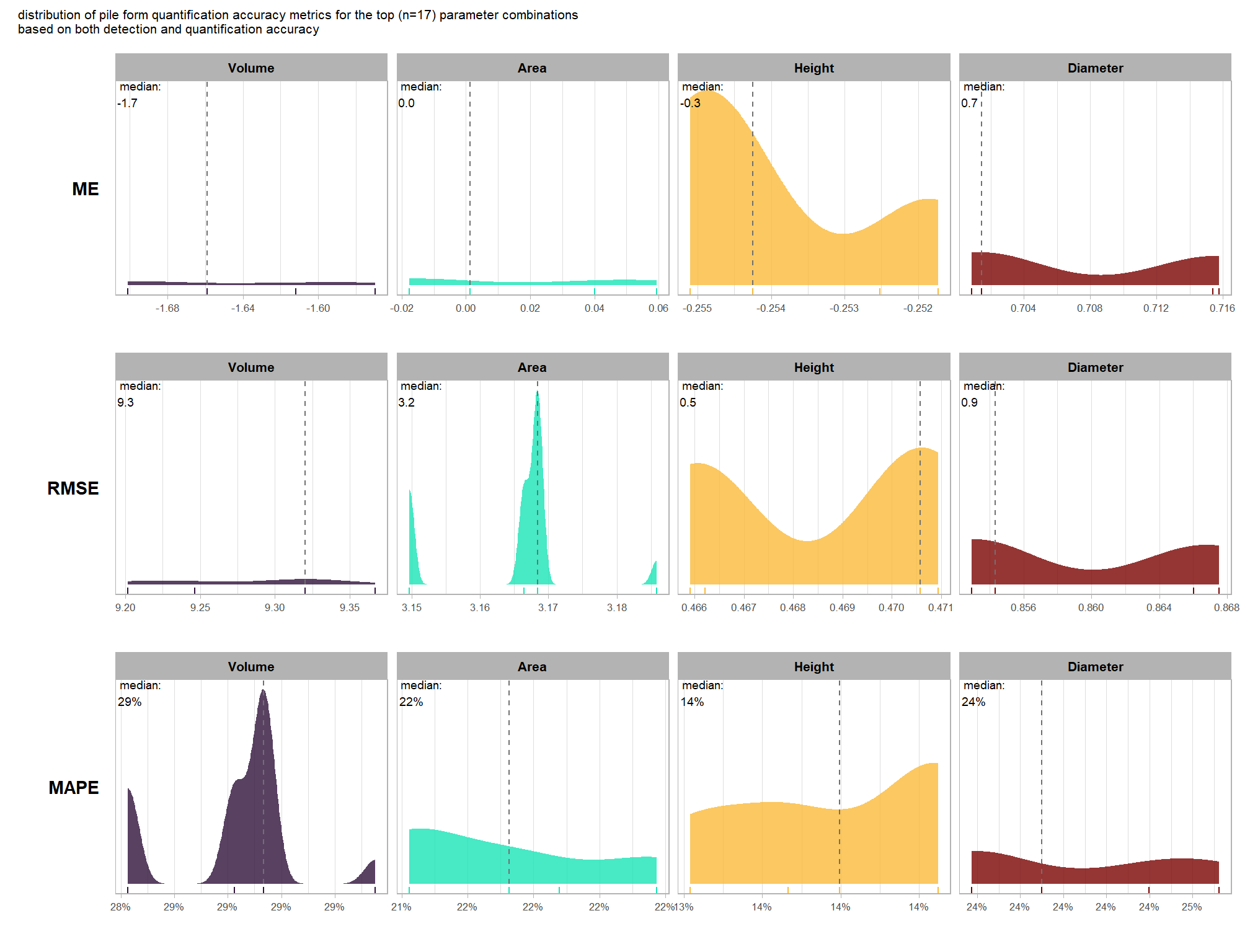
8.5.2.3 RMSE
RMSE represents the typical magnitude of error in the original units, with a stronger penalty for large errors
# plot it
plt_form_quantification_dist2(
  df = param_combos_gt_agg
  , quant_metric = "rmse"
  , paste0(
     "Structural Data Only"
      , "\ndistribution of pile form quantification accuracy metrics for all"
     , " (n="
     , scales::comma(n_combos_tested_chm, accuracy = 1)
     , ") "
     , "parameter combinations tested"
  )
  , show_rug = F
)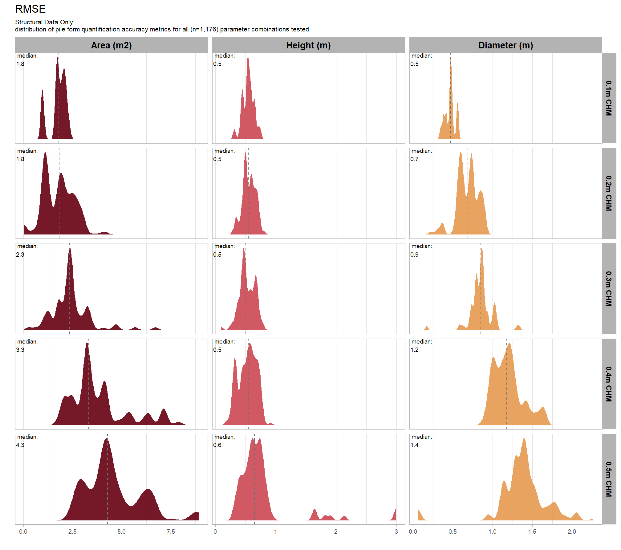
let’s average across all other factors to look at the median main effect by parameter and quantification metric
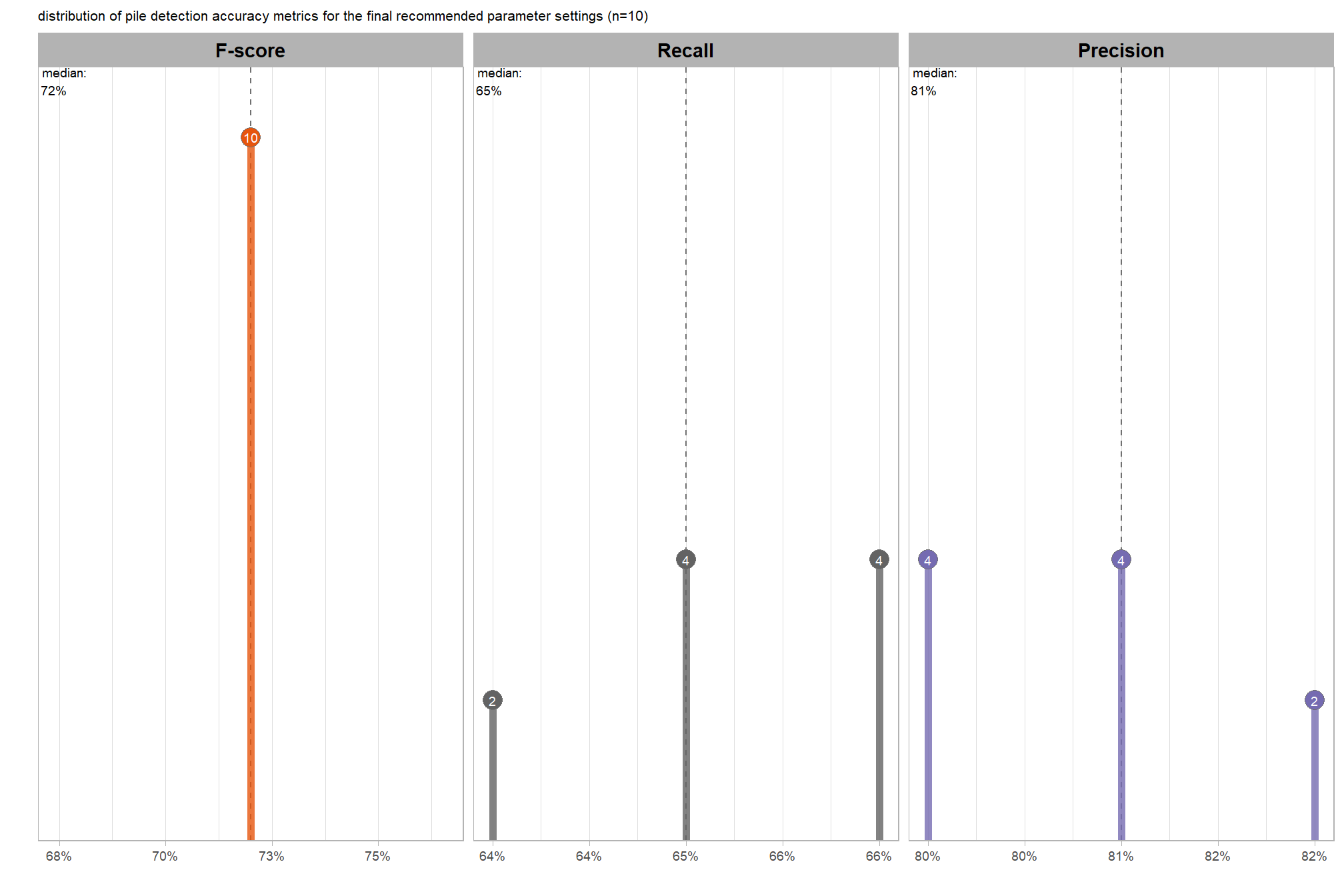
8.5.3 Best settings
Of the parameter levels we tested to generate these accuracy point estimates, let’s identify the best-performing parameter combinations that not only balance detection and quantification accuracy but also achieve the highest recall rates. we’ll select these by choosing any combination whose recall rate is at least one standard deviation above the average for this top group. if no combinations meet this criterion, we will instead select the top 10 combinations based on their recall rates.
8.5.3.1 Overall (across CHM resolution)
To select the best-performing parameter combinations, we will prioritize those that balance detection and quantification accuracy. From this group, we will then identify the settings that achieve the highest pile detection rates (recall). We emphasize that these recommendations are for users who can generate a CHM from the original point cloud. This is critical because creating a new CHM at the desired resolution is a fundamentally different process than simply disaggregating an existing, coarser raster.
we’ll use the F-Score and the average rank of the MAPE metrics across all form measurements (i.e. height, diameter, area, volume) to determine the best overall list
##################### START USER DEFINED #####################
# what percent should we classify as top?
pct_th_top <- 0.01
# of those top, how many should be selected by recall?
n_th_top <- 12
##################### END USER DEFINED #####################
# math on user defined to label stuff
# structural only
n_combos_top_overall <- n_combos_tested*pct_th_top
n_th_top_chm <- round(n_th_top/2)
pct_th_top_chm <- pct_th_top*2
n_combos_top_chm <- floor(n_combos_tested_chm*pct_th_top_chm) # double it so we look at more than 14??
n_combos_top_spectral_chm <- floor(n_combos_tested_spectral_chm*pct_th_top_chm)
# param_combos_gt_agg %>% nrow()
# param_combos_gt_agg %>% dplyr::select(tidyselect::ends_with("_mape")) %>% dplyr::glimpse()
param_combos_ranked <-
param_combos_gt_agg %>%
##########
# first. find overall top combinations irrespective of CHM res
##########
dplyr::ungroup() %>%
dplyr::mutate(
# label combining params
lab = stringr::str_c(max_ht_m,max_area_m2,convexity_pct,circle_fit_iou_pct,chm_res_m, sep = ":")
, dplyr::across(
.cols = c(tidyselect::ends_with("_mape"))
, .fn = ~dplyr::percent_rank(-.x)
, .names = "ovrall_pct_rank_quant_{.col}"
)
, dplyr::across(
.cols = c(f_score)
# .cols = c(f_score,recall)
, .fn = ~dplyr::percent_rank(.x)
, .names = "ovrall_pct_rank_det_{.col}"
)
) %>%
##########
# second. find top combinations by CHM res
##########
dplyr::group_by(chm_res_m) %>%
dplyr::mutate(
dplyr::across(
.cols = c(tidyselect::ends_with("_mape") & !tidyselect::starts_with("ovrall_pct_rank_"))
, .fn = ~dplyr::percent_rank(-.x)
, .names = "chm_pct_rank_quant_{.col}"
)
, dplyr::across(
.cols = c(f_score)
# .cols = c(f_score,recall)
, .fn = ~dplyr::percent_rank(.x)
, .names = "chm_pct_rank_det_{.col}"
)
) %>%
# now get the max of these pct ranks by row
dplyr::rowwise() %>%
dplyr::mutate(
ovrall_pct_rank_quant_mean = mean(
dplyr::c_across(
tidyselect::starts_with("ovrall_pct_rank_quant_")
)
, na.rm = T
)
, ovrall_pct_rank_det_mean = mean(
dplyr::c_across(
tidyselect::starts_with("ovrall_pct_rank_det_")
)
, na.rm = T
)
, chm_pct_rank_quant_mean = mean(
dplyr::c_across(
tidyselect::starts_with("chm_pct_rank_quant_")
)
, na.rm = T
)
, chm_pct_rank_det_mean = mean(
dplyr::c_across(
tidyselect::starts_with("chm_pct_rank_det_")
)
, na.rm = T
)
) %>%
dplyr::ungroup() %>%
# fill na values
dplyr::mutate(
dplyr::across(
.cols = c(ovrall_pct_rank_det_mean, ovrall_pct_rank_quant_mean, chm_pct_rank_det_mean, chm_pct_rank_quant_mean)
, .fn = ~ifelse(is.na(.x),0,.x)
)
) %>%
# now make quadrant var
dplyr::mutate(
# groupings for the quadrant plot
ovrall_accuracy_grp = dplyr::case_when(
ovrall_pct_rank_det_mean>=0.95 & ovrall_pct_rank_quant_mean>=0.95 ~ 1
, ovrall_pct_rank_det_mean>=0.90 & ovrall_pct_rank_quant_mean>=0.90 ~ 2
, ovrall_pct_rank_det_mean>=0.75 & ovrall_pct_rank_quant_mean>=0.75 ~ 3
, ovrall_pct_rank_det_mean>=0.50 & ovrall_pct_rank_quant_mean>=0.50 ~ 4
, ovrall_pct_rank_det_mean>=0.50 & ovrall_pct_rank_quant_mean<0.50 ~ 5
, ovrall_pct_rank_det_mean<0.50 & ovrall_pct_rank_quant_mean>=0.50 ~ 6
, T ~ 7
) %>%
factor(
ordered = T
, levels = 1:7
, labels = c(
"top 5% detection & quantification" # ovrall_pct_rank_mean>=0.95 & ovrall_pct_rank_f_score>=0.95 ~ 1
, "top 10% detection & quantification" # ovrall_pct_rank_mean>=0.90 & ovrall_pct_rank_f_score>=0.90 ~ 2
, "top 25% detection & quantification" # ovrall_pct_rank_mean>=0.75 & ovrall_pct_rank_f_score>=0.75 ~ 3
, "top 50% detection & quantification" # ovrall_pct_rank_mean>=0.50 & ovrall_pct_rank_f_score>=0.50 ~ 4
, "top 50% quantification" # ovrall_pct_rank_mean>=0.50 & ovrall_pct_rank_f_score<0.50 ~ 5
, "top 50% detection" # ovrall_pct_rank_mean<0.50 & ovrall_pct_rank_f_score>=0.50 ~ 6
, "bottom 50% detection & quantification"
)
)
, chm_accuracy_grp = dplyr::case_when(
chm_pct_rank_det_mean>=0.95 & chm_pct_rank_quant_mean>=0.95 ~ 1
, chm_pct_rank_det_mean>=0.90 & chm_pct_rank_quant_mean>=0.90 ~ 2
, chm_pct_rank_det_mean>=0.75 & chm_pct_rank_quant_mean>=0.75 ~ 3
, chm_pct_rank_det_mean>=0.50 & chm_pct_rank_quant_mean>=0.50 ~ 4
, chm_pct_rank_det_mean>=0.50 & chm_pct_rank_quant_mean<0.50 ~ 5
, chm_pct_rank_det_mean<0.50 & chm_pct_rank_quant_mean>=0.50 ~ 6
, T ~ 7
) %>%
factor(
ordered = T
, levels = 1:7
, labels = c(
"top 5% detection & quantification" # chm_pct_rank_mean>=0.95 & chm_pct_rank_f_score>=0.95 ~ 1
, "top 10% detection & quantification" # chm_pct_rank_mean>=0.90 & chm_pct_rank_f_score>=0.90 ~ 2
, "top 25% detection & quantification" # chm_pct_rank_mean>=0.75 & chm_pct_rank_f_score>=0.75 ~ 3
, "top 50% detection & quantification" # chm_pct_rank_mean>=0.50 & chm_pct_rank_f_score>=0.50 ~ 4
, "top 50% quantification" # chm_pct_rank_mean>=0.50 & chm_pct_rank_f_score<0.50 ~ 5
, "top 50% detection" # chm_pct_rank_mean<0.50 & chm_pct_rank_f_score>=0.50 ~ 6
, "bottom 50% detection & quantification"
)
)
,
) %>%
##########
# first. find overall top combinations irrespective of CHM res
##########
dplyr::ungroup() %>%
dplyr::mutate(
ovrall_balanced_pct_rank = dplyr::percent_rank( (ovrall_pct_rank_det_mean+ovrall_pct_rank_quant_mean)/2 ) # equally weight quant and detection
, ovrall_lab = forcats::fct_reorder(lab, ovrall_balanced_pct_rank)
) %>%
dplyr::arrange(desc(ovrall_balanced_pct_rank),desc(ovrall_pct_rank_det_mean),desc(ovrall_pct_rank_quant_mean)) %>%
dplyr::mutate(
ovrall_balanced_rank = dplyr::row_number()
# is_top_overall = using rows in case not all combos resulted in piles and/or
# there are many ties in the data leading to no records with a percent rank <= pct_th_top (e.g. many tied at 98%)
, is_top_overall = dplyr::row_number()<=(n_combos_top_overall)
# ovrall_balanced_pct_rank>=(1-pct_th_top)
) %>%
dplyr::arrange(desc(is_top_overall),desc(recall),desc(ovrall_pct_rank_det_mean),desc(ovrall_pct_rank_quant_mean),ovrall_balanced_rank) %>%
dplyr::mutate(is_final_selection = is_top_overall & dplyr::row_number()<=n_th_top) %>%
##########
# second. find top combinations by CHM res
##########
dplyr::group_by(chm_res_m) %>%
dplyr::mutate(
chm_balanced_pct_rank = dplyr::percent_rank( (chm_pct_rank_det_mean+chm_pct_rank_quant_mean)/2 ) # equally weight quant and detection
, chm_lab = forcats::fct_reorder(lab, chm_balanced_pct_rank)
) %>%
dplyr::arrange(chm_res_m,desc(chm_balanced_pct_rank),desc(chm_pct_rank_det_mean),desc(chm_pct_rank_quant_mean),ovrall_balanced_rank) %>%
dplyr::mutate(
chm_balanced_rank = dplyr::row_number()
# is_top_chm = using rows in case not all combos resulted in piles and/or
# there are many ties in the data leading to no records with a percent rank <= pct_th_top (e.g. many tied at 98%)
, is_top_chm = dplyr::row_number()<=n_combos_top_chm # double it so we look at more than 14??
# chm_balanced_pct_rank>=(1-pct_th_top)
) %>%
dplyr::arrange(chm_res_m,desc(is_top_chm),desc(recall),desc(chm_pct_rank_det_mean),desc(chm_pct_rank_quant_mean),ovrall_balanced_rank) %>%
dplyr::mutate(is_final_selection_chm = is_top_chm & dplyr::row_number()<=n_th_top_chm) %>% # half it because it's going to be a lot to show in our facet ggplot
##### clean up
dplyr::ungroup() %>%
dplyr::select(-c(
c(tidyselect::ends_with("_mape") & tidyselect::starts_with("ovrall_pct_rank_"))
, c(tidyselect::ends_with("_mape") & tidyselect::starts_with("chm_pct_rank_"))
, c(tidyselect::ends_with("_f_score") & tidyselect::starts_with("ovrall_pct_rank_"))
, c(tidyselect::ends_with("_f_score") & tidyselect::starts_with("chm_pct_rank_"))
))
# huh?
# param_combos_ranked %>% dplyr::glimpse()
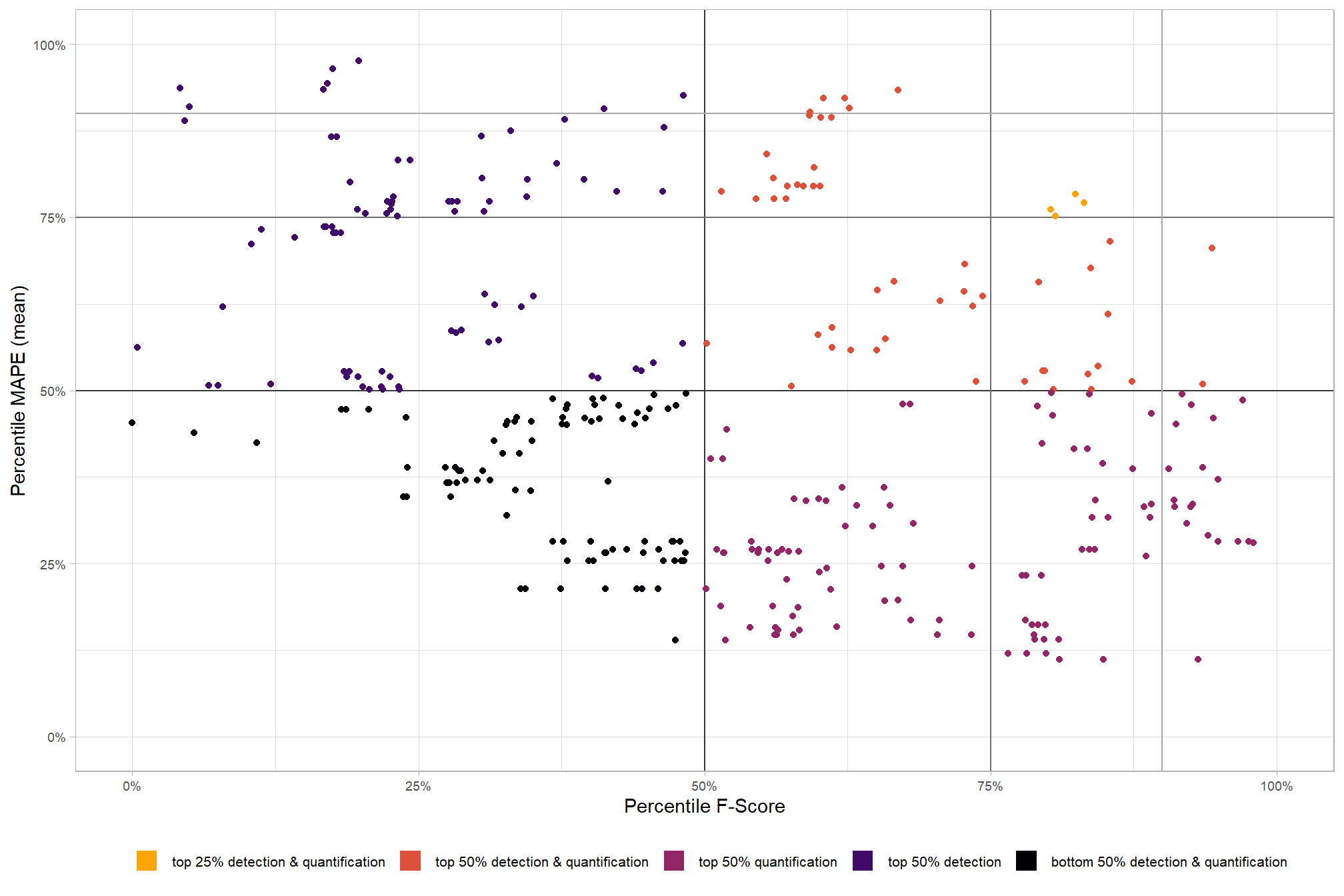
# param_combos_ranked %>% dplyr::count(is_final_selection)to determine the combinations that achieved the best balance between both detection and quantification accuracy, we’re selecting the parameter combinations that are in the upper-right of the quadrant plot. That is, the parameter combinations that performed best at both pile detection accuracy and pile form quantification accuracy
# plot
param_combos_ranked %>%
  ggplot2::ggplot(
    mapping=ggplot2::aes(x = ovrall_pct_rank_det_mean, y = ovrall_pct_rank_quant_mean, color = ovrall_accuracy_grp)
  ) +
  ggplot2::geom_vline(xintercept = 0.5, color = "gray22") +
  ggplot2::geom_hline(yintercept = 0.5, color = "gray22") +
  ggplot2::geom_vline(xintercept = 0.75, color = "gray44") +
  ggplot2::geom_hline(yintercept = 0.75, color = "gray44") +
  ggplot2::geom_vline(xintercept = 0.9, color = "gray66") +
  ggplot2::geom_hline(yintercept = 0.9, color = "gray66") +
  ggplot2::geom_point() +
  ggplot2::scale_colour_viridis_d(direction = -1) +
  ggplot2::scale_x_continuous(
    labels = scales::percent_format(accuracy = 1)
    , limits = c(0,1)
  ) +
  ggplot2::scale_y_continuous(
    labels = scales::percent_format(accuracy = 1)
    , limits = c(0,1)
  ) +
  ggplot2::labs(
    x = "Percentile F-Score", y = "Percentile MAPE (mean)"
    , color = ""
    , subtitle = "Structural Data Only"
  ) +
  ggplot2::theme_light() +
  ggplot2::theme(
    legend.position = "bottom"
    , legend.text = ggplot2::element_text(size = 8)
    , strip.text = ggplot2::element_text(size = 11, color = "black", face = "bold")
    , axis.text = ggplot2::element_text(size = 7)
  ) +
  ggplot2::guides(
    color = ggplot2::guide_legend(override.aes = list(shape = 15, linetype = 0, size = 5, alpha = 1))
    , shape = "none"
  )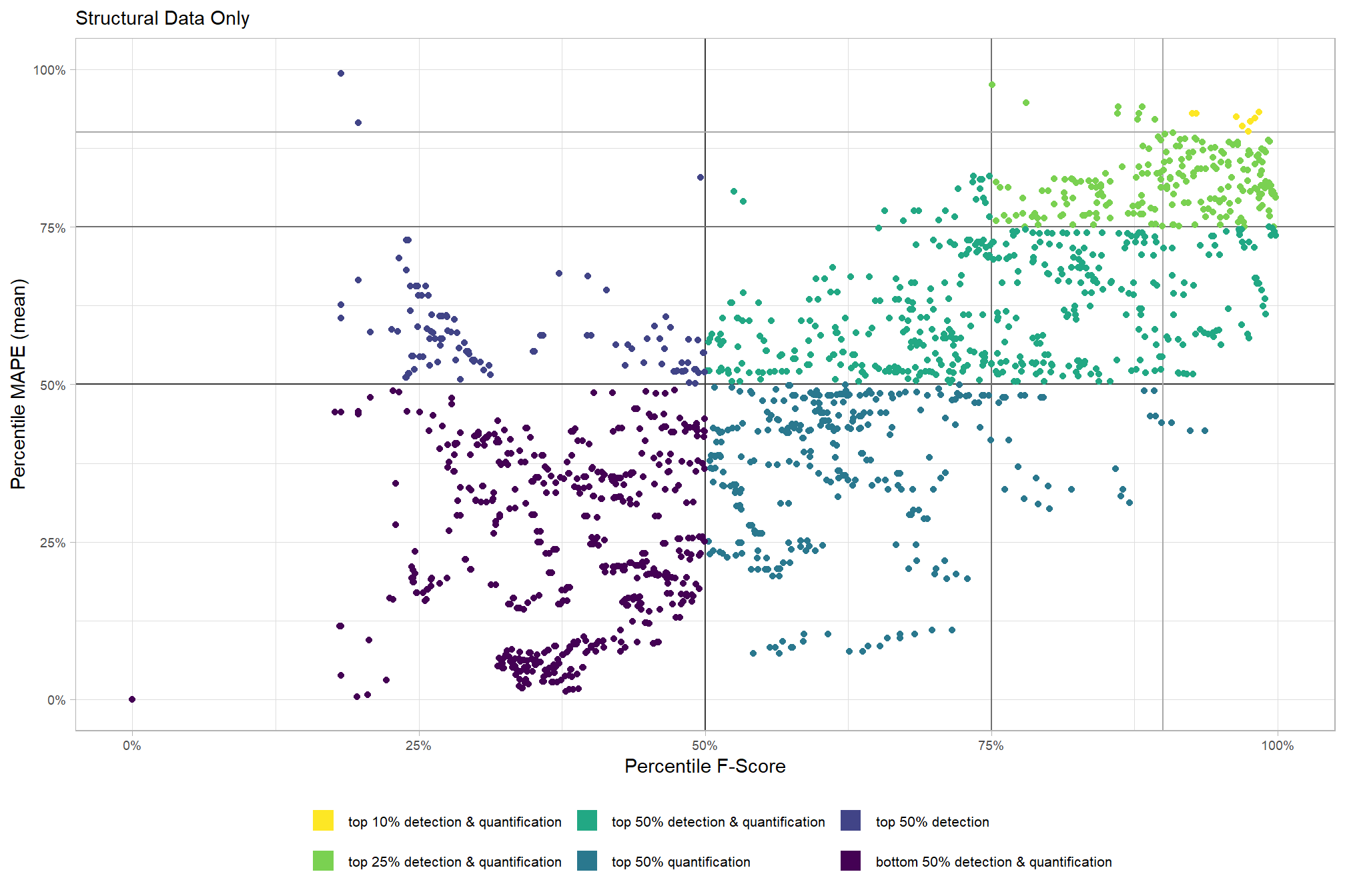
8.5.3.1.1 Top 1.0%
let’s check out the parameter settings of the top 1.0% (n=59) from all 5,880 combinations tested. these are “votes” for the parameter setting based on the combinations that achieved the best balance between both detection and quantification accuracy.
pal_param <- viridis::cividis(n=6, alpha = 0.9)
param_combos_ranked %>%
  dplyr::filter(is_top_overall) %>%
  dplyr::select(tidyselect::contains("f_score"), max_ht_m,max_area_m2,convexity_pct,circle_fit_iou_pct,chm_res_m) %>%
  tidyr::pivot_longer(
    cols = c(max_ht_m,max_area_m2,convexity_pct,circle_fit_iou_pct,chm_res_m)
    , names_to = "metric"
    , values_to = "value"
  ) %>%
  dplyr::count(metric, value) %>%
  dplyr::group_by(metric) %>%
  dplyr::mutate(
    pct=n/sum(n)
    , lab = paste0(scales::percent(pct,accuracy=0.1), "\nn=", scales::comma(n,accuracy=1))
  ) %>%
  ggplot2::ggplot(
    mapping = ggplot2::aes(x = factor(value), y=pct, label=lab, fill = metric)
  ) +
  ggplot2::geom_col(width = 0.6) +
  ggplot2::geom_text(color = "black", size = 2.5, vjust = -0.2) +
  ggplot2::facet_wrap(facets = dplyr::vars(metric), ncol=2, scales = "free_x") +
  ggplot2::scale_y_continuous(
    breaks = seq(0,1,by=0.2)
    , labels = scales::percent
    , expand = ggplot2::expansion(mult = c(0,0.2))
  ) +
  ggplot2::scale_fill_manual(values = pal_param[1:5]) +
  ggplot2::labs(
    x = "parameter setting", y = ""
    , fill = ""
    , subtitle = paste0(
      "Structural Data Only"
       , "\nparameter settings of top "
       , scales::percent(pct_th_top,accuracy=0.1)
       , " (n="
       , scales::comma(n_combos_top_overall, accuracy = 1)
       , ") "
       , "overall parameter combinations tested\nbased on both detection and quantification accuracy"
    )
  ) +
  ggplot2::theme_light() +
  ggplot2::theme(
    legend.position = "none"
    , strip.text = ggplot2::element_text(size = 11, color = "black", face = "bold")
    , axis.text.y = ggplot2::element_text(size = 6)
    , axis.text.x = ggplot2::element_text(size = 8)
    , plot.subtitle = ggplot2::element_text(size = 8)
  )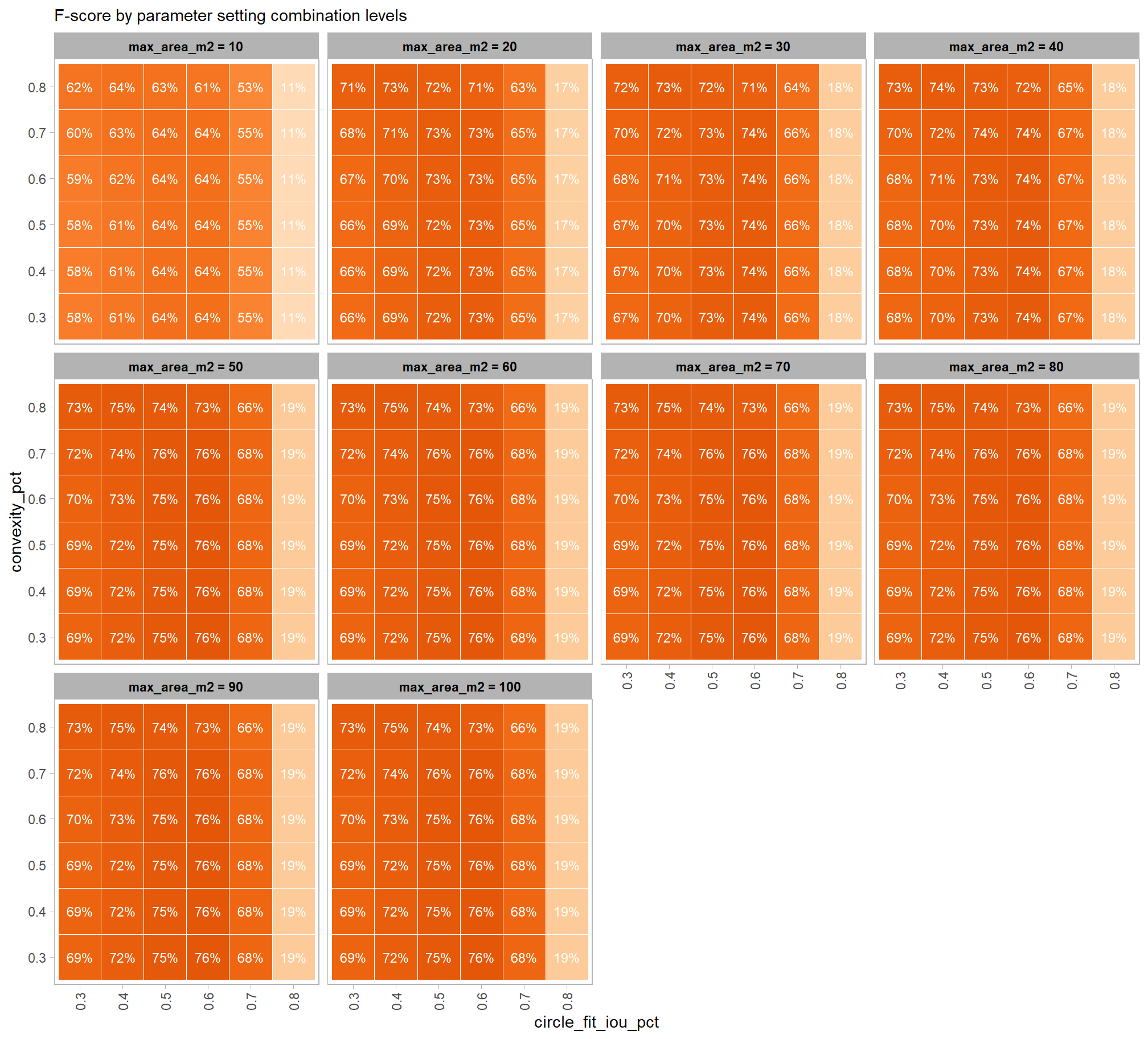
these results indicate that the finer resolution CHM data is preferable for detecting and quantifying slash piles from aerial point cloud data using our methodology. Given our study site, there is a single max_ht_m setting that best fits the data collected at this site. The remaining structural parameters tested (max_area_m2, convexity_pct, circle_fit_iou_pct) can yield good results over a broad setting range but it is important to remember that the influence of these settings is dependent on the value of the other parameters. That is, the effect of one parameter (e.g., convexity_pct) on the accuracy metrics changes depending on the value of another parameter (e.g., circle_fit_iou_pct).
what is the expected detection accuracy of the top 1.0% (n=59) combinations tested?
plt_detection_dist(
  df = param_combos_ranked %>% dplyr::filter(is_top_overall) %>% dplyr::select(!tidyselect::contains("_pct_rank_"))
  , paste0(
    "Structural Data Only"
    , "\ndistribution of pile detection metrics for top "
    , scales::percent(pct_th_top,accuracy=0.1)
    , " (n="
    , scales::comma(n_combos_top_overall, accuracy = 1)
    , ") "
    , "overall parameter combinations tested\nbased on both detection and quantification accuracy"
  )
)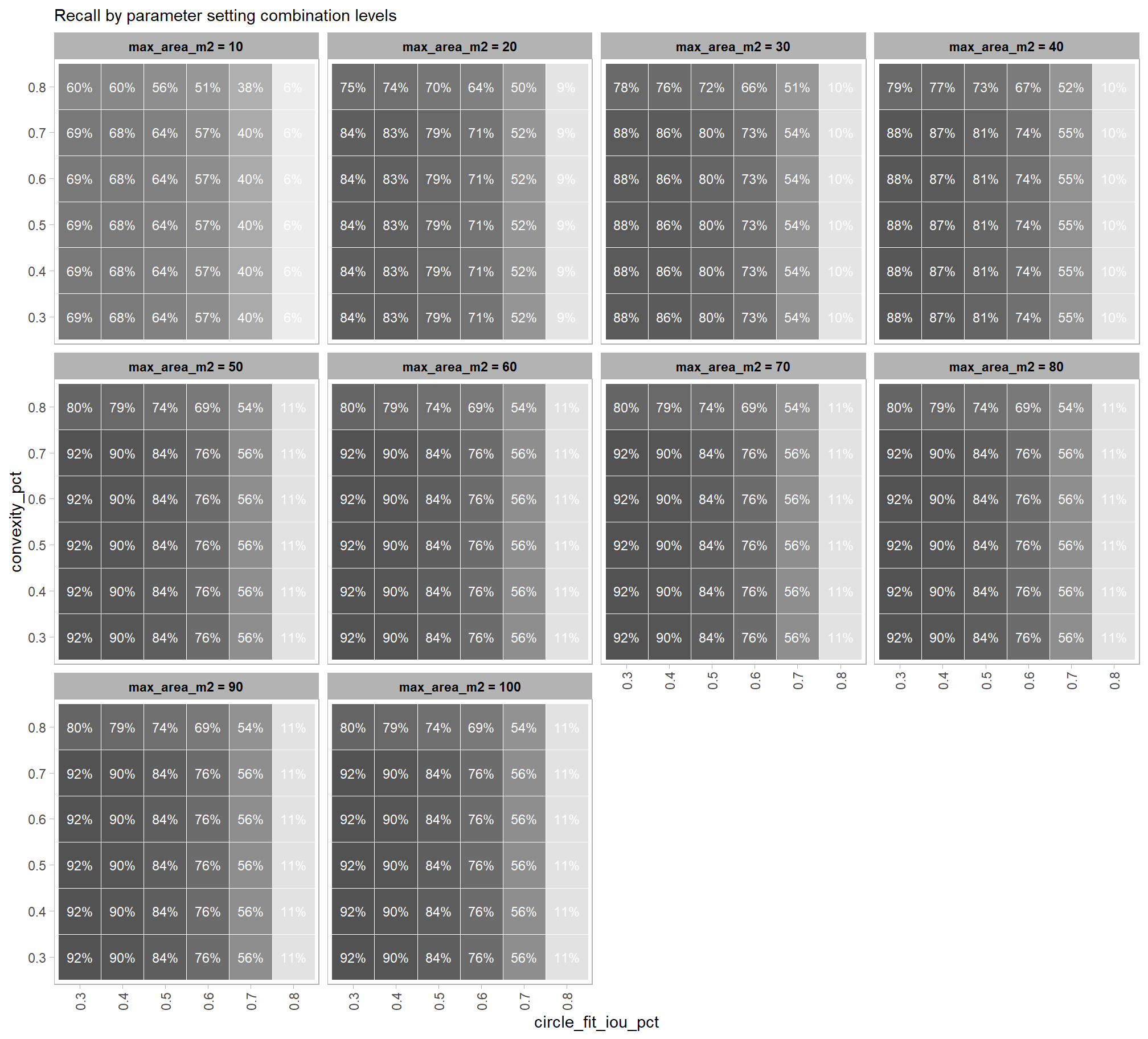
These results are promising for our detection methodology when given structural data only (i.e. CHM data but no spectral data). Using the structural data alone, the best performing parameterization settings of those tested achieved an F-score (balanced detection accuracy) of approximately 77.1% with a detection rate (recall) of approximately 71.1%
what is the expected quantification accuracy of the top 1.0% (n=59) combinations tested?
# plot it
plt_form_quantification_dist(
  df = param_combos_ranked %>% dplyr::filter(is_top_overall) %>% dplyr::select(!tidyselect::contains("_pct_rank_"))
  , paste0(
    "Structural Data Only"
    , "\ndistribution of pile form quantification metrics for the top "
    , scales::percent(pct_th_top,accuracy=0.1)
    , " (n="
    , scales::comma(n_combos_top_overall, accuracy = 1)
    , ") "
    , "overall parameter combinations tested\nbased on both detection and quantification accuracy"
  )
)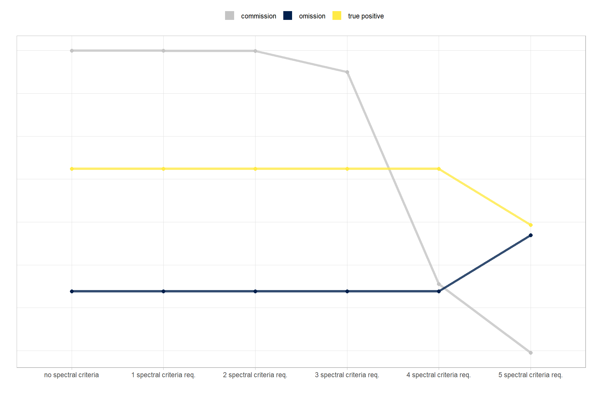
These results are just as promising as the detection accuracy results and indicate that when given structural data only (i.e. CHM data but no spectral data) the methodology can accurately quantify slash pile height and diameter with sub-meter (i.e. < 1m) accuracy when compared with field-measured values. Over the range of parameter settings tested, the methodology also performs well at determining the pile footprint when compared with the image-annotated perimeters as indicated by the error in pile area.
8.5.3.1.2 Top 12 settings
Let’s focus on the top 12 parameter settings tested to highlight the pile detection and form quantification accuracies achieved by these settings
# pal_temp %>% scales::show_col()
# filter and reshape
param_combos_ranked %>%
  dplyr::filter(is_final_selection) %>%
  dplyr::select(!tidyselect::contains("_pct_rank_")) %>%
  dplyr::select(
    max_ht_m,max_area_m2,convexity_pct,circle_fit_iou_pct,chm_res_m
    , ovrall_lab
    # detection
    , f_score, recall, precision
    # quantification
    , tidyselect::ends_with("_rmse")
    , tidyselect::ends_with("_rrmse")
    , tidyselect::ends_with("_mean")
    , tidyselect::ends_with("_mape")
  ) %>%
  tidyr::pivot_longer(
    cols = c(
      f_score, recall, precision
      , tidyselect::ends_with("_rmse")
      , tidyselect::ends_with("_rrmse")
      , tidyselect::ends_with("_mean")
      , tidyselect::ends_with("_mape")
    )
    , names_to = "metric"
    , values_to = "value"
  ) %>%
  dplyr::mutate(
    eval_metric = stringr::str_extract(metric, "(_rmse|_rrmse|_mean|_mape|f_score|recall|precision)$") %>%
      stringr::str_remove_all("_") %>%
      stringr::str_replace_all("mean","me") %>%
      toupper() %>%
      factor(
        ordered = T
        , levels = c("FSCORE","RECALL","PRECISION", "ME","RMSE","RRMSE","MAPE")
        , labels = c("F-score","Recall","Precision", "ME","RMSE","RRMSE","MAPE")
      )
    , pile_metric = metric %>%
      stringr::str_remove("(_rmse|_rrmse|_mean|_mape)$") %>%
      stringr::str_extract("(paraboloid_volume|volume|area|height|diameter)") %>%
      dplyr::coalesce("detection") %>%
      factor(
        ordered = T
        , levels = c(
          "detection"
          , "volume"
          , "paraboloid_volume"
          , "area"
          , "height"
          , "diameter"
        )
        , labels = c(
          "Detection"
          , "Volume"
          , "Volume paraboloid"
          , "Area (m2)"
          , "Height (m)"
          , "Diameter (m)"
        )
      )
    , value_lab = dplyr::case_when(
        eval_metric %in% c("F-score","Recall","Precision", "RRMSE", "MAPE") ~ scales::percent(value,accuracy=0.1)
        , eval_metric == "ME" ~ scales::comma(value,accuracy=0.01)
        , T ~ scales::comma(value,accuracy=0.1)
      )
  ) %>%
  # make var for color
  dplyr::group_by(pile_metric, eval_metric) %>%
  dplyr::mutate(
    # for ME, color by abs...for f-score,recall,precision color by -value so that higher means better...
      # ...since higher means worse for quantification accuracy metrics
    value_dir = dplyr::case_when(
      eval_metric %in% c("ME") ~ abs(value)
      , eval_metric %in% c("F-score","Recall","Precision") ~ -value
      , T ~ value
    )
    , value_z = (value_dir-mean(value_dir,na.rm=T))/sd(value_dir,na.rm=T) # this is the key to the different colors within facets
  ) %>%
  dplyr::ungroup() %>%
  dplyr::filter(!eval_metric %in% c("RRMSE")) %>%
  # View()
  ggplot2::ggplot(mapping = ggplot2::aes(x = eval_metric, y = ovrall_lab)) +
  ggplot2::geom_tile(
    mapping = ggplot2::aes(fill = pile_metric, alpha = -value_z)
    , color = "gray"
  ) +
  ggplot2::geom_text(
    mapping = ggplot2::aes(label = value_lab, fontface = "bold")
    , color = "white"
  ) +
  ggplot2::facet_grid(cols = dplyr::vars(pile_metric), scales = "free_x") +
  ggplot2::scale_x_discrete(position = "top") +
  ggplot2::scale_fill_manual(values = c("gray33", harrypotter::hp(n=3,option = "hermionegranger") )) +
  ggplot2::scale_alpha_binned(range = c(0.55, 1)) + # this is the key to the different colors within facets
  ggplot2::theme_light() +
  ggplot2::labs(
    x = ""
    , y = "max_ht_m : max_area_m2 : convexity_pct : circle_fit_iou_pct : chm_res_m"
    , subtitle = paste0(
       "Structural Data Only"
       , "\npile detection and form quantification accuracy metrics for the top parameter settings tested"
       # , scales::percent(1-pct_rank_th_top,accuracy=1)
       , " (n="
       , scales::comma(n_th_top,accuracy=1)
       , ") "
       , "\nbased on both detection and quantification accuracy"
      )
    , caption = "*darker colors indicate relatively higher accuracy values"
  ) +
  ggplot2::theme(

    legend.position = "none"
    , panel.grid = ggplot2::element_blank()
    , strip.placement = "outside"
    , strip.text.x = ggplot2::element_text(size = 8, color = "black", face = "bold")
    , axis.text.x = ggplot2::element_text(size = 7, color = "black", face = "bold")
    , axis.title.x = ggplot2::element_blank()
    , plot.subtitle = ggplot2::element_text(size = 8)
  )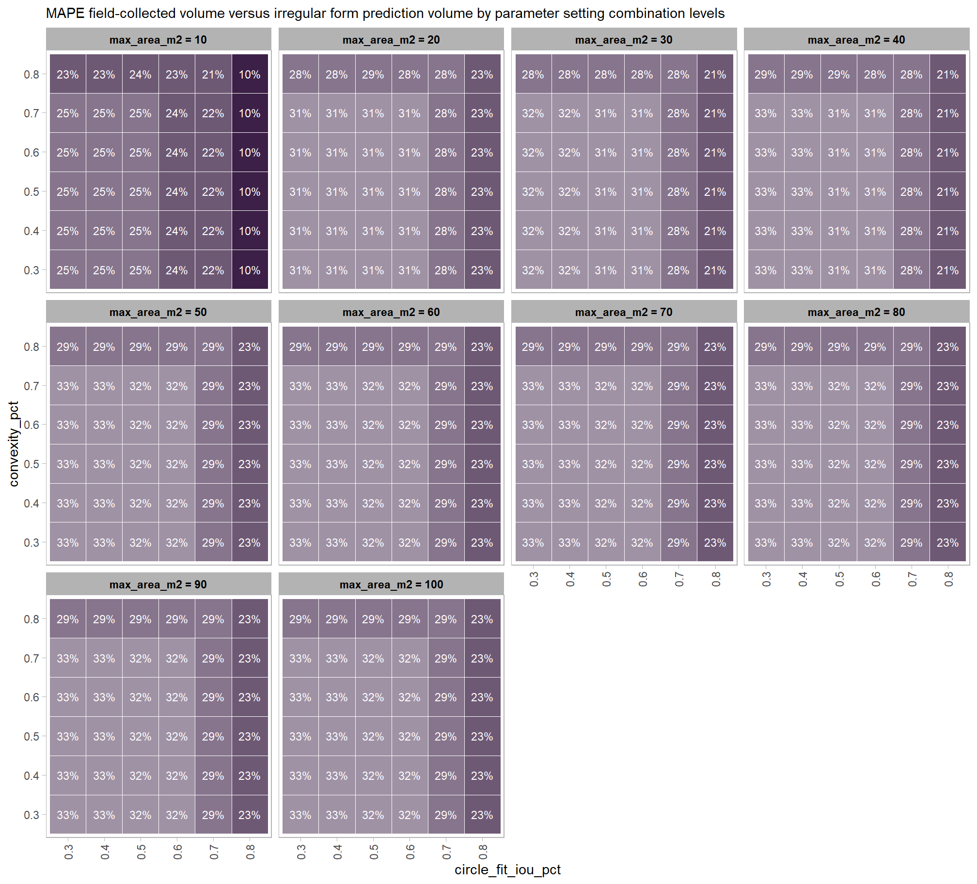
this plot allows for a simultaneous comparison of all metrics for pile detection and pile form quantification. it includes only the parameter combinations that achieved the best balanced accuracy, helping users identify the optimal settings by evaluating the trade-offs between detection and form quantification.
let’s table this
param_combos_ranked %>%
  dplyr::filter(is_final_selection) %>%
  dplyr::select(!tidyselect::contains("_pct_rank_")) %>%
  # first select to arrange eval_metric
  dplyr::select(
    ovrall_lab
    , max_ht_m,max_area_m2,convexity_pct,circle_fit_iou_pct,chm_res_m
    # detection
    , f_score, recall, precision
    # quantification
    , tidyselect::ends_with("_mean")
    , tidyselect::ends_with("_rmse")
    # , tidyselect::ends_with("_rrmse")
    , tidyselect::ends_with("_mape")
  ) %>%
  # second select to arrange pile_metric
  dplyr::select(
    ovrall_lab
    , max_ht_m,max_area_m2,convexity_pct,circle_fit_iou_pct,chm_res_m
    # detection
    , f_score, recall, precision
    # quantification
    , c(tidyselect::contains("volume") & !tidyselect::contains("paraboloid"))
    , tidyselect::contains("area")
    , tidyselect::contains("height")
    , tidyselect::contains("diameter")
  ) %>%
  # names()
  dplyr::mutate(
    dplyr::across(
      .cols = c(f_score, recall, precision, tidyselect::ends_with("_mape"))
      , .fn = ~ scales::percent(.x, accuracy = 1)
    )
    , dplyr::across(
      .cols = c(tidyselect::ends_with("_mean"))
      , .fn = ~ scales::comma(.x, accuracy = 0.01)
    )
    , dplyr::across(
      .cols = c(tidyselect::ends_with("_rmse"))
      , .fn = ~ scales::comma(.x, accuracy = 0.1)
    )
  ) %>%
  dplyr::mutate(blank= "   " ) %>%
  dplyr::relocate(blank, .before = f_score) %>%
  dplyr::arrange(desc(ovrall_lab)) %>%
  kableExtra::kbl(
    caption =
      paste0(
       "Structural Data Only"
       , "<br>pile detection and form quantification accuracy metrics for the top parameter settings tested"
       # , scales::percent(1-pct_rank_th_top,accuracy=1)
       , " (n="
       , scales::comma(n_th_top,accuracy=1)
       , ") "
       , "<br>based on both detection and quantification accuracy"
      )
    , col.names = c(
      ""
      ,"max_ht_m","max_area_m2","convexity_pct","circle_fit_iou_pct","chm_res_m"
      , "   "
      , "F-score", "Recall", "Precision"
      , rep(c("ME","RMSE","MAPE"), times = 3)
    )
    , escape = F
  ) %>%
  kableExtra::kable_styling(font_size = 11) %>%
  kableExtra::add_header_above(c(
    " "=7
    , "Detection" = 3
    , "Area" = 3
    , "Height" = 3
    , "Diameter" = 3
  )) %>%
  kableExtra::column_spec(seq(7,19,by=3), border_right = TRUE, include_thead = TRUE) %>%
  kableExtra::column_spec(
    column = 7:19
    , extra_css = "font-size: 10px;"
    , include_thead = T
  ) %>%
kableExtra::scroll_box(width = "740px") | max_ht_m | max_area_m2 | convexity_pct | circle_fit_iou_pct | chm_res_m | F-score | Recall | Precision | ME | RMSE | MAPE | ME | RMSE | MAPE | ME | RMSE | MAPE | ||
|---|---|---|---|---|---|---|---|---|---|---|---|---|---|---|---|---|---|---|
| 2:10:0.8:0.05:0.1 | 2 | 10 | 0.80 | 0.05 | 0.1 | 79% | 78% | 80% | -0.50 | 1.0 | 11% | -0.20 | 0.3 | 13% | 0.17 | 0.4 | 10% | |
| 2:20:0.8:0.05:0.1 | 2 | 20 | 0.80 | 0.05 | 0.1 | 81% | 82% | 80% | -0.60 | 1.7 | 11% | -0.24 | 0.4 | 13% | 0.18 | 0.5 | 11% | |
| 2:60:0.8:0.05:0.1 | 2 | 60 | 0.80 | 0.05 | 0.1 | 81% | 83% | 80% | -0.64 | 1.7 | 11% | -0.27 | 0.5 | 14% | 0.18 | 0.5 | 11% | |
| 2:50:0.8:0.05:0.1 | 2 | 50 | 0.80 | 0.05 | 0.1 | 81% | 83% | 80% | -0.64 | 1.7 | 11% | -0.27 | 0.5 | 14% | 0.18 | 0.5 | 11% | |
| 2:40:0.8:0.05:0.1 | 2 | 40 | 0.80 | 0.05 | 0.1 | 81% | 83% | 80% | -0.64 | 1.7 | 11% | -0.27 | 0.5 | 14% | 0.18 | 0.5 | 11% | |
| 2:30:0.8:0.05:0.1 | 2 | 30 | 0.80 | 0.05 | 0.1 | 81% | 83% | 80% | -0.64 | 1.7 | 11% | -0.27 | 0.5 | 14% | 0.18 | 0.5 | 11% | |
| 2:20:0.8:0.2:0.1 | 2 | 20 | 0.80 | 0.20 | 0.1 | 80% | 79% | 80% | -0.61 | 1.7 | 11% | -0.25 | 0.5 | 14% | 0.18 | 0.5 | 11% | |
| 2:60:0.8:0.2:0.1 | 2 | 60 | 0.80 | 0.20 | 0.1 | 80% | 81% | 80% | -0.65 | 1.7 | 11% | -0.27 | 0.5 | 14% | 0.19 | 0.5 | 11% | |
| 2:50:0.8:0.2:0.1 | 2 | 50 | 0.80 | 0.20 | 0.1 | 80% | 81% | 80% | -0.65 | 1.7 | 11% | -0.27 | 0.5 | 14% | 0.19 | 0.5 | 11% | |
| 2:40:0.8:0.2:0.1 | 2 | 40 | 0.80 | 0.20 | 0.1 | 80% | 81% | 80% | -0.65 | 1.7 | 11% | -0.27 | 0.5 | 14% | 0.19 | 0.5 | 11% | |
| 2:30:0.8:0.2:0.1 | 2 | 30 | 0.80 | 0.20 | 0.1 | 80% | 81% | 80% | -0.65 | 1.7 | 11% | -0.27 | 0.5 | 14% | 0.19 | 0.5 | 11% | |
| 2:30:0.65:0.5:0.1 | 2 | 30 | 0.65 | 0.50 | 0.1 | 75% | 78% | 72% | -0.64 | 1.8 | 11% | -0.25 | 0.4 | 14% | 0.19 | 0.5 | 11% |
what is the expected detection accuracy of the top 12 settings?
plt_detection_dist(
  df = param_combos_ranked %>% dplyr::filter(is_final_selection) %>% dplyr::select(!tidyselect::contains("_pct_rank_"))
  , paste0(
    "Structural Data Only"
    , "\ndistribution of pile detection metrics for the top parameter settings tested"
    , " (n="
    , scales::comma(n_th_top,accuracy=1)
    , ") "
    , "\nbased on both detection and quantification accuracy"
  )
)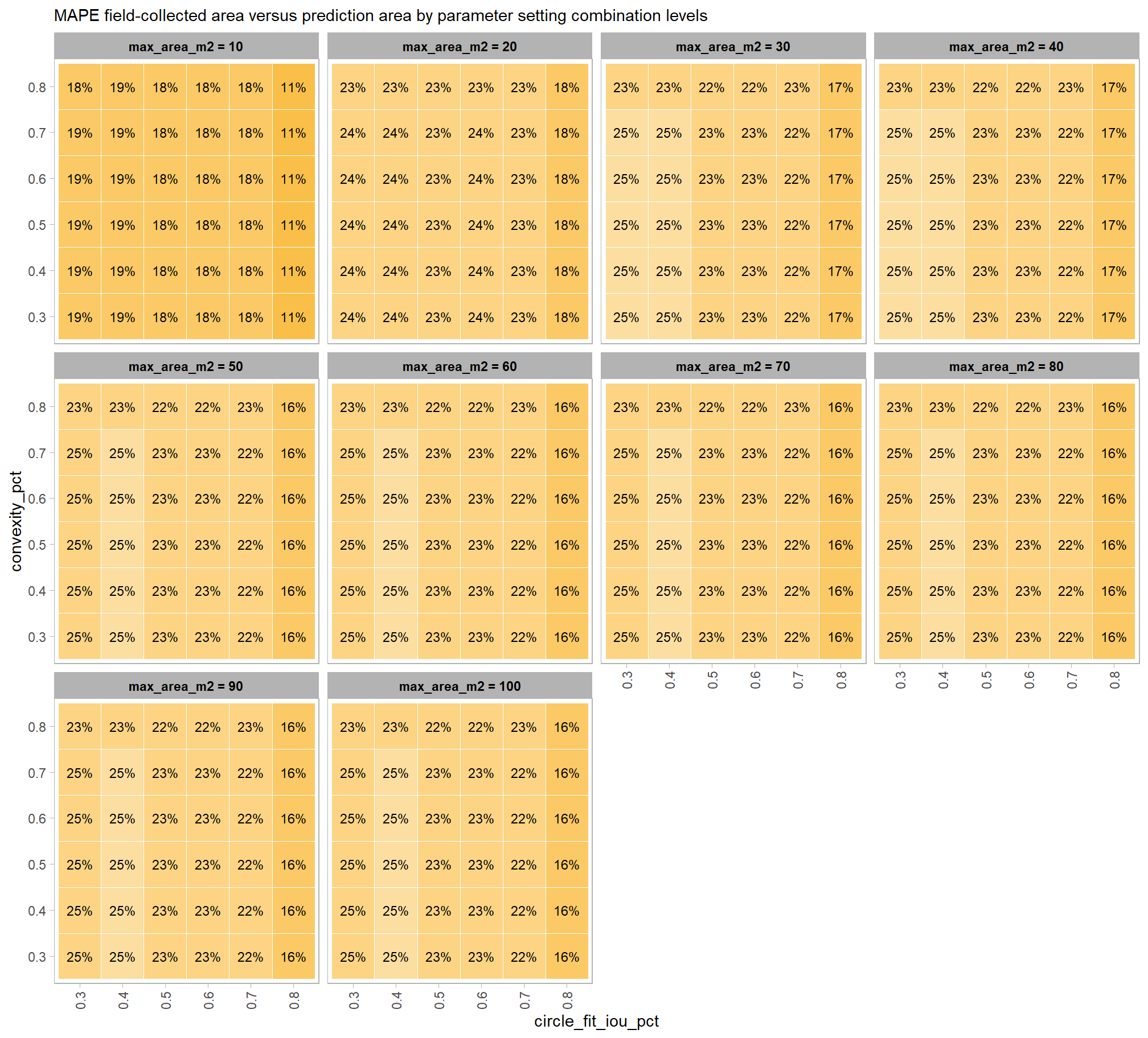
what is the expected quantification accuracy of the top 12 settings?
# plot it
plt_form_quantification_dist(
  df = param_combos_ranked %>% dplyr::filter(is_final_selection) %>% dplyr::select(!tidyselect::contains("_pct_rank_"))
  , paste0(
    "Structural Data Only"
    , "\ndistribution of pile form quantification metrics for the top parameter settings tested"
    , " (n="
    , scales::comma(n_th_top,accuracy=1)
    , ") "
    , "\nbased on both detection and quantification accuracy"
  )
)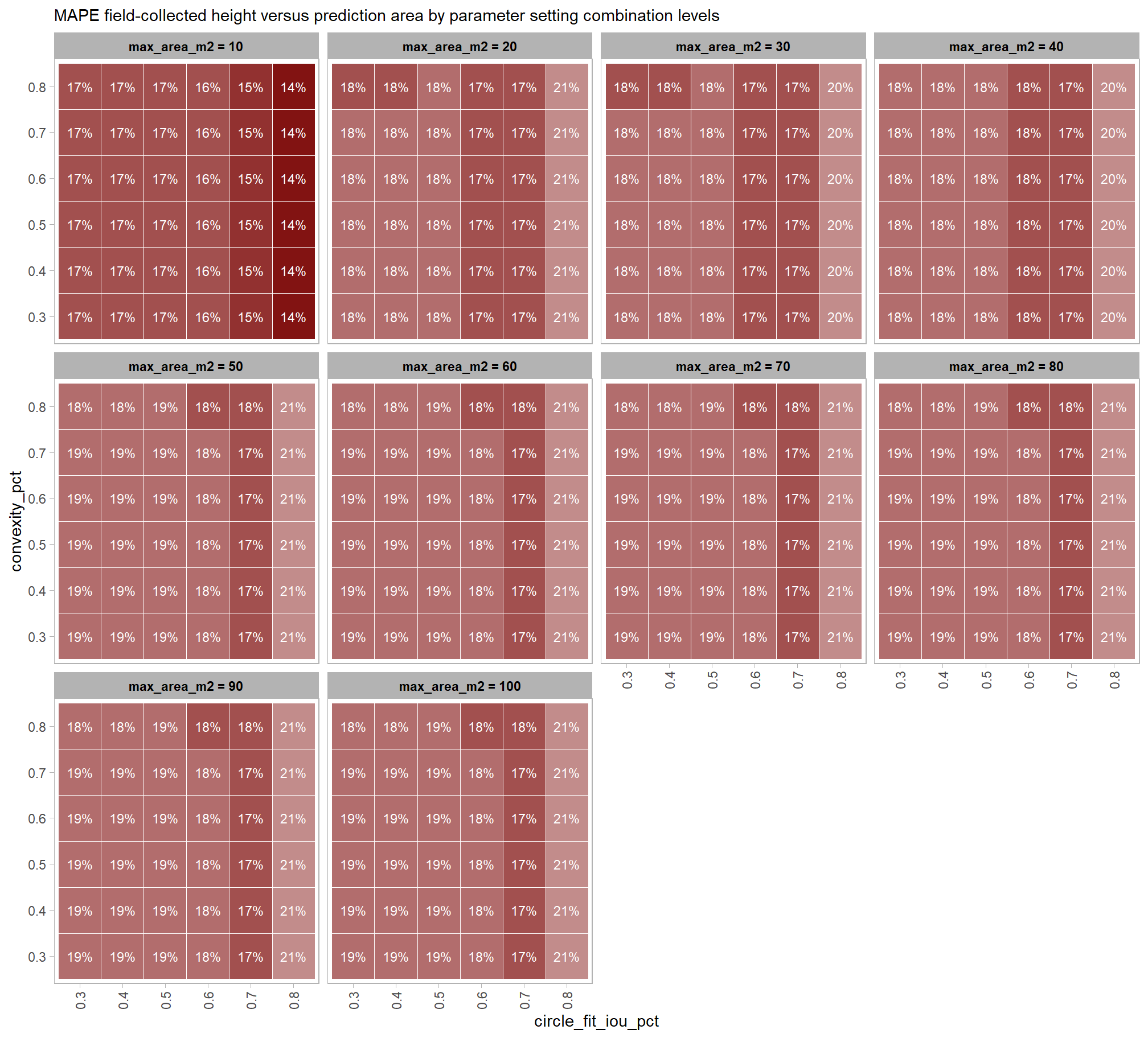
finally, here are the combinations selected compared against all 5,880 combinations tested.
param_combos_ranked %>%
  dplyr::select(
    rn,max_ht_m,max_area_m2,convexity_pct,circle_fit_iou_pct
    , is_final_selection
    , f_score, precision, recall
    # quantification accuracy
    , tidyselect::ends_with("_mape")
  ) %>%
  tidyr::pivot_longer(
    cols = c(
      tidyselect::ends_with("_mape")
      # ,precision,recall
    )
    , names_to = "metric"
    , values_to = "value"
  ) %>%
  dplyr::mutate(
    eval_metric = stringr::str_extract(metric, "(_rmse|_rrmse|_mean|_mape)$") %>%
      stringr::str_remove_all("_") %>%
      stringr::str_replace_all("mean","me") %>%
      toupper() %>%
      factor(
        ordered = T
        , levels = c("ME","RMSE","RRMSE","MAPE")
      )
    , pile_metric = metric %>%
      stringr::str_remove("(_rmse|_rrmse|_mean|_mape)$") %>%
      stringr::str_extract("(paraboloid_volume|volume|area|height|diameter|precision|recall)") %>%
      factor(
        ordered = T
        , levels = c(
          "volume"
          , "paraboloid_volume"
          , "area"
          , "height"
          , "diameter"
          , "recall"
          , "precision"
        )
        , labels = c(
          "Volume"
          , "Volume paraboloid"
          , "Area (m2)"
          , "Height (m)"
          , "Diameter (m)"
          , "Recall"
          , "Precision"
        )
      )
    , color_metric = ifelse(is_final_selection, pile_metric, NA) %>% factor()
  ) %>%
  dplyr::arrange(is_final_selection) %>%
  # plot
  ggplot2::ggplot(mapping = ggplot2::aes(x = f_score, y = value, color = color_metric)) +
  ggplot2::geom_point() +
  ggplot2::facet_wrap(facets = dplyr::vars(pile_metric)) +
  harrypotter::scale_color_hp_d(option = "hermionegranger", na.value = "gray88") +
  ggplot2::scale_x_continuous(
    labels = scales::percent_format(accuracy = 1)
    , limits = c(0,1)
  ) +
  ggplot2::scale_y_continuous(
    labels = scales::percent_format(accuracy = 1)
    , limits = c(0,NA)
  ) +
  ggplot2::labs(x = "F-Score", y = "MAPE", caption = "*records in gray not selected") +
  ggplot2::theme_light() +
  ggplot2::theme(
    legend.position = "none"
    , strip.text = ggplot2::element_text(size = 11, color = "black", face = "bold")
  )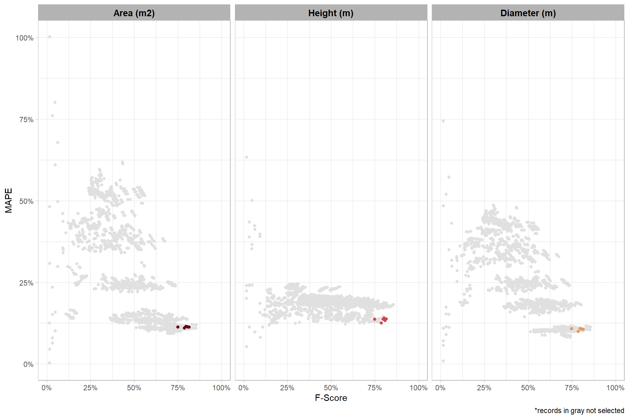
8.5.3.2 by CHM resolution
To select the best-performing parameter combinations of those tested, we will prioritize those that balance detection and quantification accuracy. From this group, we will then identify the settings that achieve the highest pile detection rates (recall). These recommendations are for users who are working with a CHM with a resolution in the range of those tested for this analysis or can aggregate (i.e. make more coarse) a CHM to a resolution tested for the purpose of either improving processing performance or enhancing pile detection and/or quantification accuracy based on the results shown here
we already created this data above (param_combos_ranked) using the F-Score and the average rank of the MAPE metrics across all form measurements (i.e. height, diameter, area) to determine the best overall list by CHM resolution
8.5.3.2.1 Top 2.0%
let’s check out the parameter settings of the top 2.0% (n=23) from all 1,176 combinations tested by CHM resolution. these are “votes” for the parameter setting based on the combinations that achieved the best balance between both detection and quantification accuracy.
param_combos_ranked %>%
  dplyr::filter(is_top_chm) %>%
  dplyr::select(tidyselect::contains("f_score"), max_ht_m,max_area_m2,convexity_pct,circle_fit_iou_pct,chm_res_m,chm_res_m_desc) %>%
  tidyr::pivot_longer(
    cols = c(max_ht_m,max_area_m2,convexity_pct,circle_fit_iou_pct)
    , names_to = "metric"
    , values_to = "value"
  ) %>%
  dplyr::count(chm_res_m,chm_res_m_desc, metric, value) %>%
  dplyr::group_by(chm_res_m,chm_res_m_desc, metric) %>%
  dplyr::mutate(
    pct=n/sum(n)
    , lab = paste0(scales::percent(pct,accuracy=0.1)) #, "\nn=", scales::comma(n,accuracy=1))
  ) %>%
  ggplot2::ggplot(
    mapping = ggplot2::aes(x = factor(value), y=pct, label=lab, fill = metric)
  ) +
  ggplot2::geom_col(width = 0.6) +
  ggplot2::geom_text(color = "black", size = 2.2, vjust = -0.2) +
  ggplot2::facet_grid(cols = dplyr::vars(metric), rows = dplyr::vars(chm_res_m_desc), scales = "free_x") +
  ggplot2::scale_y_continuous(
    breaks = seq(0,1,by=0.2)
    , labels = scales::percent
    , expand = ggplot2::expansion(mult = c(0,0.2))
  ) +
  ggplot2::scale_fill_manual(values = pal_param[1:4]) +
  ggplot2::labs(
    x = "parameter setting", y = ""
    , fill = ""
    , subtitle = paste0(
      "Structural Data Only"
       , "\nparameter settings of top "
       , scales::percent(pct_th_top_chm,accuracy=0.1)
       , " (n="
       , scales::comma(n_combos_top_chm , accuracy = 1)
       , ") "
       , "parameter combinations tested by CHM resolution\nbased on both detection and quantification accuracy"
    )
  ) +
  ggplot2::theme_light() +
  ggplot2::theme(
    legend.position = "none"
    , strip.text.x = ggplot2::element_text(size = 11, color = "black", face = "bold")
    , strip.text.y = ggplot2::element_text(size = 9, color = "black", face = "bold")
    , axis.text.y = ggplot2::element_text(size = 6)
    , axis.text.x = ggplot2::element_text(size = 8)
    , plot.subtitle = ggplot2::element_text(size = 8)
  )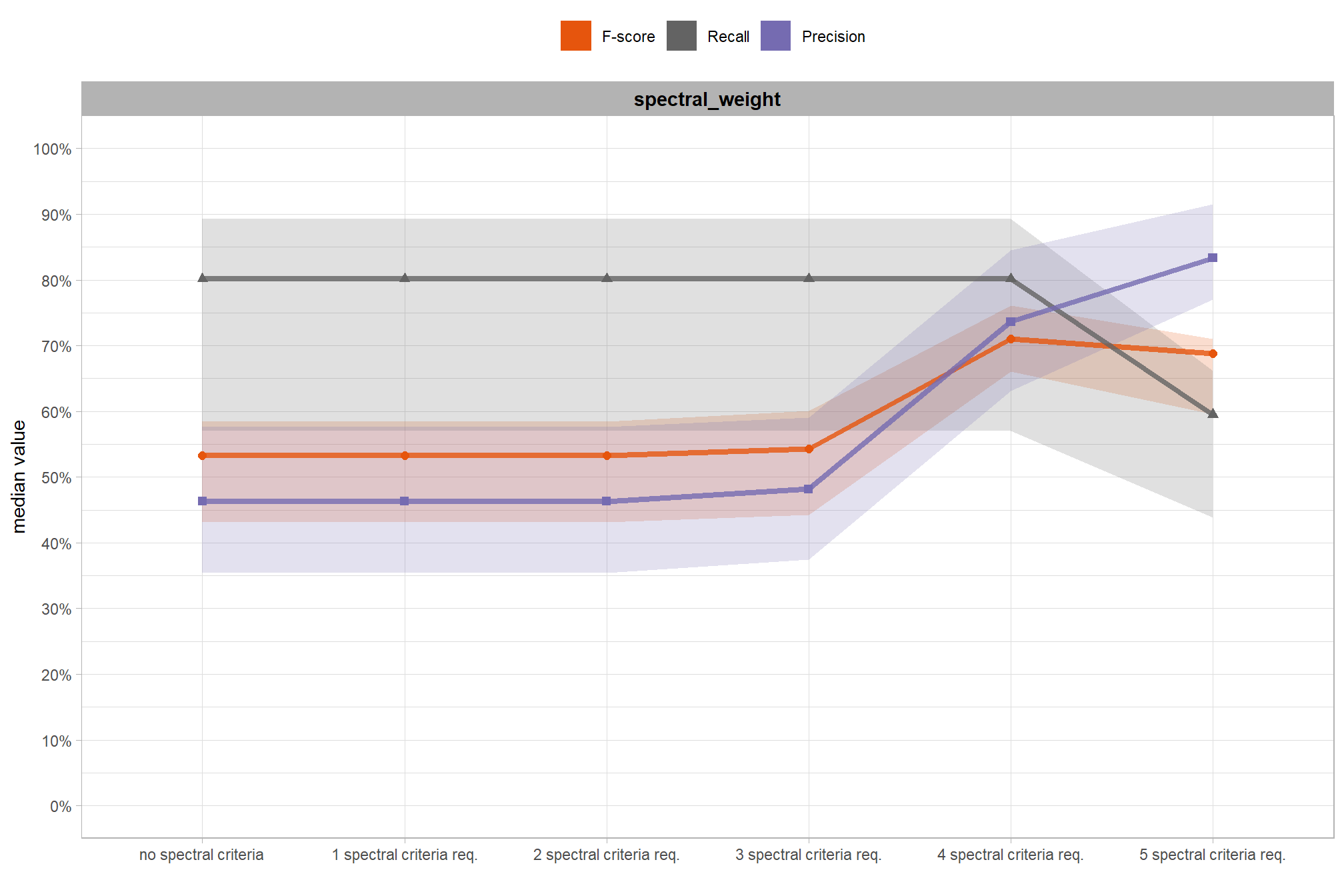
what is the expected detection accuracy of the top 2.0% (n=23) combinations tested by CHM resolution?
plt_detection_dist2(
  df = param_combos_ranked %>% dplyr::filter(is_top_chm) %>% dplyr::select(!tidyselect::contains("_pct_rank_"))
  , paste0(
    "Structural Data Only"
    , "\ndistribution of pile detection metrics for top "
    , scales::percent(pct_th_top_chm,accuracy=0.1)
    , " (n="
    , scales::comma(n_combos_top_chm, accuracy=1)
    , ") "
    , "parameter combinations tested by CHM resolution\nbased on both detection and quantification accuracy"
  )
)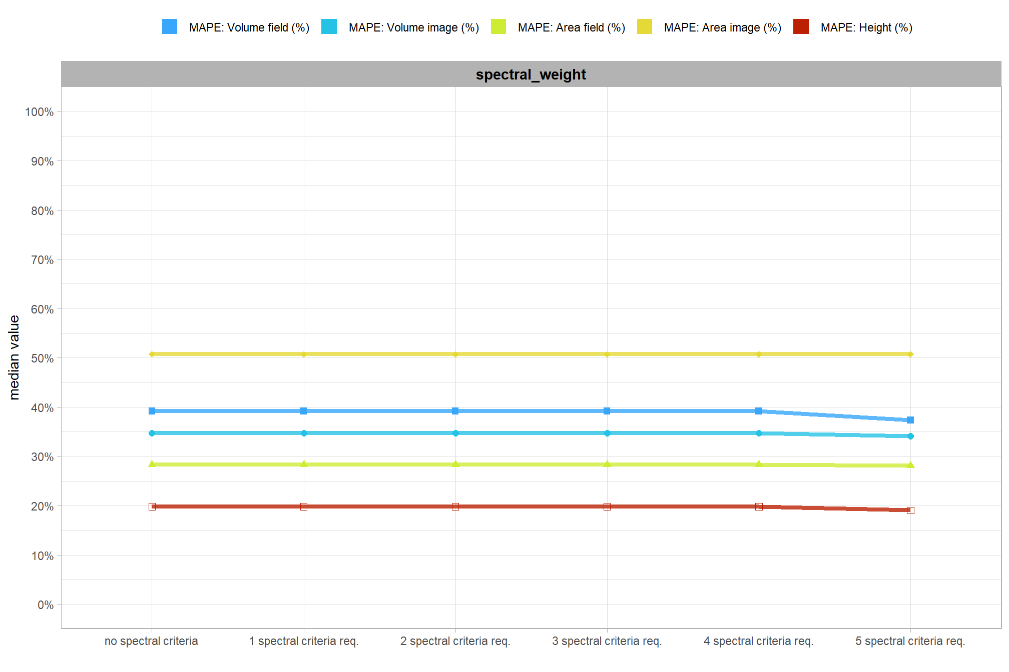
what is the expected MAPE of the top 2.0% (n=23) combinations tested by CHM resolution?
# plot it
plt_form_quantification_dist2(
  df = param_combos_ranked %>% dplyr::filter(is_top_chm) %>% dplyr::select(!tidyselect::contains("_pct_rank_"))
  , quant_metric = "mape"
  , paste0(
    "Structural Data Only"
    , "\ndistribution of pile form quantification metrics for the top "
    , scales::percent(pct_th_top_chm,accuracy=0.1)
    , " (n="
    , scales::comma(n_combos_top_chm, accuracy=1)
    , ") "
    , "parameter combinations tested by CHM resolution\nbased on both detection and quantification accuracy"
  )
)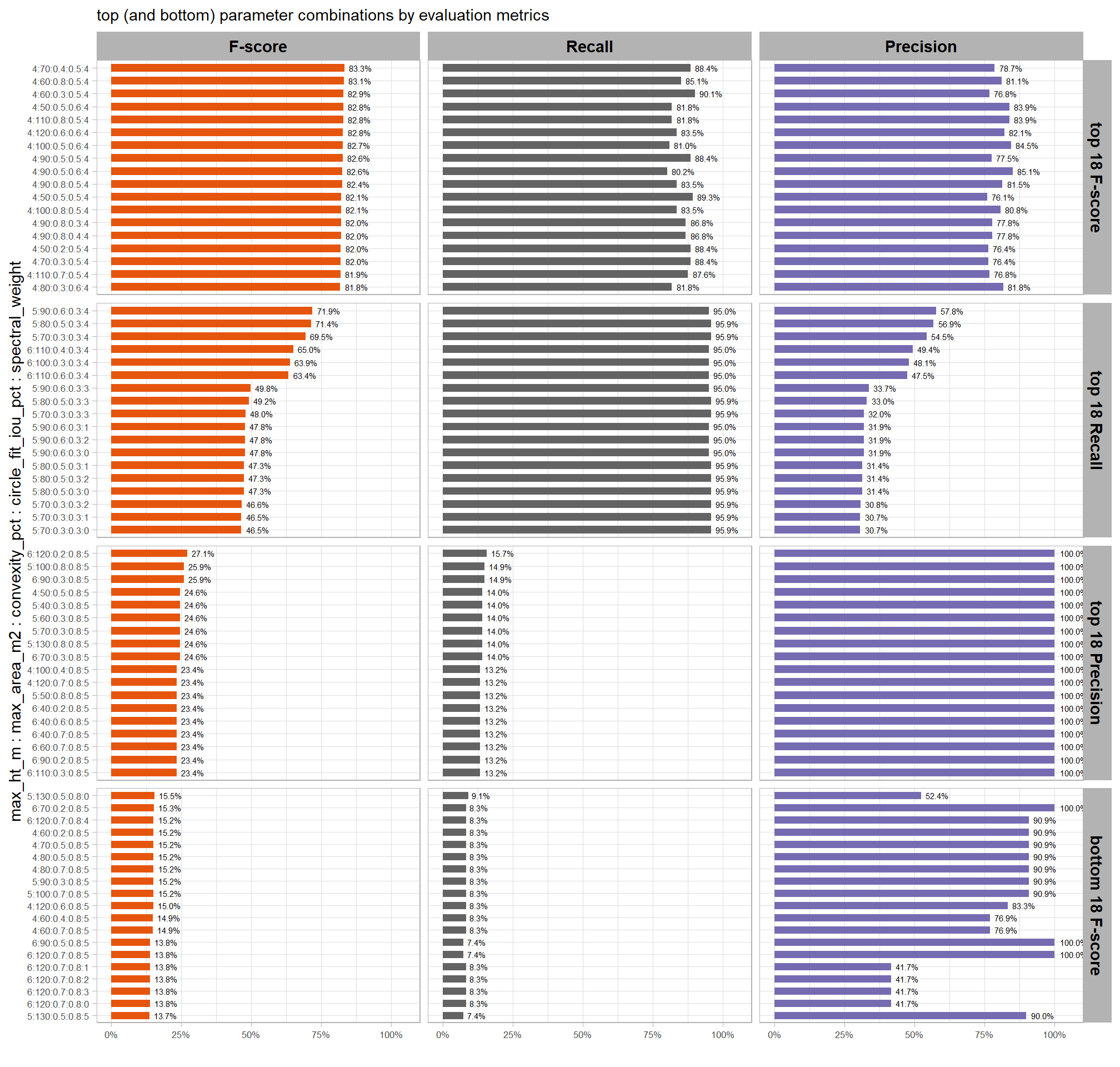
what is the expected Mean Error (ME) of the top 2.0% (n=23) combinations tested by CHM resolution?
# plot it
plt_form_quantification_dist2(
  df = param_combos_ranked %>% dplyr::filter(is_top_chm) %>% dplyr::select(!tidyselect::contains("_pct_rank_"))
  , quant_metric = "mean"
  , paste0(
    "Structural Data Only"
    , "\ndistribution of pile form quantification metrics for the top "
    , scales::percent(pct_th_top_chm,accuracy=0.1)
    , " (n="
    , scales::comma(n_combos_top_chm, accuracy=1)
    , ") "
    , "parameter combinations tested by CHM resolution\nbased on both detection and quantification accuracy"
  )
)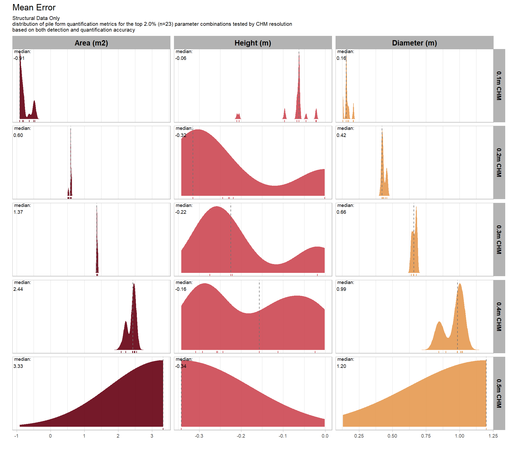
what is the expected RMSE of the top 2.0% (n=23) combinations tested by CHM resolution?
# plot it
plt_form_quantification_dist2(
  df = param_combos_ranked %>% dplyr::filter(is_top_chm) %>% dplyr::select(!tidyselect::contains("_pct_rank_"))
  , quant_metric = "rmse"
  , paste0(
    "Structural Data Only"
    , "\ndistribution of pile form quantification metrics for the top "
    , scales::percent(pct_th_top_chm,accuracy=0.1)
    , " (n="
    , scales::comma(n_combos_top_chm, accuracy=1)
    , ") "
    , "parameter combinations tested by CHM resolution\nbased on both detection and quantification accuracy"
  )
)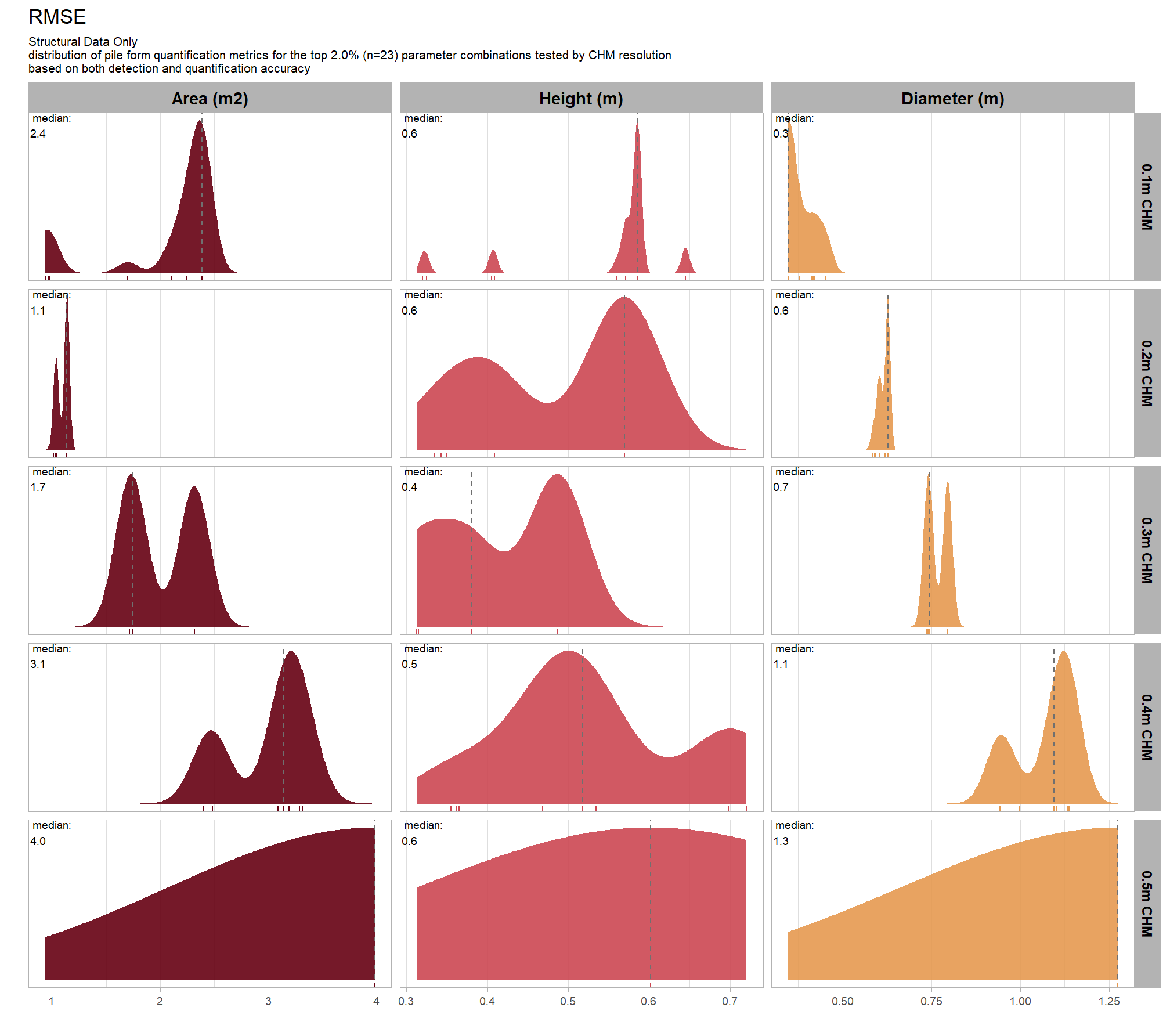
8.5.3.2.2 Top 6 settings
Let’s focus on the top 6 parameter settings tested by CHM resolution to highlight the pile detection and form quantification accuracies achieved by these settings
# pal_temp %>% scales::show_col()
# filter and reshape
param_combos_ranked %>%
  dplyr::filter(is_final_selection_chm) %>%
  dplyr::select(!tidyselect::contains("_pct_rank_")) %>%
  dplyr::select(
    max_ht_m,max_area_m2,convexity_pct,circle_fit_iou_pct,chm_res_m,chm_res_m_desc
    , chm_lab
    # detection
    , f_score, recall, precision
    # quantification
    , tidyselect::ends_with("_rmse")
    , tidyselect::ends_with("_rrmse")
    , tidyselect::ends_with("_mean")
    , tidyselect::ends_with("_mape")
  ) %>%
  tidyr::pivot_longer(
    cols = c(
      f_score, recall, precision
      , tidyselect::ends_with("_rmse")
      , tidyselect::ends_with("_rrmse")
      , tidyselect::ends_with("_mean")
      , tidyselect::ends_with("_mape")
    )
    , names_to = "metric"
    , values_to = "value"
  ) %>%
  dplyr::mutate(
    eval_metric = stringr::str_extract(metric, "(_rmse|_rrmse|_mean|_mape|f_score|recall|precision)$") %>%
      stringr::str_remove_all("_") %>%
      stringr::str_replace_all("mean","me") %>%
      toupper() %>%
      factor(
        ordered = T
        , levels = c("FSCORE","RECALL","PRECISION", "ME","RMSE","RRMSE","MAPE")
        , labels = c("F-score","Recall","Precision", "ME","RMSE","RRMSE","MAPE")
      )
    , pile_metric = metric %>%
      stringr::str_remove("(_rmse|_rrmse|_mean|_mape)$") %>%
      stringr::str_extract("(paraboloid_volume|volume|area|height|diameter)") %>%
      dplyr::coalesce("detection") %>%
      factor(
        ordered = T
        , levels = c(
          "detection"
          , "volume"
          , "paraboloid_volume"
          , "area"
          , "height"
          , "diameter"
        )
        , labels = c(
          "Detection"
          , "Volume"
          , "Volume paraboloid"
          , "Area (m2)"
          , "Height (m)"
          , "Diameter (m)"
        )
      )
    , value_lab = dplyr::case_when(
        eval_metric %in% c("F-score","Recall","Precision", "RRMSE", "MAPE") ~ scales::percent(value,accuracy=0.1)
        , eval_metric == "ME" ~ scales::comma(value,accuracy=0.01)
        , T ~ scales::comma(value,accuracy=0.1)
      )
  ) %>%
  # make var for color
  dplyr::group_by(chm_res_m,chm_res_m_desc, pile_metric, eval_metric) %>%
  dplyr::mutate(
    # for ME, color by abs...for f-score,recall,precision color by -value so that higher means better...
      # ...since higher means worse for quantification accuracy metrics
    value_dir = dplyr::case_when(
      eval_metric %in% c("ME") ~ abs(value)
      , eval_metric %in% c("F-score","Recall","Precision") ~ -value
      , T ~ value
    )
    , value_z = (value_dir-mean(value_dir,na.rm=T))/sd(value_dir,na.rm=T) # this is the key to the different colors within facets
  ) %>%
  dplyr::ungroup() %>%
  dplyr::filter(!eval_metric %in% c("RRMSE")) %>%
  # View()
  ggplot2::ggplot(mapping = ggplot2::aes(x = eval_metric, y = chm_lab)) +
  ggplot2::geom_tile(
    mapping = ggplot2::aes(fill = pile_metric, alpha = -value_z)
    , color = "gray"
  ) +
  ggplot2::geom_text(
    mapping = ggplot2::aes(label = value_lab, fontface = "bold")
    , color = "white"
    , size = 3
  ) +
  ggplot2::facet_grid(cols = dplyr::vars(pile_metric), rows = dplyr::vars(chm_res_m_desc), scales = "free") +
  ggplot2::scale_x_discrete(position = "top") +
  ggplot2::scale_fill_manual(values = c("gray33", harrypotter::hp(n=3,option = "hermionegranger") )) +
  ggplot2::scale_alpha_binned(range = c(0.55, 1)) + # this is the key to the different colors within facets
  ggplot2::theme_light() +
  ggplot2::labs(
    x = ""
    , y = "max_ht_m : max_area_m2 : convexity_pct : circle_fit_iou_pct : chm_res_m"
    , subtitle = paste0(
       "Structural Data Only"
       , "\npile detection and form quantification accuracy metrics for the top parameter settings tested"
       # , scales::percent(1-pct_rank_th_top,accuracy=1)
       , " (n="
       , scales::comma(n_th_top_chm,accuracy=1)
       , ") by CHM resolution"
       , "\nbased on both detection and quantification accuracy"
      )
    , caption = "*darker colors indicate relatively higher accuracy values"
  ) +
  ggplot2::theme(
    legend.position = "none"
    , panel.grid = ggplot2::element_blank()
    , strip.placement = "outside"
    , strip.text.x = ggplot2::element_text(size = 8, color = "black", face = "bold")
    , strip.text.y = ggplot2::element_text(size = 9, color = "black", face = "bold")
    , axis.text.x = ggplot2::element_text(size = 7, color = "black", face = "bold")
    , axis.text.y = ggplot2::element_text(size = 7)
    , axis.title.x = ggplot2::element_blank()
    , plot.subtitle = ggplot2::element_text(size = 8)
  )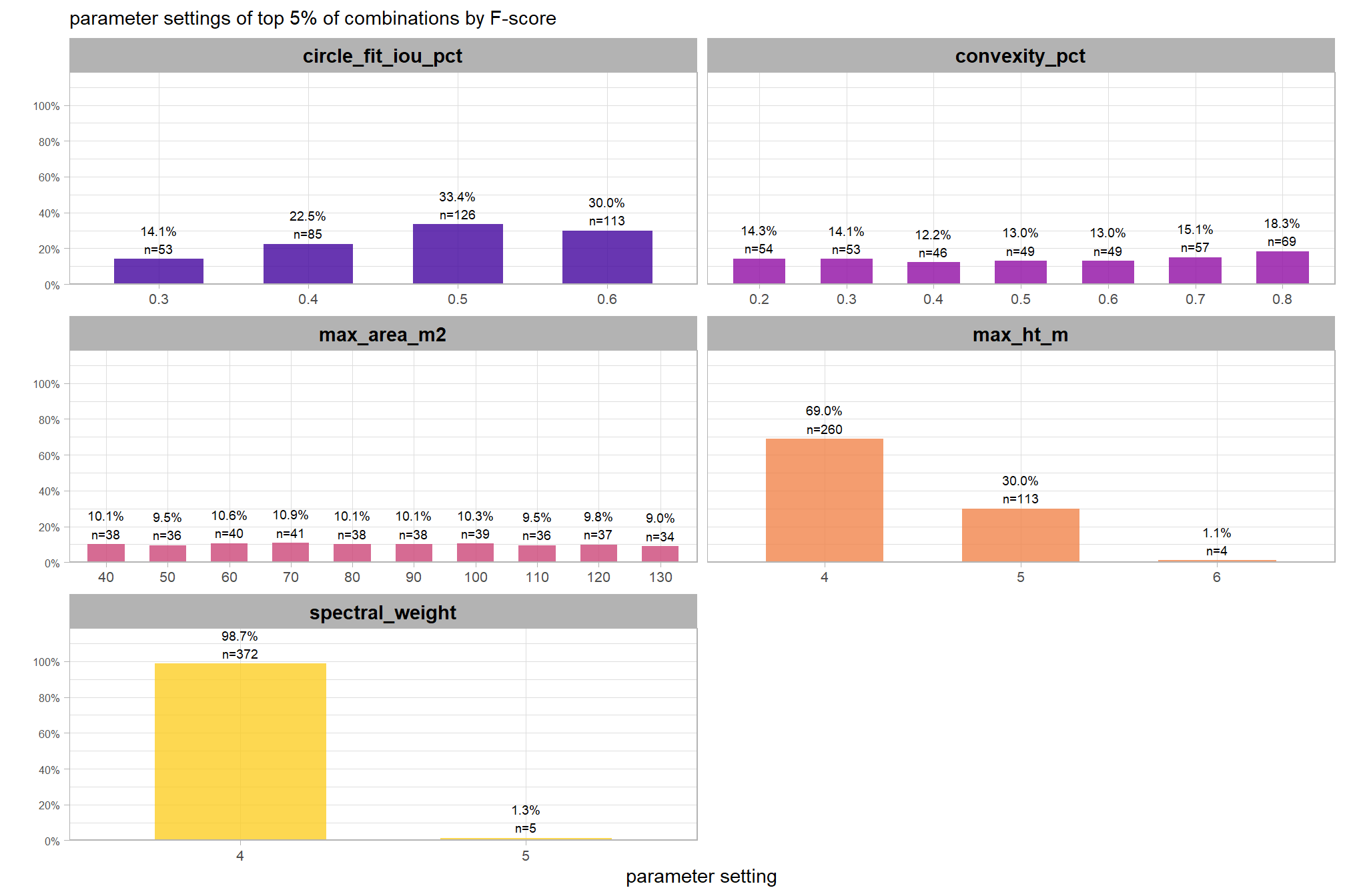
this plot allows for a simultaneous comparison of all metrics for pile detection and pile form quantification. it includes only the parameter combinations of those tested that achieved the best balanced accuracy, helping users identify the optimal settings by evaluating the trade-offs between detection and form quantification.
let’s table this
param_combos_ranked %>%
  dplyr::filter(is_final_selection_chm) %>%
  dplyr::select(!tidyselect::contains("_pct_rank_")) %>%
  # first select to arrange eval_metric
  dplyr::select(
    chm_lab, chm_res_m_desc
    , max_ht_m,max_area_m2,convexity_pct,circle_fit_iou_pct,chm_res_m
    # detection
    , f_score, recall, precision
    # quantification
    , tidyselect::ends_with("_mean")
    , tidyselect::ends_with("_rmse")
    # , tidyselect::ends_with("_rrmse")
    , tidyselect::ends_with("_mape")
  ) %>%
  # second select to arrange pile_metric
  dplyr::select(
    chm_lab, chm_res_m_desc
    , max_ht_m,max_area_m2,convexity_pct,circle_fit_iou_pct,chm_res_m
    # detection
    , f_score, recall, precision
    # quantification
    , c(tidyselect::contains("volume") & !tidyselect::contains("paraboloid"))
    , tidyselect::contains("area")
    , tidyselect::contains("height")
    , tidyselect::contains("diameter")
  ) %>%
  # names()
  dplyr::mutate(
    dplyr::across(
      .cols = c(f_score, recall, precision, tidyselect::ends_with("_mape"))
      , .fn = ~ scales::percent(.x, accuracy = 1)
    )
    , dplyr::across(
      .cols = c(tidyselect::ends_with("_mean"))
      , .fn = ~ scales::comma(.x, accuracy = 0.01)
    )
    , dplyr::across(
      .cols = c(tidyselect::ends_with("_rmse"))
      , .fn = ~ scales::comma(.x, accuracy = 0.1)
    )
  ) %>%
  dplyr::mutate(blank= "   " ) %>%
  dplyr::relocate(blank, .before = f_score) %>%
  dplyr::arrange(chm_res_m, desc(chm_lab)) %>%
  dplyr::select(-chm_res_m) %>%
  dplyr::relocate(chm_res_m_desc) %>%
  kableExtra::kbl(
    caption =
      paste0(
       "Structural Data Only"
       , "<br>pile detection and form quantification accuracy metrics for the top parameter settings tested"
       # , scales::percent(1-pct_rank_th_top,accuracy=1)
       , " (n="
       , scales::comma(n_th_top_chm,accuracy=1)
       , ") by CHM resolution "
       , "<br>based on both detection and quantification accuracy"
      )
    , col.names = c(
      ".", ""
      ,"max_ht_m","max_area_m2","convexity_pct","circle_fit_iou_pct"
      , "   "
      , "F-score", "Recall", "Precision"
      , rep(c("ME","RMSE","MAPE"), times = 3)
    )
    , escape = F
  ) %>%
  kableExtra::kable_styling(font_size = 11) %>%
  kableExtra::add_header_above(c(
    " "=7
    , "Detection" = 3
    # , "Volume" = 3
    , "Area" = 3
    , "Height" = 3
    , "Diameter" = 3
  )) %>%
  kableExtra::column_spec(seq(7,19,by=3), border_right = TRUE, include_thead = TRUE) %>%
  kableExtra::column_spec(
    column = 7:19
    , extra_css = "font-size: 10px;"
    , include_thead = T
  ) %>%
  kableExtra::collapse_rows(columns = 1, valign = "top") %>%
kableExtra::scroll_box(width = "740px") | . | max_ht_m | max_area_m2 | convexity_pct | circle_fit_iou_pct | F-score | Recall | Precision | ME | RMSE | MAPE | ME | RMSE | MAPE | ME | RMSE | MAPE | ||
|---|---|---|---|---|---|---|---|---|---|---|---|---|---|---|---|---|---|---|
| 0.1m CHM | 2:10:0.8:0.05:0.1 | 2 | 10 | 0.80 | 0.05 | 79% | 78% | 80% | -0.50 | 1.0 | 11% | -0.20 | 0.3 | 13% | 0.17 | 0.4 | 10% | |
| 3:10:0.8:0.35:0.1 | 3 | 10 | 0.80 | 0.35 | 77% | 79% | 75% | -0.46 | 0.9 | 11% | -0.02 | 0.4 | 17% | 0.17 | 0.4 | 10% | ||
| 5:60:0.8:0.65:0.1 | 5 | 60 | 0.80 | 0.65 | 76% | 90% | 66% | -0.80 | 2.1 | 10% | -0.10 | 0.6 | 18% | 0.21 | 0.5 | 10% | ||
| 5:50:0.8:0.65:0.1 | 5 | 50 | 0.80 | 0.65 | 76% | 90% | 66% | -0.80 | 2.1 | 10% | -0.10 | 0.6 | 18% | 0.21 | 0.5 | 10% | ||
| 5:40:0.8:0.65:0.1 | 5 | 40 | 0.80 | 0.65 | 75% | 88% | 66% | -0.63 | 1.7 | 10% | -0.05 | 0.6 | 18% | 0.21 | 0.5 | 10% | ||
| 3:10:0.8:0.5:0.1 | 3 | 10 | 0.80 | 0.50 | 77% | 77% | 78% | -0.46 | 0.9 | 11% | -0.02 | 0.4 | 17% | 0.17 | 0.4 | 10% | ||
| 0.2m CHM | 2:10:0.8:0.05:0.2 | 2 | 10 | 0.80 | 0.05 | 70% | 74% | 66% | 0.53 | 1.0 | 12% | -0.22 | 0.3 | 13% | 0.43 | 0.6 | 16% | |
| 2:10:0.8:0.2:0.2 | 2 | 10 | 0.80 | 0.20 | 68% | 69% | 67% | 0.52 | 1.0 | 12% | -0.23 | 0.3 | 14% | 0.42 | 0.6 | 16% | ||
| 3:10:0.8:0.65:0.2 | 3 | 10 | 0.80 | 0.65 | 73% | 68% | 80% | 0.62 | 1.0 | 13% | 0.00 | 0.4 | 17% | 0.46 | 0.6 | 17% | ||
| 3:10:0.35:0.65:0.2 | 3 | 10 | 0.35 | 0.65 | 73% | 68% | 79% | 0.62 | 1.0 | 13% | 0.00 | 0.4 | 17% | 0.46 | 0.6 | 17% | ||
| 3:10:0.2:0.65:0.2 | 3 | 10 | 0.20 | 0.65 | 73% | 68% | 79% | 0.62 | 1.0 | 13% | 0.00 | 0.4 | 17% | 0.46 | 0.6 | 17% | ||
| 3:10:0.05:0.65:0.2 | 3 | 10 | 0.05 | 0.65 | 73% | 68% | 79% | 0.62 | 1.0 | 13% | 0.00 | 0.4 | 17% | 0.46 | 0.6 | 17% | ||
| 0.3m CHM | 3:10:0.8:0.65:0.3 | 3 | 10 | 0.80 | 0.65 | 65% | 67% | 63% | 1.40 | 1.7 | 23% | -0.02 | 0.4 | 16% | 0.64 | 0.7 | 23% | |
| 3:10:0.65:0.65:0.3 | 3 | 10 | 0.65 | 0.65 | 65% | 67% | 62% | 1.40 | 1.7 | 23% | -0.02 | 0.4 | 16% | 0.64 | 0.7 | 23% | ||
| 3:10:0.5:0.65:0.3 | 3 | 10 | 0.50 | 0.65 | 65% | 67% | 62% | 1.40 | 1.7 | 23% | -0.02 | 0.4 | 16% | 0.64 | 0.7 | 23% | ||
| 3:10:0.35:0.65:0.3 | 3 | 10 | 0.35 | 0.65 | 65% | 67% | 62% | 1.40 | 1.7 | 23% | -0.02 | 0.4 | 16% | 0.64 | 0.7 | 23% | ||
| 3:10:0.2:0.65:0.3 | 3 | 10 | 0.20 | 0.65 | 65% | 67% | 62% | 1.40 | 1.7 | 23% | -0.02 | 0.4 | 16% | 0.64 | 0.7 | 23% | ||
| 3:10:0.05:0.65:0.3 | 3 | 10 | 0.05 | 0.65 | 65% | 67% | 62% | 1.40 | 1.7 | 23% | -0.02 | 0.4 | 16% | 0.64 | 0.7 | 23% | ||
| 0.4m CHM | 2:20:0.8:0.05:0.4 | 2 | 20 | 0.80 | 0.05 | 55% | 79% | 42% | 2.43 | 3.1 | 37% | -0.24 | 0.4 | 14% | 1.02 | 1.1 | 34% | |
| 2:60:0.8:0.05:0.4 | 2 | 60 | 0.80 | 0.05 | 56% | 81% | 42% | 2.48 | 3.1 | 37% | -0.29 | 0.5 | 15% | 1.01 | 1.1 | 34% | ||
| 2:50:0.8:0.05:0.4 | 2 | 50 | 0.80 | 0.05 | 56% | 81% | 42% | 2.48 | 3.1 | 37% | -0.29 | 0.5 | 15% | 1.01 | 1.1 | 34% | ||
| 2:40:0.8:0.05:0.4 | 2 | 40 | 0.80 | 0.05 | 56% | 81% | 42% | 2.48 | 3.1 | 37% | -0.29 | 0.5 | 15% | 1.01 | 1.1 | 34% | ||
| 2:30:0.8:0.05:0.4 | 2 | 30 | 0.80 | 0.05 | 56% | 81% | 42% | 2.48 | 3.1 | 37% | -0.29 | 0.5 | 15% | 1.01 | 1.1 | 34% | ||
| 2:30:0.8:0.2:0.4 | 2 | 30 | 0.80 | 0.20 | 54% | 75% | 42% | 2.50 | 3.2 | 37% | -0.31 | 0.5 | 15% | 1.01 | 1.1 | 34% | ||
| 0.5m CHM | 2:60:0.8:0.65:0.5 | 2 | 60 | 0.80 | 0.65 | 42% | 34% | 54% | 3.33 | 4.0 | 49% | -0.34 | 0.6 | 17% | 1.20 | 1.3 | 39% | |
| 2:50:0.8:0.65:0.5 | 2 | 50 | 0.80 | 0.65 | 42% | 34% | 54% | 3.33 | 4.0 | 49% | -0.34 | 0.6 | 17% | 1.20 | 1.3 | 39% | ||
| 2:40:0.8:0.65:0.5 | 2 | 40 | 0.80 | 0.65 | 42% | 34% | 54% | 3.33 | 4.0 | 49% | -0.34 | 0.6 | 17% | 1.20 | 1.3 | 39% | ||
| 2:30:0.8:0.65:0.5 | 2 | 30 | 0.80 | 0.65 | 42% | 34% | 54% | 3.33 | 4.0 | 49% | -0.34 | 0.6 | 17% | 1.20 | 1.3 | 39% | ||
| 2:30:0.2:0.65:0.5 | 2 | 30 | 0.20 | 0.65 | 41% | 34% | 53% | 3.33 | 4.0 | 49% | -0.34 | 0.6 | 17% | 1.20 | 1.3 | 39% | ||
| 2:30:0.05:0.65:0.5 | 2 | 30 | 0.05 | 0.65 | 41% | 34% | 53% | 3.33 | 4.0 | 49% | -0.34 | 0.6 | 17% | 1.20 | 1.3 | 39% |
what is the expected detection accuracy of the top 6 settings by CHM resolution?
plt_detection_dist2(
  df = param_combos_ranked %>% dplyr::filter(is_final_selection_chm) %>% dplyr::select(!tidyselect::contains("_pct_rank_"))
  , paste0(
    "Structural Data Only"
    , "\ndistribution of pile detection metrics for the top parameter settings tested"
    , " (n="
    , scales::comma(n_th_top_chm,accuracy=1)
    , ") by CHM resolution"
    , "\nbased on both detection and quantification accuracy"
  )
)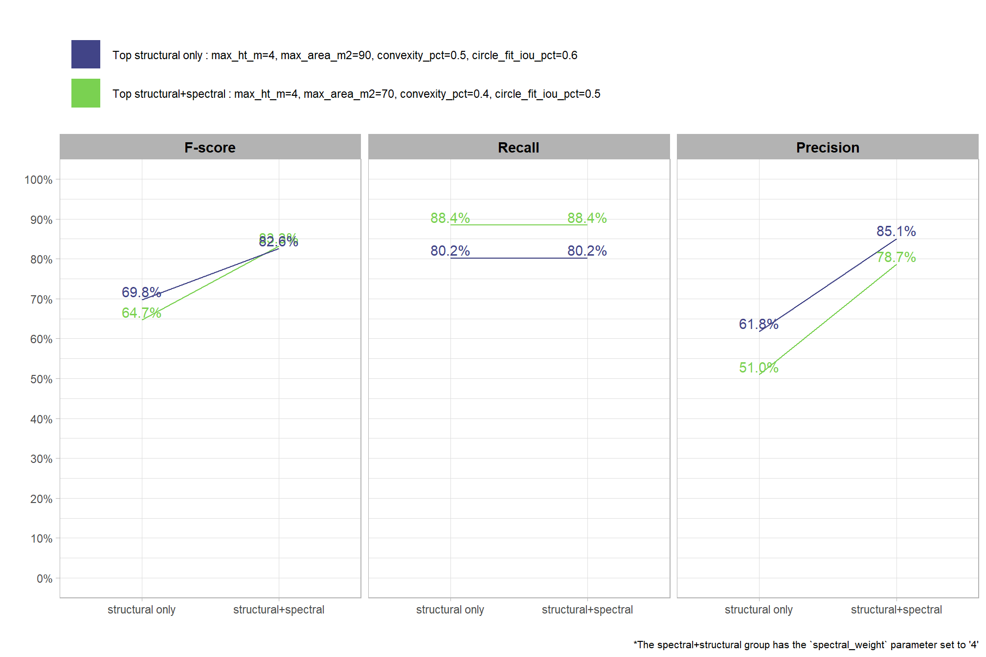
what is the expected MAPE of the top 6 settings by CHM resolution?
# plot it
plt_form_quantification_dist2(
  df = param_combos_ranked %>% dplyr::filter(is_final_selection_chm) %>% dplyr::select(!tidyselect::contains("_pct_rank_"))
  , quant_metric = "mape"
  , paste0(
    "Structural Data Only"
    , "\ndistribution of pile form quantification metrics for the top parameter settings tested"
    , " (n="
    , scales::comma(n_th_top_chm,accuracy=1)
    , ") by CHM resolution"
    , "\nbased on both detection and quantification accuracy"
  )
)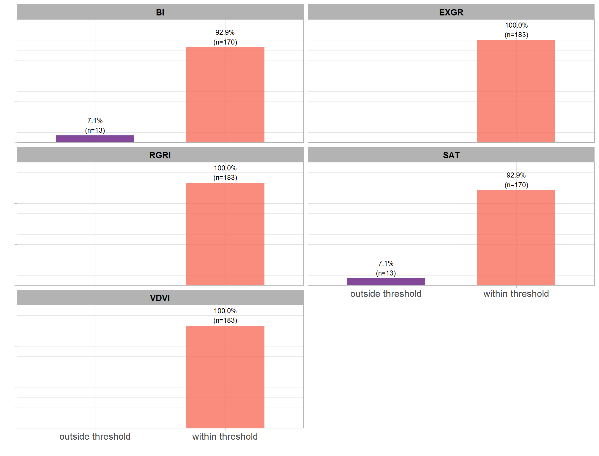
what is the expected Mean Error (ME) of the top 6 settings by CHM resolution?
# plot it
plt_form_quantification_dist2(
  df = param_combos_ranked %>% dplyr::filter(is_final_selection_chm) %>% dplyr::select(!tidyselect::contains("_pct_rank_"))
  , quant_metric = "mean"
  , paste0(
    "Structural Data Only"
    , "\ndistribution of pile form quantification metrics for the top parameter settings tested"
    , " (n="
    , scales::comma(n_th_top_chm,accuracy=1)
    , ") by CHM resolution"
    , "\nbased on both detection and quantification accuracy"
  )
)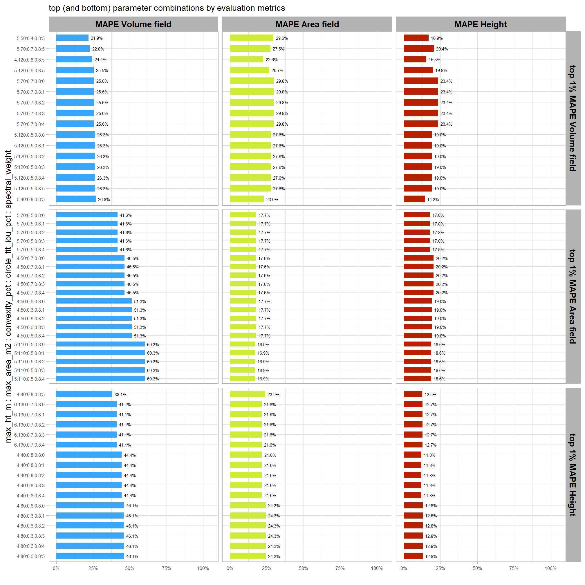
what is the expected RMSE of the top 6 settings by CHM resolution?
# plot it
plt_form_quantification_dist2(
  df = param_combos_ranked %>% dplyr::filter(is_final_selection_chm) %>% dplyr::select(!tidyselect::contains("_pct_rank_"))
  , quant_metric = "rmse"
  , paste0(
    "Structural Data Only"
    , "\ndistribution of pile form quantification metrics for the top parameter settings tested"
    , " (n="
    , scales::comma(n_th_top_chm,accuracy=1)
    , ") by CHM resolution"
    , "\nbased on both detection and quantification accuracy"
  )
)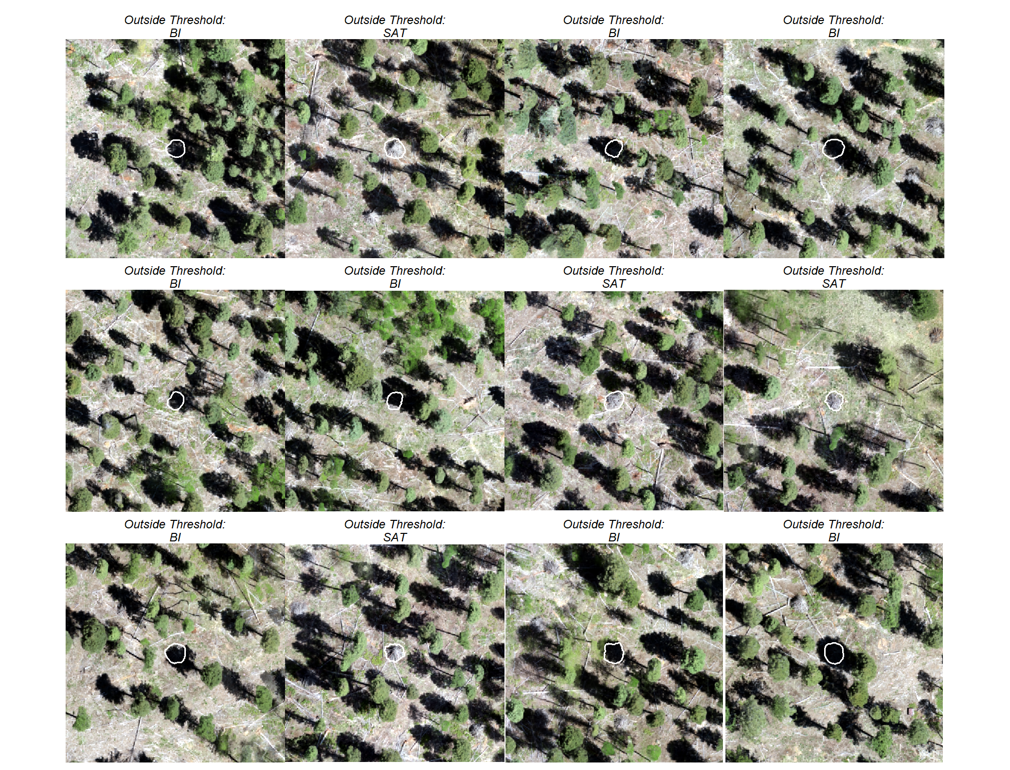
8.6 Data Fusion: Sensitivity Testing
let’s look at the sensitivity testing results for the data fusion approach approach that uses both a CHM generated from aerial point cloud data (for structural information) and RGB imagery
we tested a total of 7,056 combinations per CHM resolution and an overall total of 35,280 combinations
8.6.1 Main Effects: pile detection
what is the detection accuracy across all parameter combinations tested for each CHM resolution?
# plot it
plt_detection_dist2(
  df = param_combos_spectral_gt_agg
  , paste0(
     "Data Fusion"
      , "\ndistribution of pile detection accuracy metrics for all"
     , " (n="
     , scales::comma(n_combos_tested_spectral_chm, accuracy = 1)
     , ") "
     , "parameter combinations tested by CHM resolution"
    )
  , show_rug = F
)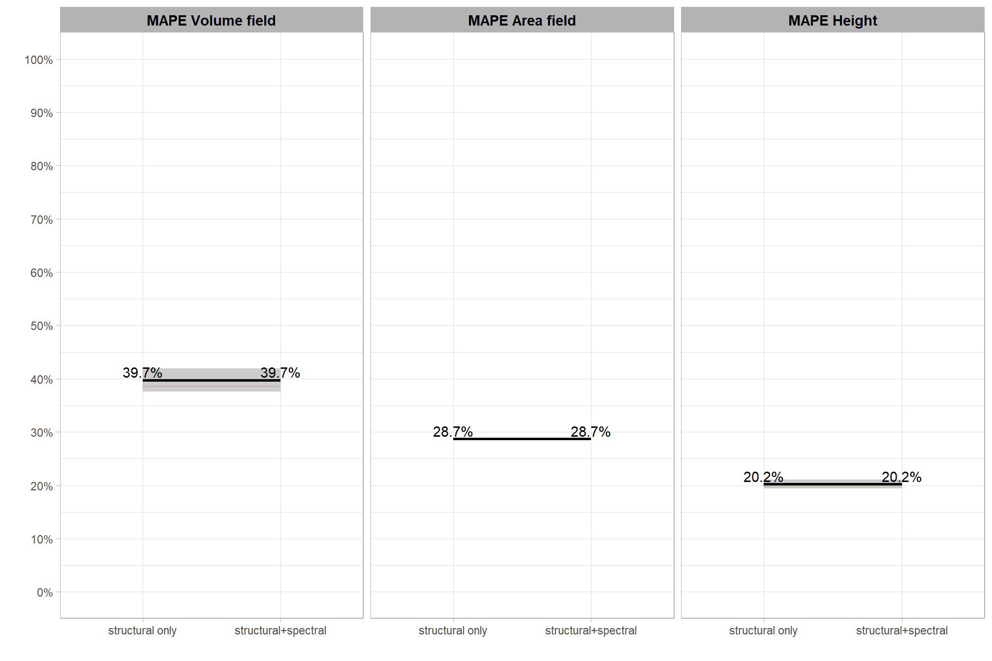
collapsing across all other parameters, what is the main effect of each individual parameter, including the spectral_weight parameter from the data fusion approach, or CHM resolution?
param_combos_spectral_gt_agg %>%
  tidyr::pivot_longer(
    cols = c(precision,recall,f_score)
    , names_to = "metric"
    , values_to = "value"
  ) %>%
  tidyr::pivot_longer(
    cols = c(max_ht_m,max_area_m2,convexity_pct,circle_fit_iou_pct,chm_res_m,spectral_weight)
    , names_to = "param"
    , values_to = "param_value"
  ) %>%
  dplyr::group_by(param, param_value, metric) %>%
  dplyr::summarise(
    median = median(value,na.rm=T)
    , q25 = stats::quantile(value,na.rm=T,probs = 0.25)
    , q75 = stats::quantile(value,na.rm=T,probs = 0.75)
  ) %>%
  dplyr::ungroup() %>%
  dplyr::mutate(
    param = dplyr::case_when(
        param == "spectral_weight" ~ 1
        , param == "chm_res_m" ~ 2
        , param == "max_ht_m" ~ 3
        , param == "min_area_m2" ~ 4
        , param == "max_area_m2" ~ 5
        , param == "convexity_pct" ~ 6
        , param == "circle_fit_iou_pct" ~ 7
      ) %>%
      factor(
        ordered = T
        , levels = 1:7
        , labels = c(
          "spectral_weight"
          , "CHM resolution (m)"
          , "max_ht_m"
          , "min_area_m2"
          , "max_area_m2"
          , "convexity_pct"
          , "circle_fit_iou_pct"
        )
      )
    , metric = dplyr::case_when(
        metric == "f_score" ~ 1
        , metric == "recall" ~ 2
        , metric == "precision" ~ 3
      ) %>%
      factor(
        ordered = T
        , levels = 1:3
        , labels = c(
          "F-score"
          , "Recall"
          , "Precision"
        )
      ) %>%
      forcats::fct_rev()
  ) %>%
  ggplot2::ggplot(
    mapping = ggplot2::aes(y = median, x = param_value, color = metric, fill = metric, group = metric, shape = metric)
  ) +
  ggplot2::geom_ribbon(
    mapping = ggplot2::aes(ymin = q25, ymax = q75)
    , alpha = 0.2, color = NA
  ) +
  ggplot2::geom_line(lwd = 1.5, alpha = 0.8) +
  ggplot2::geom_point(size = 2) +
  ggplot2::facet_wrap(facets = dplyr::vars(param), scales = "free_x") +
  # ggplot2::scale_color_viridis_d(begin = 0.2, end = 0.8) +
  ggplot2::scale_fill_manual(values = rev(pal_eval_metric)) +
  ggplot2::scale_color_manual(values = rev(pal_eval_metric)) +
  ggplot2::scale_y_continuous(limits = c(0,1), labels = scales::percent, breaks = scales::breaks_extended(10)) +
  ggplot2::labs(x = "", y = "median value", color = "", fill = "") +
  ggplot2::theme_light() +
  ggplot2::theme(
    legend.position = "top"
    , strip.text = ggplot2::element_text(size = 11, color = "black", face = "bold")
  ) +
  ggplot2::guides(
    color = ggplot2::guide_legend(override.aes = list(shape = 15, linetype = 0, size = 5, alpha = 1))
    , shape = "none"
  )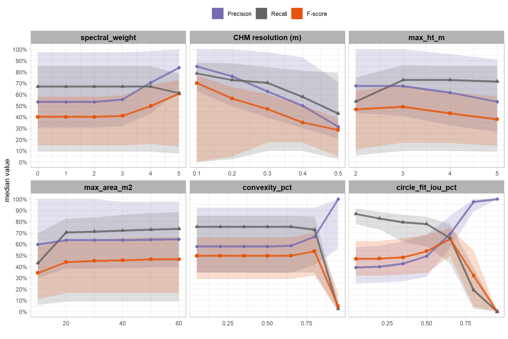
based on these main effect aggregated results, the influence of the parameters specific to the structural detection of slash piles remained the same as when tested without the spectral data. with respect to the spectral_weight parameter included in the data fusion approach:
- increasing the
spectral_weight(where “5” requires all spectral index thresholds to be met) had minimal impact on metrics until a value of “3”, at which point F-score and precision both saw slight improvements. at aspectral_weightof “4”, the F-score significantly improved due to a substantial increase in precision. settingspectral_weightto “5” resulted in a slight drop in recall (detection rate) and a proportionally inverse increase in precision, leading to an additional increase in F-score.
8.6.2 Main Effects: form quantification
let’s check out the the ability of the method to properly extract the form of the piles by looking at the quantification accuracy metrics where:
- Mean Error (ME) represents the direction of bias (over or under-prediction) in the original units
- RMSE represents the typical magnitude of error in the original units, with a stronger penalty for large errors
- MAPE represents the typical magnitude of error as a percentage, allowing for scale-independent comparisons
we expect that the spectral data does not alter the quantification of slash pile form. this is because spectral information is used solely to filter candidate piles, meaning it neither reshapes existing ones nor introduces new detections.
let’s average across all other factors to look at the main effect by parameter for the MAPE metrics quantifying the pile form accuracy
param_combos_spectral_gt_agg %>%
  dplyr::select(
    spectral_weight
    , tidyselect::ends_with("_mape")
  ) %>%
  tidyr::pivot_longer(
    cols = c(tidyselect::ends_with("_mape"))
    , names_to = "metric"
    , values_to = "value"
  ) %>%
  tidyr::pivot_longer(
    cols = c(spectral_weight)
    , names_to = "param"
    , values_to = "param_value"
  ) %>%
  dplyr::group_by(param, param_value, metric) %>%
  dplyr::summarise(
    median = median(value,na.rm=T)
    , q25 = stats::quantile(value,na.rm=T,probs = 0.25)
    , q75 = stats::quantile(value,na.rm=T,probs = 0.75)
  ) %>%
  dplyr::ungroup() %>%
  dplyr::mutate(
    metric = dplyr::case_when(
        metric == "f_score" ~ 1
        , metric == "recall" ~ 2
        , metric == "precision" ~ 3
        # rmse
        , metric == "pct_diff_volume_field_mape" ~ 4
        , metric == "pct_diff_paraboloid_volume_field_mape" ~ 5
        , metric == "pct_diff_area_m2_mape" ~ 6
        , metric == "pct_diff_height_m_mape" ~ 7
        , metric == "pct_diff_diameter_m_mape" ~ 8
      ) %>%
      factor(
        ordered = T
        , levels = 1:8
        , labels = c(
          "F-score"
          , "Recall"
          , "Precision"
          , "MAPE: Volume irregular (%)"
          , "MAPE: Volume paraboloid (%)"
          , "MAPE: Area (%)"
          , "MAPE: Height (%)"
          , "MAPE: Diameter (%)"
        )
      )
    # , param_value = factor(x = param_value, labels = levels(param_combos_spectral_gt$spectral_weight_desc))
  ) %>%
  ggplot2::ggplot(
    mapping = ggplot2::aes(y = median, x = param_value, color = metric, fill = metric, group = metric, shape = metric)
  ) +
  # ggplot2::geom_ribbon(
  #   mapping = ggplot2::aes(ymin = q25, ymax = q75)
  #   , alpha = 0.2, color = NA
  # ) +
  ggplot2::geom_line(lwd = 1.5, alpha = 0.8) +
  ggplot2::geom_point(size = 2) +
  ggplot2::facet_wrap(facets = dplyr::vars(param), scales = "free_x") +
  harrypotter::scale_fill_hp_d(option = "hermionegranger") +
  harrypotter::scale_color_hp_d(option = "hermionegranger") +
  ggplot2::scale_shape_manual(values = c(15,16,17,18,0)) +
  ggplot2::scale_y_continuous(limits = c(0,1), labels = scales::percent, breaks = scales::breaks_extended(10)) +
  ggplot2::labs(x = "", y = "median value", color = "", fill = "") +
  ggplot2::theme_light() +
  ggplot2::theme(
    legend.position = "top"
    , strip.text = ggplot2::element_text(size = 11, color = "black", face = "bold")
  ) +
  ggplot2::guides(
    color = ggplot2::guide_legend(override.aes = list(shape = 15, linetype = 0, size = 5, alpha = 1))
    , shape = "none"
  )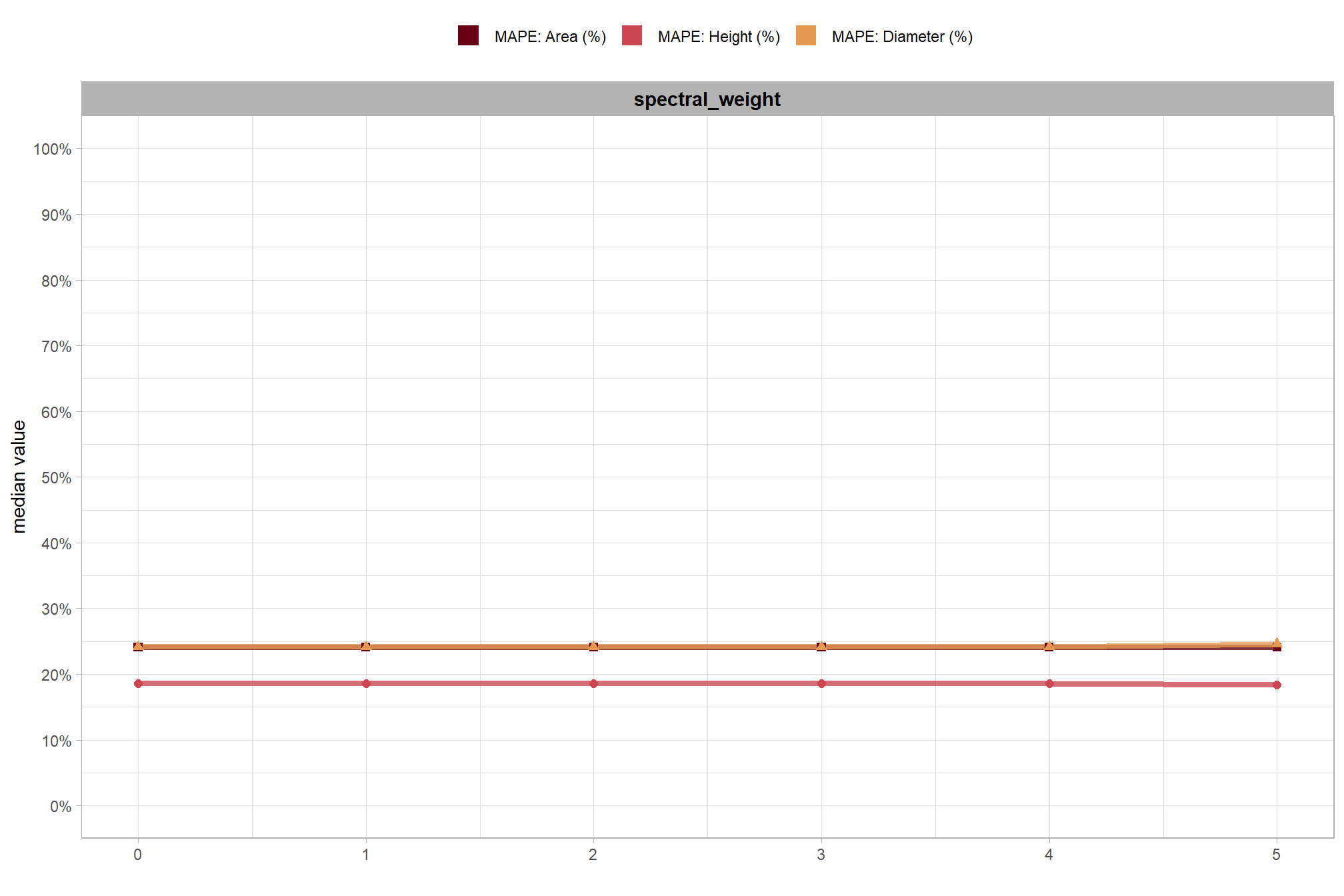
this is exactly what we expected to happen
8.6.3 Top settings
Of those tested, let’s identify the best-performing parameter combinations that not only balance detection and quantification accuracy but also achieve the highest recall rates. we’ll select these by choosing any combination whose recall rate is at least one standard deviation above the average for this top group. if no combinations meet this criterion, we will instead select the top 10 combinations based on their recall rates.
8.6.3.1 Overall (across CHM resolution)
To select the best-performing parameter combinations of those tested, we will prioritize those that balance detection and quantification accuracy. From this group, we will then identify the settings that achieve the highest pile detection rates (recall). We emphasize that these recommendations are for users who can generate a CHM from the original point cloud. This is critical because creating a new CHM at the desired resolution is a fundamentally different process than simply disaggregating an existing, coarser raster.
we’ll use the F-Score and the average rank of the MAPE metrics across all form measurements (i.e. height, diameter, area, volume) to determine the best overall list
# param_combos_spectral_gt_agg %>% nrow()
# param_combos_spectral_gt_agg %>%
#   dplyr::filter(
#     dplyr::if_any(
#       tidyselect::ends_with("_mape")
#       , is.na
#     )
#   ) %>%
#   View()

param_combos_spectral_ranked <-
  param_combos_spectral_gt_agg %>%
  ##########
  # first. find overall top combinations irrespective of CHM res
  ##########
  dplyr::ungroup() %>%
  dplyr::mutate(
    # label combining params
    lab = stringr::str_c(max_ht_m,max_area_m2,convexity_pct,circle_fit_iou_pct,chm_res_m,spectral_weight, sep = ":")
    , dplyr::across(
      .cols = c(tidyselect::ends_with("_mape"))
      , .fn = ~dplyr::percent_rank(-.x)
      , .names = "ovrall_pct_rank_quant_{.col}"
    )
    , dplyr::across(
      .cols = c(f_score)
      # .cols = c(f_score,recall)
      , .fn = ~dplyr::percent_rank(.x)
      , .names = "ovrall_pct_rank_det_{.col}"
    )
  ) %>%
  ##########
  # second. find top combinations by CHM res
  ##########
  dplyr::group_by(chm_res_m) %>%
  dplyr::mutate(
    dplyr::across(
      .cols = c(tidyselect::ends_with("_mape") & !tidyselect::starts_with("ovrall_pct_rank_"))
      , .fn = ~dplyr::percent_rank(-.x)
      , .names = "chm_pct_rank_quant_{.col}"
    )
    , dplyr::across(
      .cols = c(f_score)
      # .cols = c(f_score,recall)
      , .fn = ~dplyr::percent_rank(.x)
      , .names = "chm_pct_rank_det_{.col}"
    )
  ) %>%
  # now get the max of these pct ranks by row
  dplyr::rowwise() %>%
  dplyr::mutate(
    ovrall_pct_rank_quant_mean = mean(
      dplyr::c_across(
        tidyselect::starts_with("ovrall_pct_rank_quant_")
      )
      , na.rm = T
    )
    , ovrall_pct_rank_det_mean = mean(
      dplyr::c_across(
        tidyselect::starts_with("ovrall_pct_rank_det_")
      )
      , na.rm = T
    )
    , chm_pct_rank_quant_mean = mean(
      dplyr::c_across(
        tidyselect::starts_with("chm_pct_rank_quant_")
      )
      , na.rm = T
    )
    , chm_pct_rank_det_mean = mean(
      dplyr::c_across(
        tidyselect::starts_with("chm_pct_rank_det_")
      )
      , na.rm = T
    )
  ) %>%
  dplyr::ungroup() %>%
  # fill na values
  dplyr::mutate(
    dplyr::across(
      .cols = c(ovrall_pct_rank_det_mean, ovrall_pct_rank_quant_mean, chm_pct_rank_det_mean, chm_pct_rank_quant_mean)
      , .fn = ~ifelse(is.na(.x),0,.x)
    )
  ) %>%
  # dplyr::select(ovrall_pct_rank_det_mean, ovrall_pct_rank_quant_mean) %>% summary()
  # now make quadrant var
  dplyr::mutate(
    # groupings for the quadrant plot
    ovrall_accuracy_grp = dplyr::case_when(
        ovrall_pct_rank_det_mean>=0.95 & ovrall_pct_rank_quant_mean>=0.95 ~ 1
        , ovrall_pct_rank_det_mean>=0.90 & ovrall_pct_rank_quant_mean>=0.90 ~ 2
        , ovrall_pct_rank_det_mean>=0.75 & ovrall_pct_rank_quant_mean>=0.75 ~ 3
        , ovrall_pct_rank_det_mean>=0.50 & ovrall_pct_rank_quant_mean>=0.50 ~ 4
        , ovrall_pct_rank_det_mean>=0.50 & ovrall_pct_rank_quant_mean<0.50 ~ 5
        , ovrall_pct_rank_det_mean<0.50 & ovrall_pct_rank_quant_mean>=0.50 ~ 6
        , T ~ 7
      ) %>%
      factor(
        ordered = T
        , levels = 1:7
        , labels = c(
          "top 5% detection & quantification" # ovrall_pct_rank_mean>=0.95 & ovrall_pct_rank_f_score>=0.95 ~ 1
          , "top 10% detection & quantification" # ovrall_pct_rank_mean>=0.90 & ovrall_pct_rank_f_score>=0.90 ~ 2
          , "top 25% detection & quantification" # ovrall_pct_rank_mean>=0.75 & ovrall_pct_rank_f_score>=0.75 ~ 3
          , "top 50% detection & quantification" # ovrall_pct_rank_mean>=0.50 & ovrall_pct_rank_f_score>=0.50 ~ 4
          , "top 50% quantification" # ovrall_pct_rank_mean>=0.50 & ovrall_pct_rank_f_score<0.50 ~ 5
          , "top 50% detection" # ovrall_pct_rank_mean<0.50 & ovrall_pct_rank_f_score>=0.50 ~ 6
          , "bottom 50% detection & quantification"
        )
      )
    , chm_accuracy_grp = dplyr::case_when(
        chm_pct_rank_det_mean>=0.95 & chm_pct_rank_quant_mean>=0.95 ~ 1
        , chm_pct_rank_det_mean>=0.90 & chm_pct_rank_quant_mean>=0.90 ~ 2
        , chm_pct_rank_det_mean>=0.75 & chm_pct_rank_quant_mean>=0.75 ~ 3
        , chm_pct_rank_det_mean>=0.50 & chm_pct_rank_quant_mean>=0.50 ~ 4
        , chm_pct_rank_det_mean>=0.50 & chm_pct_rank_quant_mean<0.50 ~ 5
        , chm_pct_rank_det_mean<0.50 & chm_pct_rank_quant_mean>=0.50 ~ 6
        , T ~ 7
      ) %>%
      factor(
        ordered = T
        , levels = 1:7
        , labels = c(
          "top 5% detection & quantification" # chm_pct_rank_mean>=0.95 & chm_pct_rank_f_score>=0.95 ~ 1
          , "top 10% detection & quantification" # chm_pct_rank_mean>=0.90 & chm_pct_rank_f_score>=0.90 ~ 2
          , "top 25% detection & quantification" # chm_pct_rank_mean>=0.75 & chm_pct_rank_f_score>=0.75 ~ 3
          , "top 50% detection & quantification" # chm_pct_rank_mean>=0.50 & chm_pct_rank_f_score>=0.50 ~ 4
          , "top 50% quantification" # chm_pct_rank_mean>=0.50 & chm_pct_rank_f_score<0.50 ~ 5
          , "top 50% detection" # chm_pct_rank_mean<0.50 & chm_pct_rank_f_score>=0.50 ~ 6
          , "bottom 50% detection & quantification"
        )
      )
    ,
  ) %>%
  ##########
  # first. find overall top combinations irrespective of CHM res
  ##########
  dplyr::ungroup() %>%
  dplyr::mutate(
    ovrall_balanced_pct_rank = dplyr::percent_rank( (ovrall_pct_rank_det_mean+ovrall_pct_rank_quant_mean)/2 ) # equally weight quant and detection
    , ovrall_lab = forcats::fct_reorder(lab, ovrall_balanced_pct_rank)
  ) %>%
  dplyr::arrange(desc(ovrall_balanced_pct_rank),desc(ovrall_pct_rank_det_mean),desc(ovrall_pct_rank_quant_mean)) %>%
  dplyr::mutate(
    ovrall_balanced_rank = dplyr::row_number()
    # is_top_overall = using rows in case not all combos resulted in piles and/or
      # there are many ties in the data leading to no records with a percent rank <= pct_th_top (e.g. many tied at 98%)
    , is_top_overall = dplyr::row_number()<=(n_combos_tested_spectral*pct_th_top)
      # ovrall_balanced_pct_rank>=(1-pct_th_top)
  ) %>%
  dplyr::arrange(desc(is_top_overall),desc(recall),desc(ovrall_pct_rank_det_mean),desc(ovrall_pct_rank_quant_mean),ovrall_balanced_rank) %>%
  dplyr::mutate(is_final_selection = is_top_overall & dplyr::row_number()<=n_th_top) %>%
  ##########
  # second. find top combinations by CHM res
  ##########
  dplyr::group_by(chm_res_m) %>%
  dplyr::mutate(
    chm_balanced_pct_rank = dplyr::percent_rank( (chm_pct_rank_det_mean+chm_pct_rank_quant_mean)/2 ) # equally weight quant and detection
    , chm_lab = forcats::fct_reorder(lab, chm_balanced_pct_rank)
  ) %>%
  dplyr::arrange(chm_res_m,desc(chm_balanced_pct_rank),desc(chm_pct_rank_det_mean),desc(chm_pct_rank_quant_mean),ovrall_balanced_rank) %>%
  dplyr::mutate(
    chm_balanced_rank = dplyr::row_number()
    # is_top_chm = using rows in case not all combos resulted in piles and/or
      # there are many ties in the data leading to no records with a percent rank <= pct_th_top (e.g. many tied at 98%)
    , is_top_chm = dplyr::row_number()<=n_combos_top_spectral_chm # double it so we look at more than 14??
      # chm_balanced_pct_rank>=(1-pct_th_top)
  ) %>%
  dplyr::arrange(chm_res_m,desc(is_top_chm),desc(recall),desc(chm_pct_rank_det_mean),desc(chm_pct_rank_quant_mean),ovrall_balanced_rank) %>%
  dplyr::mutate(is_final_selection_chm = is_top_chm & dplyr::row_number()<=n_th_top_chm) %>% # half it because it's going to be a lot to show in our facet ggplot
  ##### clean up
  dplyr::ungroup() %>%
  dplyr::select(-c(
    c(tidyselect::ends_with("_mape") & tidyselect::starts_with("ovrall_pct_rank_"))
    , c(tidyselect::ends_with("_mape") & tidyselect::starts_with("chm_pct_rank_"))
    , c(tidyselect::ends_with("_f_score") & tidyselect::starts_with("ovrall_pct_rank_"))
    , c(tidyselect::ends_with("_f_score") & tidyselect::starts_with("chm_pct_rank_"))
  ))
# huh?
# param_combos_spectral_ranked %>% dplyr::glimpse()
# param_combos_spectral_ranked %>% dplyr::count(is_final_selection)
to determine the combinations of those tested that achieved the best balance between both detection and quantification accuracy, we’re selecting the parameter combinations that are in the upper-right of the quadrant plot. That is, the parameter combinations that performed best at both pile detection accuracy and pile form quantification accuracy
# plot
param_combos_spectral_ranked %>%
  dplyr::slice_sample(prop = (1/3)) %>%
  ggplot2::ggplot(
    mapping=ggplot2::aes(x = ovrall_pct_rank_det_mean, y = ovrall_pct_rank_quant_mean, color = ovrall_accuracy_grp)
  ) +
  ggplot2::geom_vline(xintercept = 0.5, color = "gray22") +
  ggplot2::geom_hline(yintercept = 0.5, color = "gray22") +
  ggplot2::geom_vline(xintercept = 0.75, color = "gray44") +
  ggplot2::geom_hline(yintercept = 0.75, color = "gray44") +
  ggplot2::geom_vline(xintercept = 0.9, color = "gray66") +
  ggplot2::geom_hline(yintercept = 0.9, color = "gray66") +
  ggplot2::geom_point() +
  ggplot2::scale_colour_viridis_d(direction = -1) +
  ggplot2::scale_x_continuous(
    labels = scales::percent_format(accuracy = 1)
    , limits = c(0,1)
  ) +
  ggplot2::scale_y_continuous(
    labels = scales::percent_format(accuracy = 1)
    , limits = c(0,1)
  ) +
  ggplot2::labs(
    x = "Percentile F-Score", y = "Percentile MAPE (mean)"
    , color = ""
    , subtitle = "Data Fusion"
  ) +
  ggplot2::theme_light() +
  ggplot2::theme(
    legend.position = "bottom"
    , legend.text = ggplot2::element_text(size = 8)
    , strip.text = ggplot2::element_text(size = 11, color = "black", face = "bold")
    , axis.text = ggplot2::element_text(size = 7)
  ) +
  ggplot2::guides(
    color = ggplot2::guide_legend(override.aes = list(shape = 15, linetype = 0, size = 5, alpha = 1))
    , shape = "none"
  )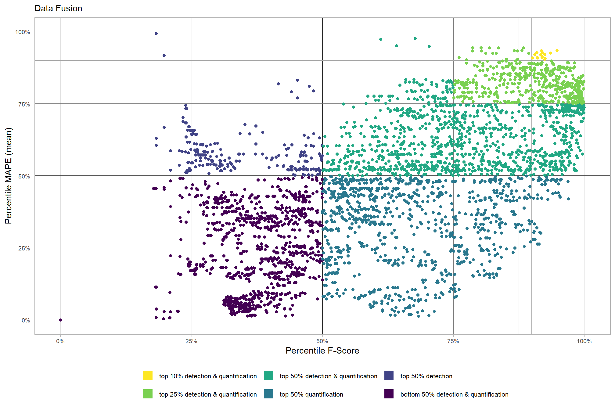
8.6.3.1.1 Top 1.0%
let’s check out the parameter settings of the top 1.0% (n=352) from all 35,280 combinations tested. these are “votes” for the parameter setting based on the combinations that achieved the best balance between both detection and quantification accuracy.
param_combos_spectral_ranked %>%
  dplyr::filter(is_top_overall) %>%
  dplyr::select(tidyselect::contains("f_score"), max_ht_m,max_area_m2,convexity_pct,circle_fit_iou_pct,chm_res_m,spectral_weight) %>%
  tidyr::pivot_longer(
    cols = c(max_ht_m,max_area_m2,convexity_pct,circle_fit_iou_pct,chm_res_m,spectral_weight)
    , names_to = "metric"
    , values_to = "value"
  ) %>%
  dplyr::count(metric, value) %>%
  dplyr::group_by(metric) %>%
  dplyr::mutate(
    pct=n/sum(n)
    , lab = paste0(scales::percent(pct,accuracy=0.1), "\nn=", scales::comma(n,accuracy=1))
  ) %>%
  ggplot2::ggplot(
    mapping = ggplot2::aes(x = factor(value), y=pct, label=lab, fill = metric)
  ) +
  ggplot2::geom_col(width = 0.6) +
  ggplot2::geom_text(color = "black", size = 2.5, vjust = -0.2) +
  ggplot2::facet_wrap(facets = dplyr::vars(metric), ncol=2, scales = "free_x") +
  ggplot2::scale_y_continuous(
    breaks = seq(0,1,by=0.2)
    , labels = scales::percent
    , expand = ggplot2::expansion(mult = c(0,0.2))
  ) +
  ggplot2::scale_fill_manual(values = pal_param[1:6]) +
  ggplot2::labs(
    x = "parameter setting", y = ""
    , fill = ""
    , subtitle = paste0(
      "Data Fusion"
       , "\nparameter settings of top "
       , scales::percent(pct_th_top,accuracy=0.1)
       , " (n="
       , scales::comma(sum(param_combos_spectral_ranked$is_top_overall), accuracy = 1)
       , ") "
       , "overall parameter combinations\nbased on both detection and quantification accuracy"
    )
  ) +
  ggplot2::theme_light() +
  ggplot2::theme(
    legend.position = "none"
    , strip.text = ggplot2::element_text(size = 11, color = "black", face = "bold")
    , axis.text.y = ggplot2::element_text(size = 6)
    , axis.text.x = ggplot2::element_text(size = 8)
    , plot.subtitle = ggplot2::element_text(size = 8)
  )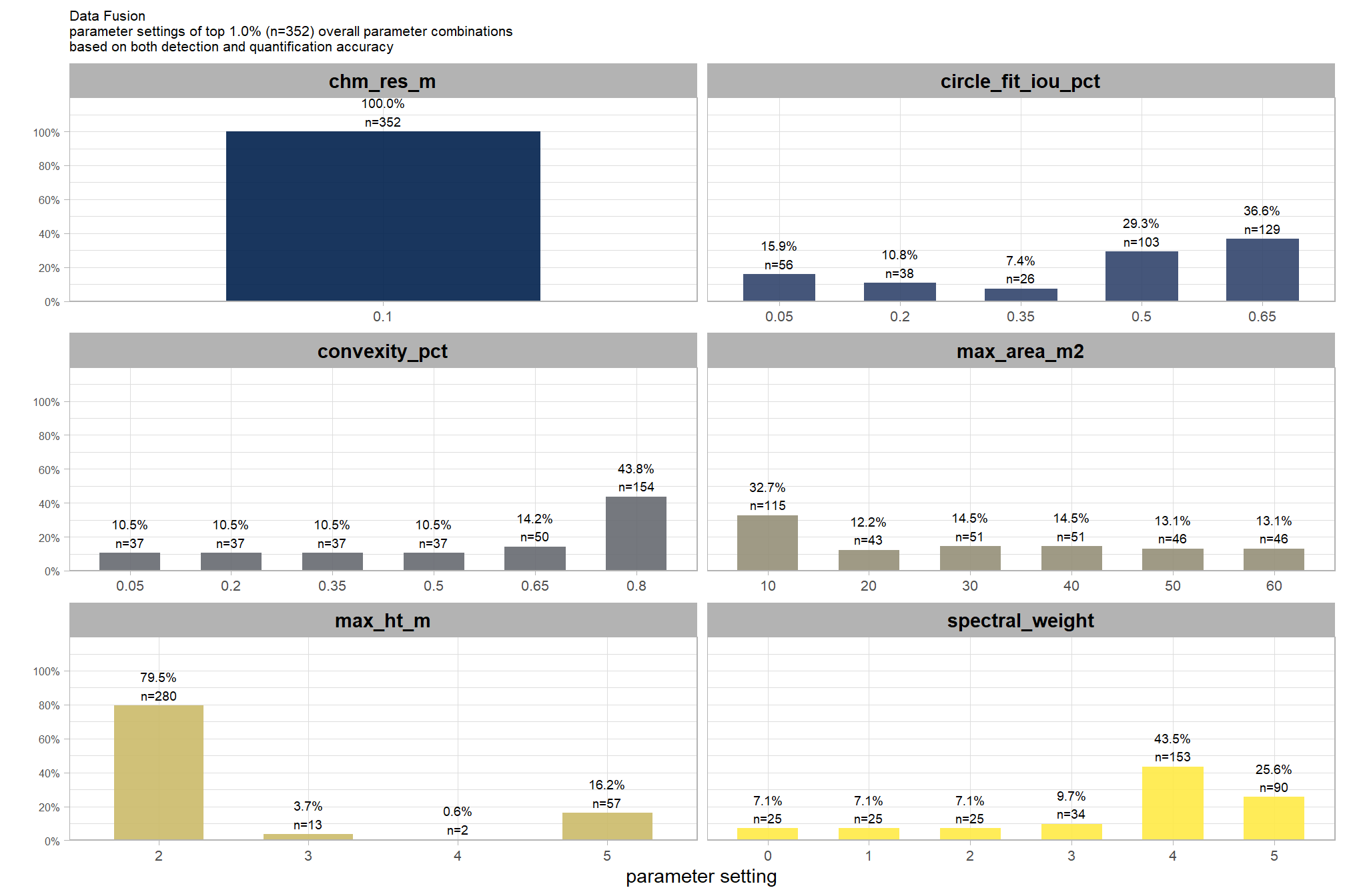
what is the expected detection accuracy of the top 1.0% (n=352) combinations tested?
plt_detection_dist(
  df = param_combos_spectral_ranked %>% dplyr::filter(is_top_overall) %>% dplyr::select(!tidyselect::contains("_pct_rank_"))
  , paste0(
    "Data Fusion"
    , "\ndistribution of pile detection metrics for top "
    , scales::percent(pct_th_top,accuracy=0.1)
    , " (n="
    , scales::comma(sum(param_combos_spectral_ranked$is_top_overall), accuracy = 1)
    , ") "
    , "overall parameter combinations\nbased on both detection and quantification accuracy"
  )
)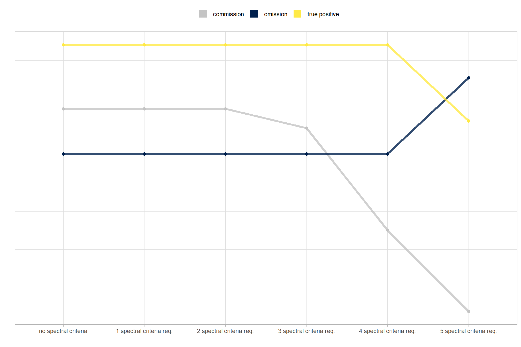
what is the expected quantification accuracy of the top 1.0% (n=352) combinations tested?
# plot it
plt_form_quantification_dist(
  df = param_combos_spectral_ranked %>% dplyr::filter(is_top_overall) %>% dplyr::select(!tidyselect::contains("_pct_rank_"))
  , paste0(
    "Structural Data Only"
    , "\ndistribution of pile form quantification metrics for the top "
    , scales::percent(pct_th_top,accuracy=0.1)
    , " (n="
    , scales::comma(sum(param_combos_spectral_ranked$is_top_overall), accuracy = 1)
    , ") "
    , "overall parameter combinations\nbased on both detection and quantification accuracy"
  )
)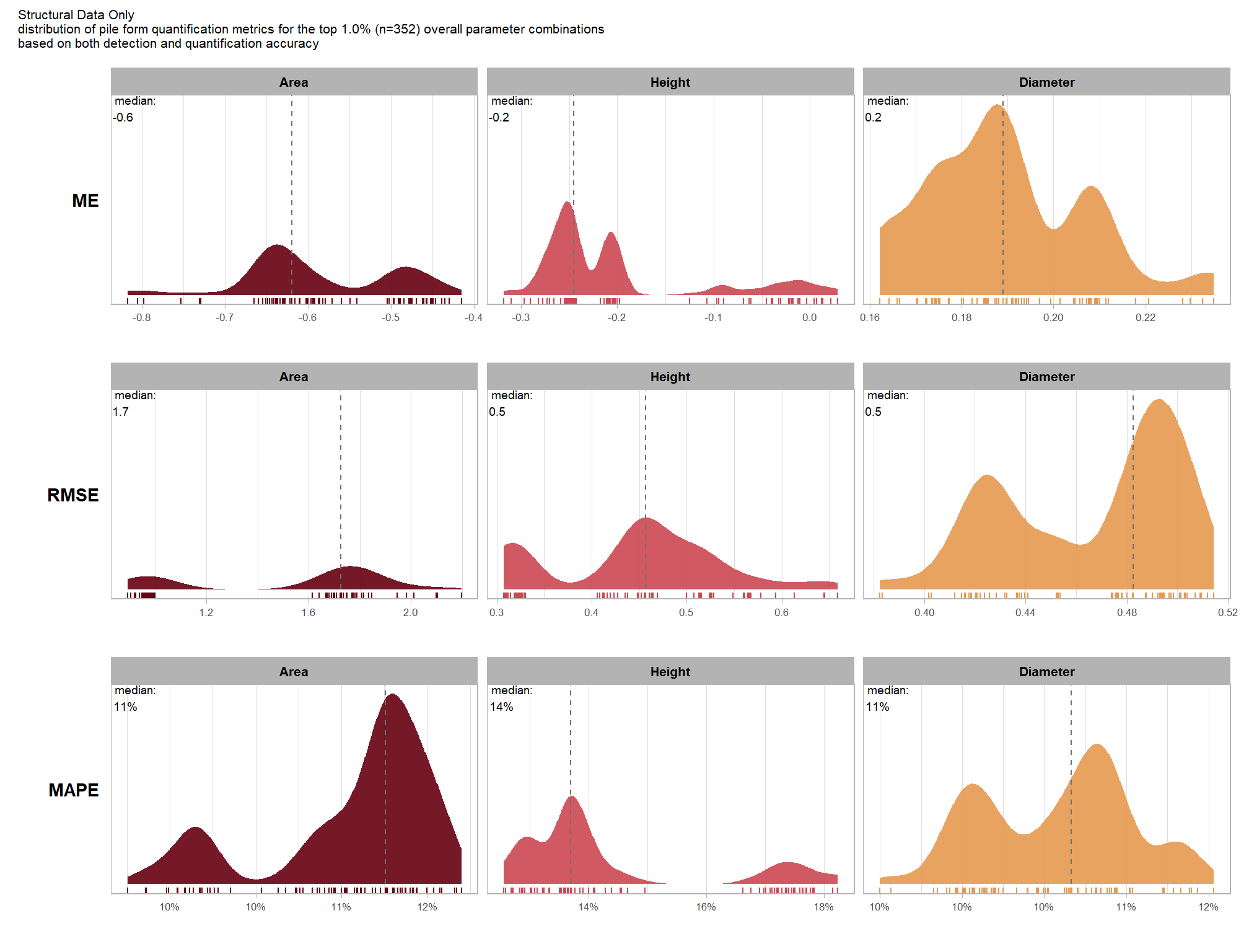
8.6.3.1.2 Top 12 settings
Let’s focus on the top 12 parameter settings tested to highlight the pile detection and form quantification accuracies achieved by these settings
# pal_temp %>% scales::show_col()
# filter and reshape
param_combos_spectral_ranked %>%
  dplyr::filter(is_final_selection) %>%
  dplyr::select(!tidyselect::contains("_pct_rank_")) %>%
  dplyr::select(
    max_ht_m,max_area_m2,convexity_pct,circle_fit_iou_pct,chm_res_m,spectral_weight
    , ovrall_lab
    # detection
    , f_score, recall, precision
    # quantification
    , tidyselect::ends_with("_rmse")
    , tidyselect::ends_with("_rrmse")
    , tidyselect::ends_with("_mean")
    , tidyselect::ends_with("_mape")
  ) %>%
  tidyr::pivot_longer(
    cols = c(
      f_score, recall, precision
      , tidyselect::ends_with("_rmse")
      , tidyselect::ends_with("_rrmse")
      , tidyselect::ends_with("_mean")
      , tidyselect::ends_with("_mape")
    )
    , names_to = "metric"
    , values_to = "value"
  ) %>%
  dplyr::mutate(
    eval_metric = stringr::str_extract(metric, "(_rmse|_rrmse|_mean|_mape|f_score|recall|precision)$") %>%
      stringr::str_remove_all("_") %>%
      stringr::str_replace_all("mean","me") %>%
      toupper() %>%
      factor(
        ordered = T
        , levels = c("FSCORE","RECALL","PRECISION", "ME","RMSE","RRMSE","MAPE")
        , labels = c("F-score","Recall","Precision", "ME","RMSE","RRMSE","MAPE")
      )
    , pile_metric = metric %>%
      stringr::str_remove("(_rmse|_rrmse|_mean|_mape)$") %>%
      stringr::str_extract("(paraboloid_volume|volume|area|height|diameter)") %>%
      dplyr::coalesce("detection") %>%
      factor(
        ordered = T
        , levels = c(
          "detection"
          , "volume"
          , "paraboloid_volume"
          , "area"
          , "height"
          , "diameter"
        )
        , labels = c(
          "Detection"
          , "Volume"
          , "Volume paraboloid"
          , "Area (m2)"
          , "Height (m)"
          , "Diameter (m)"
        )
      )
    , value_lab = dplyr::case_when(
        eval_metric %in% c("F-score","Recall","Precision", "RRMSE", "MAPE") ~ scales::percent(value,accuracy=0.1)
        , eval_metric == "ME" ~ scales::comma(value,accuracy=0.01)
        , T ~ scales::comma(value,accuracy=0.1)
      )
  ) %>%
  # make var for color
  dplyr::group_by(pile_metric, eval_metric) %>%
  dplyr::mutate(
    # for ME, color by abs...for f-score,recall,precision color by -value so that higher means better...
      # ...since higher means worse for quantification accuracy metrics
    value_dir = dplyr::case_when(
      eval_metric %in% c("ME") ~ abs(value)
      , eval_metric %in% c("F-score","Recall","Precision") ~ -value
      , T ~ value
    )
    , value_z = (value_dir-mean(value_dir,na.rm=T))/sd(value_dir,na.rm=T) # this is the key to the different colors within facets
  ) %>%
  dplyr::ungroup() %>%
  dplyr::filter(!eval_metric %in% c("RRMSE")) %>%
  # View()
  ggplot2::ggplot(mapping = ggplot2::aes(x = eval_metric, y = ovrall_lab)) +
  ggplot2::geom_tile(
    mapping = ggplot2::aes(fill = pile_metric, alpha = -value_z)
    , color = "gray"
  ) +
  ggplot2::geom_text(
    mapping = ggplot2::aes(label = value_lab, fontface = "bold")
    , color = "white"
  ) +
  ggplot2::facet_grid(cols = dplyr::vars(pile_metric), scales = "free_x") +
  ggplot2::scale_x_discrete(position = "top") +
  ggplot2::scale_fill_manual(values = c("gray33", harrypotter::hp(n=3,option = "hermionegranger") )) +
  ggplot2::scale_alpha_binned(range = c(0.55, 1)) + # this is the key to the different colors within facets
  ggplot2::theme_light() +
  ggplot2::labs(
    x = ""
    , y = "max_ht_m : max_area_m2 : convexity_pct : circle_fit_iou_pct : chm_res_m : spectral_weight"
    , subtitle = paste0(
       "Data Fusion"
       , "\npile detection and form quantification accuracy metrics for the top parameter settings tested"
       # , scales::percent(1-pct_rank_th_top,accuracy=1)
       , " (n="
       , scales::comma(n_th_top,accuracy=1)
       , ") "
       , "\nbased on both detection and quantification accuracy"
      )
    , caption = "*darker colors indicate relatively higher accuracy values"
  ) +
  ggplot2::theme(
    legend.position = "none"
    , panel.grid = ggplot2::element_blank()
    , strip.placement = "outside"
    , strip.text.x = ggplot2::element_text(size = 8, color = "black", face = "bold")
    , axis.text.x = ggplot2::element_text(size = 7, color = "black", face = "bold")
    , axis.title.x = ggplot2::element_blank()
    , plot.subtitle = ggplot2::element_text(size = 8)
  )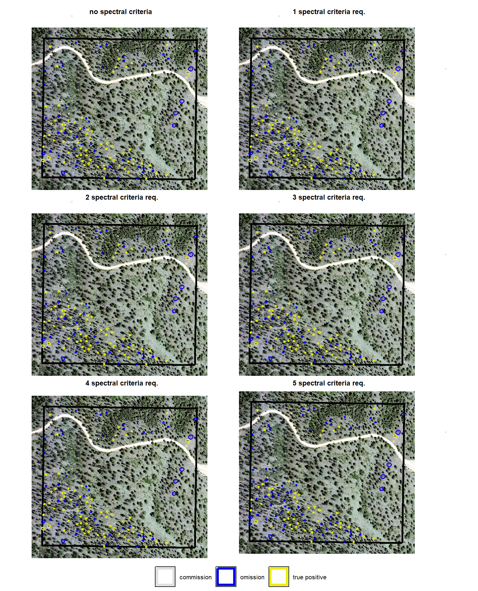
this plot allows for a simultaneous comparison of all metrics for pile detection and pile form quantification. it includes only the parameter combinations that achieved the best balanced accuracy, helping users identify the optimal settings by evaluating the trade-offs between detection and form quantification.
let’s table this
param_combos_spectral_ranked %>%
  dplyr::filter(is_final_selection) %>%
  dplyr::select(!tidyselect::contains("_pct_rank_")) %>%
  # first select to arrange eval_metric
  dplyr::select(
    ovrall_lab
    , max_ht_m,max_area_m2,convexity_pct,circle_fit_iou_pct,chm_res_m,spectral_weight
    # detection
    , f_score, recall, precision
    # quantification
    , tidyselect::ends_with("_mean")
    , tidyselect::ends_with("_rmse")
    # , tidyselect::ends_with("_rrmse")
    , tidyselect::ends_with("_mape")
  ) %>%
  # second select to arrange pile_metric
  dplyr::select(
    ovrall_lab
    , max_ht_m,max_area_m2,convexity_pct,circle_fit_iou_pct,chm_res_m,spectral_weight
    # detection
    , f_score, recall, precision
    # quantification
    , c(tidyselect::contains("volume") & !tidyselect::contains("paraboloid"))
    , tidyselect::contains("area")
    , tidyselect::contains("height")
    , tidyselect::contains("diameter")
  ) %>%
  # names()
  dplyr::mutate(
    dplyr::across(
      .cols = c(f_score, recall, precision, tidyselect::ends_with("_mape"))
      , .fn = ~ scales::percent(.x, accuracy = 1)
    )
    , dplyr::across(
      .cols = c(tidyselect::ends_with("_mean"))
      , .fn = ~ scales::comma(.x, accuracy = 0.01)
    )
    , dplyr::across(
      .cols = c(tidyselect::ends_with("_rmse"))
      , .fn = ~ scales::comma(.x, accuracy = 0.1)
    )
  ) %>%
  dplyr::mutate(blank= "   " ) %>%
  dplyr::relocate(blank, .before = f_score) %>%
  dplyr::arrange(desc(ovrall_lab)) %>%
  kableExtra::kbl(
    caption =
      paste0(
       "Data Fusion"
       , "<br>pile detection and form quantification accuracy metrics for the top parameter settings tested"
       # , scales::percent(1-pct_rank_th_top,accuracy=1)
       , " (n="
       , scales::comma(n_th_top,accuracy=1)
       , ") "
       , "<br>based on both detection and quantification accuracy"
      )
    , col.names = c(
      ""
      ,"max_ht_m","max_area_m2","convexity_pct","circle_fit_iou_pct","chm_res_m","spectral_weight"
      , "   "
      , "F-score", "Recall", "Precision"
      , rep(c("ME","RMSE","MAPE"), times = 3)
    )
    , escape = F
  ) %>%
  kableExtra::kable_styling(font_size = 11) %>%
  kableExtra::add_header_above(c(
    " "=8
    , "Detection" = 3
    # , "Volume" = 3
    , "Area" = 3
    , "Height" = 3
    , "Diameter" = 3
  )) %>%
  kableExtra::column_spec(seq(8,20,by=3), border_right = TRUE, include_thead = TRUE) %>%
  kableExtra::column_spec(
    column = 8:20
    , extra_css = "font-size: 10px;"
    , include_thead = T
  ) %>%
kableExtra::scroll_box(width = "740px") | max_ht_m | max_area_m2 | convexity_pct | circle_fit_iou_pct | chm_res_m | spectral_weight | F-score | Recall | Precision | ME | RMSE | MAPE | ME | RMSE | MAPE | ME | RMSE | MAPE | ||
|---|---|---|---|---|---|---|---|---|---|---|---|---|---|---|---|---|---|---|---|
| 5:60:0.8:0.65:0.1:4 | 5 | 60 | 0.80 | 0.65 | 0.1 | 4 | 89% | 90% | 88% | -0.80 | 2.1 | 10% | -0.10 | 0.6 | 18% | 0.21 | 0.5 | 10% | |
| 5:50:0.8:0.65:0.1:4 | 5 | 50 | 0.80 | 0.65 | 0.1 | 4 | 89% | 90% | 88% | -0.80 | 2.1 | 10% | -0.10 | 0.6 | 18% | 0.21 | 0.5 | 10% | |
| 5:60:0.65:0.65:0.1:4 | 5 | 60 | 0.65 | 0.65 | 0.1 | 4 | 89% | 91% | 87% | -0.81 | 2.1 | 10% | -0.09 | 0.6 | 18% | 0.21 | 0.5 | 10% | |
| 5:60:0.5:0.65:0.1:4 | 5 | 60 | 0.50 | 0.65 | 0.1 | 4 | 89% | 91% | 87% | -0.81 | 2.1 | 10% | -0.09 | 0.6 | 18% | 0.21 | 0.5 | 10% | |
| 5:60:0.35:0.65:0.1:4 | 5 | 60 | 0.35 | 0.65 | 0.1 | 4 | 89% | 91% | 87% | -0.81 | 2.1 | 10% | -0.09 | 0.6 | 18% | 0.21 | 0.5 | 10% | |
| 5:60:0.2:0.65:0.1:4 | 5 | 60 | 0.20 | 0.65 | 0.1 | 4 | 89% | 91% | 87% | -0.81 | 2.1 | 10% | -0.09 | 0.6 | 18% | 0.21 | 0.5 | 10% | |
| 5:60:0.05:0.65:0.1:4 | 5 | 60 | 0.05 | 0.65 | 0.1 | 4 | 89% | 91% | 87% | -0.81 | 2.1 | 10% | -0.09 | 0.6 | 18% | 0.21 | 0.5 | 10% | |
| 5:50:0.65:0.65:0.1:4 | 5 | 50 | 0.65 | 0.65 | 0.1 | 4 | 89% | 91% | 87% | -0.81 | 2.1 | 10% | -0.09 | 0.6 | 18% | 0.21 | 0.5 | 10% | |
| 5:50:0.5:0.65:0.1:4 | 5 | 50 | 0.50 | 0.65 | 0.1 | 4 | 89% | 91% | 87% | -0.81 | 2.1 | 10% | -0.09 | 0.6 | 18% | 0.21 | 0.5 | 10% | |
| 5:50:0.35:0.65:0.1:4 | 5 | 50 | 0.35 | 0.65 | 0.1 | 4 | 89% | 91% | 87% | -0.81 | 2.1 | 10% | -0.09 | 0.6 | 18% | 0.21 | 0.5 | 10% | |
| 5:50:0.2:0.65:0.1:4 | 5 | 50 | 0.20 | 0.65 | 0.1 | 4 | 89% | 91% | 87% | -0.81 | 2.1 | 10% | -0.09 | 0.6 | 18% | 0.21 | 0.5 | 10% | |
| 5:50:0.05:0.65:0.1:4 | 5 | 50 | 0.05 | 0.65 | 0.1 | 4 | 89% | 91% | 87% | -0.81 | 2.1 | 10% | -0.09 | 0.6 | 18% | 0.21 | 0.5 | 10% |
what is the expected detection accuracy of the top 12 settings?
plt_detection_dist(
  df = param_combos_spectral_ranked %>% dplyr::filter(is_final_selection) %>% dplyr::select(!tidyselect::contains("_pct_rank_"))
  , paste0(
    "Data Fusion"
    , "\ndistribution of pile detection metrics for the top parameter settings tested"
    , " (n="
    , scales::comma(n_th_top,accuracy=1)
    , ") "
    , "\nbased on both detection and quantification accuracy"
  )
)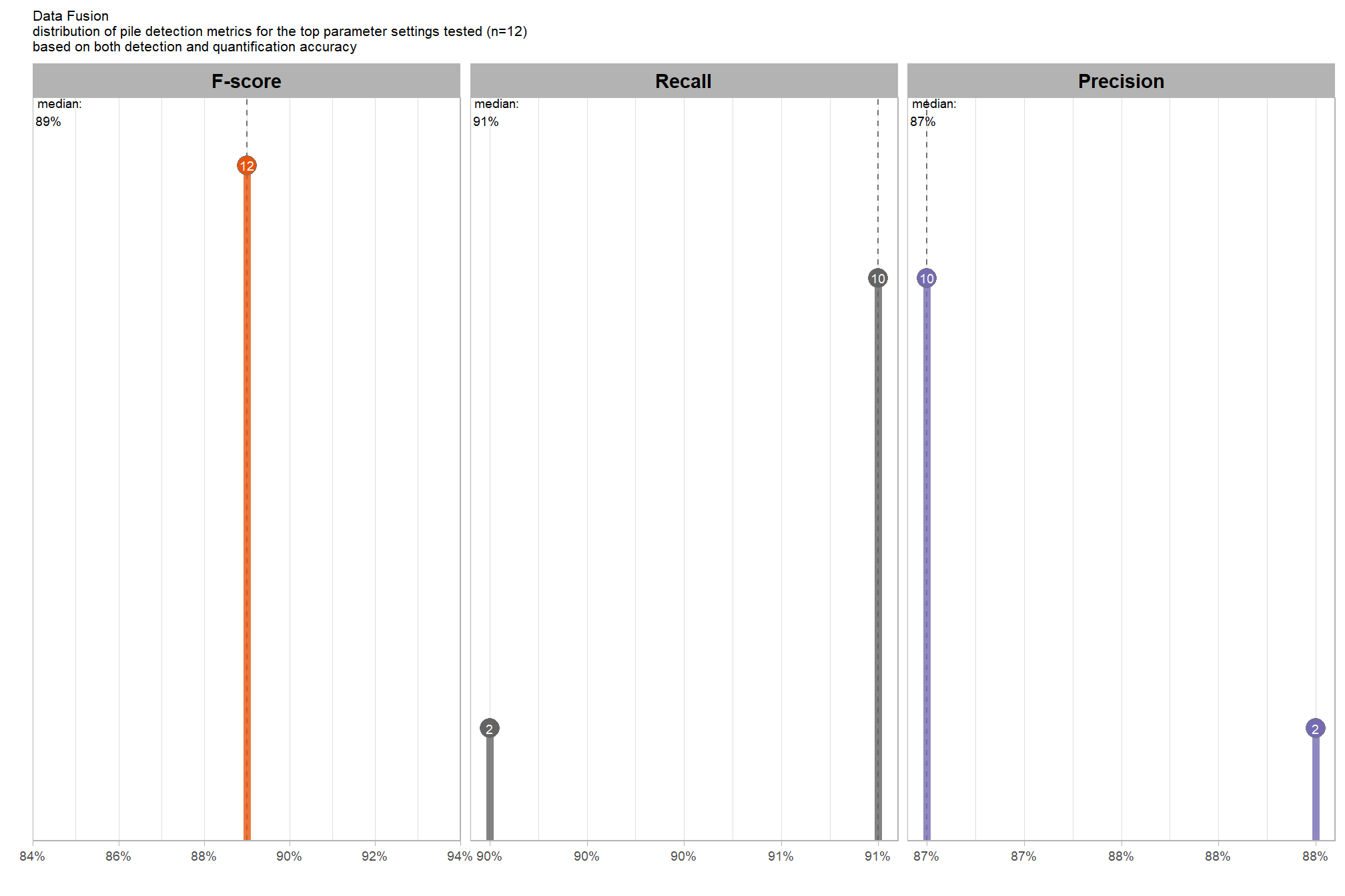
what is the expected quantification accuracy of the top 12 settings?
# plot it
plt_form_quantification_dist(
  df = param_combos_spectral_ranked %>% dplyr::filter(is_final_selection) %>% dplyr::select(!tidyselect::contains("_pct_rank_"))
  , paste0(
    "Data Fusion"
    , "\ndistribution of pile form quantification metrics for the top parameter settings tested"
    , " (n="
    , scales::comma(n_th_top,accuracy=1)
    , ") "
    , "\nbased on both detection and quantification accuracy"
  )
)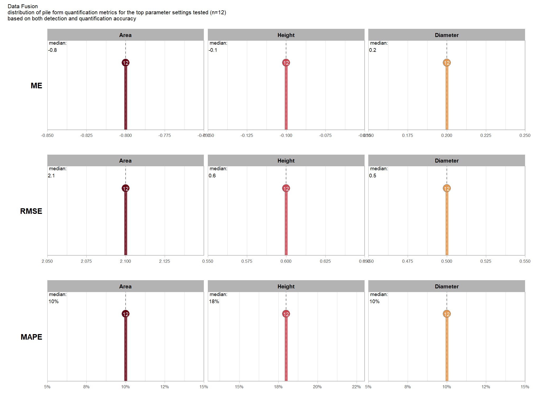
finally, here are the combinations selected compared against all 35,280 combinations tested.
dplyr::bind_rows(
  param_combos_spectral_ranked %>% dplyr::filter(is_final_selection)
  , param_combos_spectral_ranked %>% dplyr::filter(!is_final_selection) %>% dplyr::slice_sample(prop = (1/6))
) %>%
  dplyr::select(
    rn,max_ht_m,max_area_m2,convexity_pct,circle_fit_iou_pct
    , is_final_selection
    , f_score, precision, recall
    # quantification accuracy
    , tidyselect::ends_with("_mape")
  ) %>%
  tidyr::pivot_longer(
    cols = c(
      tidyselect::ends_with("_mape")
      # ,precision,recall
    )
    , names_to = "metric"
    , values_to = "value"
  ) %>%
  dplyr::mutate(
    eval_metric = stringr::str_extract(metric, "(_rmse|_rrmse|_mean|_mape)$") %>%
      stringr::str_remove_all("_") %>%
      stringr::str_replace_all("mean","me") %>%
      toupper() %>%
      factor(
        ordered = T
        , levels = c("ME","RMSE","RRMSE","MAPE")
      )
    , pile_metric = metric %>%
      stringr::str_remove("(_rmse|_rrmse|_mean|_mape)$") %>%
      stringr::str_extract("(paraboloid_volume|volume|area|height|diameter|precision|recall)") %>%
      factor(
        ordered = T
        , levels = c(
          "volume"
          , "paraboloid_volume"
          , "area"
          , "height"
          , "diameter"
          , "recall"
          , "precision"
        )
        , labels = c(
          "Volume"
          , "Volume paraboloid"
          , "Area (m2)"
          , "Height (m)"
          , "Diameter (m)"
          , "Recall"
          , "Precision"
        )
      )
    , color_metric = ifelse(is_final_selection, pile_metric, NA) %>% factor()
  ) %>%
  dplyr::arrange(is_final_selection) %>%
  # plot
  ggplot2::ggplot(mapping = ggplot2::aes(x = f_score, y = value, color = color_metric)) +
  ggplot2::geom_point() +
  ggplot2::facet_wrap(facets = dplyr::vars(pile_metric)) +
  harrypotter::scale_color_hp_d(option = "hermionegranger", na.value = "gray88") +
  ggplot2::scale_x_continuous(
    labels = scales::percent_format(accuracy = 1)
    , limits = c(0,1)
  ) +
  ggplot2::scale_y_continuous(
    labels = scales::percent_format(accuracy = 1)
    , limits = c(0,NA)
  ) +
  ggplot2::labs(x = "F-Score", y = "MAPE", caption = "*records in gray not selected") +
  ggplot2::theme_light() +
  ggplot2::theme(
    legend.position = "none"
    , strip.text = ggplot2::element_text(size = 11, color = "black", face = "bold")
  )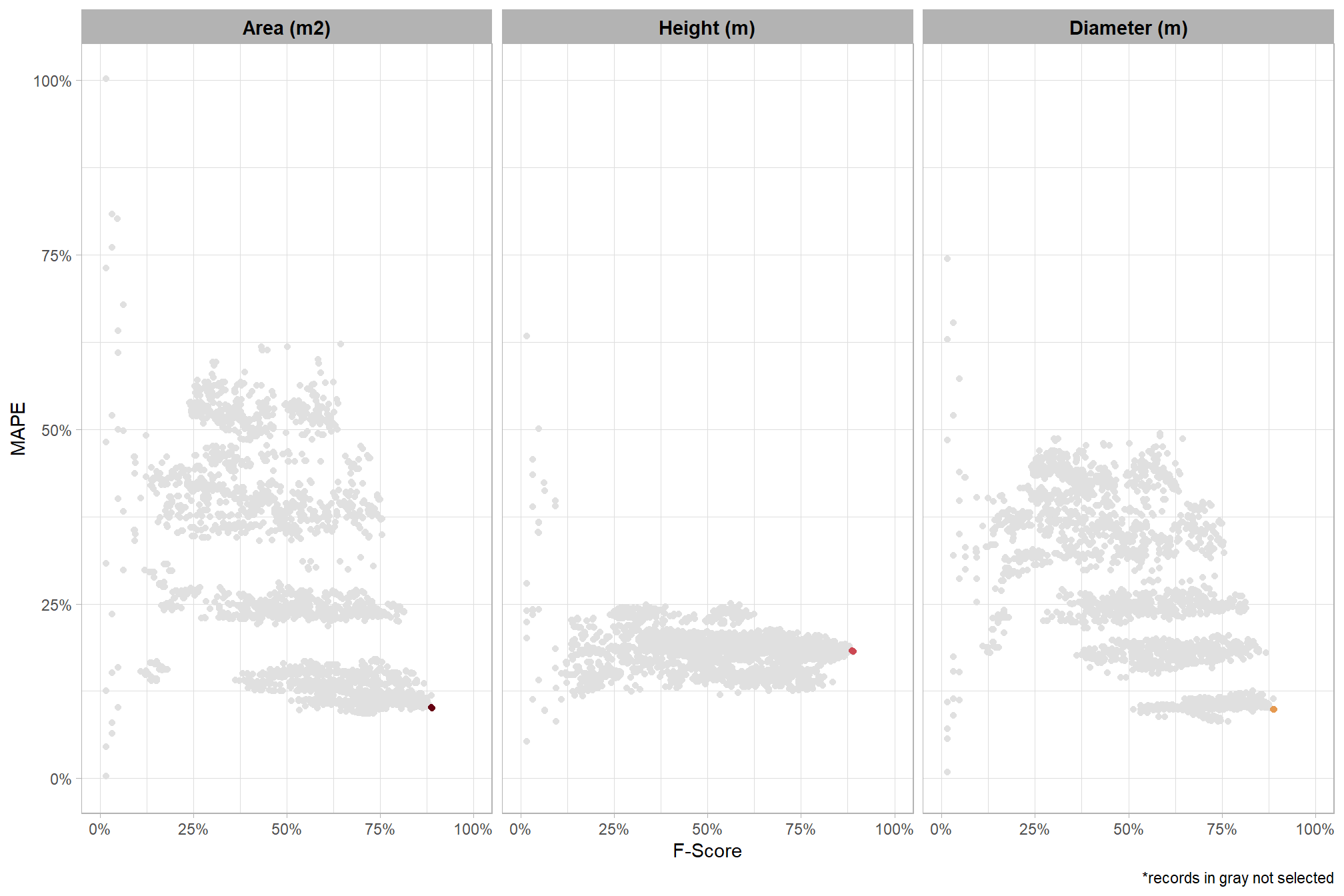
8.6.3.2 by CHM resolution
To select the best-performing parameter combinations of those tested by CHM resolution, we will prioritize those that balance detection and quantification accuracy. From this group, we will then identify the settings that achieve the highest pile detection rates (recall). These recommendations are for users who are working with a CHM with a resolution in the range of those tested for this analysis or can aggregate (i.e. make more coarse) a CHM to a resolution tested for the purpose of either improving processing performance or enhancing pile detection and/or quantification accuracy based on the results shown here
we already created this data above (param_combos_ranked) using the F-Score and the average rank of the MAPE metrics across all form measurements (i.e. height, diameter, area, volume) to determine the best overall list of those tested by CHM resolution
8.6.3.2.1 Top 2.0%
Of those tested, let’s check out the parameter settings of the top 2.0% (n=141) from all 7,056 combinations tested by CHM resolution. these are “votes” for the parameter setting based on the combinations that achieved the best balance between both detection and quantification accuracy.
param_combos_spectral_ranked %>%
  dplyr::filter(is_top_chm) %>%
  dplyr::select(tidyselect::contains("f_score"), max_ht_m,max_area_m2,convexity_pct,circle_fit_iou_pct,chm_res_m,chm_res_m_desc,spectral_weight) %>%
  tidyr::pivot_longer(
    cols = c(max_ht_m,max_area_m2,convexity_pct,circle_fit_iou_pct,spectral_weight)
    , names_to = "metric"
    , values_to = "value"
  ) %>%
  dplyr::count(chm_res_m,chm_res_m_desc, metric, value) %>%
  dplyr::group_by(chm_res_m,chm_res_m_desc, metric) %>%
  dplyr::mutate(
    pct=n/sum(n)
    , lab = paste0(scales::percent(pct,accuracy=0.1)) #, "\nn=", scales::comma(n,accuracy=1))
  ) %>%
  ggplot2::ggplot(
    mapping = ggplot2::aes(x = factor(value), y=pct, label=lab, fill = metric)
  ) +
  ggplot2::geom_col(width = 0.6) +
  ggplot2::geom_text(color = "black", size = 2.2, vjust = -0.2) +
  ggplot2::facet_grid(cols = dplyr::vars(metric), rows = dplyr::vars(chm_res_m_desc), scales = "free_x") +
  ggplot2::scale_y_continuous(
    breaks = seq(0,1,by=0.2)
    , labels = scales::percent
    , expand = ggplot2::expansion(mult = c(0,0.2))
  ) +
  ggplot2::scale_fill_manual(values = pal_param[c(1:4,6)]) +
  ggplot2::labs(
    x = "parameter setting", y = ""
    , fill = ""
    , subtitle = paste0(
      "Data Fusion"
       , "\nparameter settings of top "
       , scales::percent(pct_th_top_chm,accuracy=0.1)
       , " (n="
       , scales::comma(n_combos_top_spectral_chm , accuracy = 1)
       , ") "
       , "parameter combinations tested by CHM resolution\nbased on both detection and quantification accuracy"
    )
  ) +
  ggplot2::theme_light() +
  ggplot2::theme(
    legend.position = "none"
    , strip.text.x = ggplot2::element_text(size = 11, color = "black", face = "bold")
    , strip.text.y = ggplot2::element_text(size = 9, color = "black", face = "bold")
    , axis.text.y = ggplot2::element_text(size = 6)
    , axis.text.x = ggplot2::element_text(size = 8)
    , plot.subtitle = ggplot2::element_text(size = 8)
  )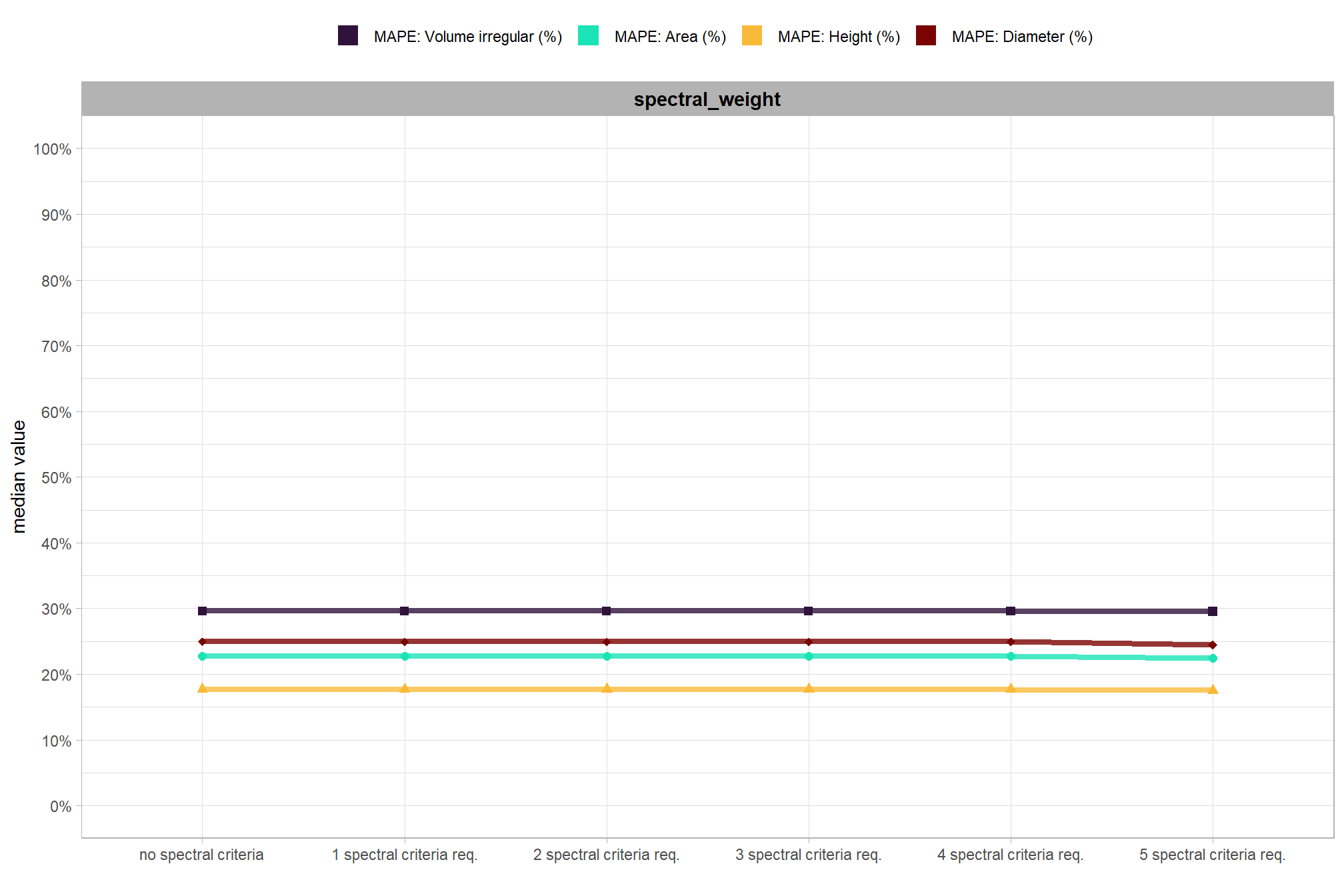
an interesting finding here is that as CHM resolution becomes more coarse, the importance of the spectral data increases (i.e. spectral_weight) for accurately detecting and representing pile form
what is the expected detection accuracy of the top 2.0% (n=141) combinations tested by CHM resolution?
plt_detection_dist2(
  df = param_combos_spectral_ranked %>% dplyr::filter(is_top_chm) %>% dplyr::select(!tidyselect::contains("_pct_rank_"))
  , paste0(
    "Data Fusion"
    , "\ndistribution of pile detection metrics for top "
    , scales::percent(pct_th_top_chm,accuracy=0.1)
    , " (n="
    , scales::comma(n_combos_top_spectral_chm, accuracy=1)
    , ") "
    , "parameter combinations tested by CHM resolution\nbased on both detection and quantification accuracy"
  )
)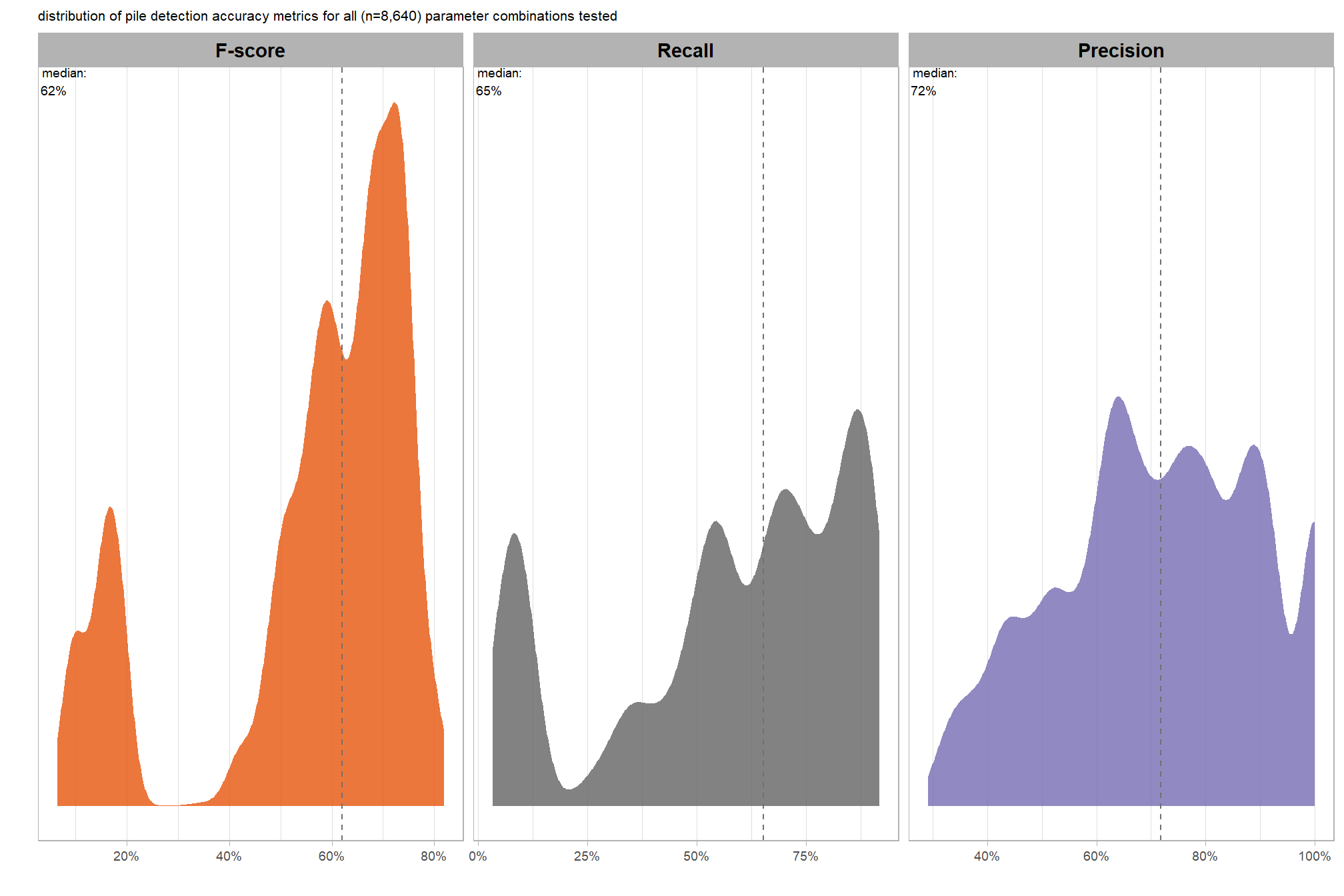
what is the expected MAPE of the top 2.0% (n=141) combinations tested by CHM resolution?
# plot it
plt_form_quantification_dist2(
  df = param_combos_spectral_ranked %>% dplyr::filter(is_top_chm) %>% dplyr::select(!tidyselect::contains("_pct_rank_"))
  , quant_metric = "mape"
  , paste0(
    "Data Fusion"
    , "\ndistribution of pile form quantification metrics for the top "
    , scales::percent(pct_th_top_chm,accuracy=0.1)
    , " (n="
    , scales::comma(n_combos_top_spectral_chm, accuracy=1)
    , ") "
    , "parameter combinations tested by CHM resolution\nbased on both detection and quantification accuracy"
  )
)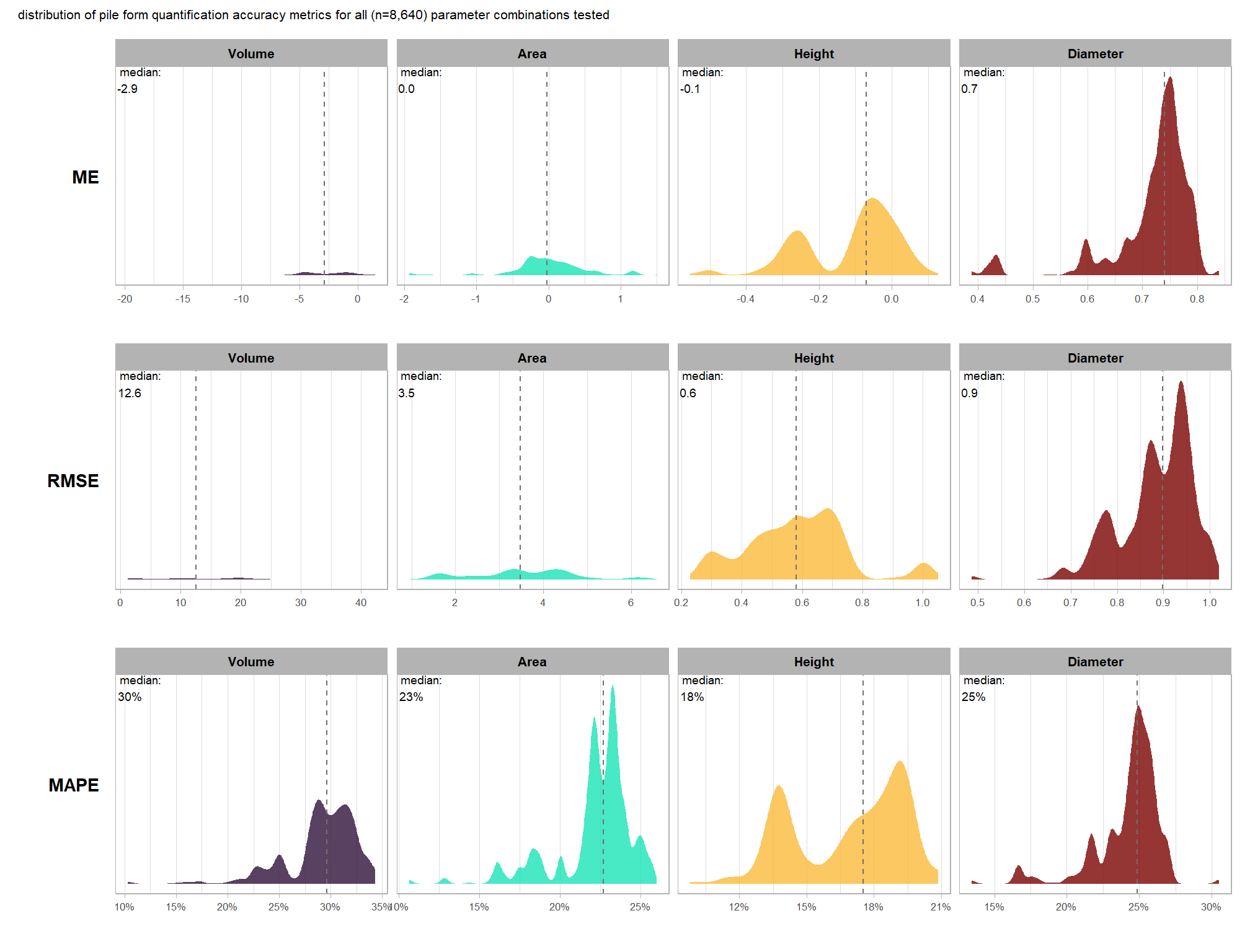
what is the expected Mean Error (ME) of the top 2.0% (n=141) combinations tested by CHM resolution?
# plot it
plt_form_quantification_dist2(
  df = param_combos_spectral_ranked %>% dplyr::filter(is_top_chm) %>% dplyr::select(!tidyselect::contains("_pct_rank_"))
  , quant_metric = "mean"
  , paste0(
    "Data Fusion"
    , "\ndistribution of pile form quantification metrics for the top "
    , scales::percent(pct_th_top_chm,accuracy=0.1)
    , " (n="
    , scales::comma(n_combos_top_spectral_chm, accuracy=1)
    , ") "
    , "parameter combinations tested by CHM resolution\nbased on both detection and quantification accuracy"
  )
)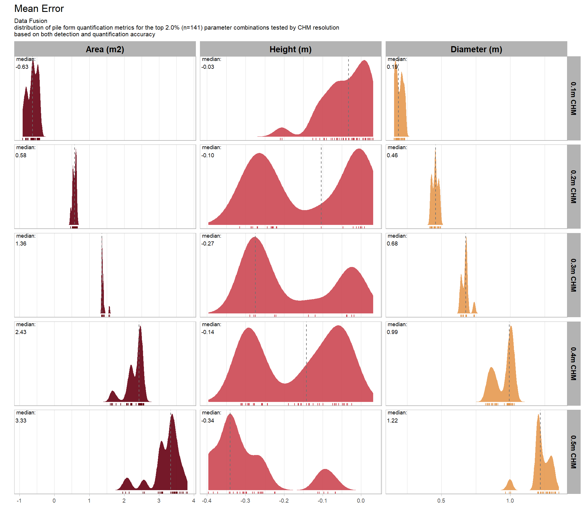
what is the expected RMSE of the top 2.0% (n=141) combinations tested by CHM resolution?
# plot it
plt_form_quantification_dist2(
  df = param_combos_spectral_ranked %>% dplyr::filter(is_top_chm) %>% dplyr::select(!tidyselect::contains("_pct_rank_"))
  , quant_metric = "rmse"
  , paste0(
    "Data Fusion"
    , "\ndistribution of pile form quantification metrics for the top "
    , scales::percent(pct_th_top_chm,accuracy=0.1)
    , " (n="
    , scales::comma(n_combos_top_spectral_chm, accuracy=1)
    , ") "
    , "parameter combinations tested by CHM resolution\nbased on both detection and quantification accuracy"
  )
)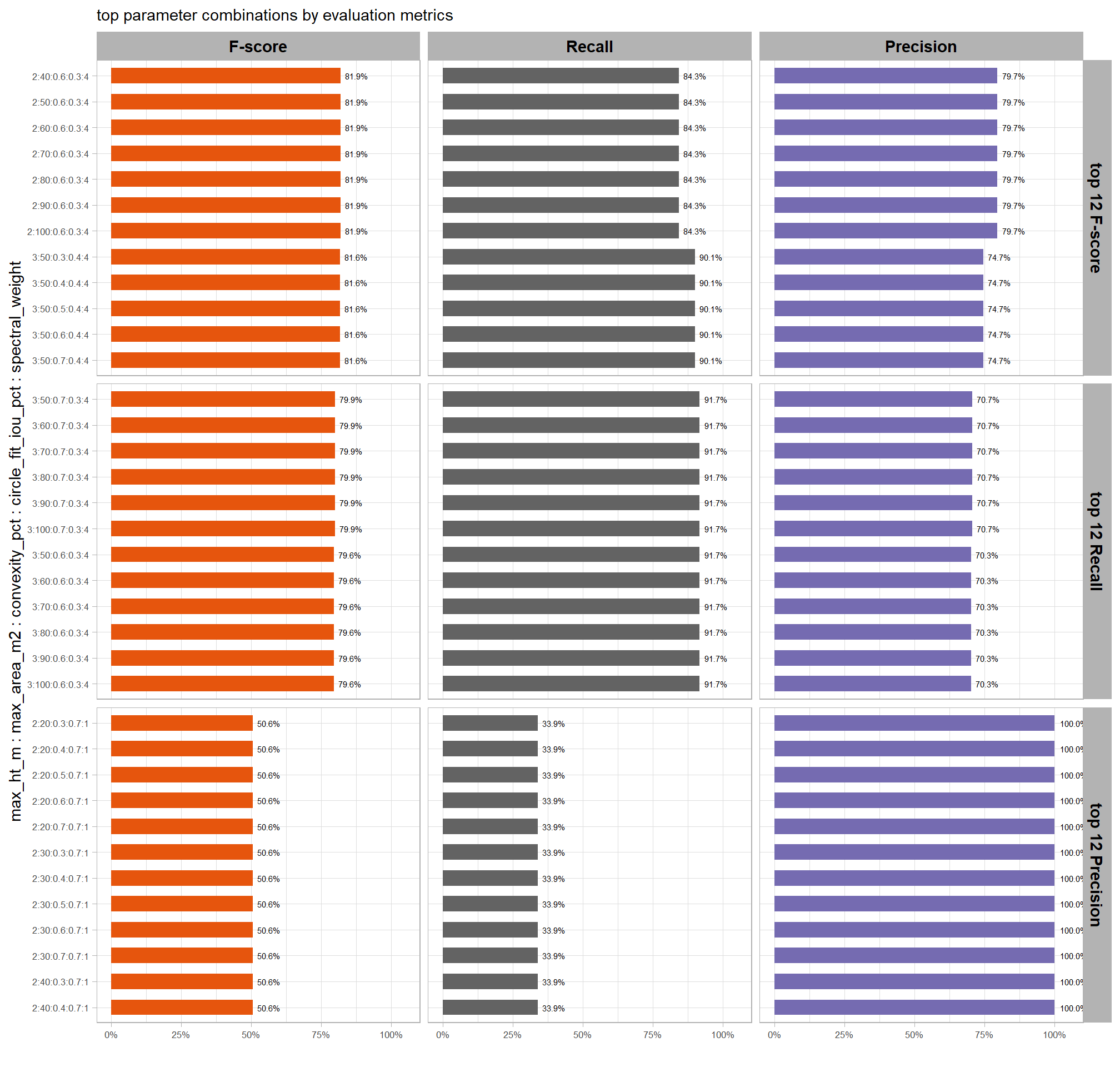
8.6.3.2.2 Final 6 settings
# pal_temp %>% scales::show_col()
# filter and reshape
param_combos_spectral_ranked %>%
  dplyr::filter(is_final_selection_chm) %>%
  dplyr::select(!tidyselect::contains("_pct_rank_")) %>%
  dplyr::select(
    max_ht_m,max_area_m2,convexity_pct,circle_fit_iou_pct,chm_res_m,chm_res_m_desc,spectral_weight
    , chm_lab
    # detection
    , f_score, recall, precision
    # quantification
    , tidyselect::ends_with("_rmse")
    , tidyselect::ends_with("_rrmse")
    , tidyselect::ends_with("_mean")
    , tidyselect::ends_with("_mape")
  ) %>%
  tidyr::pivot_longer(
    cols = c(
      f_score, recall, precision
      , tidyselect::ends_with("_rmse")
      , tidyselect::ends_with("_rrmse")
      , tidyselect::ends_with("_mean")
      , tidyselect::ends_with("_mape")
    )
    , names_to = "metric"
    , values_to = "value"
  ) %>%
  dplyr::mutate(
    eval_metric = stringr::str_extract(metric, "(_rmse|_rrmse|_mean|_mape|f_score|recall|precision)$") %>%
      stringr::str_remove_all("_") %>%
      stringr::str_replace_all("mean","me") %>%
      toupper() %>%
      factor(
        ordered = T
        , levels = c("FSCORE","RECALL","PRECISION", "ME","RMSE","RRMSE","MAPE")
        , labels = c("F-score","Recall","Precision", "ME","RMSE","RRMSE","MAPE")
      )
    , pile_metric = metric %>%
      stringr::str_remove("(_rmse|_rrmse|_mean|_mape)$") %>%
      stringr::str_extract("(paraboloid_volume|volume|area|height|diameter)") %>%
      dplyr::coalesce("detection") %>%
      factor(
        ordered = T
        , levels = c(
          "detection"
          , "volume"
          , "paraboloid_volume"
          , "area"
          , "height"
          , "diameter"
        )
        , labels = c(
          "Detection"
          , "Volume"
          , "Volume paraboloid"
          , "Area (m2)"
          , "Height (m)"
          , "Diameter (m)"
        )
      )
    , value_lab = dplyr::case_when(
        eval_metric %in% c("F-score","Recall","Precision", "RRMSE", "MAPE") ~ scales::percent(value,accuracy=0.1)
        , eval_metric == "ME" ~ scales::comma(value,accuracy=0.01)
        , T ~ scales::comma(value,accuracy=0.1)
      )
  ) %>%
  # make var for color
  dplyr::group_by(chm_res_m,chm_res_m_desc, pile_metric, eval_metric) %>%
  dplyr::mutate(
    # for ME, color by abs...for f-score,recall,precision color by -value so that higher means better...
      # ...since higher means worse for quantification accuracy metrics
    value_dir = dplyr::case_when(
      eval_metric %in% c("ME") ~ abs(value)
      , eval_metric %in% c("F-score","Recall","Precision") ~ -value
      , T ~ value
    )
    , value_z = (value_dir-mean(value_dir,na.rm=T))/sd(value_dir,na.rm=T) # this is the key to the different colors within facets
  ) %>%
  dplyr::ungroup() %>%
  dplyr::filter(!eval_metric %in% c("RRMSE")) %>%
  # View()
  ggplot2::ggplot(mapping = ggplot2::aes(x = eval_metric, y = chm_lab)) +
  ggplot2::geom_tile(
    mapping = ggplot2::aes(fill = pile_metric, alpha = -value_z)
    , color = "gray"
  ) +
  ggplot2::geom_text(
    mapping = ggplot2::aes(label = value_lab, fontface = "bold")
    , color = "white"
    , size = 3
  ) +
  ggplot2::facet_grid(cols = dplyr::vars(pile_metric), rows = dplyr::vars(chm_res_m_desc), scales = "free") +
  ggplot2::scale_x_discrete(position = "top") +
  ggplot2::scale_fill_manual(values = c("gray33", harrypotter::hp(n=3,option = "hermionegranger") )) +
  ggplot2::scale_alpha_binned(range = c(0.55, 1)) + # this is the key to the different colors within facets
  ggplot2::theme_light() +
  ggplot2::labs(
    x = ""
    , y = "max_ht_m : max_area_m2 : convexity_pct : circle_fit_iou_pct : chm_res_m : spectral_weight"
    , subtitle = paste0(
       "Data Fusion"
       , "\npile detection and form quantification accuracy metrics for the top parameter settings tested"
       # , scales::percent(1-pct_rank_th_top,accuracy=1)
       , " (n="
       , scales::comma(n_th_top_chm,accuracy=1)
       , ") by CHM resolution"
       , "\nbased on both detection and quantification accuracy"
      )
    , caption = "*darker colors indicate relatively higher accuracy values"
  ) +
  ggplot2::theme(
    legend.position = "none"
    , panel.grid = ggplot2::element_blank()
    , strip.placement = "outside"
    , strip.text.x = ggplot2::element_text(size = 8, color = "black", face = "bold")
    , strip.text.y = ggplot2::element_text(size = 9, color = "black", face = "bold")
    , axis.text.x = ggplot2::element_text(size = 7, color = "black", face = "bold")
    , axis.text.y = ggplot2::element_text(size = 7)
    , axis.title.x = ggplot2::element_blank()
    , plot.subtitle = ggplot2::element_text(size = 8)
  )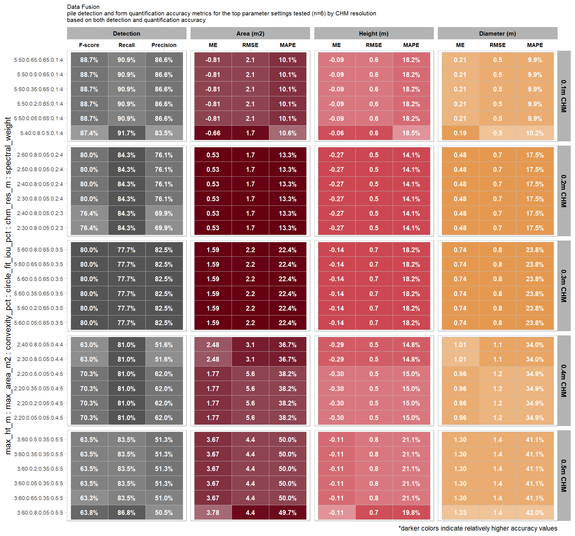
this plot allows for a simultaneous comparison of all metrics for pile detection and pile form quantification. it includes only the parameter combinations that achieved the best balanced accuracy, helping users identify the optimal settings by evaluating the trade-offs between detection and form quantification.
let’s table this
param_combos_spectral_ranked %>%
  dplyr::filter(is_final_selection_chm) %>%
  dplyr::select(!tidyselect::contains("_pct_rank_")) %>%
  # first select to arrange eval_metric
  dplyr::select(
    chm_lab, chm_res_m_desc
    , max_ht_m,max_area_m2,convexity_pct,circle_fit_iou_pct,chm_res_m,spectral_weight
    # detection
    , f_score, recall, precision
    # quantification
    , tidyselect::ends_with("_mean")
    , tidyselect::ends_with("_rmse")
    # , tidyselect::ends_with("_rrmse")
    , tidyselect::ends_with("_mape")
  ) %>%
  # second select to arrange pile_metric
  dplyr::select(
    chm_lab, chm_res_m_desc
    , max_ht_m,max_area_m2,convexity_pct,circle_fit_iou_pct,chm_res_m,spectral_weight
    # detection
    , f_score, recall, precision
    # quantification
    , c(tidyselect::contains("volume") & !tidyselect::contains("paraboloid"))
    , tidyselect::contains("area")
    , tidyselect::contains("height")
    , tidyselect::contains("diameter")
  ) %>%
  # names()
  dplyr::mutate(
    dplyr::across(
      .cols = c(f_score, recall, precision, tidyselect::ends_with("_mape"))
      , .fn = ~ scales::percent(.x, accuracy = 1)
    )
    , dplyr::across(
      .cols = c(tidyselect::ends_with("_mean"))
      , .fn = ~ scales::comma(.x, accuracy = 0.01)
    )
    , dplyr::across(
      .cols = c(tidyselect::ends_with("_rmse"))
      , .fn = ~ scales::comma(.x, accuracy = 0.1)
    )
  ) %>%
  dplyr::mutate(blank= "   " ) %>%
  dplyr::relocate(blank, .before = f_score) %>%
  dplyr::arrange(chm_res_m, desc(chm_lab)) %>%
  dplyr::select(-chm_res_m) %>%
  dplyr::relocate(chm_res_m_desc) %>%
  kableExtra::kbl(
    caption =
      paste0(
       "Data Fusion"
       , "<br>pile detection and form quantification accuracy metrics for the top parameter settings tested"
       # , scales::percent(1-pct_rank_th_top,accuracy=1)
       , " (n="
       , scales::comma(n_th_top_chm,accuracy=1)
       , ") by CHM resolution "
       , "<br>based on both detection and quantification accuracy"
      )
    , col.names = c(
      ".", ""
      ,"max_ht_m","max_area_m2","convexity_pct","circle_fit_iou_pct","spectral_weight"
      , "   "
      , "F-score", "Recall", "Precision"
      , rep(c("ME","RMSE","MAPE"), times = 3)
    )
    , escape = F
  ) %>%
  kableExtra::kable_styling(font_size = 11) %>%
  kableExtra::add_header_above(c(
    " "=8
    , "Detection" = 3
    # , "Volume" = 3
    , "Area" = 3
    , "Height" = 3
    , "Diameter" = 3
  )) %>%
  kableExtra::column_spec(seq(8,20,by=3), border_right = TRUE, include_thead = TRUE) %>%
  kableExtra::column_spec(
    column = 8:20
    , extra_css = "font-size: 10px;"
    , include_thead = T
  ) %>%
  kableExtra::collapse_rows(columns = 1, valign = "top") %>%
kableExtra::scroll_box(width = "740px") | . | max_ht_m | max_area_m2 | convexity_pct | circle_fit_iou_pct | spectral_weight | F-score | Recall | Precision | ME | RMSE | MAPE | ME | RMSE | MAPE | ME | RMSE | MAPE | ||
|---|---|---|---|---|---|---|---|---|---|---|---|---|---|---|---|---|---|---|---|
| 0.1m CHM | 5:50:0.65:0.65:0.1:4 | 5 | 50 | 0.65 | 0.65 | 4 | 89% | 91% | 87% | -0.81 | 2.1 | 10% | -0.09 | 0.6 | 18% | 0.21 | 0.5 | 10% | |
| 5:50:0.5:0.65:0.1:4 | 5 | 50 | 0.50 | 0.65 | 4 | 89% | 91% | 87% | -0.81 | 2.1 | 10% | -0.09 | 0.6 | 18% | 0.21 | 0.5 | 10% | ||
| 5:50:0.35:0.65:0.1:4 | 5 | 50 | 0.35 | 0.65 | 4 | 89% | 91% | 87% | -0.81 | 2.1 | 10% | -0.09 | 0.6 | 18% | 0.21 | 0.5 | 10% | ||
| 5:50:0.2:0.65:0.1:4 | 5 | 50 | 0.20 | 0.65 | 4 | 89% | 91% | 87% | -0.81 | 2.1 | 10% | -0.09 | 0.6 | 18% | 0.21 | 0.5 | 10% | ||
| 5:50:0.05:0.65:0.1:4 | 5 | 50 | 0.05 | 0.65 | 4 | 89% | 91% | 87% | -0.81 | 2.1 | 10% | -0.09 | 0.6 | 18% | 0.21 | 0.5 | 10% | ||
| 5:40:0.8:0.5:0.1:4 | 5 | 40 | 0.80 | 0.50 | 4 | 87% | 92% | 83% | -0.66 | 1.7 | 11% | -0.06 | 0.6 | 19% | 0.19 | 0.5 | 10% | ||
| 0.2m CHM | 2:60:0.8:0.05:0.2:4 | 2 | 60 | 0.80 | 0.05 | 4 | 80% | 84% | 76% | 0.53 | 1.7 | 13% | -0.27 | 0.5 | 14% | 0.48 | 0.7 | 18% | |
| 2:50:0.8:0.05:0.2:4 | 2 | 50 | 0.80 | 0.05 | 4 | 80% | 84% | 76% | 0.53 | 1.7 | 13% | -0.27 | 0.5 | 14% | 0.48 | 0.7 | 18% | ||
| 2:40:0.8:0.05:0.2:4 | 2 | 40 | 0.80 | 0.05 | 4 | 80% | 84% | 76% | 0.53 | 1.7 | 13% | -0.27 | 0.5 | 14% | 0.48 | 0.7 | 18% | ||
| 2:30:0.8:0.05:0.2:4 | 2 | 30 | 0.80 | 0.05 | 4 | 80% | 84% | 76% | 0.53 | 1.7 | 13% | -0.27 | 0.5 | 14% | 0.48 | 0.7 | 18% | ||
| 2:40:0.8:0.05:0.2:3 | 2 | 40 | 0.80 | 0.05 | 3 | 76% | 84% | 70% | 0.53 | 1.7 | 13% | -0.27 | 0.5 | 14% | 0.48 | 0.7 | 18% | ||
| 2:30:0.8:0.05:0.2:3 | 2 | 30 | 0.80 | 0.05 | 3 | 76% | 84% | 70% | 0.53 | 1.7 | 13% | -0.27 | 0.5 | 14% | 0.48 | 0.7 | 18% | ||
| 0.3m CHM | 5:60:0.8:0.65:0.3:5 | 5 | 60 | 0.80 | 0.65 | 5 | 80% | 78% | 82% | 1.59 | 2.2 | 22% | -0.14 | 0.7 | 18% | 0.74 | 0.8 | 24% | |
| 5:60:0.65:0.65:0.3:5 | 5 | 60 | 0.65 | 0.65 | 5 | 80% | 78% | 82% | 1.59 | 2.2 | 22% | -0.14 | 0.7 | 18% | 0.74 | 0.8 | 24% | ||
| 5:60:0.5:0.65:0.3:5 | 5 | 60 | 0.50 | 0.65 | 5 | 80% | 78% | 82% | 1.59 | 2.2 | 22% | -0.14 | 0.7 | 18% | 0.74 | 0.8 | 24% | ||
| 5:60:0.35:0.65:0.3:5 | 5 | 60 | 0.35 | 0.65 | 5 | 80% | 78% | 82% | 1.59 | 2.2 | 22% | -0.14 | 0.7 | 18% | 0.74 | 0.8 | 24% | ||
| 5:60:0.2:0.65:0.3:5 | 5 | 60 | 0.20 | 0.65 | 5 | 80% | 78% | 82% | 1.59 | 2.2 | 22% | -0.14 | 0.7 | 18% | 0.74 | 0.8 | 24% | ||
| 5:60:0.05:0.65:0.3:5 | 5 | 60 | 0.05 | 0.65 | 5 | 80% | 78% | 82% | 1.59 | 2.2 | 22% | -0.14 | 0.7 | 18% | 0.74 | 0.8 | 24% | ||
| 0.4m CHM | 2:40:0.8:0.05:0.4:4 | 2 | 40 | 0.80 | 0.05 | 4 | 63% | 81% | 52% | 2.48 | 3.1 | 37% | -0.29 | 0.5 | 15% | 1.01 | 1.1 | 34% | |
| 2:30:0.8:0.05:0.4:4 | 2 | 30 | 0.80 | 0.05 | 4 | 63% | 81% | 52% | 2.48 | 3.1 | 37% | -0.29 | 0.5 | 15% | 1.01 | 1.1 | 34% | ||
| 2:20:0.5:0.05:0.4:5 | 2 | 20 | 0.50 | 0.05 | 5 | 70% | 81% | 62% | 1.77 | 5.6 | 38% | -0.30 | 0.5 | 15% | 0.96 | 1.2 | 35% | ||
| 2:20:0.35:0.05:0.4:5 | 2 | 20 | 0.35 | 0.05 | 5 | 70% | 81% | 62% | 1.77 | 5.6 | 38% | -0.30 | 0.5 | 15% | 0.96 | 1.2 | 35% | ||
| 2:20:0.2:0.05:0.4:5 | 2 | 20 | 0.20 | 0.05 | 5 | 70% | 81% | 62% | 1.77 | 5.6 | 38% | -0.30 | 0.5 | 15% | 0.96 | 1.2 | 35% | ||
| 2:20:0.05:0.05:0.4:5 | 2 | 20 | 0.05 | 0.05 | 5 | 70% | 81% | 62% | 1.77 | 5.6 | 38% | -0.30 | 0.5 | 15% | 0.96 | 1.2 | 35% | ||
| 0.5m CHM | 3:60:0.5:0.35:0.5:5 | 3 | 60 | 0.50 | 0.35 | 5 | 64% | 83% | 51% | 3.67 | 4.4 | 50% | -0.11 | 0.8 | 21% | 1.30 | 1.4 | 41% | |
| 3:60:0.35:0.35:0.5:5 | 3 | 60 | 0.35 | 0.35 | 5 | 64% | 83% | 51% | 3.67 | 4.4 | 50% | -0.11 | 0.8 | 21% | 1.30 | 1.4 | 41% | ||
| 3:60:0.2:0.35:0.5:5 | 3 | 60 | 0.20 | 0.35 | 5 | 64% | 83% | 51% | 3.67 | 4.4 | 50% | -0.11 | 0.8 | 21% | 1.30 | 1.4 | 41% | ||
| 3:60:0.05:0.35:0.5:5 | 3 | 60 | 0.05 | 0.35 | 5 | 64% | 83% | 51% | 3.67 | 4.4 | 50% | -0.11 | 0.8 | 21% | 1.30 | 1.4 | 41% | ||
| 3:60:0.65:0.35:0.5:5 | 3 | 60 | 0.65 | 0.35 | 5 | 63% | 83% | 51% | 3.67 | 4.4 | 50% | -0.11 | 0.8 | 21% | 1.30 | 1.4 | 41% | ||
| 3:60:0.8:0.05:0.5:5 | 3 | 60 | 0.80 | 0.05 | 5 | 64% | 87% | 50% | 3.78 | 4.4 | 50% | -0.11 | 0.7 | 20% | 1.33 | 1.4 | 42% |
what is the expected detection accuracy of the top 6 settings by CHM resolution?
plt_detection_dist2(
  df = param_combos_spectral_ranked %>% dplyr::filter(is_final_selection_chm) %>% dplyr::select(!tidyselect::contains("_pct_rank_"))
  , paste0(
    "Data Fusion"
    , "\ndistribution of pile detection metrics for the top parameter settings tested"
    , " (n="
    , scales::comma(n_th_top_chm,accuracy=1)
    , ") by CHM resolution"
    , "\nbased on both detection and quantification accuracy"
  )
)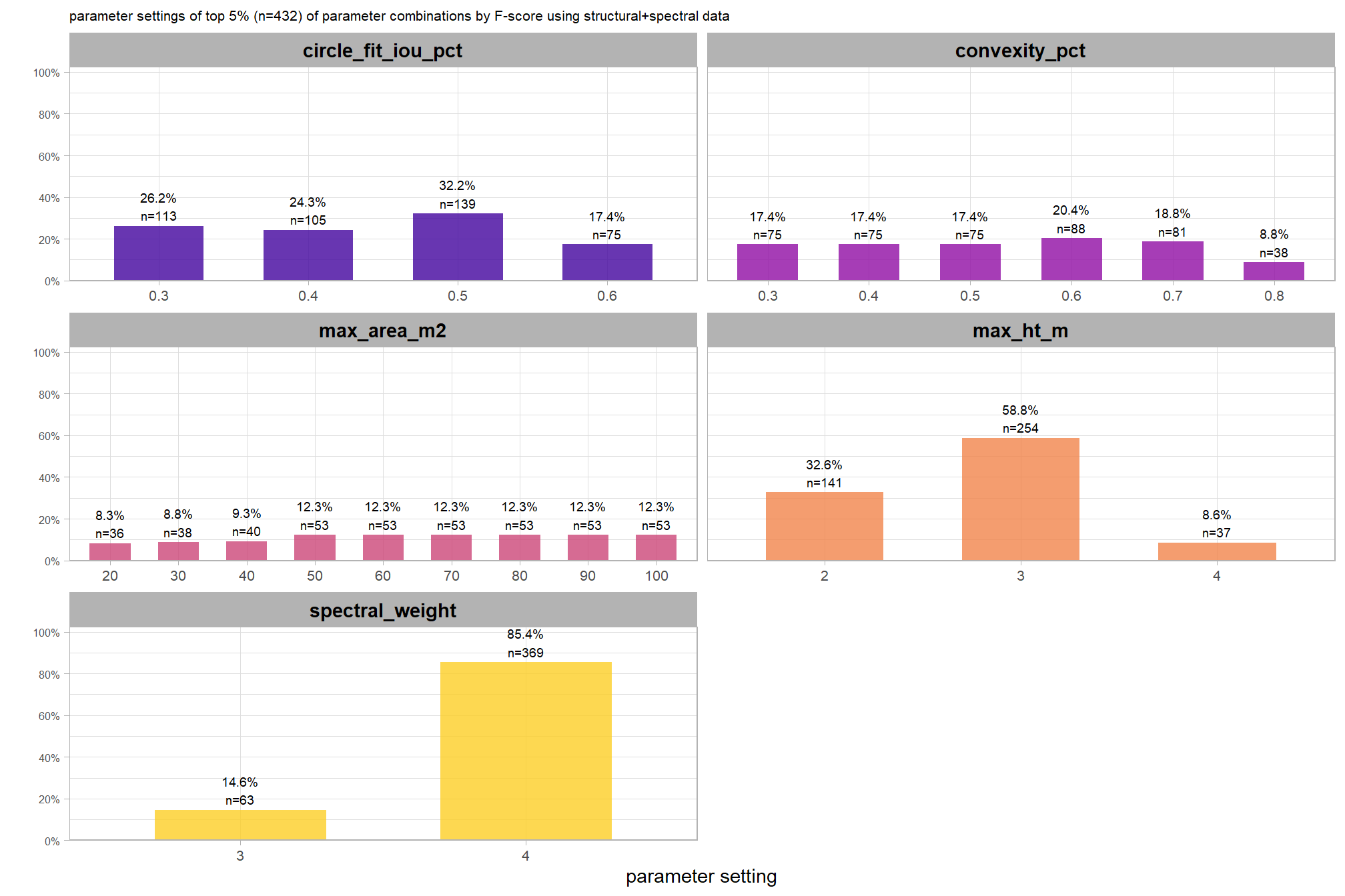
what is the expected MAPE of the top 6 settings by CHM resolution?
# plot it
plt_form_quantification_dist2(
  df = param_combos_spectral_ranked %>% dplyr::filter(is_final_selection_chm) %>% dplyr::select(!tidyselect::contains("_pct_rank_"))
  , quant_metric = "mape"
  , paste0(
    "Data Fusion"
    , "\ndistribution of pile form quantification metrics for the top parameter settings tested"
    , " (n="
    , scales::comma(n_th_top_chm,accuracy=1)
    , ") by CHM resolution"
    , "\nbased on both detection and quantification accuracy"
  )
)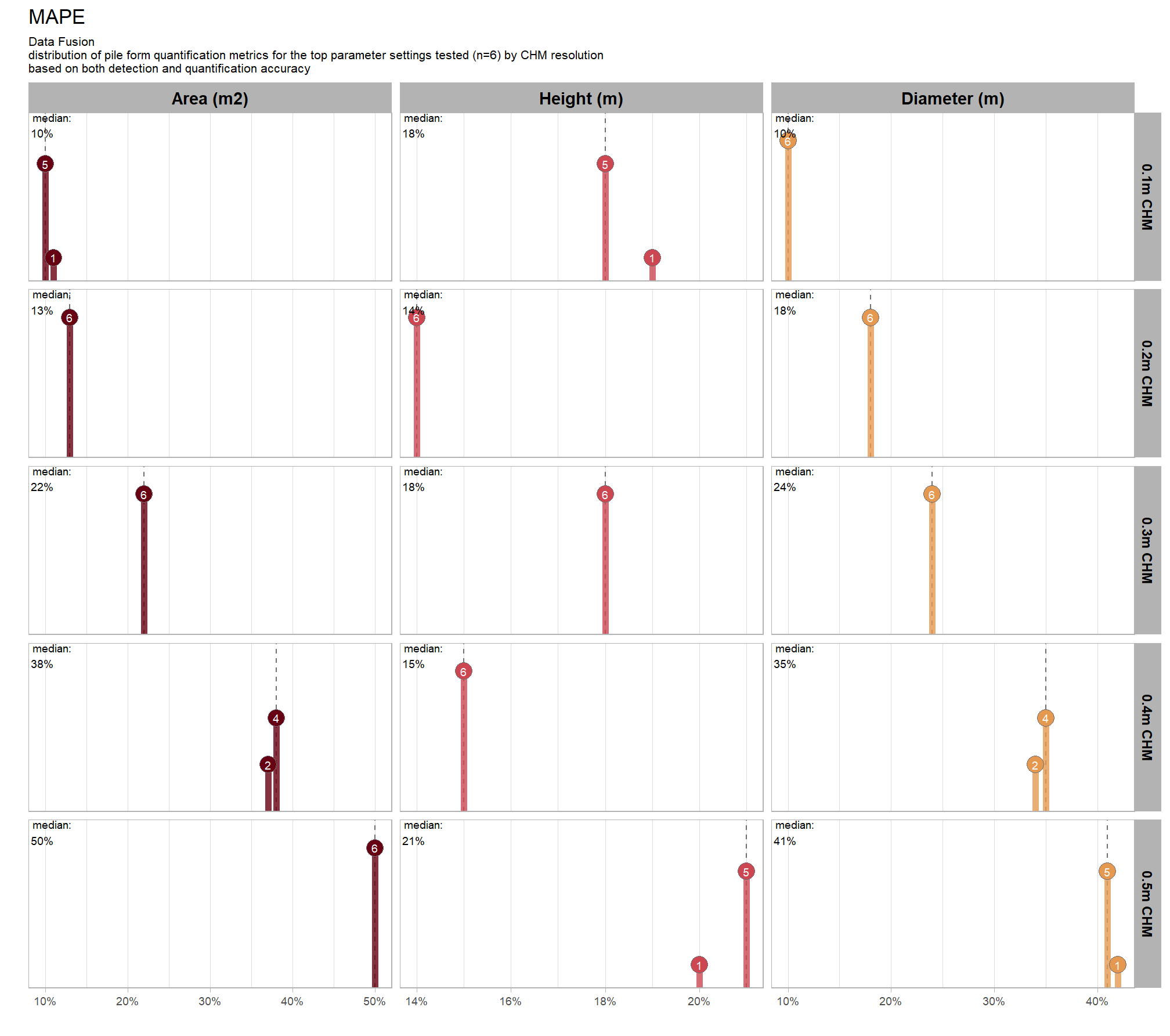
what is the expected Mean Error (ME) of the top 6 settings by CHM resolution?
# plot it
plt_form_quantification_dist2(
  df = param_combos_spectral_ranked %>% dplyr::filter(is_final_selection_chm) %>% dplyr::select(!tidyselect::contains("_pct_rank_"))
  , quant_metric = "mean"
  , paste0(
    "Data Fusion"
    , "\ndistribution of pile form quantification metrics for the top parameter settings tested"
    , " (n="
    , scales::comma(n_th_top_chm,accuracy=1)
    , ") by CHM resolution"
    , "\nbased on both detection and quantification accuracy"
  )
)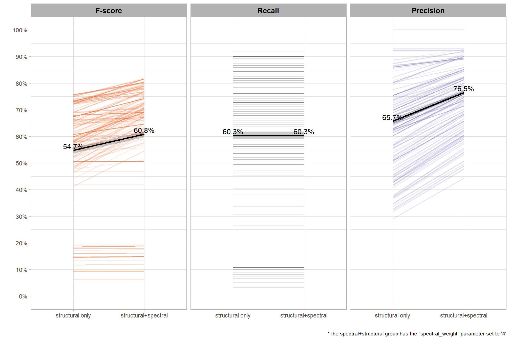
what is the expected RMSE of the top 6 settings by CHM resolution?
# plot it
plt_form_quantification_dist2(
  df = param_combos_spectral_ranked %>% dplyr::filter(is_final_selection_chm) %>% dplyr::select(!tidyselect::contains("_pct_rank_"))
  , quant_metric = "rmse"
  , paste0(
    "Data Fusion"
    , "\ndistribution of pile form quantification metrics for the top parameter settings tested"
    , " (n="
    , scales::comma(n_th_top_chm,accuracy=1)
    , ") by CHM resolution"
    , "\nbased on both detection and quantification accuracy"
  )
)