Section 12 Method Validation: Summary
Lastly, we will examine the aggregated performance achieved by the data fusion approach across all tested study sites. This comparison involves three distinct metric types:
- Detection Accuracy Metrics: These metrics are calculated by aggregating the raw counts of True Positives (TP), False Positives (FP), and False Negatives (FN) from all sites. They quantify the method’s ability to successfully locate and identify the piles.
- Quantification Accuracy Metrics: Calculated for instances classified as TP, these metrics (e.g., RMSE, MAPE, Mean Error) aggregate the differences between the predicted pile attributes (Area, Diameter) and the ground truth values. These metrics assess the method’s ability to accurately quantify the form of the piles it successfully identified.
- Overall Total Quantification Comparison: This involves summarizing the predicted and ground truth pile form measurements (area, diameter) for all instances across the entire study area, regardless of whether individual piles were successfully matched between datasets. This overall comparison provides crucial insight into the method’s aggregated performance in predicting total pile size in an area. Such totals are often required for administrative needs like submitting burn permits which do not typically focus on individual pile quantification differences.
For all form quantification performance assessment, we will rely solely on comparison against image-annotated footprints by comparing predicted diameter and area against the image-annotated values. This consistency is required because image-annotated data is available for all sites, whereas field-measured height and diameter data were only available for the training site.
# read in the file with the aggregated results we wrote in each section
all_agg_ground_truth_match_ans <- readr::read_csv(file = all_agg_ground_truth_match_ans_fp, progress = F, show_col_types = F) %>%
  dplyr::mutate(
    site = ordered(site) %>% forcats::fct_relevel("ponderosa pine training site") %>% forcats::fct_rev()
    , pct_diff_diameter = (pred_diameter_m-image_gt_diameter_m)/image_gt_diameter_m
    , pct_diff_area = (pred_area_m2-gt_area_m2)/gt_area_m2
  )
# huh?
all_agg_ground_truth_match_ans %>% dplyr::glimpse()
## Rows: 3
## Columns: 29
## $ tp_n <dbl> 107, 262, 22
## $ fp_n <dbl> 30, 79, 5
## $ fn_n <dbl> 14, 15, 4
## $ omission_rate <dbl> 0.11570248, 0.05415162, 0.15384615
## $ commission_rate <dbl> 0.2189781, 0.2316716, 0.1851852
## $ precision <dbl> 0.7810219, 0.7683284, 0.8148148
## $ recall <dbl> 0.8842975, 0.9458484, 0.8461538
## $ f_score <dbl> 0.8294574, 0.8478964, 0.8301887
## $ diff_area_m2_rmse <dbl> 2.100498, 1.967614, 49.433509
## $ diff_field_diameter_m_rmse <dbl> 0.5539741, 1.7995497, NA
## $ diff_height_m_rmse <dbl> 0.6546709, 1.2064009, NA
## $ diff_image_diameter_m_rmse <dbl> 0.4440600, 0.4527556, 4.0095773
## $ diff_area_m2_mean <dbl> -0.6315793, -1.1914491, -17.9769566
## $ diff_field_diameter_m_mean <dbl> 0.2124978, -1.7127948, NA
## $ diff_height_m_mean <dbl> -0.2023439, -1.1668889, NA
## $ diff_image_diameter_m_mean <dbl> -0.1723016, -0.2584928, -1.5220128
## $ pct_diff_area_m2_mape <dbl> 0.12012811, 0.14541068, 0.08594908
## $ pct_diff_field_diameter_m_mape <dbl> 0.1121629, 0.3055677, NA
## $ pct_diff_height_m_mape <dbl> 0.1548135, 0.5146757, NA
## $ pct_diff_image_diameter_m_mape <dbl> 0.07706101, 0.08139310, 0.06837243
## $ image_gt_diameter_m <dbl> 463.7905, 1155.4669, 545.7089
## $ pred_diameter_m <dbl> 486.6239, 1274.2344, 539.3018
## $ gt_area_m2 <dbl> 1185.542, 2942.573, 5198.640
## $ pred_area_m2 <dbl> 1121.190, 2846.445, 4808.925
## $ pred_volume_m3 <dbl> 952.529, 1613.947, 5066.225
## $ pred_height_m <dbl> 263.02139, 427.64159, 72.98016
## $ site <ord> ponderosa pine training site, pinyon-ju…
## $ pct_diff_diameter <dbl> 0.04923211, 0.10278747, -0.01174094
## $ pct_diff_area <dbl> -0.05428061, -0.03266808, -0.07496482make a quick plot to look across study sites at the aggregated accuracy metrics
all_agg_ground_truth_match_ans %>%
  dplyr::select(
    site
    ## detection
    ,omission_rate,commission_rate,precision,recall,f_score
    ## quantification
    # ,diff_area_m2_rmse,diff_field_diameter_m_rmse,diff_height_m_rmse,diff_image_diameter_m_rmse
    # ,diff_area_m2_mean,diff_field_diameter_m_mean,diff_height_m_mean,diff_image_diameter_m_mean
    # ,pct_diff_field_diameter_m_mape,pct_diff_height_m_mape
    ,pct_diff_area_m2_mape,pct_diff_image_diameter_m_mape
    ## totals
    # ,image_gt_diameter_m,pred_diameter_m,gt_area_m2,pred_area_m2,site
    ,pct_diff_diameter,pct_diff_area
  ) %>%
  tidyr::pivot_longer(cols = -c(site)) %>%
  dplyr::mutate(
    metric_type = dplyr::case_when(
      name %in% c("omission_rate","commission_rate","precision","recall","f_score") ~ "Detection Accuracy"
      , name %in% c("pct_diff_area_m2_mape","pct_diff_image_diameter_m_mape") ~ "Quantification Accuracy"
      , name %in% c("pct_diff_diameter","pct_diff_area") ~ "Site Aggregate Totals"
      , T ~ "error"
    )
    , label = scales::percent(value, accuracy = 0.1)
    , name = dplyr::case_when(
      name == "f_score" ~ "F-score"
      , stringr::str_starts(name,"pct_diff_") & metric_type == "Site Aggregate Totals" ~ stringr::str_replace_all(name,"pct_diff_","% Diff. ") %>% stringr::str_to_sentence()
      , stringr::str_ends(name,"_mape") ~ stringr::str_extract(name,"(area|diameter)") %>% stringr::str_c(" MAPE")
      , T ~ stringr::str_replace_all(name,"_"," ") %>% stringr::str_to_sentence()
    )
  ) %>%
  dplyr::mutate(
    label = dplyr::case_when(
      metric_type == "Site Aggregate Totals" & value>0 ~ paste0("+", label)
      , T ~ label
    )
    # , label_pos = ifelse(value > 0, 0.005, -0.0073)
    , name2 = forcats::fct_cross(ordered(metric_type),ordered(name), sep = ": ")
  ) %>%
  dplyr::arrange(metric_type, site) %>%
  ggplot2::ggplot(
    mapping = ggplot2::aes(x = value, y = site, color = metric_type, fill = metric_type)
  ) +
  ggplot2::geom_col(
    width = 0.6
    , color = NA
  ) +
  # ggplot2::geom_text(
  #   mapping = ggplot2::aes(label = label, x = label_pos, fontface = "bold")
  #   , vjust = 0
  #   , hjust = 0
  #   , color = "white", size = 3
  # ) +
  ggplot2::geom_text(
    mapping = aes(
      label = ifelse(value<0, label, "")
      , fontface = "bold"
    )
    , color = "black", size = 2
    , hjust = +1
  ) +
  ggplot2::geom_text(
    mapping = aes(
      label = ifelse(value>=0, label, "")
      , fontface = "bold"
    )
    , color = "black", size = 2
    , hjust = 0
  ) +
  ggplot2::facet_wrap(facets = dplyr::vars(name2), ncol = 2, scales = "free") +
  harrypotter::scale_fill_hp_d(option = "ronweasley2", direction = -1) +
  ggplot2::scale_x_continuous(labels = scales::percent, expand = ggplot2::expansion(mult = c(0.1,0.1))) +
  ggplot2::labs(fill = "", x = "", y = "") +
  ggplot2::theme_light() +
  ggplot2::theme(
    legend.position = "top"
    , strip.text = ggplot2::element_text(size = 9, color = "black", face = "bold")
    , axis.text.x = ggplot2::element_text(size = 6)
  )
and a table
all_agg_ground_truth_match_ans %>%
  dplyr::mutate(
    ref_trees = tp_n+fn_n
    , det_trees = tp_n+fp_n
  ) %>%
  dplyr::select(
    site
    , ref_trees
    , det_trees
    , tp_n
    , omission_rate,commission_rate,recall,precision,f_score
    , pct_diff_area_m2_mape
    , pct_diff_area
  ) %>%
  dplyr::mutate(
    dplyr::across(
      .cols = c(omission_rate,commission_rate,recall,precision,f_score)
      , .fns = ~scales::percent(.x,accuracy=0.1)
    )
    , pct_diff_area_m2_mape = scales::percent(pct_diff_area_m2_mape,accuracy=0.1)
    , pct_diff_area = scales::percent(pct_diff_area,accuracy=0.1)
  ) %>%
  dplyr::arrange(desc(site)) %>%
  kableExtra::kbl(
    caption = "Data fusion method slash pile segmentation results for each study site"
    , col.names = c(
      "site"
      , "reference<br>piles", "detected<br>piles", "correct<br>piles"
      , "omission<br>rate"
      , "commission<br>rate"
      ,"recall","precision","F-score"
      , "MAPE<br>area m<sup>2</sup>"
      , "% aggregated<br>area difference"
    )
    , escape = F
  ) %>%
  kableExtra::kable_styling(font_size = 10) %>%
kableExtra::collapse_rows(columns = 1, valign = "top")| site |
reference piles |
detected piles |
correct piles |
omission rate |
commission rate |
recall | precision | F-score |
MAPE area m2 |
% aggregated area difference |
|---|---|---|---|---|---|---|---|---|---|---|
| ponderosa pine training site | 121 | 137 | 107 | 11.6% | 21.9% | 88.4% | 78.1% | 82.9% | 12.0% | -5.4% |
| BHEF ponderosa pine validation site | 26 | 27 | 22 | 15.4% | 18.5% | 84.6% | 81.5% | 83.0% | 8.6% | -7.5% |
| pinyon-juniper validation site | 277 | 341 | 262 | 5.4% | 23.2% | 94.6% | 76.8% | 84.8% | 14.5% | -3.3% |
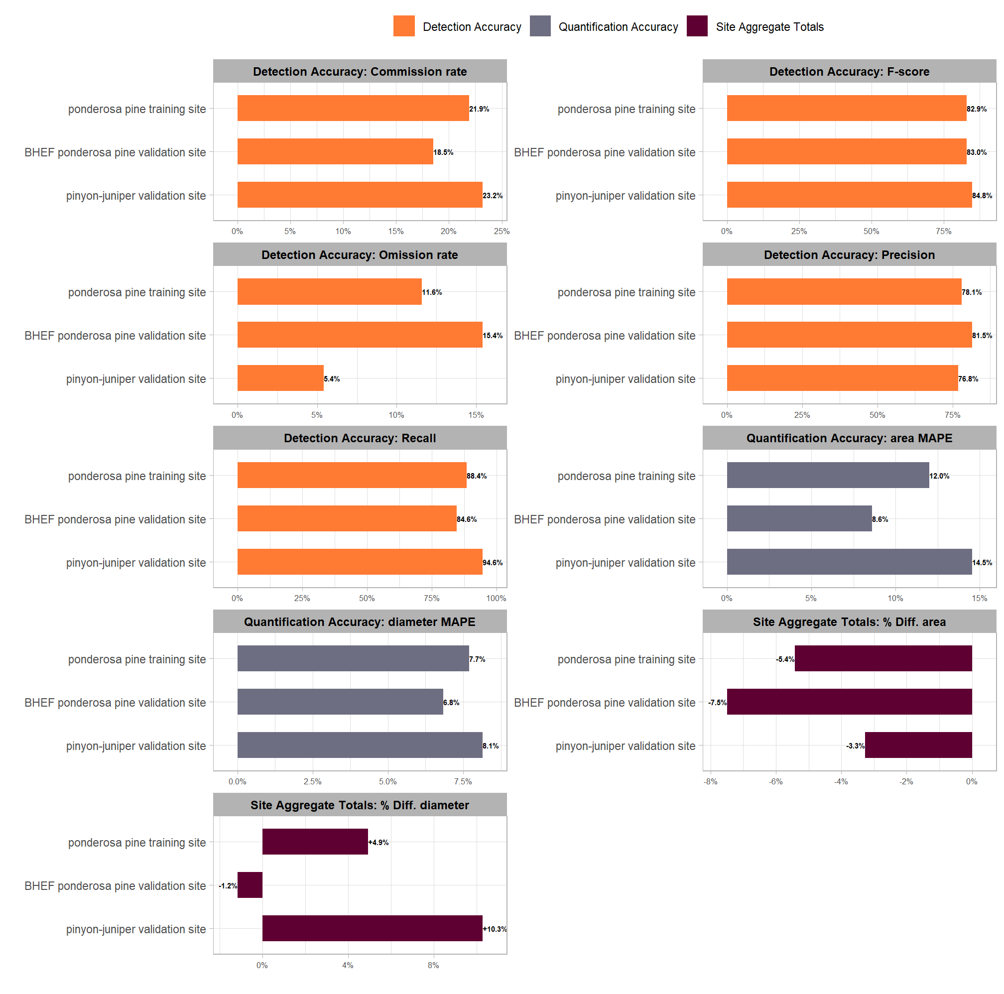
The aggregated results across all three study sites, including the complex, out-of-sample validation sites, demonstrate the consistent transferability and dependability of our data fusion slash pile methodology. All sites achieved consistently high detection performance, with F-scores ranging narrowly from 83% to 85%, confirming the method’s overall effectiveness despite vast differences in pile sizes, vegetation, terrain, and construction techniques.
The specific composition of errors (false positives and false negatives) highlights the success of the site-specific parameter adjustments. The pinyon-juniper validation site (277 piles) recorded the highest F-score (85%), driven by a very high recall rate (95%) which suggests the structural parameters effectively located the many smaller, hand-piled objects, even with less restrictive structural filters. However, this high recall came at the expense of the lowest precision (77%), confirming our observation that the spectral filter failed to exclude numerous false positives (FPs) because the site’s senescent, arid vegetation mimicked the spectral signature of dead wood in piles. In contrast, the BHEF ponderosa pine evaluation site (26 piles) achieved a strong F-score (83%) which is notable given the low pile count amplifies the influence of each error. This site had the lowest recall (85%) due to the complexities of segmenting the massive, irregular pile shapes, but it maintained the highest precision (81%), demonstrating that the strict spectral filtering (spectral_weight set to its maximum value of ‘5’) successfully minimized FPs from the dense ponderosa pine regeneration groups, validating that parameter choice for environments with dense regeneration or shrub cover.
Consistent pile form quantification accuracy indicates the method reliably extracts of pile form measurements (e.g., area, height) for use in planning the management of the piles. The MAPE on pile area, which measures the average error in sizing individual, successfully matched piles, was below 15% across all sites, ranging from 9% to 15%. This result suggests that the methodology can consistently quantify the form of individual piles with high accuracy regardless of the extensive differences in pile sizes, terrain, and construction forms. The BHEF ponderosa pine evaluation site recorded the lowest MAPE on pile area (9%), meaning the piles it did find were sized most accurately of the sites measured.
Analysis of the site aggregate totals revealed a systematic underprediction of the total area across all sites. This systematic underestimation, with errors ranging only from -7.5% to -3.3%, is an important result for administrative needs (such as burn permits), as it avoids overstating the total quantity of fuel (area or volume) on a site. The BHEF ponderosa pine evaluation site had the largest aggregate pile area underestimation (-7.5%). This was likely caused by lower recall rates resulting from the watershed algorithm splitting single massive piles due to their irregular elevation profile or from CHM artifacts produced by cloud cover and SfM flight stitching. The pinyon-juniper site had the highest individual pile area MAPE (14.5%), indicating the worst individual sizing accuracy, but it achieved the closest match to the true total pile area over the entire site (-3.3%), implying that the individual sizing errors of the retained piles compensated for each other across the entire site extent.