Section 10 Method Validation: Pinyon-Juniper
This project has progressed through several phases to develop and validate a rigorous rules-based methodology for slash pile detection.
Phase 1: Methodology Development and Sensitivity Testing This phase involved using ground truth data to perform sensitivity testing on the rules-based detection methodology. We first demonstrated a structural-only method, which uses a CHM raster generated from aerial point cloud data to identify candidate piles based on structural metrics like height, area, and shape. This method can be used when spectral data is unavailable. We then demonstrated a data fusion approach, which builds on the structural method by integrating spectral data as an additional filtering step. This approach takes the structurally-detected candidates and filters out potential false positive predictions by applying a set of spectral index thresholds. We then performed parameter sensitivity testing to systematically vary parameterizations on both approaches and quantify the resulting changes in detection and form quantification accuracy. This sensitivity testing provided a set of individual point estimates of detection accuracy (F-score) and quantification accuracy (e.g. RMSE and MAPE) for each parameter combination tested. These point estimates then served as the input dataset for subsequent statistical modeling to quantify the influence of parameters and input data on accuracy.
Phase 2: Statistical Modeling Following sensitivity testing, a Bayesian Generalized Linear Model (GLM) was used to build a statistical framework for understanding the methodology’s performance. Unlike the sensitivity testing, which generate a range of detection and quantification accuracies based on parameter combinations tested, the statistical modeling does not calculate accuracy itself but instead uses these point estimates as dependent variables to statistically model the functional relationship between the tested detection parameters and the resulting accuracy. This provided a principled way to understand uncertainty and the complex interactions between parameters by providing posterior distributions for each parameter estimate rather than simple point estimates as obtained via sensitivity testing. This statistical modeling enabled the quantification of Bayesian credible intervals, which provide a direct measure of the uncertainty in each relationship, and allowed us to explicitly model interactions between parameters (e.g., the combined effect of CHM resolution and spectral data). Understanding these relationships and their associated uncertainty is critical for making more informed and confident decisions about the method’s optimal settings.
Phase 3: Method Validation
The final phase of this study involves two distinct validation sites to assess the methodology’s real-world generalizability and transferability. Crucially, our detection methodology’s parameter setup (e.g., initial size and shape filters) will be adjusted for each validation site based on its unique treatment and pile construction prescription, mimicking real-life application where optimal settings vary by implementation and forest type.
The validation will use two sites with fundamentally different pile structures:
- Pinyon-Juniper Site: Features smaller, hand-piles only.
- Massive Machine Pile Site (Validation Ponderosa Pine): Features massive machine piles that exhibit high geometric irregularity, with perimeters ranging from circular to rectangular, representing structures significantly larger and more geometrically distinct than those in the training data.
The unreliability of the field-measured height and diameter data was only discovered when initial prediction comparisons failed to meet expectations set by the training data. Consequently, all quantification performance assessment will now be based solely on comparison against image-annotated footprints. This includes:
- Detection Accuracy: Comparing predicted pile locations against image-annotation locations (using metrics like F-score).
- Form Quantification Accuracy: Comparing predicted diameter and area against the image-annotated values (using metrics like MAPE).
The application of the methodology to these structurally distinct, unseen sites—ranging from hand piles to massive machine piles with complex geometries—will provide compelling evidence of its transferability. Acceptable performance despite the challenges posed by differing forest types, terrain, and construction prescriptions will confirm the method’s viability across diverse forest management environments.
10.1 Site Introduction
The present section will validate the detection methodology against a Pinyon-Juniper validation site, employing the detection methodology as informed by the best-performing parameterization using the training data. This validation site is ecologically distinct from the Ponderosa Pine training area, featuring typically denser stands composed of smaller trees and an increased shrub presence, creating a more complex background canopy structure. Furthermore, this site exclusively utilized hand-piling for slash treatment, producing smaller piles than the few machine piles in the training data. To effectively assess the method’s transferability, the detection methodology’s parameters will be adjusted from the training site’s optimal settings based on the specific treatment prescription and onsite implementation feedback, mimicking real-world application where site conditions and methods directly influence pile characteristics. Ground truth validation data from the Pinyon-Juniper site will be used to calculate performance metrics (e.g., F-score and MAPE) to determine how well the method generalizes; if the resulting accuracy is acceptable despite these ecological and structural challenges, it would provide compelling evidence that the methodology is transferable across different forest types.
from field crew leader (G.O.):
Height and width were measured with a retractable height pole from the north side of each pile. We completed all piles (to the best of our knowledge) in the uniform high portion of unit 10. The prescription called for 30 ft spacing between trees and minimum 5x5x5 ft piles. As you can see from the photos and pile dimensions, there are no piles even remotely close to being that small. Others on the project expressed that they were too big. Lastly, no piles had been burned in the unit. The CRS is NAD83(2011) / UTM zone 13N (EPSG:6342). U10 is the highlighted one in the screenshot, but the unit shape file is attached as well.
10.2 Data Processing
10.2.1 Vector Data
load vector data
pile point locations were collected on the ground using highly accurate Emlid Reach RTK-GPS units. The perimeter of each pile was then digitized in a Geographic Information System (GIS) using these point locations overlaid on a 0.026 m RGB orthomosaic. In this digitization process, the perimeter was based on the main footprint of the pile at ground level, excluding isolated logs or debris extending beyond the primary boundary. These ground truth polygons will be compared to the predicted pile boundaries using the intersection over union (IoU) metric, with a minimum threshold required for a true positive match.
# these piles were collected twice in the same location and have different measurements :\
bad_pile_ids <- c(
  142
  , 146
  , 99
  , 96
  , 50
)
###############################################################
# read pile points collected in field
###############################################################
pj_slash_piles_points <- readr::read_csv("../data/Dawson_data/PJ_Piles_Unit_10.csv") %>%
  dplyr::rename_with(tolower) %>%
  dplyr::rename_with(stringr::str_squish) %>%
  dplyr::rename_with(make.names) %>%
  dplyr::rename_with(~stringr::str_replace_all(.x, "\\.{2,}", ".")) %>%
  dplyr::rename_with(~stringr::str_remove(.x, "\\.$")) %>%
  dplyr::rename_with(~stringr::str_replace_all(.x, "\\.", "_")) %>%
  dplyr::mutate(
    pile_id = tidyr::extract_numeric(name)
  ) %>%
  dplyr::filter(
    !(pile_id %in% bad_pile_ids)
  )
pj_slash_piles_points %>% dplyr::glimpse()
## Rows: 274
## Columns: 40
## $ name <chr> "Pile 1", "Pile 2", "Pile 3", "Pile 4", "Pile …
## $ height_m <dbl> 2.12, 1.90, 1.80, 1.90, 2.10, 2.30, 2.00, 2.50…
## $ width_m <dbl> 6.20, 5.70, 4.50, 4.60, 5.60, 6.20, 5.30, 5.40…
## $ code <lgl> NA, NA, NA, NA, NA, NA, NA, NA, NA, NA, NA, NA…
## $ easting <dbl> 180356.3, 180371.2, 180374.8, 180382.1, 180391…
## $ northing <dbl> 4197064, 4197059, 4197050, 4197054, 4197043, 4…
## $ elevation <dbl> 2166.320, 2165.338, 2165.820, 2165.022, 2165.5…
## $ description <lgl> NA, NA, NA, NA, NA, NA, NA, NA, NA, NA, NA, NA…
## $ longitude <dbl> -108.6334, -108.6333, -108.6332, -108.6331, -1…
## $ latitude <dbl> 37.86502, 37.86497, 37.86490, 37.86493, 37.864…
## $ ellipsoidal_height <dbl> 2166.320, 2165.338, 2165.820, 2165.022, 2165.5…
## $ origin <chr> "Global", "Global", "Global", "Global", "Globa…
## $ easting_rms <dbl> 0.087, 0.038, 0.066, 0.073, 0.014, 0.016, 0.03…
## $ northing_rms <dbl> 0.058, 0.082, 0.116, 0.023, 0.022, 0.016, 0.02…
## $ elevation_rms <dbl> 0.011, 0.010, 0.012, 0.011, 0.010, 0.010, 0.01…
## $ lateral_rms <dbl> 0.105, 0.091, 0.134, 0.077, 0.026, 0.023, 0.04…
## $ antenna_height <dbl> 2.134, 2.134, 2.134, 2.134, 2.134, 2.134, 2.13…
## $ antenna_height_units <chr> "m", "m", "m", "m", "m", "m", "m", "m", "m", "…
## $ solution_status <chr> "FIX", "FIX", "FIX", "FIX", "FIX", "FIX", "FIX…
## $ correction_type <chr> "RTK", "RTK", "RTK", "RTK", "RTK", "RTK", "RTK…
## $ averaging_start <chr> "2025-05-30 13:18:45.8 UTC-06:00", "2025-05-30…
## $ averaging_end <chr> "2025-05-30 13:18:55.8 UTC-06:00", "2025-05-30…
## $ samples <dbl> 51, 51, 51, 51, 51, 51, 51, 51, 51, 51, 51, 51…
## $ pdop <dbl> 1.1, 1.1, 1.1, 1.1, 1.1, 1.1, 1.1, 1.1, 1.3, 1…
## $ gdop <dbl> 1.2, 1.3, 1.2, 1.3, 1.2, 1.2, 1.2, 1.2, 1.5, 1…
## $ base_easting <dbl> 180353.5, 180353.5, 180353.5, 180353.5, 180353…
## $ base_northing <dbl> 4197071, 4197071, 4197071, 4197071, 4197071, 4…
## $ base_elevation <dbl> 2168.024, 2168.024, 2168.024, 2168.024, 2168.0…
## $ base_longitude <dbl> -108.6335, -108.6335, -108.6335, -108.6335, -1…
## $ base_latitude <dbl> 37.86507, 37.86507, 37.86507, 37.86507, 37.865…
## $ base_ellipsoidal_height <dbl> 2168.024, 2168.024, 2168.024, 2168.024, 2168.0…
## $ baseline <dbl> 6.968, 21.397, 29.772, 33.082, 46.927, 61.878,…
## $ mount_point <lgl> NA, NA, NA, NA, NA, NA, NA, NA, NA, NA, NA, NA…
## $ cs_name <chr> "NAD83(2011) / UTM zone 13N", "NAD83(2011) / U…
## $ gps_satellites <dbl> 9, 9, 9, 9, 9, 9, 9, 9, 8, 8, 8, 8, 8, 8, 8, 9…
## $ glonass_satellites <dbl> 7, 7, 7, 7, 7, 7, 7, 7, 8, 8, 8, 8, 8, 8, 8, 7…
## $ galileo_satellites <dbl> 8, 8, 8, 8, 8, 8, 8, 8, 9, 8, 9, 9, 8, 8, 7, 8…
## $ beidou_satellites <dbl> 6, 6, 6, 6, 6, 6, 6, 6, 5, 5, 5, 5, 6, 6, 5, 6…
## $ qzss_satellites <dbl> 0, 0, 0, 0, 0, 0, 0, 0, 0, 0, 0, 0, 0, 0, 0, 0…
## $ pile_id <dbl> 1, 2, 3, 4, 5, 6, 7, 8, 9, 10, 11, 12, 13, 14,…pj_slash_piles_points <- pj_slash_piles_points %>%
sf::st_as_sf(coords = c("easting","northing"), crs = 6342, remove = F) %>%
# sf::st_as_sf(coords = c("longitude","latitude"), crs = 4326) %>%
# mapview::mapview(zcol = "height..m.")
dplyr::select(pile_id,name,height_m,width_m,easting,northing,latitude,longitude,code,description,elevation) %>%
sf::st_make_valid()
# sf::st_write("N:/MyFiles/Dawson_data/pj_piles_unit_10.gpkg", append = F)
# mapview::mapview(pj_slash_piles_points, zcol = "height_m")
###############################################################
# read unit boundary
###############################################################
pj_stand_boundary <- sf::st_read("../data/Dawson_data/units/units.shp", quiet=T) %>%
dplyr::rename_with(tolower) %>%
dplyr::rename_with(stringr::str_squish) %>%
dplyr::rename_with(make.names) %>%
dplyr::rename_with(~stringr::str_replace_all(.x, "\\.{2,}", ".")) %>%
dplyr::rename_with(~stringr::str_remove(.x, "\\.$")) %>%
dplyr::rename_with(~stringr::str_replace_all(.x, "\\.", "_")) %>%
sf::st_transform(sf::st_crs(pj_slash_piles_points)) %>%
dplyr::filter(tolower(unit)=="u10") %>%
dplyr::slice(1)what is the area of the treatment unit boundaries we are looking over?
pj_stand_boundary %>%
  sf::st_area() %>%
  as.numeric() %>%
  `/`(10000) %>%
  scales::comma(suffix = " ha", accuracy = 0.01)
## [1] "5.18 ha"that’s great
now load in the pile boundary polygons. because each point does not necessarily fall within the polygon boundary (e.g. due to misalignment between the imagery and point locations or slight inaccuracies in either the point or pile boundaries) we need to perform a matching process to tie the points to the polygons so that we get the height and diameter measured during the point collection attached to the polygons. to do this, we’ll use a two-stage process that first attaches the points data frame to polygons where points fall within, using a spatial intersection. It then finds and assigns the remaining, unjoined points to their nearest polygon. The final output includes all polygons from the original data, ensuring that every polygon is represented even if no points were matched.
# read in polys
pj_slash_piles_polys <- sf::st_read("../data/Dawson_Data/piles/pj_pile_polys.shp", quiet=T) %>%
  # sf::st_as_sf() %>%
  dplyr::rename_with(tolower) %>%
  dplyr::mutate(
    row_number = dplyr::row_number()
    , treeID = dplyr::row_number()
  ) %>%
  cloud2trees::simplify_multipolygon_crowns() %>%
  dplyr::select(-c(treeID,id)) %>%
  dplyr::filter(row_number!=62)

# pj_slash_piles_polys %>% dplyr::glimpse()
# pj_slash_piles_polys %>% ggplot()+geom_sf()+geom_sf(data=pj_slash_piles_points)

# function to perform a two-step spatial join
  # first matching points that fall inside polygons and
  # then assigning the remaining points to the nearest polygon
  # all original polygons are returned in the final output
# let's do it
pj_slash_piles_polys <- match_points_to_polygons(
    points_sf = pj_slash_piles_points
    , polygons_sf = pj_slash_piles_polys
    , point_id = "pile_id"
    , polygon_id = "row_number"
  ) %>%
  dplyr::ungroup() %>%
  sf::st_make_valid() %>%
  dplyr::filter(sf::st_is_valid(.)) %>%
  # calculate area and volume
  dplyr::mutate(
    field_diameter_m = width_m
    , field_radius_m = (field_diameter_m/2)
    , image_gt_area_m2 = sf::st_area(.) %>% as.numeric()
    # , field_gt_area_m2 = pi*field_radius_m^2
    # volume
    , image_gt_volume_m3 = (1/8) * pi * ( (sqrt(image_gt_area_m2/pi)*2)^2 ) * height_m # (1/8) * pi * (shape_length^2) * max_height_m
      # (sqrt(image_gt_area_m2/pi)*2) = diameter assuming of circle covering same area
    , field_gt_volume_m3 = (1/8) * pi * (field_diameter_m^2) * height_m # (1/8) * pi * (shape_length^2) * max_height_m
  ) %>%
  # area
  st_calculate_diameter() %>%
  dplyr::rename(
    image_gt_diameter_m = diameter_m
  ) %>%
  # fix blank pile_id
  dplyr::mutate(
    pile_id = dplyr::case_when(
      is.na(pile_id) ~ max(pile_id,na.rm = T)+1000+row_number
      , T ~ pile_id
    )
  )

# add a flag for if a pile is in the stand or not based on a spatial intersection
pj_slash_piles_polys <- pj_slash_piles_polys %>%
  dplyr::left_join(
    pj_slash_piles_polys %>%
      sf::st_intersection(
        pj_stand_boundary %>%
          sf::st_transform(sf::st_crs(pj_slash_piles_polys))
      ) %>%
      sf::st_drop_geometry() %>%
      dplyr::distinct(pile_id) %>%
      dplyr::mutate(is_in_stand=T)
    , by = "pile_id"
  ) %>%
  dplyr::mutate(is_in_stand=dplyr::coalesce(is_in_stand, F))
huh?
## Rows: 277
## Columns: 20
## $ row_number          <int> 1, 2, 3, 4, 5, 6, 7, 8, 9, 10, 11, 12, 13, 14, 15,…
## $ pile_id             <dbl> 150, 149, 151, 152, 145, 144, 178, 143, 147, 141, …
## $ name                <chr> "Pile 150", "Pile 149", "Pile 151", "Pile 152", "P…
## $ height_m            <dbl> 2.38, 2.55, 2.50, 2.11, 2.51, 2.31, 3.00, 2.39, 2.…
## $ width_m             <dbl> 6.24, 6.72, 6.38, 5.75, 5.13, 5.53, 6.55, 5.46, 6.…
## $ easting             <dbl> 180146.7, 180151.7, 180139.5, 180145.2, 180155.8, …
## $ northing            <dbl> 4197109, 4197101, 4197095, 4197089, 4197087, 41970…
## $ latitude            <dbl> 37.86535, 37.86528, 37.86521, 37.86517, 37.86515, …
## $ longitude           <dbl> -108.6358, -108.6358, -108.6359, -108.6358, -108.6…
## $ code                <lgl> NA, NA, NA, NA, NA, NA, NA, NA, NA, NA, NA, NA, NA…
## $ description         <lgl> NA, NA, NA, NA, NA, NA, NA, NA, NA, NA, NA, NA, NA…
## $ elevation           <dbl> 2171.823, 2172.045, 2172.957, 2173.210, 2172.660, …
## $ field_diameter_m    <dbl> 6.24, 6.72, 6.38, 5.75, 5.13, 5.53, 6.55, 5.46, 6.…
## $ field_radius_m      <dbl> 3.120, 3.360, 3.190, 2.875, 2.565, 2.765, 3.275, 2…
## $ image_gt_area_m2    <dbl> 13.595434, 15.383318, 10.232298, 13.364827, 12.325…
## $ image_gt_volume_m3  <dbl> 16.178567, 19.613730, 12.790373, 14.099893, 15.468…
## $ field_gt_volume_m3  <dbl> 36.39201, 45.22084, 39.96145, 27.39542, 25.93990, …
## $ geometry            <POLYGON [m]> POLYGON ((707958.5 4193509,..., POLYGON ((…
## $ image_gt_diameter_m <dbl> 4.728407, 5.192360, 4.276639, 4.549041, 4.469193, …
## $ is_in_stand         <lgl> TRUE, TRUE, TRUE, TRUE, TRUE, TRUE, TRUE, TRUE, TR…
map
10.2.2 RGB Data
RGB
###############################################################
# read/crop RGB raster
###############################################################
rgb_fnm_temp <- "../data/dawson_data/dawson_rgb.tif"
if(!file.exists(rgb_fnm_temp)){
  # terra handles large files on disk automatically
  rgb_rast_temp <- terra::rast("d:/BLM_CO_SWDF_DawsonFuelsTreatment/Final/Ortho/BLM_CO_SWDF_DawsonFuelsTreatment_Ortho_202504.tif")
  # Read the polygon file (e.g., a shapefile)
  polygon_border_temp <- pj_stand_boundary %>%
    sf::st_buffer(50) %>%
    sf::st_bbox() %>%
    sf::st_as_sfc() %>%
    sf::st_as_sf() %>%
    terra::vect() %>%
    terra::project(terra::crs(rgb_rast_temp))
  # Crop the raster to the rectangular extent of the polygon
  # Specify a filename to ensure the result is written to disk
  crop_rgb_rast_temp <- terra::crop(rgb_rast_temp, polygon_border_temp, filename =  tempfile(fileext = ".tif"), overwrite = TRUE)
  # Mask the cropped raster to the precise shape of the polygon
  # This function will also be processed on disk due to the file size
  pj_rgb_rast <- terra::mask(crop_rgb_rast_temp, polygon_border_temp, filename = rgb_fnm_temp, overwrite = TRUE)
}else{
  pj_rgb_rast <- terra::rast(rgb_fnm_temp)
}
terra::res(pj_rgb_rast)
## [1] 0.025883 0.025883## function to change the resolution of RGB
change_res_fn <- function(r, my_res=1, m = "bilinear"){
r2 <- r
terra::res(r2) <- my_res
r2 <- terra::resample(r, r2, method = m)
return(r2)
}
## apply the function
pj_rgb_rast <- change_res_fn(pj_rgb_rast, my_res=0.08)
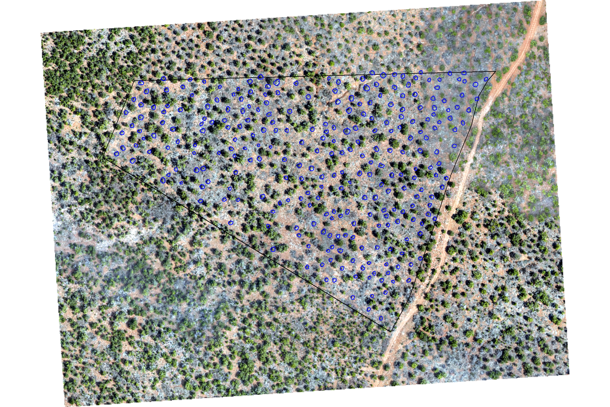
terra::res(pj_rgb_rast)## [1] 0.08 0.08plot RGB with the ground-truth piles (blue)
terra::plotRGB(pj_rgb_rast, stretch="lin")
terra::plot(
  pj_stand_boundary %>%
    terra::vect() %>%
    terra::project(terra::crs(pj_rgb_rast))
  , add = T, border = "black", col = NA, lwd = 1.2
)
terra::plot(
  pj_slash_piles_polys %>%
    terra::vect() %>%
    terra::project(terra::crs(pj_rgb_rast))
  , add = T, border = "blue", col = NA, lwd = 1.2
)
read crop point cloud
###############################################################
# read/crop point cloud
###############################################################
# output dir for clipped las
las_dir_temp <- "../data/Dawson_Data/point_cloud"
if(!dir.exists(las_dir_temp)){dir.create(las_dir_temp, showWarnings = F)}
# do it if not already done
if(dplyr::coalesce(length(list.files(las_dir_temp)),0)<1){
  # this reads the metadata from all files in the folder, not the points themselves.
  las_ctg <- lidR::readLAScatalog("d:/BLM_CO_SWDF_DawsonFuelsTreatment/Final/PointCloud/Tiles/")
  las_ctg
  # set ctg opts
  lidR::opt_select(las_ctg) <- "xyzainrcRGBNC"
  lidR::opt_progress(las_ctg) <- T
  # write generated results to disk storage rather than keeping everything in memory. This option can be activated with opt_output_files()
  lidR::opt_output_files(las_ctg) <- paste0(normalizePath(las_dir_temp),"/", "_{XLEFT}_{YBOTTOM}") # label outputs based on coordinates
  lidR::opt_filter(las_ctg) <- "-drop_duplicates"

  # clip the point cloud using the polygon and write to a new file
  # the lidR::opt_output_files is key to writing the output to disk without loading the entire clipped result into memory.
  clip_las_ctg <- lidR::clip_roi(
    las = las_ctg
    , geometry = pj_stand_boundary %>%
      sf::st_buffer(100) %>%
      sf::st_bbox() %>%
      sf::st_as_sfc() %>%
      sf::st_as_sf() %>%
      sf::st_transform(sf::st_crs(las_ctg))
  )
}else{
  clip_las_ctg <- lidR::readLAScatalog(las_dir_temp)
}
clip_las_ctg
## class : LAScatalog (v1.2 format 2)
## extent : 707813.6, 708409.9, 4193155, 4193638 (xmin, xmax, ymin, ymax)
## coord. ref. : NAD83(2011) / UTM zone 12N
## area : 288106.3 m²
## points : 163.84 million points
## type : terrestrial
## density : 568.7 points/m²
## density : 568.7 pulses/m²
## num. files : 1## [1] "../data/Dawson_Data/point_cloud/_707813.5_4193155.las"10.3 Process Raw Point Cloud
We’ll use cloud2trees::cloud2raster() to process the raw point cloud data
# output dir
c2t_output_dir <- "../data/Dawson_Data/"
dir_temp <- file.path(c2t_output_dir, "point_cloud_processing_delivery")
# do it
if(!dir.exists(dir_temp)){
# cloud2trees
cloud2raster_ans <- cloud2trees::cloud2raster(
output_dir = c2t_output_dir
, input_las_dir = las_dir_temp
, accuracy_level = 2
, keep_intrmdt = F
, dtm_res_m = 0.2
, chm_res_m = 0.1
, min_height = 0 # effectively generates a DSM based on non-ground points
)
}else{
dtm_temp <- terra::rast( file.path(dir_temp, "dtm_0.2m.tif") )
chm_temp <- terra::rast( file.path(dir_temp, paste0("chm_", 0.1,"m.tif")) )
cloud2raster_ans <- list(
"dtm_rast" = dtm_temp
, "chm_rast" = chm_temp
)
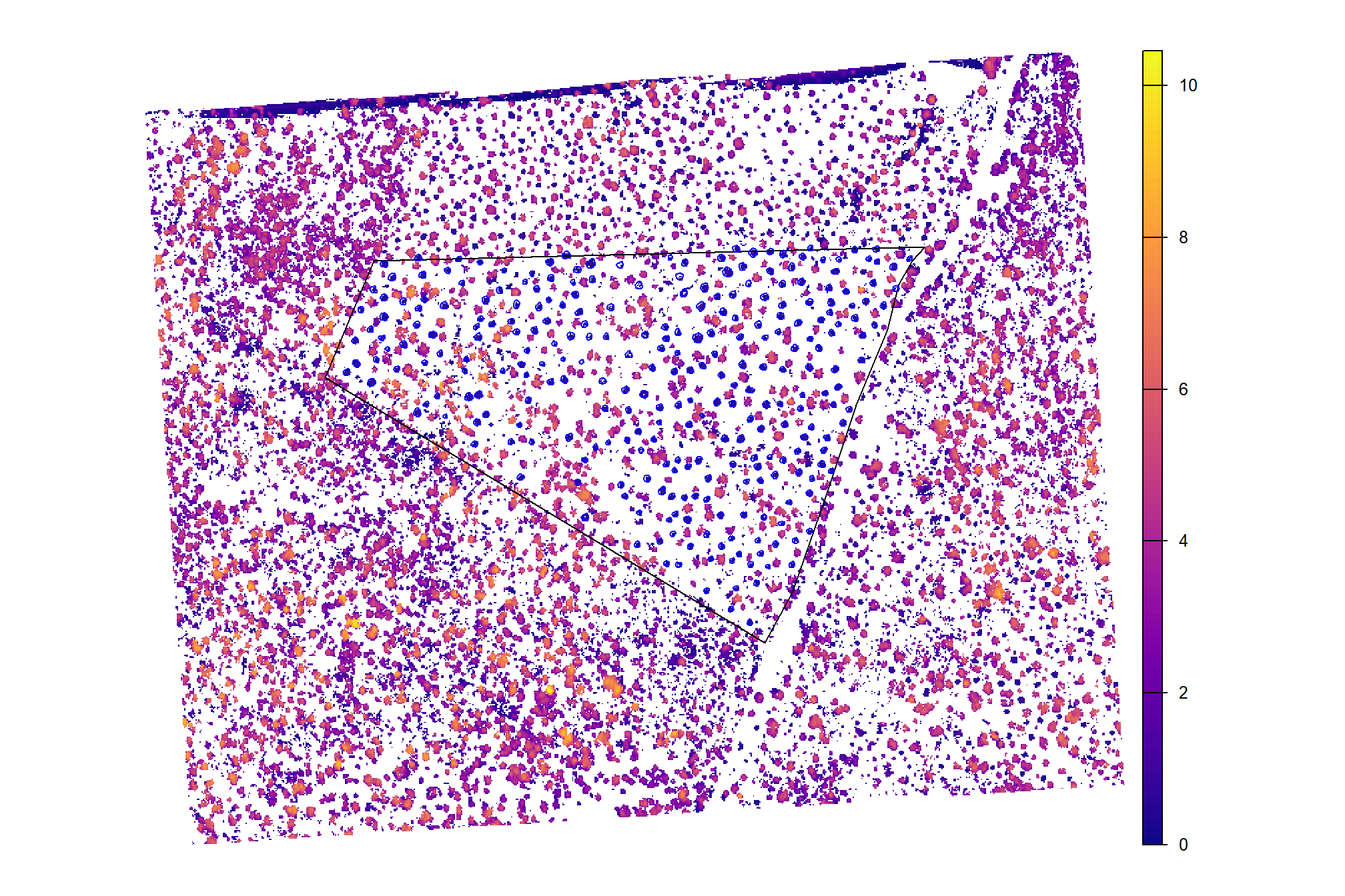
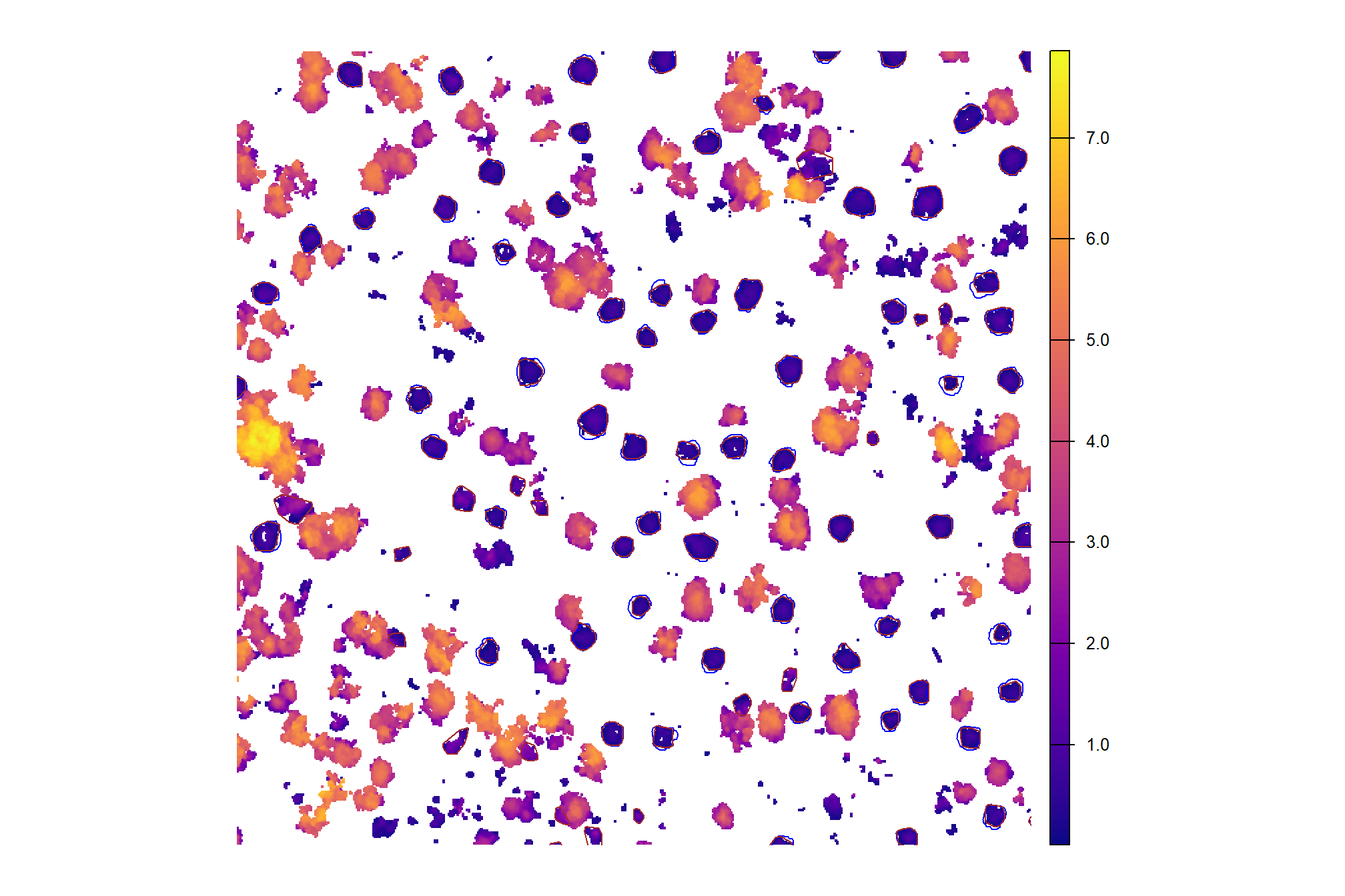
}plot CHM with the ground-truth piles (blue)
cloud2raster_ans$chm_rast %>%
  terra::aggregate(fact = 2, na.rm=T) %>%  #, fun = "median", cores = lasR::half_cores(), na.rm = T) %>%
  terra::plot(col = viridis::plasma(100), axes = F)
terra::plot(
  pj_stand_boundary %>%
    terra::vect() %>%
    terra::project(terra::crs(cloud2raster_ans$chm_rast))
  , add = T, border = "black", col = NA, lwd = 1.2
)
terra::plot(
  pj_slash_piles_polys %>%
    terra::vect() %>%
    terra::project(terra::crs(cloud2raster_ans$chm_rast))
  , add = T, border = "blue", col = NA, lwd = 1.2
)
plot DTM with the ground-truth piles (blue)
cloud2raster_ans$dtm_rast %>%
  terra::aggregate(fact = 2, na.rm=T) %>%  #, fun = "median", cores = lasR::half_cores(), na.rm = T) %>%
  terra::plot(col = harrypotter::hp(option = "mischief", n = 100, direction = -1), axes = F)
terra::plot(
  pj_stand_boundary %>%
    terra::vect() %>%
    terra::project(terra::crs(cloud2raster_ans$chm_rast))
  , add = T, border = "black", col = NA, lwd = 1.2
)
terra::plot(
  pj_slash_piles_polys %>%
    terra::vect() %>%
    terra::project(terra::crs(cloud2raster_ans$chm_rast))
  , add = T, border = "blue", col = NA, lwd = 1.2
)
10.4 Pile Detection: Data Fusion
since we have both structural and spectral data, we’ll start by using the data fusion approach and do a full walk-through of our detection results after which we’ll circle back to explore results obtained using structural data only.
we’ll work with the CHM in the study unit boundary plus a buffer to limit the amount of data we process
chm_rast_stand <- cloud2raster_ans$chm_rast %>%
  terra::crop(
    pj_stand_boundary %>%
      sf::st_buffer(10) %>%
      terra::vect() %>%
      terra::project(terra::crs(cloud2raster_ans$chm_rast))
  ) %>%
  terra::mask(
    pj_stand_boundary %>%
      sf::st_buffer(10) %>%
      terra::vect() %>%
      terra::project(terra::crs(cloud2raster_ans$chm_rast))
  )
# # huh?
# chm_rast_stand %>%
#   terra::aggregate(fact = 2, na.rm=T) %>%  #, fun = "median", cores = lasR::half_cores(), na.rm = T) %>%
#   terra::plot(col = viridis::plasma(100), axes = F)
#   terra::plot(
#     pj_stand_boundary %>%
#       terra::vect() %>%
#       terra::project(terra::crs(cloud2raster_ans$chm_rast))
#     , add = T, border = "black", col = NA, lwd = 1.2
#   )
#   terra::plot(
#     pj_slash_piles_polys %>%
#       terra::vect() %>%
#       terra::project(terra::crs(cloud2raster_ans$chm_rast))
#     , add = T, border = "blue", col = NA, lwd = 1.2
#   )
10.4.1 Structural Candidate Segments
we’ll start by detecting candidate slash piles based on the structural CHM data alone with our slash_pile_detect_watershed() function we defined in this earlier section.
we’re going to set the four structural parameters (max_ht_m, max_area_m2, convexity_pct, circle_fit_iou_pct) which are used to determine candidate slash piles from the CHM data alone based on our expectations from the treatment prescription and it’s implementation on the ground.
the treatment prescription for the unit of interest called for thinning to create a residual structure with “uniform gaps between trees” with via a “heavy intensity thinning” that called for gaps of “at least 30 feet between tree crowns” with “70% of the retained (i.e. leave) trees should be over 8 inches basal diameter if present and 30% should be between 2 inches and 8 inches in basal diameter.” Here is the exact wording of the slash pile construction prescription:
No less than 90% of all cut trees, live limbs and slash shall be piled. Piles are to be constructed to facilitate burning by the government at a later date. Minimum pile size is 5x5x5 feet. The contractor shall construct piles that are sufficiently compacted to allow for a high percentage of consumption from burning, this may require multiple cutting of stems, compacting the pile with equipment or other approved techniques. Piles should be constructed with branches and smaller diameter fuels piled on bottom and larger limbs/bole wood piled on top. Piles should be spaced appropriately away from leave trees to avoid damage from burning. Anticipate flame lengths twice the piled fuel height when placing piles i.e (5 ft tall pile will have 10 ft flame lengths so pile should be placed at least 10 ft away from the nearest reserve trees). Piles will be constructed in a way to prevent toppling. Piles may be placed on stumps. Oak and other brush cut will need to be added to the piles. Piles shall not be constructed in swales, streams, springs, or within 15 feet any recreational trail within the units. Piles shall not be placed on or near any cadastral survey markers. Piles may not be built under any electrical transmission line or utility line. Piles shall be free of soil.
Site managers also provided anecdotal feedback about the on-the-ground prescription implementation, noting that the piles were “larger than expected” and “messy,” and were constructed too close to residual trees. The prescription specified a minimum pile size of 1.5 meters (5 feet) long, wide, and tall, but provided no explicit maximum size. This absence of a maximum size makes the anecdotal feedback particularly relevant for setting up our pile detection methodology. The close proximity of piles to trees, which resulted in tree mortality on other units when piles were burned, may also complicate our detection methodology, as the structural and spectral signatures of the piles and trees may merge in both the CHM and RGB raster data.
We also have the benefit of using spectral data to further filter the candidate piles detected from the structural data. This allows us to set less restrictive structural parameters which will increase the number of structurally-detected piles. To compensate for this less restrictive filtering on the structural side, we will set the spectral_weight parameter to ‘4’, which applies four of the five thresholds and represents the optimal spectral filtering identified in by the training data set. This reliance on the spectral data helps to filter out false positives that may be shrubs, lower tree branches, or boulders.
Based on the prescription and anecdotal feedback, the following parameter settings will be used:
- max_ht_m: This parameter will be set to 2.0 m (6.5 feet). This represents a 33% increase over the 1.5 m (5 ft) minimum height specified in the prescription, to account for the feedback that piles were larger than expected.
- min_ht_m: This parameter will be set to 0.3 m (1.0 foot). This creates a large 1.7 m (5.6 feet) vertical range for structural detection. This setting allows for the acceptance of piles up to 1.2 m (4.0 feet) smaller than the prescribed minimum of 1.5 m but this low threshold will be offset by the subsequent strict spectral filtering
- min_area_m2: This parameter will be set to 2.0 square meters (21.5 square feet). This provides a small buffer below the prescribed 2.3 square meters (25 square feet) minimum area to account for minor segmentation errors or slight settling of the pile, without deviating significantly from the horizontal prescription.
- max_area_m2: This parameter will be set to 17 square meters (183 square feet). This represents a nearly eight-fold increase compared to the 2.3 square meters minimum. The rationale for this significant increase compared to the upper height threshold is because it is physically easier to construct piles that are wider and more irregular in the horizontal direction than the vertical direction
- convexity_pct: To account for the “messy” and irregularly shaped piles, this parameter will be set to 0.08 which is in the the optimal range identified in the Ponderosa Pine training data. This less restrictive threshold will allow for the structural detection of more irregular pile footprints
- circle_fit_iou_pct: This parameter will be set to 0.32, which is approximately 12 percentage points lower than the optimal value identified in the Ponderosa Pine training data. This value is used in conjunction with convexity_pct to allow for a wider range of non-circular, irregular shapes
- CHM Resolution (chm_res_m): A 0.1 m (0.33 feet; 3.9 inches) CHM raster will be used. This fine resolution will enhance the granular distinction between piles and lower tree branches which is important given the close proximity of piles to residual trees noted by managers
slash_pile_detect_watershed() that CHM
outdir_temp <- "../data/Dawson_data"
fnm_temp <- file.path(outdir_temp,"pj_structural_candidate_segments.gpkg")
# "new_pj_structural_candidate_segments.gpkg" = convexity_pct = 0.06; circle_fit_iou_pct = 0.35
if(!file.exists(fnm_temp)){
  set.seed(111)
  slash_pile_detect_watershed_ans <- slash_pile_detect_watershed(
    chm_rast = chm_rast_stand
    #### height and area thresholds for the detected piles
    # these should be based on data from the literature or expectations based on the prescription
    , max_ht_m = 2.3 # set the max expected pile height
    , min_ht_m = 0.3 # set the min expected pile height
    , min_area_m2 = 2.0 # set the min expected pile area
    , max_area_m2 = 17 # set the max expected pile area
    #### irregularity filtering
    # 1 = perfectly convex (no inward angles); 0 = so many inward angles
    # values closer to 1 remove more irregular segments;
      # values closer to 0 keep more irregular segments (and also regular segments)
    # these will all be further filtered for their circularity and later smoothed to remove blocky edges
    # and most inward angles by applying a convex hull to the original detected segment
    , convexity_pct = 0.08 # min required overlap between the predicted pile and the convex hull of the predicted pile
    #### circularity filtering
    # 1 = perfectly circular; 0 = not circular (e.g. linear) but also circular
    # min required IoU between the predicted pile and the best fit circle of the predicted pile
    , circle_fit_iou_pct = 0.30
    #### shape refinement & overlap removal
    ## smooth_segs = T ... convex hulls of raster detected segments are returned, any that overlap are removed
    ## smooth_segs = F ... raster detected segments are returned (blocky) if they meet all prior rules
    , smooth_segs = T
  )
  # save
  slash_pile_detect_watershed_ans %>% sf::st_write(fnm_temp, append = F)
}else{
  slash_pile_detect_watershed_ans <- sf::st_read(fnm_temp, quiet=T)
}
# what did we get?
slash_pile_detect_watershed_ans %>% dplyr::glimpse()
## Rows: 397
## Columns: 8
## $ pred_id <int> 1, 5, 7, 9, 10, 11, 12, 13, 14, 15, 16, 18, 20, 21, 24…
## $ area_m2 <dbl> 12.410, 9.145, 16.630, 9.715, 8.560, 2.820, 9.775, 4.1…
## $ volume_m3 <dbl> 7.611119, 11.283464, 18.274028, 16.730727, 11.332464, …
## $ max_height_m <dbl> 1.500000, 2.300000, 2.290000, 2.300000, 2.300000, 2.30…
## $ volume_per_area <dbl> 0.6133054, 1.2338397, 1.0988592, 1.7221541, 1.3238860,…
## $ pct_chull <dbl> 0.7687349, 0.6790596, 0.7257968, 0.5795162, 0.6810748,…
## $ diameter_m <dbl> 5.223983, 5.292447, 5.554278, 4.272002, 4.565085, 2.64…
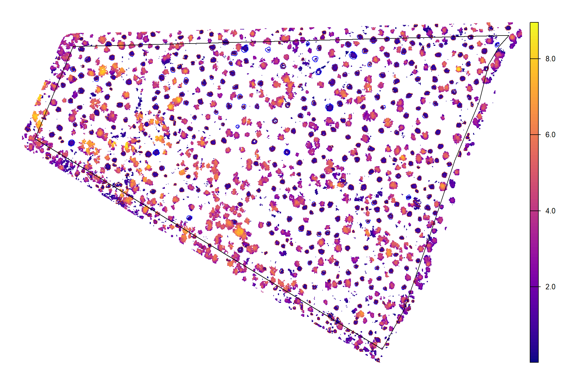
## $ geom <POLYGON [m]> POLYGON ((707989.7 4193402,..., POLYGON ((7081…CHM with the predicted piles (brown) and the ground-truth piles (blue)
chm_rast_stand %>%
  terra::aggregate(fact = 2, na.rm=T) %>%  #, fun = "median", cores = lasR::half_cores(), na.rm = T) %>%
  terra::plot(col = viridis::plasma(100), axes = F)
  terra::plot(
    pj_stand_boundary %>%
      terra::vect() %>%
      terra::project(terra::crs(cloud2raster_ans$chm_rast))
    , add = T, border = "black", col = NA, lwd = 1.2
  )
  terra::plot(
    pj_slash_piles_polys %>%
      terra::vect() %>%
      terra::project(terra::crs(cloud2raster_ans$chm_rast))
    , add = T, border = "blue", col = NA, lwd = 1.2
  )
  terra::plot(
    slash_pile_detect_watershed_ans %>%
      terra::vect() %>%
      terra::project(terra::crs(cloud2raster_ans$chm_rast))
    , add = T, border = "brown", col = NA, lwd = 1.3
  )
we can also use mapview::mapview() to interactively plot the CHM with the predicted piles (brown) and the ground-truth piles (blue)
chm_rast_stand %>%
  terra::aggregate(fact = 2, na.rm=T) %>%  #, fun = "median", cores = lasR::half_cores(), na.rm = T) %>%
  mapview::mapview() +
  mapview::mapview(
    pj_stand_boundary
    , alpha.regions = 0, color = "black", lwd = 1
    , legend=F,label=F,popup=F
  ) +
  mapview::mapview(
    pj_slash_piles_polys
    , alpha.regions = 0, color = "blue", lwd = 1.2
    , legend=F,label=F
  ) +
  mapview::mapview(
    slash_pile_detect_watershed_ans
    , alpha.regions = 0, color = "brown", lwd = 1.3
    , legend=F,label=F
  )
## |---------|---------|---------|---------|========================================= let’s focus in on a specific area to plot the ground truth and the predicted piles overlaid on the RGB.
aoi_for_plt <-
  pj_slash_piles_polys %>%
  dplyr::filter(pile_id == 210) %>%
  sf::st_as_sfc() %>%
  sf::st_transform(sf::st_crs(slash_pile_detect_watershed_ans)) %>%
  sf::st_buffer(55) %>%
  sf::st_bbox() %>%
  sf::st_as_sfc() %>%
  sf::st_as_sf()
# all gt piles that intersect
gt_temp <- pj_slash_piles_polys %>%
  dplyr::inner_join(
    pj_slash_piles_polys %>%
      sf::st_transform(sf::st_crs(aoi_for_plt)) %>%
      sf::st_intersection(aoi_for_plt) %>%
      sf::st_drop_geometry() %>%
      dplyr::select(pile_id)
  ) %>%
  sf::st_transform(sf::st_crs(aoi_for_plt))
# all pred piles that intersect
pred_temp <- slash_pile_detect_watershed_ans %>%
  dplyr::inner_join(
    slash_pile_detect_watershed_ans %>%
      sf::st_intersection(aoi_for_plt) %>%
      sf::st_drop_geometry() %>%
      dplyr::select(pred_id)
  )
# plot it
ortho_plt_temp <-
  ortho_plt_fn(
    my_ortho_rast = pj_rgb_rast
    , stand = aoi_for_plt
    , buffer = 5
  )
# ortho_plt_temp
plot a sample of the RGB with the predicted piles (brown) and the ground-truth piles (blue)
ortho_plt_temp +
  # ggplot2::ggplot() +
  ggplot2::geom_sf(
    data = gt_temp
    , color = "blue"
    , fill = NA
    , lwd = 1
  ) +
  ggplot2::geom_sf(
    data = pred_temp
    , color = "brown"
    , fill = NA
    , lwd = 1
  ) +
  ggplot2::theme_void() +
  ggplot2::theme(legend.position = "none")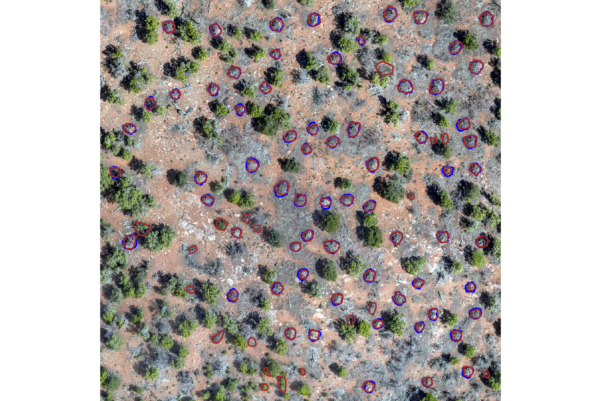
plot the same sample of the CHM with the predicted piles (brown) and the ground-truth piles (blue)
cloud2raster_ans$chm_rast %>%
  terra::crop(aoi_for_plt %>% terra::vect() %>% terra::project(cloud2raster_ans$chm_rast)) %>%
  terra::mask(aoi_for_plt %>% terra::vect() %>% terra::project(cloud2raster_ans$chm_rast)) %>%
  terra::aggregate(fact = 2, na.rm=T) %>%  #, fun = "median", cores = lasR::half_cores(), na.rm = T) %>%
  terra::plot(col = viridis::plasma(100), axes = F)
  terra::plot(
    gt_temp %>%
      terra::vect() %>%
      terra::project(terra::crs(cloud2raster_ans$chm_rast))
    , add = T, border = "blue", col = NA, lwd = 1.2
  )
  terra::plot(
    pred_temp %>%
      terra::vect() %>%
      terra::project(terra::crs(cloud2raster_ans$chm_rast))
    , add = T, border = "brown", col = NA, lwd = 1.3
  )
10.4.2 Accuracy of these spectral settings
let’s quickly look at the accuracy of the pile detection if we were to only use the structural data to identify piles with these specific settings.
note, that if we only had structural data, we would be much more restrictive in setting the pile detection parameters as we’ll demonstrate below.
we aren’t going to fully discuss this accuracy assessment, it is presented only for the curious
# add filter for those in stand
# pred
struct_temp <- slash_pile_detect_watershed_ans %>%
  dplyr::left_join(
    slash_pile_detect_watershed_ans %>%
      sf::st_intersection(
        pj_stand_boundary %>%
          sf::st_transform(sf::st_crs(slash_pile_detect_watershed_ans))
      ) %>%
      sf::st_drop_geometry() %>%
      dplyr::distinct(pred_id) %>%
      dplyr::mutate(is_in_stand=T)
    , by = "pred_id"
  ) %>%
  dplyr::mutate(is_in_stand=dplyr::coalesce(is_in_stand, F))
# ground truth and prediction matching process
gt_pred_match_temp <- ground_truth_prediction_match(
  ground_truth =
    pj_slash_piles_polys %>%
    dplyr::filter(is_in_stand) %>%
    dplyr::arrange(desc(field_diameter_m)) %>%
    sf::st_transform(sf::st_crs(struct_temp))
  , gt_id = "pile_id"
  , predictions = struct_temp %>% dplyr::filter(is_in_stand)
  , pred_id = "pred_id"
  , min_iou_pct = 0.05
)
# add data from gt and pred piles
gt_pred_match_temp <-
  gt_pred_match_temp %>%
  # add area of gt
  dplyr::left_join(
    pj_slash_piles_polys %>%
      sf::st_drop_geometry() %>%
      dplyr::filter(is_in_stand) %>%
      dplyr::select(
        pile_id
        , image_gt_area_m2
        , image_gt_diameter_m
        , field_gt_volume_m3
        , height_m
        , field_diameter_m
      ) %>%
      dplyr::rename(
        gt_height_m = height_m
        , gt_diameter_m = field_diameter_m
        , gt_area_m2 = image_gt_area_m2
        , gt_volume_m3 = field_gt_volume_m3
      ) %>%
      dplyr::mutate(pile_id=as.numeric(pile_id))
    , by = "pile_id"
  ) %>%
  # add info from predictions
  dplyr::left_join(
    struct_temp %>%
      sf::st_drop_geometry() %>%
      dplyr::select(
        pred_id
        , area_m2, volume_m3, max_height_m, diameter_m
      ) %>%
      dplyr::rename(
        pred_area_m2 = area_m2, pred_volume_m3 = volume_m3
        , pred_height_m = max_height_m, pred_diameter_m = diameter_m
      )
    , by = dplyr::join_by(pred_id)
  ) %>%
  dplyr::mutate(
    ### calculate these based on the formulas below...agg_ground_truth_match() depends on those formulas
    # ht diffs
    diff_height_m = pred_height_m-gt_height_m
    , pct_diff_height_m = (gt_height_m-pred_height_m)/gt_height_m
    # diameter
    , diff_field_diameter_m = pred_diameter_m-gt_diameter_m
    , pct_diff_field_diameter_m = (gt_diameter_m-pred_diameter_m)/gt_diameter_m
    # image diameter
    , diff_image_diameter_m = pred_diameter_m-image_gt_diameter_m
    , pct_diff_image_diameter_m = (image_gt_diameter_m-pred_diameter_m)/image_gt_diameter_m
    # area diffs
    , diff_area_m2 = pred_area_m2-gt_area_m2
    , pct_diff_area_m2 = (gt_area_m2-pred_area_m2)/gt_area_m2
    # # volume diffs
    # , diff_image_volume_m3 = pred_volume_m3-image_gt_volume_m3
    # , pct_diff_image_volume_m3 = (image_gt_volume_m3-pred_volume_m3)/image_gt_volume_m3
    # , diff_field_volume_m3 = pred_volume_m3-field_gt_volume_m3
    # , pct_diff_field_volume_m3 = (field_gt_volume_m3-pred_volume_m3)/field_gt_volume_m3
  )
# huh?
agg_ground_truth_match(ground_truth_prediction_match_ans = gt_pred_match_temp) %>%
kbl_agg_gt_match(caption = "pile detection and form quantification accuracy metrics<br>structural only prior to data fusion")| . | value | |
|---|---|---|
| Detection Count | TP | 262 |
| FN | 15 | |
| FP | 79 | |
| Detection | F-score | 85% |
| Recall | 95% | |
| Precision | 77% | |
| Area m2 | ME | -1.19 |
| RMSE | 2.0 | |
| MAPE | 15% | |
| Diameter m (field) | ME | -1.71 |
| RMSE | 1.8 | |
| MAPE | 31% | |
| Diameter m (image) | ME | -0.26 |
| RMSE | 0.5 | |
| MAPE | 8% | |
| Height m | ME | -1.17 |
| RMSE | 1.2 | |
| MAPE | 51% |
10.4.3 Spectral Filtering of Candidate Segments
Now we’ll filter the structurally-detected candidate slash piles using the RGB spectral data with the polygon_spectral_filtering() function we defined in this earlier section
The spectral filtering approach is a data fusion method used to filter candidate slash pile detections first identified using structural data alone. After initial candidates are identified based on structural data, this method applies a set of five spectral index thresholds to the candidate segments. The spectral_weight parameter is an integer from 1 to 5 that directly controls the number of thresholds that are applied. For example, a value of “3” means a candidate pile must pass at least three of the five thresholds to be retained. This process helps to filter out objects like shrubs, lower tree branches, or boulders that may have been structurally misidentified as piles.
we will set the spectral_weight parameter to ‘4’, which applies four of the five thresholds and represents the optimal spectral filtering identified in by the training data set. This reliance on the spectral data helps to filter out false positives that may be shrubs, lower tree branches, or boulders.
final_predicted_slash_piles <- polygon_spectral_filtering(
  sf_data = slash_pile_detect_watershed_ans
  , rgb_rast = pj_rgb_rast
  # define the band index
  , red_band_idx = 1
  , green_band_idx = 2
  , blue_band_idx = 3
  # spectral weighting
  , spectral_weight = 4
)
what did we get?
## Rows: 397
## Columns: 23
## $ pred_id          <int> 1, 5, 7, 9, 10, 11, 12, 13, 14, 15, 16, 18, 20, 21, 2…
## $ area_m2          <dbl> 12.410, 9.145, 16.630, 9.715, 8.560, 2.820, 9.775, 4.…
## $ volume_m3        <dbl> 7.611119, 11.283464, 18.274028, 16.730727, 11.332464,…
## $ max_height_m     <dbl> 1.500000, 2.300000, 2.290000, 2.300000, 2.300000, 2.3…
## $ volume_per_area  <dbl> 0.6133054, 1.2338397, 1.0988592, 1.7221541, 1.3238860…
## $ pct_chull        <dbl> 0.7687349, 0.6790596, 0.7257968, 0.5795162, 0.6810748…
## $ diameter_m       <dbl> 5.223983, 5.292447, 5.554278, 4.272002, 4.565085, 2.6…
## $ rast_agg_grvi    <dbl> -0.0242606787, -0.0046708129, -0.0325958568, -0.01224…
## $ rast_agg_rgri    <dbl> 1.0497278, 1.0093855, 1.0673883, 1.0247954, 1.0838725…
## $ rast_agg_vdvi    <dbl> -0.003656942, 0.039179734, -0.010469513, 0.023582234,…
## $ rast_agg_rgbvi   <dbl> -0.006476210, 0.083397656, -0.019700427, 0.049979234,…
## $ rast_agg_exg     <dbl> -0.004869986, 0.052930918, -0.013910804, 0.031692102,…
## $ rast_agg_exr     <dbl> 0.1556979, 0.1459419, 0.1625862, 0.1491834, 0.1692692…
## $ rast_agg_exgr    <dbl> -0.160947212, -0.093805306, -0.176345140, -0.11713800…
## $ rast_agg_bi      <dbl> 0.4539163, 0.4429114, 0.4957423, 0.4909618, 0.4905459…
## $ rast_agg_sat     <dbl> 0.08239188, 0.17601331, 0.08864828, 0.16517131, 0.100…
## $ geom             <POLYGON [m]> POLYGON ((707989.7 4193402,..., POLYGON ((708…
## $ inrange_th_exgr  <dbl> 1, 1, 1, 1, 1, 1, 1, 1, 1, 1, 1, 1, 1, 1, 1, 1, 1, 1,…
## $ inrange_th_rgri  <dbl> 1, 1, 1, 1, 1, 1, 1, 1, 1, 1, 1, 1, 1, 1, 1, 1, 1, 1,…
## $ inrange_th_vdvi  <dbl> 1, 0, 1, 1, 1, 1, 1, 0, 1, 1, 1, 1, 1, 0, 1, 0, 0, 0,…
## $ inrange_th_bi    <dbl> 1, 1, 1, 1, 1, 1, 1, 1, 1, 1, 1, 1, 1, 1, 1, 1, 1, 1,…
## $ inrange_th_sat   <dbl> 1, 1, 1, 1, 1, 1, 1, 1, 1, 1, 1, 0, 1, 1, 0, 1, 1, 1,…
## $ inrange_th_votes <dbl> 5, 4, 5, 5, 5, 5, 5, 4, 5, 5, 5, 4, 5, 4, 4, 4, 4, 4,…how many piles were removed?
# how many piles were removed?
nrow(slash_pile_detect_watershed_ans)-nrow(final_predicted_slash_piles)
## [1] 0# what proportion were removed?
scales::percent(
(nrow(slash_pile_detect_watershed_ans)-nrow(final_predicted_slash_piles))/nrow(slash_pile_detect_watershed_ans)
, accuracy=0.1
)## [1] "0.0%"The outcome of 0 candidate piles removed by the spectral filter, despite requiring at least four of the five spectral index thresholds be met, is a surprising result. This indicates that integrating spectral data did not alter the final retained pile count compared to the structural-only detection, even though the spectral component is designed specifically to reduce False Positive (FP) predictions.
This finding suggests that the detection method using structural data alone would achieve a similar overall accuracy to the data fusion approach. This result is attributable to the specific spectral signatures at this site, leading to the spectral filter’s ineffectiveness (see primary possibilities below). We intentionally set less restrictive structural (min_ht_m, max_ht_m, min_area_m2, and max_area_m2) and geometric (circle_fit_iou_pct, convexity_pct) parameters for this validation, anticipating that the spectral data would successfully compensate for this looser structural filtering—a compensation that did not actualize here. In practice, if spectral data were truly unavailable, we would recommend setting these structural and geometric parameters more strictly.
The unexpected outcome suggests two primary possibilities for the filter’s failure to remove incorrect pile predictions:
- Minimal Spectral Difference between Piles and False Positives (FPs): The spectral signatures of the actual True Positive (TP) piles and the structurally detected FPs are likely too similar. For instance, many FPs might be senescent vegetation (dead shrubs or short trees lacking greenness) whose spectral appearance closely mimics the dead wood expected in slash piles. The similar signatures occur even though three of the five thresholds target the removal of healthy, green vegetation.
- Insufficient Sensitivity of Spectral Thresholds: The spectral index thresholds themselves may lack the sensitivity needed to differentiate vegetation in this arid environment. The native vegetation here may naturally exhibit lower greenness than the typical healthy vegetation used to define the thresholds in the source studies (Wang et al. 2025; Riehle et al. 2020).
10.4.3.1 Maximum spectral filtering
Given this lack of impact, we will test increasing the spectral_weight parameter to ‘5’ which is the maximum possible strictness requiring all five spectral index thresholds to be met. While statistical analysis on the Ponderosa Pine training data showed similar overall detection accuracies between a setting of ‘4’ and ‘5’, this maximum setting presents an increased risk of removing True Positive piles that have atypical spectral signatures. Such atypical signatures could result from piles that are heavily sun-bleached (appearing bright white spectrally) or those that are in the shadow of surrounding canopy at the time of image capture (appearing very dark).
we aren’t going to fully discuss this accuracy assessment, it is presented only for the curious
polygon_spectral_filtering_temp <- polygon_spectral_filtering(
  sf_data = slash_pile_detect_watershed_ans
  , rgb_rast = pj_rgb_rast
  # define the band index
  , red_band_idx = 1
  , green_band_idx = 2
  , blue_band_idx = 3
  # spectral weighting
  , spectral_weight = 5
)
# add filter for those in stand
# pred
struct_temp <- polygon_spectral_filtering_temp %>%
  dplyr::left_join(
    polygon_spectral_filtering_temp %>%
      sf::st_intersection(
        pj_stand_boundary %>%
          sf::st_transform(sf::st_crs(polygon_spectral_filtering_temp))
      ) %>%
      sf::st_drop_geometry() %>%
      dplyr::distinct(pred_id) %>%
      dplyr::mutate(is_in_stand=T)
    , by = "pred_id"
  ) %>%
  dplyr::mutate(is_in_stand=dplyr::coalesce(is_in_stand, F))
# ground truth and prediction matching process
gt_pred_match_temp <- ground_truth_prediction_match(
  ground_truth =
    pj_slash_piles_polys %>%
    dplyr::filter(is_in_stand) %>%
    dplyr::arrange(desc(field_diameter_m)) %>%
    sf::st_transform(sf::st_crs(struct_temp))
  , gt_id = "pile_id"
  , predictions = struct_temp %>% dplyr::filter(is_in_stand)
  , pred_id = "pred_id"
  , min_iou_pct = 0.05
)
# add data from gt and pred piles
gt_pred_match_temp <-
  gt_pred_match_temp %>%
  # add area of gt
  dplyr::left_join(
    pj_slash_piles_polys %>%
      sf::st_drop_geometry() %>%
      dplyr::filter(is_in_stand) %>%
      dplyr::select(
        pile_id
        , image_gt_area_m2
        , image_gt_diameter_m
        , field_gt_volume_m3
        , height_m
        , field_diameter_m
      ) %>%
      dplyr::rename(
        gt_height_m = height_m
        , gt_diameter_m = field_diameter_m
        , gt_area_m2 = image_gt_area_m2
        , gt_volume_m3 = field_gt_volume_m3
      ) %>%
      dplyr::mutate(pile_id=as.numeric(pile_id))
    , by = "pile_id"
  ) %>%
  # add info from predictions
  dplyr::left_join(
    struct_temp %>%
      sf::st_drop_geometry() %>%
      dplyr::select(
        pred_id
        , area_m2, volume_m3, max_height_m, diameter_m
      ) %>%
      dplyr::rename(
        pred_area_m2 = area_m2, pred_volume_m3 = volume_m3
        , pred_height_m = max_height_m, pred_diameter_m = diameter_m
      )
    , by = dplyr::join_by(pred_id)
  ) %>%
  dplyr::mutate(
    ### calculate these based on the formulas below...agg_ground_truth_match() depends on those formulas
    # ht diffs
    diff_height_m = pred_height_m-gt_height_m
    , pct_diff_height_m = (gt_height_m-pred_height_m)/gt_height_m
    # diameter
    , diff_field_diameter_m = pred_diameter_m-gt_diameter_m
    , pct_diff_field_diameter_m = (gt_diameter_m-pred_diameter_m)/gt_diameter_m
    # image diameter
    , diff_image_diameter_m = pred_diameter_m-image_gt_diameter_m
    , pct_diff_image_diameter_m = (image_gt_diameter_m-pred_diameter_m)/image_gt_diameter_m
    # area diffs
    , diff_area_m2 = pred_area_m2-gt_area_m2
    , pct_diff_area_m2 = (gt_area_m2-pred_area_m2)/gt_area_m2
    # # volume diffs
    # , diff_image_volume_m3 = pred_volume_m3-image_gt_volume_m3
    # , pct_diff_image_volume_m3 = (image_gt_volume_m3-pred_volume_m3)/image_gt_volume_m3
    # , diff_field_volume_m3 = pred_volume_m3-field_gt_volume_m3
    # , pct_diff_field_volume_m3 = (field_gt_volume_m3-pred_volume_m3)/field_gt_volume_m3
  )
# huh?
agg_ground_truth_match(ground_truth_prediction_match_ans = gt_pred_match_temp) %>%
  kbl_agg_gt_match(caption = "pile detection and form quantification accuracy metrics<br>exploration data fusion `spectral_weight` set to '5'")
we can compare this to the detection and quantification accuracy results of the spectral_weight parameter set to ‘4’ which is what we will present in the manuscript of this project
10.4.4 Detection and Quantification Accuracy
let’s see how we did given the list of predictions compared to the ground truth data using the confusion matrix matching process we outlined in this earlier section.
we’ll filter both ground truth and predicted piles to keep only those that actually intersect with the study unit boundary for comparison
# add filter
# pred
final_predicted_slash_piles <- final_predicted_slash_piles %>%
  dplyr::left_join(
    final_predicted_slash_piles %>%
      sf::st_intersection(
        pj_stand_boundary %>%
          sf::st_transform(sf::st_crs(final_predicted_slash_piles))
      ) %>%
      sf::st_drop_geometry() %>%
      dplyr::distinct(pred_id) %>%
      dplyr::mutate(is_in_stand=T)
    , by = "pred_id"
  ) %>%
  dplyr::mutate(is_in_stand=dplyr::coalesce(is_in_stand, F))
10.4.4.1 Instance matching
now apply the instance matching process we outlined in this earlier section to establish True Positives (TP), False Positives (FP, commissions), and False Negatives (FN, omissions)
# ground truth and prediction matching process
ground_truth_prediction_match_ans <- ground_truth_prediction_match(
  ground_truth =
    pj_slash_piles_polys %>%
    dplyr::filter(is_in_stand) %>%
    dplyr::arrange(desc(field_diameter_m)) %>%
    sf::st_transform(sf::st_crs(final_predicted_slash_piles))
  , gt_id = "pile_id"
  , predictions = final_predicted_slash_piles %>% dplyr::filter(is_in_stand)
  , pred_id = "pred_id"
  , min_iou_pct = 0.05
)
# add data from gt and pred piles
ground_truth_prediction_match_ans <-
  ground_truth_prediction_match_ans %>%
  # add area of gt
  dplyr::left_join(
    pj_slash_piles_polys %>%
      sf::st_drop_geometry() %>%
      dplyr::filter(is_in_stand) %>%
      dplyr::select(
        pile_id
        , image_gt_area_m2
        , image_gt_diameter_m
        , field_gt_volume_m3
        , height_m
        , field_diameter_m
      ) %>%
      dplyr::rename(
        gt_height_m = height_m
        , gt_diameter_m = field_diameter_m
        , gt_area_m2 = image_gt_area_m2
        , gt_volume_m3 = field_gt_volume_m3
      ) %>%
      dplyr::mutate(pile_id=as.numeric(pile_id))
    , by = "pile_id"
  ) %>%
  # add info from predictions
  dplyr::left_join(
    slash_pile_detect_watershed_ans %>%
      sf::st_drop_geometry() %>%
      dplyr::select(
        pred_id
        , area_m2, volume_m3, max_height_m, diameter_m
      ) %>%
      dplyr::rename(
        pred_area_m2 = area_m2, pred_volume_m3 = volume_m3
        , pred_height_m = max_height_m, pred_diameter_m = diameter_m
      )
    , by = dplyr::join_by(pred_id)
  ) %>%
  dplyr::mutate(
    ### calculate these based on the formulas below...agg_ground_truth_match() depends on those formulas
    # ht diffs
    diff_height_m = pred_height_m-gt_height_m
    , pct_diff_height_m = (gt_height_m-pred_height_m)/gt_height_m
    # diameter
    , diff_field_diameter_m = pred_diameter_m-gt_diameter_m
    , pct_diff_field_diameter_m = (gt_diameter_m-pred_diameter_m)/gt_diameter_m
    # image diameter
    , diff_image_diameter_m = pred_diameter_m-image_gt_diameter_m
    , pct_diff_image_diameter_m = (image_gt_diameter_m-pred_diameter_m)/image_gt_diameter_m
    # area diffs
    , diff_area_m2 = pred_area_m2-gt_area_m2
    , pct_diff_area_m2 = (gt_area_m2-pred_area_m2)/gt_area_m2
    # # volume diffs
    # , diff_image_volume_m3 = pred_volume_m3-image_gt_volume_m3
    # , pct_diff_image_volume_m3 = (image_gt_volume_m3-pred_volume_m3)/image_gt_volume_m3
    # , diff_field_volume_m3 = pred_volume_m3-field_gt_volume_m3
    # , pct_diff_field_volume_m3 = (field_gt_volume_m3-pred_volume_m3)/field_gt_volume_m3
  )
# huh?
# ground_truth_prediction_match_ans %>% dplyr::glimpse()
that’s a lot of great detail at the individual pile instance level for us to dig into. before we do that, let’s aggregate the instances to see how we did at the stand level overall
10.4.4.2 Overall (stand level)
Now we’ll aggregate the instance matching results to calculate overall performance assessment metrics. Here, we take the counts of True Positives (TP), False Positives (FP, commissions), and False Negatives (FN, omissions), to determine overall accuracy. This aggregation will give us two types of results:
detection accuracy metrics: such as Recall, Precision, and F-score, are calculated directly by aggregating these raw TP, FP, and FN counts and quantifies the method’s ability to find the piles
quantification accuracy metrics: such as RMSE, MAPE, and Mean Error of pile form measurements (e.g. height, diameter) are calculated by aggregating the differences between the estimated pile attributes and the ground truth values for instances classified as True Positives. These metrics tell us about the method’s ability to accurately quantify the form of the piles it successfully identified
agg_ground_truth_match_ans <- agg_ground_truth_match(ground_truth_prediction_match_ans = ground_truth_prediction_match_ans)let’s table the most relevant metrics
agg_ground_truth_match_ans %>%
  kbl_agg_gt_match(
    caption = "pile detection and form quantification accuracy metrics<br>data fusion pinyon-juniper validation site"
)| . | value | |
|---|---|---|
| Detection Count | TP | 262 |
| FN | 15 | |
| FP | 79 | |
| Detection | F-score | 85% |
| Recall | 95% | |
| Precision | 77% | |
| Area m2 | ME | -1.19 |
| RMSE | 2.0 | |
| MAPE | 15% | |
| Diameter m (field) | ME | -1.71 |
| RMSE | 1.8 | |
| MAPE | 31% | |
| Diameter m (image) | ME | -0.26 |
| RMSE | 0.5 | |
| MAPE | 8% | |
| Height m | ME | -1.17 |
| RMSE | 1.2 | |
| MAPE | 51% |
# save the table for full comparison at the very end
# save the table for full comparison at the very end
readr::read_csv(file = all_agg_ground_truth_match_ans_fp, progress = F, show_col_types = F) %>%
  dplyr::filter(
    site != "pinyon-juniper validation site"
  ) %>%
  dplyr::bind_rows(
    agg_ground_truth_match_ans %>%
    # join on aggregated form quantifications that we have for all
    dplyr::bind_cols(
      ground_truth_prediction_match_ans %>%
        dplyr::ungroup() %>%
        dplyr::summarise(
          dplyr::across(
            c(image_gt_diameter_m, pred_diameter_m, gt_area_m2, pred_area_m2, pred_volume_m3, pred_height_m)
            , ~ sum(.x, na.rm = TRUE)
          )
        )
    ) %>%
    dplyr::mutate(site = "pinyon-juniper validation site")
  ) %>%
  # dplyr::glimpse()
  readr::write_csv(file = all_agg_ground_truth_match_ans_fp, append = F, progress = F)
We obtained strong results for detection accuracy which were in-line with the best results we achieved with the training data. our data fusion slash pile detection method achieved an F-score of 85% with a recall (i.e. detection rate) of 95% and a precision of 77% (indicating a low rate of commission errors or False Positives). These results support our data fusion method’s use for accurately identifying slash piles using UAS-collected, remote sensing data alone and parameterizing the method based on expectations guided by the on-the-ground prescription and observational feedback about the implementation of that prescription.
The form quantification accuracy metrics were notably worse than optimal training results. A critical difference is highlighted by comparing the “field” diameter error metrics, which represent comparisons against physical field measurements, against the “image” diameter error metrics, which represent comparisons against the pile perimeters digitized from the image annotations. For the same form measurement, the “field” error metrics are substantially larger than the “image” error metrics, suggesting a strong systematic bias. The diameter RMSE is 1.8 m with an accompanying MAPE of 31% when compared to field measurements, but only a 0.5 m diameter RMSE and MAPE of 8% when calculated using the footprint from the image annotations. The area MAPE of 15% with an accompanying RMSE of 2.0 m2 when compared to the footprint from the image annotations. This error is in-line with both the field-measured and image-annotated comparisons made using the data from the training site. By contrast, the height MAPE of 51% with an accompanying RMSE of 1.2 m against field measurements while the diameter MAPE is (RMSE of m) against field measurements. For the training data, both the diameter and height were predicted with sub-meter (<1 m RMSE) accuracy. The large negative Mean Errors (ME) for field-compared height (-1.2 m) and diameter ( m) indicate a consistent systematic underestimation by the remote-sensing based method of the pile size relative to the field measurements.
These results suggest that the data fusion pile detection method is precise and consistent in segmenting the visible pile base shape, as supported by the relatively low image-compared area and diameter errors. However, the large discrepancy between the field-measured and image-annotated values highlights a significant challenge in aligning the two data sources, which could stem from several factors. These alignment challenges include fundamental differences in measurement definitions (the visible aerial footprint versus the field-measured diameter), poor field measurement technique, poor image-annotation technique, or a combination of these. It is important to remember that inaccuracies and systemic biases are common in field-measured data. These biases can occur due to factors like inappropriate measurement guidelines, inconsistent application of measurement rules, imprecise or faulty measurement devices, or improper measurement device usage. Thus, the large difference in errors may not solely be a reflection of the performance of the remote-sensing pile detection method but could also be highlighting the inherent noise and potential systematic errors present in the field-collected and/or image-annotated “ground truth” data itself.
whew.
10.4.4.3 Field measurement evaluation
let’s check the field-collected and image-annotated measurements of diameter
pj_slash_piles_polys %>%
  sf::st_drop_geometry() %>%
  dplyr::mutate(diff = field_diameter_m - image_gt_diameter_m) %>%
  ggplot2::ggplot(mapping = ggplot2::aes(y = field_diameter_m, x = image_gt_diameter_m)) +
  ggplot2::geom_abline(lwd = 1.5) +
  # ggplot2::geom_point(ggplot2::aes(color = diff_volume_m3)) +
  ggplot2::geom_point(color = "navy") +
  ggplot2::geom_smooth(method = "lm", se=F, color = "tomato", linetype = "dashed") +
  ggplot2::scale_color_viridis_c(option = "mako", direction = -1, alpha = 0.8) +
  ggplot2::scale_x_continuous(limits = c(0, max( max(pj_slash_piles_polys$image_gt_diameter_m,na.rm=T), max(pj_slash_piles_polys$field_diameter_m,na.rm=T) ) )) +
  ggplot2::scale_y_continuous(limits = c(0, max( max(pj_slash_piles_polys$image_gt_diameter_m,na.rm=T), max(pj_slash_piles_polys$field_diameter_m,na.rm=T) ) )) +
  ggplot2::labs(
    y = "field-measured diameter (m)"
    , x = "image-annotated diameter (m)"
    # , color = "image-field\ndiameter diff."
    , subtitle = "field versus image diameter comparison"
  ) +
  ggplot2::theme_light()
field-collected values are consistently larger than image-annotated values. this indicates a systematic bias in either the image annotation or field collection process (or both) leading to a misalignment of measurements
quick summary of these measurements
pj_slash_piles_polys %>%
  sf::st_drop_geometry() %>%
  dplyr::select(height_m, field_diameter_m, image_gt_diameter_m, image_gt_area_m2) %>%
  summary()
## height_m field_diameter_m image_gt_diameter_m image_gt_area_m2
## Min. :1.340 Min. :4.150 Min. :2.644 Min. : 4.147
## 1st Qu.:2.053 1st Qu.:5.202 1st Qu.:3.734 1st Qu.: 8.355
## Median :2.310 Median :5.550 Median :4.148 Median :10.402
## Mean :2.286 Mean :5.616 Mean :4.171 Mean :10.623
## 3rd Qu.:2.498 3rd Qu.:6.018 3rd Qu.:4.549 3rd Qu.:12.524
## Max. :3.210 Max. :7.480 Max. :6.384 Max. :25.261
## NA's :3 NA's :3let’s use a paired t-test to determine if the mean difference (MD) between the field-measured diameter and the image-annotated diameter is statistically significant (i.e. significantly different from zero)
# is the mean difference between the two diameters significantly different from zero
ttest_temp <- t.test(
  pj_slash_piles_polys %>%
    dplyr::filter(!is.na(field_diameter_m), !is.na(image_gt_diameter_m)) %>%
    dplyr::pull(field_diameter_m)
  , pj_slash_piles_polys %>%
    dplyr::filter(!is.na(field_diameter_m), !is.na(image_gt_diameter_m)) %>%
    dplyr::pull(image_gt_diameter_m)
  , paired = TRUE
)
ttest_temp
##
## Paired t-test
##
## data: pj_slash_piles_polys %>% dplyr::filter(!is.na(field_diameter_m), !is.na(image_gt_diameter_m)) %>% dplyr::pull(field_diameter_m) and pj_slash_piles_polys %>% dplyr::filter(!is.na(field_diameter_m), !is.na(image_gt_diameter_m)) %>% dplyr::pull(image_gt_diameter_m)
## t = 46.913, df = 273, p-value < 2.2e-16
## alternative hypothesis: true mean difference is not equal to 0
## 95 percent confidence interval:
## 1.387618 1.509181
## sample estimates:
## mean difference
## 1.448399yikes, the mean difference (MD) is 1.45 m (field minus image value). also, the p-value of 0.00001 is less than 0.05, meaning we should reject the null hypothesis that the true mean difference is zero. this confirms that the systematic difference (or bias) we observed where field diameter is larger than our image-annotated diameter is statistically significant and not due to random chance.
let’s look at some RGB with a circle using the field-measured diameter (white) and the image-annotated piles perimeter (blue)
piles_sobad_temp <- pj_slash_piles_polys %>%
  dplyr::ungroup() %>%
  dplyr::filter(
    (field_diameter_m-image_gt_diameter_m) > quantile((field_diameter_m-image_gt_diameter_m),probs=0.9,na.rm=T)
    , !is.na(field_diameter_m), !is.na(image_gt_diameter_m)
  ) %>%
  dplyr::arrange(desc(field_diameter_m))
# plot RGB
plts_temp <-
  1:nrow(piles_sobad_temp) %>%
  # .[1] %>%
  sample(min(12,nrow(piles_sobad_temp))) %>%
  purrr::map(function(x){
    dta <- piles_sobad_temp %>% dplyr::slice(x)
    # get a line to draw through the center
    circ_temp <- dta %>%
      sf::st_centroid() %>%
      sf::st_buffer(dta$field_diameter_m/2)

    bbox_temp <- circ_temp %>% sf::st_bbox()
    # coords
    line_coords <- matrix(c(bbox_temp["xmin"], bbox_temp["ymin"], bbox_temp["xmax"], bbox_temp["ymax"]), ncol = 2, byrow = TRUE)
    line_coords2 <- matrix(c(bbox_temp["xmax"], bbox_temp["ymin"], bbox_temp["xmin"], bbox_temp["ymax"]), ncol = 2, byrow = TRUE)
    # create the line from the coordinates
    desired_line <- sf::st_linestring(line_coords) %>%
      sf::st_sfc(crs = sf::st_crs(dta)) %>%
      sf::st_sf() %>%
      sf::st_intersection(circ_temp)
    desired_line2 <- sf::st_linestring(line_coords2) %>%
      sf::st_sfc(crs = sf::st_crs(dta)) %>%
      sf::st_sf() %>%
      sf::st_intersection(circ_temp)
    # return(circ_temp %>% st_calculate_diameter() %>% pull(diameter_m))
    # return(desired_line %>% sf::st_length())
    #plt
    ortho_plt_fn(my_ortho_rast=pj_rgb_rast, stand=sf::st_union(dta), buffer=6) +
      ggplot2::geom_sf(data = desired_line, fill = NA, color = "white", lwd = 0.7) +
      ggplot2::geom_sf(data = desired_line2, fill = NA, color = "white", lwd = 0.7) +
      ggplot2::geom_sf(data = circ_temp, fill = NA, color = "white", lwd = 0.7) +
      ggplot2::geom_sf(data = dta, fill = NA, color = "blue", lwd = 1)

  })
# plts_temp
# piles_sobad_temp$field_diameter_m[1]
# combine
patchwork::wrap_plots(
  plts_temp
  , ncol = 4
)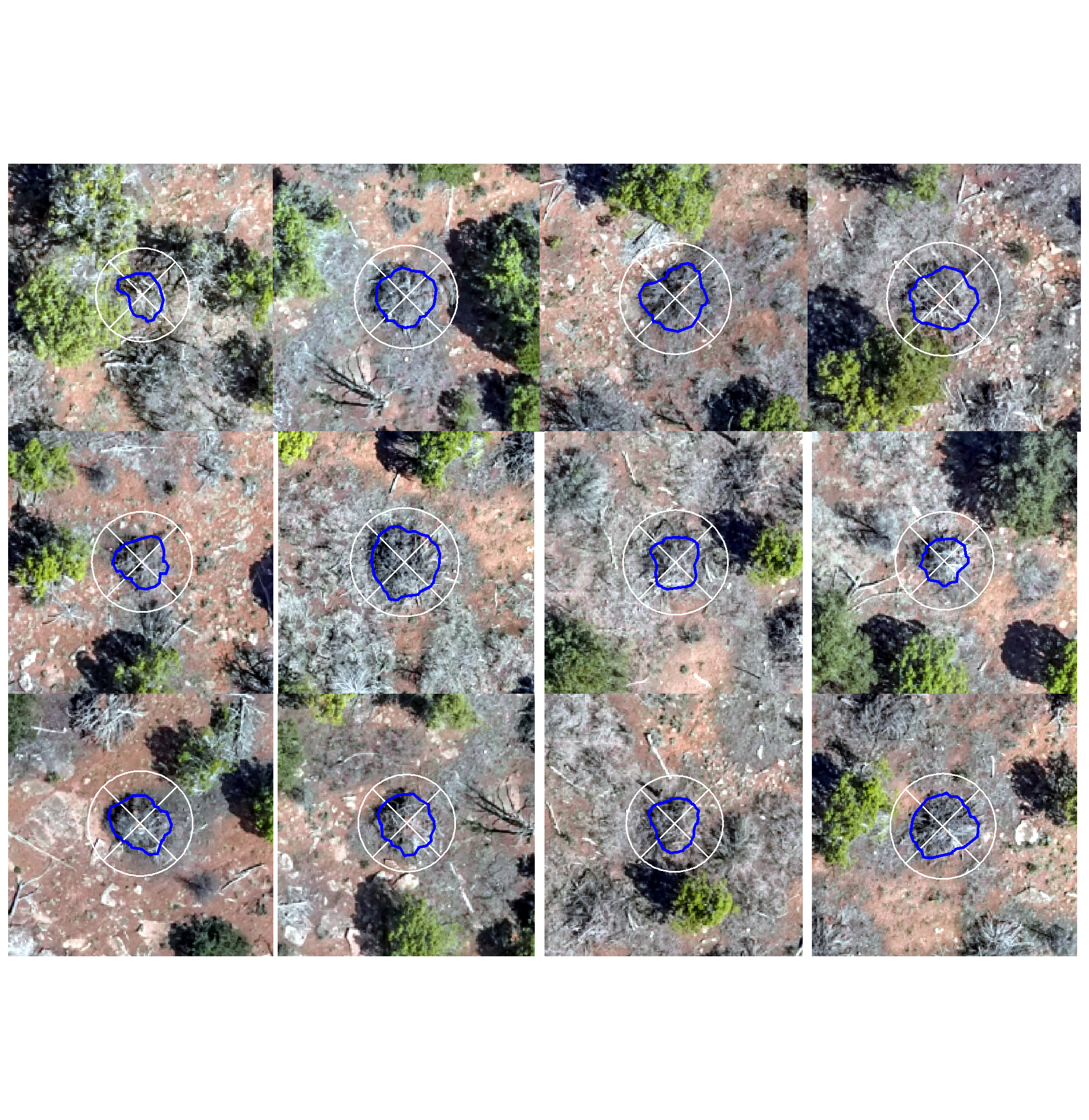
yeah, those don’t line up very well ;/ … however, we’ll continue using the field-measured height and diameter to further explore our form quantification error
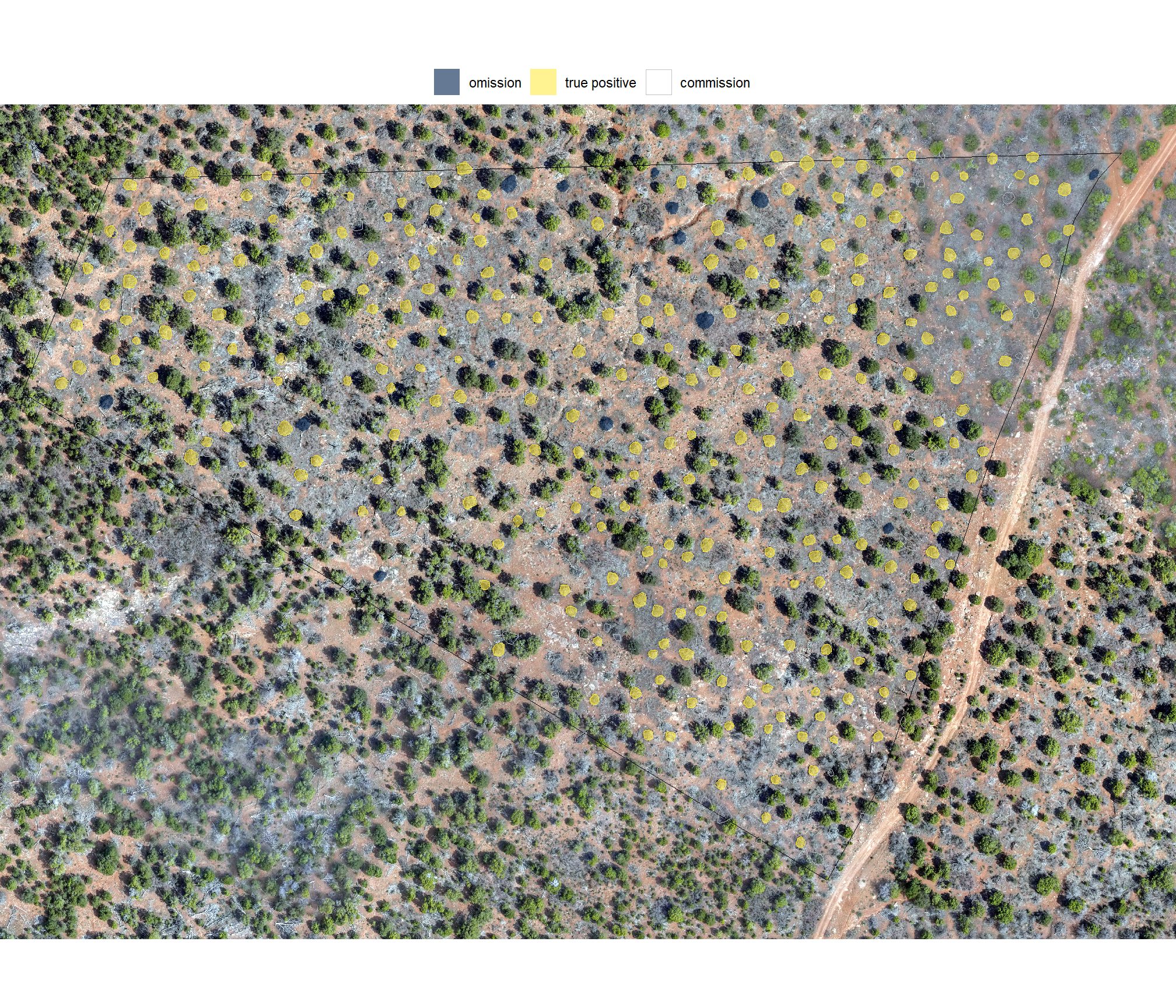
what is the distribution of the ground truth and prediction matching classification?
# what did we get?
ground_truth_prediction_match_ans %>%
  dplyr::count(match_grp) %>%
  dplyr::mutate(pct = (n/sum(n)) %>% scales::percent(accuracy=0.1))
## # A tibble: 3 × 3
## match_grp n pct
## <ord> <int> <chr>
## 1 omission 15 4.2%
## 2 commission 79 22.2%
## 3 true positive 262 73.6%let’s look at that spatially
pal_match_grp <- c(
  "omission"=viridis::cividis(3)[1]
  , "commission"= "gray77" #viridis::cividis(3)[2]
  , "true positive"=viridis::cividis(3)[3]
)
# plot it
ortho_plt_fn(
  my_ortho_rast = pj_rgb_rast
  , stand = pj_stand_boundary %>%
    dplyr::ungroup() %>%
    sf::st_union() %>%
    sf::st_bbox() %>%
    sf::st_as_sfc() %>%
    sf::st_transform(terra::crs(pj_rgb_rast))
  , buffer = 3
) +
# ggplot2::ggplot() +
  ggplot2::geom_sf(
    data =
      pj_stand_boundary %>%
      sf::st_transform(terra::crs(pj_rgb_rast))
    , color = "black", fill = NA
  ) +
  ggplot2::geom_sf(
    data =
      pj_slash_piles_polys %>%
      dplyr::filter(is_in_stand) %>%
      sf::st_transform(sf::st_crs(final_predicted_slash_piles)) %>%
      dplyr::left_join(
        ground_truth_prediction_match_ans %>%
          dplyr::select(pile_id,match_grp)
        , by = "pile_id"
      ) %>%
      sf::st_transform(terra::crs(pj_rgb_rast))
    , mapping = ggplot2::aes(fill = match_grp)
    , color = NA ,alpha=0.6
  ) +
  ggplot2::geom_sf(
    data =
      final_predicted_slash_piles %>%
      dplyr::filter(is_in_stand) %>%
      dplyr::left_join(
        ground_truth_prediction_match_ans %>%
          dplyr::select(pred_id,match_grp)
        , by = "pred_id"
      ) %>%
      sf::st_transform(terra::crs(pj_rgb_rast))
    , mapping = ggplot2::aes(fill = match_grp, color = match_grp)
    , alpha = 0
    , lwd = 0.3
  ) +
  ggplot2::scale_fill_manual(values = pal_match_grp, name = "") +
  ggplot2::scale_color_manual(values = pal_match_grp, name = "") +
  ggplot2::theme_void() +
  ggplot2::theme(legend.position = "top") +
  ggplot2::guides(
    fill = ggplot2::guide_legend(override.aes = list(color = c(NA,NA,pal_match_grp["commission"])))
    , color = "none"
  )
10.4.4.4 Instance level (pile level)
let’s look at the pile-level data directly to evaluate the true positive detections, omissions (false negatives), and commissions (false positives)
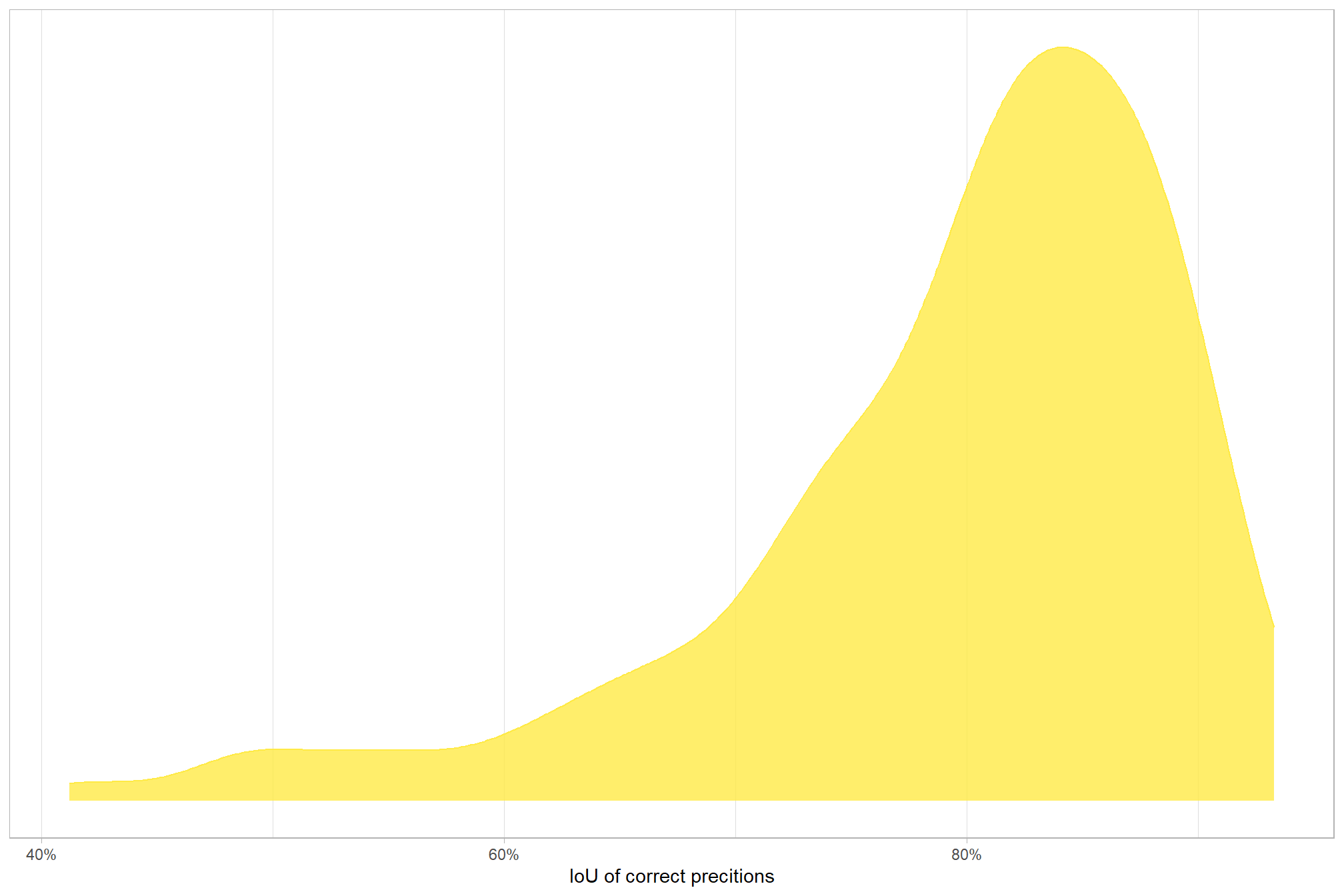
let’s quickly look at the IoU values on the true positives
ground_truth_prediction_match_ans %>%
  dplyr::filter(match_grp=="true positive") %>%
  dplyr::select(iou) %>%
  summary()
## iou
## Min. :0.4124
## 1st Qu.:0.7523
## Median :0.8182
## Mean :0.7944
## 3rd Qu.:0.8639
## Max. :0.9326for the majority (i.e. >95%) of matches, the IoU was above 58.3%
here is the distribution of IoU for those matches
ground_truth_prediction_match_ans %>%
  dplyr::filter(match_grp=="true positive") %>%
  ggplot2::ggplot(mapping = ggplot2::aes(x = iou, color = match_grp, fill = match_grp)) +
  ggplot2::geom_density(mapping = ggplot2::aes(y=ggplot2::after_stat(scaled)), alpha = 0.8) +
  ggplot2::scale_color_manual(values=pal_match_grp) +
  ggplot2::scale_fill_manual(values=pal_match_grp) +
  ggplot2::scale_y_continuous(NULL,breaks=NULL) +
  ggplot2::scale_x_continuous(labels=scales::percent) +
  ggplot2::labs(
    color="",fill="",x="IoU of correct precitions"
  ) +
  ggplot2::theme_light() +
  ggplot2::theme(
    legend.position = "none"
    , strip.text = ggplot2::element_text(size = 9, face = "bold", color = "black")
  )
is there a difference between the field-measured pile sizes of the true positive detections and the omissions (false negative)?
let’s compare the field-measured height and diameter and the image-annotated area for omissions and true positives since those measurements exist for both sets
ground_truth_prediction_match_ans %>%
  dplyr::filter(match_grp!="commission") %>%
  dplyr::select(pile_id,match_grp,gt_height_m,gt_diameter_m,gt_area_m2) %>%
  tidyr::pivot_longer(cols = -c(pile_id,match_grp)) %>%
  dplyr::mutate(
    name = factor(
      name
      , ordered = T
      , levels = c("gt_height_m","gt_diameter_m","gt_area_m2")
      , labels = c(
        "height (m)","diameter (m)"
        , "image annotated area (m2)"
      )
    )
  ) %>%
  ggplot2::ggplot(mapping = ggplot2::aes(x = value, color = match_grp, fill = match_grp)) +
  ggplot2::geom_density(mapping = ggplot2::aes(y=ggplot2::after_stat(scaled)), alpha = 0.7) +
  ggplot2::facet_grid(cols = dplyr::vars(name), scales = "free_x") +
  ggplot2::scale_color_manual(values=pal_match_grp) +
  ggplot2::scale_fill_manual(values=pal_match_grp) +
  ggplot2::scale_y_continuous(NULL,breaks=NULL) +
  ggplot2::labs(
    color="",fill="",x=""
    , subtitle = "ground truth form measurements"
  ) +
  ggplot2::theme_light() +
  ggplot2::theme(
    legend.position = "top"
    , strip.text = ggplot2::element_text(size = 9, face = "bold", color = "black")
  )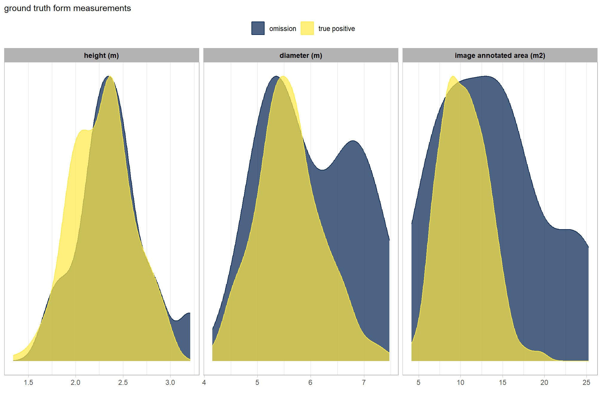
wow! note that we did not inspect the field-collected and image-annotated ground truth measurement data prior to implementing our remote-sensing based pile detection methodology. we purposefully did not look at this data until after making the predictions because we wanted to set up our remote sensing pile detection method without as if we did not measure a single pile in the field so as to not bias our implementation of the method. to implement this remote sensing method slash pile detection framework in practice, we would likely not have any field-measured data on pile structure and if we did it would only be for a very small sample of piles. remember, the entire objective of creating this method is so that time in the field can be minimized to the time needed to visually assess the treatment implementation to acquire quick observational anecdotes and potentially measure some sample piles and then fly a UAS data collection mission to get the data needed to implement this method. compare that minimal time to the traditional, field-based method of slash pile identification and measurement which is much more costly in terms of time and personnel needed.
visually, there is minimal difference in the form measurements between the ground truth piles that were correctly identified as true postive matches and those that were missed by the detection method as omissions (i.e. false negatives). if anything the diameter of the omissions were generally more variable than the diameter of the correct predictions.
we can also see from these distributions of field-collected height and diameter and pile area from the image-annotated ground truth data that, compared to the pile construction prescription, piles were mostly between 1.75-3m in height with an diameters between 4.5-7m compared to the prescription which called for minimum heights and diameters of 1.5m though no maximum was specified. these measurments validate our decision to use a much larger expected pile area multiplier compared to the prescription minimum than we did for the height multiplier when we parameterized the detection methodology using the max_ht_m and max_area_m2 parameters.
let’s now look at the summary stats of ground truth piles
kbl_form_sum_stats(
  pj_slash_piles_polys %>% dplyr::filter(is_in_stand) %>% dplyr::select(!tidyselect::contains("volume_m3"))
  , caption = "Ground Truth Piles: summary statistics for form measurements<br>pinyon-juniper validation site"
)| # piles | Metric | Mean | Std Dev | q 10% | Median | q 90% | Range |
|---|---|---|---|---|---|---|---|
| 277 | Height m | 2.3 | 0.3 | 1.9 | 2.3 | 2.7 | 1.3—3.2 |
| Diameter m (field) | 5.6 | 0.6 | 4.9 | 5.5 | 6.5 | 4.2—7.5 | |
| Diameter m (image) | 4.2 | 0.6 | 3.4 | 4.1 | 4.9 | 2.6—6.4 | |
| Area m2 (image) | 10.6 | 3.2 | 6.8 | 10.4 | 14.4 | 4.1—25.3 |
and let’s look at the summary stats of the predicted piles
kbl_form_sum_stats(
  final_predicted_slash_piles %>% dplyr::filter(is_in_stand)
  , caption = "Predicted Piles: summary statistics for form measurements<br>pinyon-juniper validation site"
)| # piles | Metric | Mean | Std Dev | q 10% | Median | q 90% | Range |
|---|---|---|---|---|---|---|---|
| 341 | Height m | 1.3 | 0.5 | 0.8 | 1.1 | 2.1 | 0.4—2.3 |
| Diameter m | 3.7 | 0.8 | 2.6 | 3.8 | 4.7 | 2.0—7.3 | |
| Area m2 | 8.3 | 3.5 | 3.6 | 8.5 | 12.9 | 2.2—17.0 | |
| Volume m3 | 4.7 | 2.7 | 1.9 | 4.2 | 7.8 | 0.5—18.4 |
let’s look at some examples on our RGB image
true positive matches (correct predictions)
plts_temp <-
  which(ground_truth_prediction_match_ans$match_grp %in% c("true positive")) %>%
  sample( min(16,agg_ground_truth_match_ans$tp_n) ) %>%
  purrr::map(function(x){
    dta <- ground_truth_prediction_match_ans %>% dplyr::slice(x)
    gt <- pj_slash_piles_polys %>% dplyr::filter(pile_id==dta$pile_id)
    pr <- final_predicted_slash_piles %>% dplyr::filter(pred_id==dta$pred_id)
    #plt
    ortho_plt_fn(my_ortho_rast=pj_rgb_rast, stand=sf::st_union(gt,pr), buffer=6) +
      ggplot2::geom_sf(data = gt, fill = NA, color = "blue", lwd = 0.6) +
      ggplot2::geom_sf(data = pr, fill = NA, color = "brown", lwd = 0.5)
  })
# combine
patchwork::wrap_plots(
  plts_temp
  , ncol = 4
)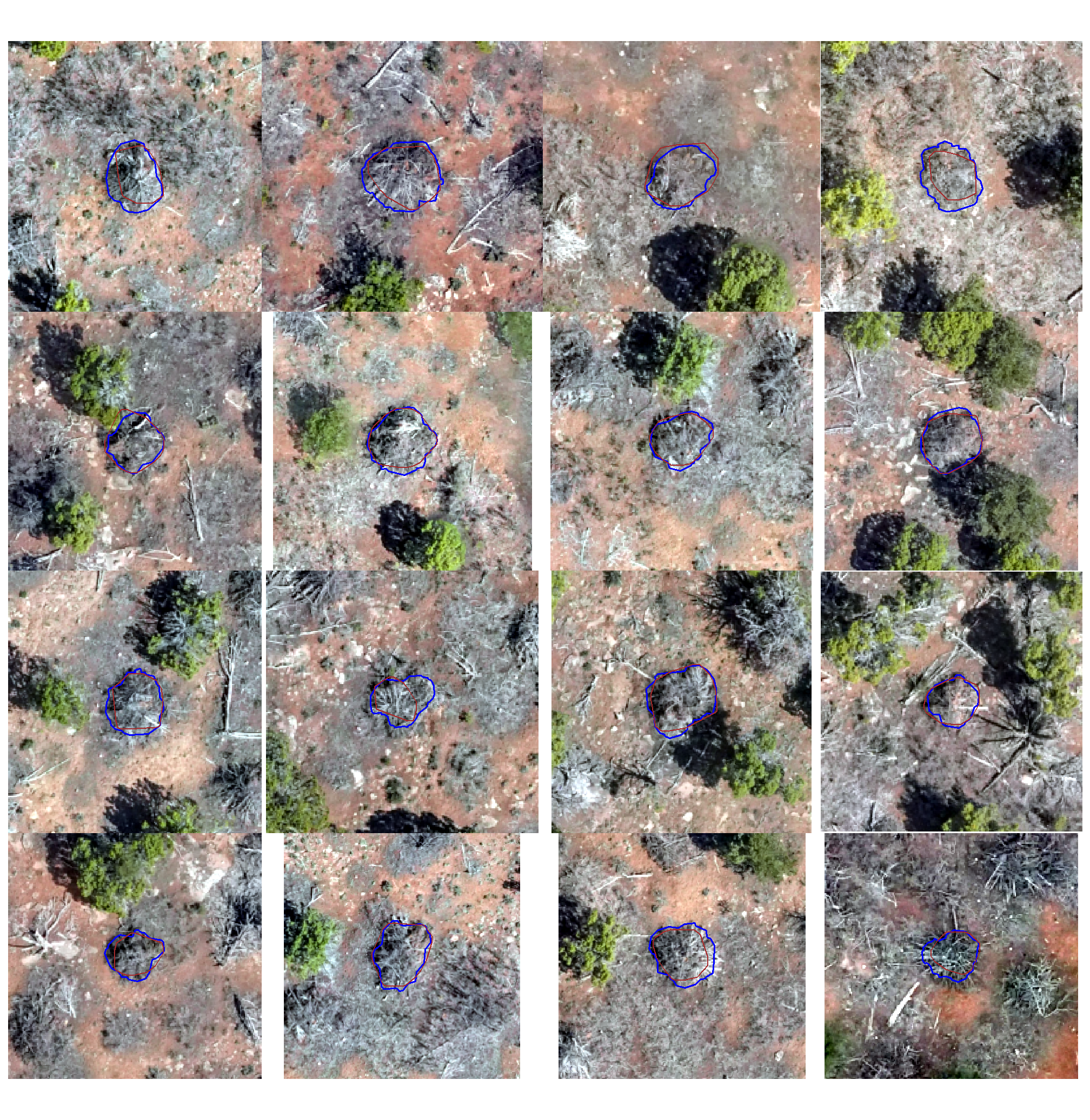
omissions (false negatives)
plts_temp <-
  which(ground_truth_prediction_match_ans$match_grp %in% c("omission")) %>%
  sample( min(16,agg_ground_truth_match_ans$fn_n) ) %>%
  purrr::map(function(x){
    dta <- ground_truth_prediction_match_ans %>% dplyr::slice(x)
    gt <- pj_slash_piles_polys %>% dplyr::filter(pile_id==dta$pile_id)

    #plt
    ortho_plt_fn(my_ortho_rast=pj_rgb_rast, stand=sf::st_union(gt), buffer=6) +
      ggplot2::geom_sf(data = gt, fill = NA, color = "blue", lwd = 0.6)
  })
# combine
patchwork::wrap_plots(
  plts_temp
  , ncol = 4
)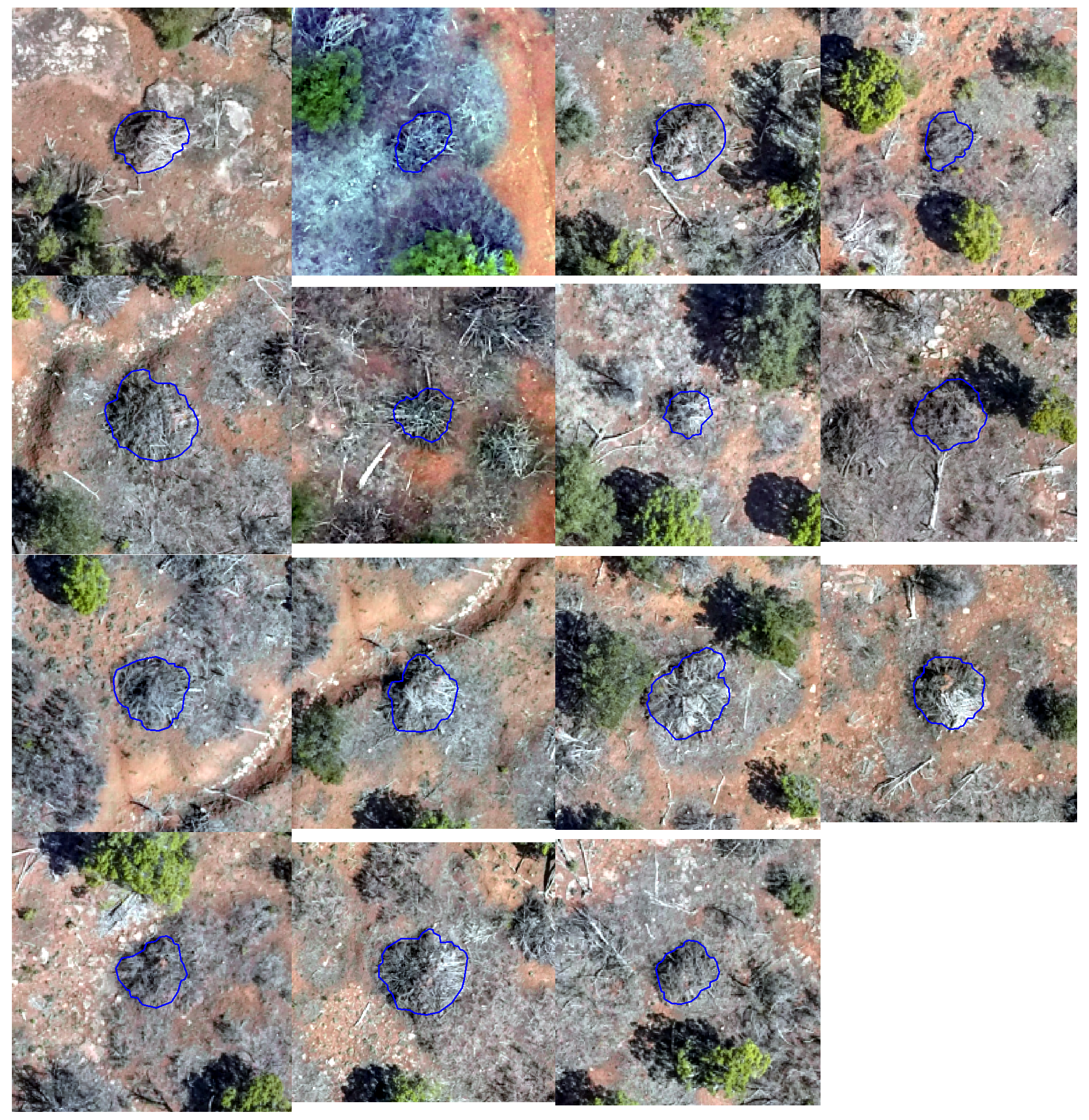
let’s add the CHM to that plot to see if it helps shed light on why these were missed
# plot RGB + CHM
plts_temp <-
  which(ground_truth_prediction_match_ans$match_grp %in% c("omission")) %>%
  sample( min(12,agg_ground_truth_match_ans$fn_n) ) %>%
  purrr::map(function(x){
    dta <- ground_truth_prediction_match_ans %>% dplyr::slice(x)
    gt <- pj_slash_piles_polys %>% dplyr::filter(pile_id==dta$pile_id)
    #plt
    ortho_plt_fn(my_ortho_rast=pj_rgb_rast, stand=sf::st_union(gt), buffer=6) +
      ggnewscale::new_scale_fill() +
      ggplot2::geom_tile(
        data = chm_rast_stand %>%
          terra::crop(
            sf::st_union(gt) %>%
              sf::st_transform(terra::crs(chm_rast_stand)) %>%
              terra::vect()
          ) %>%
          terra::mask(
            sf::st_union(gt) %>%
              sf::st_transform(terra::crs(chm_rast_stand)) %>%
              terra::vect()
          ) %>%
          # slice the chm below our desired height
          # this is what slash_pile_detect_watershed() does
          # terra::clamp(upper = 2.3, lower = 0, values = F) %>%
          terra::as.data.frame(xy=T) %>%
          dplyr::rename(f=3)
        , mapping = ggplot2::aes(x=x,y=y,fill=f)
        , alpha = 0.5
      ) +
      ggplot2::scale_fill_viridis_c(option = "plasma", na.value = "gray",name = "CHM (m)") +
      ggplot2::geom_sf(data = gt, fill = NA, color = "blue", lwd = 0.6) +
      ggplot2::labs(
        subtitle = paste0(
          "pile ID: ", dta$pile_id
          , "\nGT area: ", round(dta$gt_area_m2,1)
          # , " | Pred ht: ", round(dta$pred_height_m,1)
          , "\nGT dia: ", round(dta$gt_diameter_m,1)
          # , " | Pred dia: ", round(dta$pred_diameter_m,1)
        )
      ) +
      ggplot2::theme(legend.text = ggplot2::element_text(size = 6),legend.title = ggplot2::element_text(size = 6))
  })
# plts_temp
# combine
patchwork::wrap_plots(
  plts_temp
  , ncol = 4
)
now, let’s check out the predicted sizes of the commissions (false positives) compared to the predicted sizes of the predicted piles that were correctly matched with the ground truth data
let’s compare the predicted height, diameter, area for commissions and true positives since those measurements exist for both sets
ground_truth_prediction_match_ans %>%
  dplyr::filter(match_grp!="omission") %>%
  dplyr::select(pile_id,match_grp,pred_height_m,pred_diameter_m,pred_area_m2) %>%
  tidyr::pivot_longer(cols = -c(pile_id,match_grp)) %>%
  dplyr::mutate(
    name = factor(
      name
      , ordered = T
      , levels = c("pred_height_m","pred_diameter_m","pred_area_m2")
      , labels = c(
        "predicted height (m)","predicted diameter (m)"
        , "predicted area (m2)"
      )
    )
  ) %>%
  ggplot2::ggplot(mapping = ggplot2::aes(x = value, color = match_grp, fill = match_grp)) +
  ggplot2::geom_density(mapping = ggplot2::aes(y=ggplot2::after_stat(scaled)), alpha = 0.7) +
  ggplot2::facet_grid(cols = dplyr::vars(name), scales = "free_x") +
  ggplot2::scale_color_manual(values=pal_match_grp) +
  ggplot2::scale_fill_manual(values=pal_match_grp) +
  ggplot2::scale_y_continuous(NULL,breaks=NULL) +
  ggplot2::labs(color="",fill="",x="") +
  ggplot2::theme_light() +
  ggplot2::theme(
    legend.position = "top"
    , strip.text = ggplot2::element_text(size = 9, face = "bold", color = "black")
  )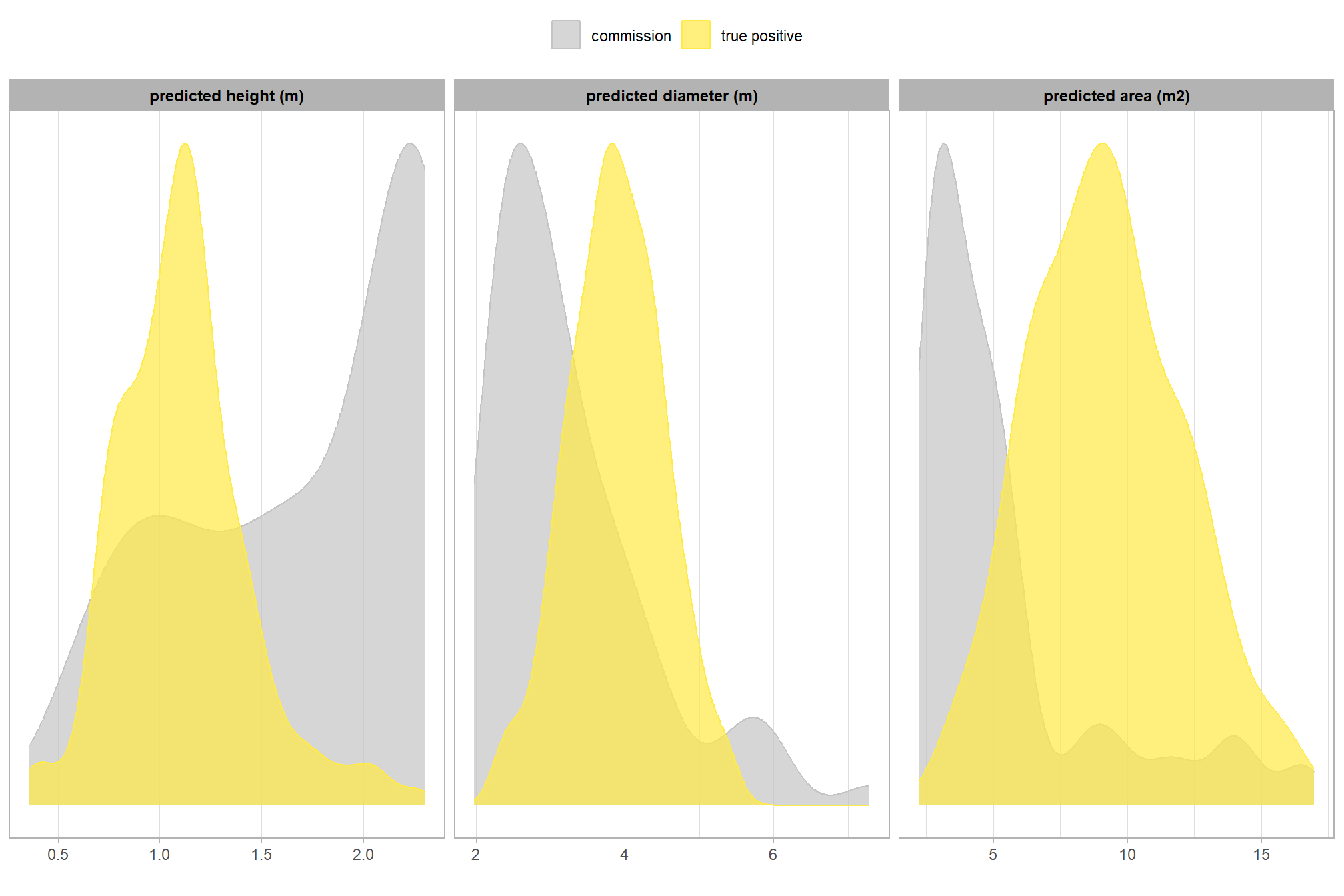
this is interesting, the incorrectly predicted piles generally had a much smaller footprint (i.e diameter and area) than the predicted piles that correctly match to actual piles. in terms of height, there were two distinct groups of incorrect predictions, some that were in-line with the correctly predicted piles and some that were much taller than the correct predictions.
let’s table the predicted form measurements
ground_truth_prediction_match_ans %>%
  dplyr::filter(match_grp!="omission") %>%
  dplyr::select(pile_id,match_grp,pred_height_m,pred_diameter_m,pred_area_m2) %>%
  dplyr::group_by(match_grp) %>%
  dplyr::summarise(
    dplyr::across(
      c(pred_height_m,pred_diameter_m,pred_area_m2)
      , .fns = list(
        mean = ~mean(.x,na.rm=T)
        , sd = ~sd(.x,na.rm=T)
        , q10 = ~quantile(.x,na.rm=T,probs=0.1)
        , q50 = ~quantile(.x,na.rm=T,probs=0.5)
        , q90 = ~quantile(.x,na.rm=T,probs=0.9)
        , min = ~min(.x,na.rm=T)
        , max = ~max(.x,na.rm=T)
      )
    )
    , n = dplyr::n()
  ) %>%
  dplyr::ungroup() %>%
  tidyr::pivot_longer(cols = -c( match_grp,n)) %>%
  dplyr::mutate(
    agg = stringr::word(name,-1,sep = "_")
    , metric = stringr::str_remove_all(name, paste0("_",agg))
  ) %>%
  dplyr::select(-name) %>%
  dplyr::mutate(
    value = dplyr::case_when(
      metric == "gt_height_m" ~ scales::comma(value,accuracy=0.1)
      , T ~ scales::comma(value,accuracy=0.1)
    )
  ) %>%
  tidyr::pivot_wider(names_from = agg, values_from = value) %>%
  dplyr::mutate(
    range = paste0(min, "—", max)
  ) %>%
  dplyr::arrange( match_grp, desc(n)) %>%
  dplyr::select(-c(n,min,max)) %>%
  dplyr::relocate(match_grp) %>%
  dplyr::mutate(
    metric = factor(
      metric
      , ordered = T
      , levels = c("pred_height_m","pred_diameter_m","pred_area_m2")
      , labels = c(
        "predicted height (m)","predicted diameter (m)"
        , "predicted area (m2)"
      )
    )
  ) %>%
  kableExtra::kbl(
    caption = "Predicted Piles: summary statistics for form measurements"
    , col.names = c(
      "segmentation<br>classification", "Metric"
      , "Mean"
      , "Std Dev"
      , "q 10%", "Median", "q 90%"
      , "Range"
    )
    , escape = F
    # , digits = 2
  ) %>%
  kableExtra::kable_styling(font_size = 13) %>%
kableExtra::collapse_rows(columns = 1, valign = "top")|
segmentation classification |
Metric | Mean | Std Dev | q 10% | Median | q 90% | Range |
|---|---|---|---|---|---|---|---|
| commission | predicted height (m) | 1.7 | 0.6 | 0.8 | 1.9 | 2.3 | 0.5—2.3 |
| predicted diameter (m) | 3.2 | 1.1 | 2.3 | 3.0 | 4.6 | 2.0—7.3 | |
| predicted area (m2) | 5.4 | 3.6 | 2.5 | 4.1 | 11.2 | 2.2—16.6 | |
| true positive | predicted height (m) | 1.1 | 0.3 | 0.8 | 1.1 | 1.5 | 0.4—2.3 |
| predicted diameter (m) | 3.9 | 0.6 | 3.1 | 3.9 | 4.7 | 2.3—5.4 | |
| predicted area (m2) | 9.2 | 2.9 | 5.8 | 9.1 | 13.1 | 2.9—17.0 |
let’s look at some examples on our RGB image
commissions (false positives)
plts_temp <-
  which(ground_truth_prediction_match_ans$match_grp %in% c("commission")) %>%
  sample( min(16,agg_ground_truth_match_ans$fp_n) ) %>%
  purrr::map(function(x){
    dta <- ground_truth_prediction_match_ans %>% dplyr::slice(x)
    pr <- final_predicted_slash_piles %>% dplyr::filter(pred_id==dta$pred_id)
    #plt
    ortho_plt_fn(my_ortho_rast=pj_rgb_rast, stand=sf::st_union(pr), buffer=6) +
      ggplot2::geom_sf(data = pr, fill = NA, color = "brown", lwd = 0.5)
  })
# combine
patchwork::wrap_plots(
  plts_temp
  , ncol = 4
)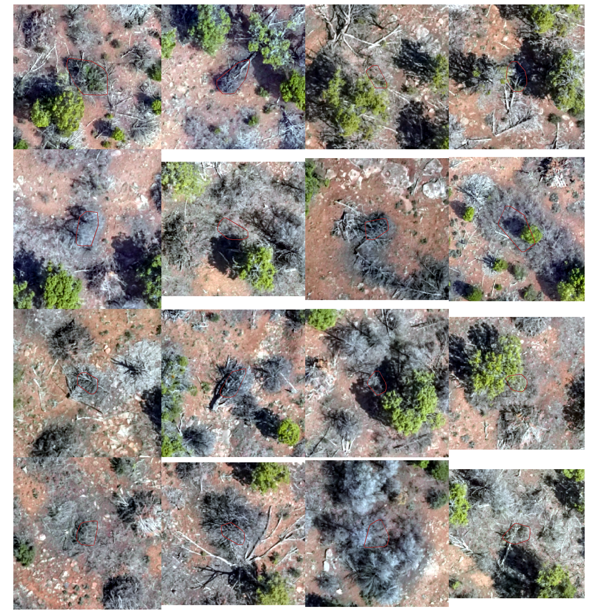
it is difficult to tell from the RGB imagery alone what those actually are and why they might have been improperly predicted as slash piles. let’s look at the point cloud for some to see if we can determine what the issue is
first the RGB
# it's difficult to see why those false positives were included and not filtered out by the spectral filtering
# plot some point clouds
# cloud2trees::cloud2raster() output of normalized las
norm_las_ctg <- lidR::readLAScatalog( file.path(c2t_output_dir, "point_cloud_processing_temp","02_normalize") )
lidR::opt_progress(norm_las_ctg) <- F
# sample piles
ex_piles_temp <- which(ground_truth_prediction_match_ans$match_grp %in% c("commission")) %>% sample(2)
# rgb plot
pr_temp <- final_predicted_slash_piles %>%
  dplyr::inner_join(
    ground_truth_prediction_match_ans %>%
      dplyr::slice(ex_piles_temp[1]) %>%
      dplyr::select(pred_id)
  )
#plt
ortho_plt_fn(my_ortho_rast=pj_rgb_rast, stand=sf::st_union(pr_temp), buffer=3) +
  ggplot2::geom_sf(data = pr_temp, fill = NA, color = "brown", lwd = 0.8)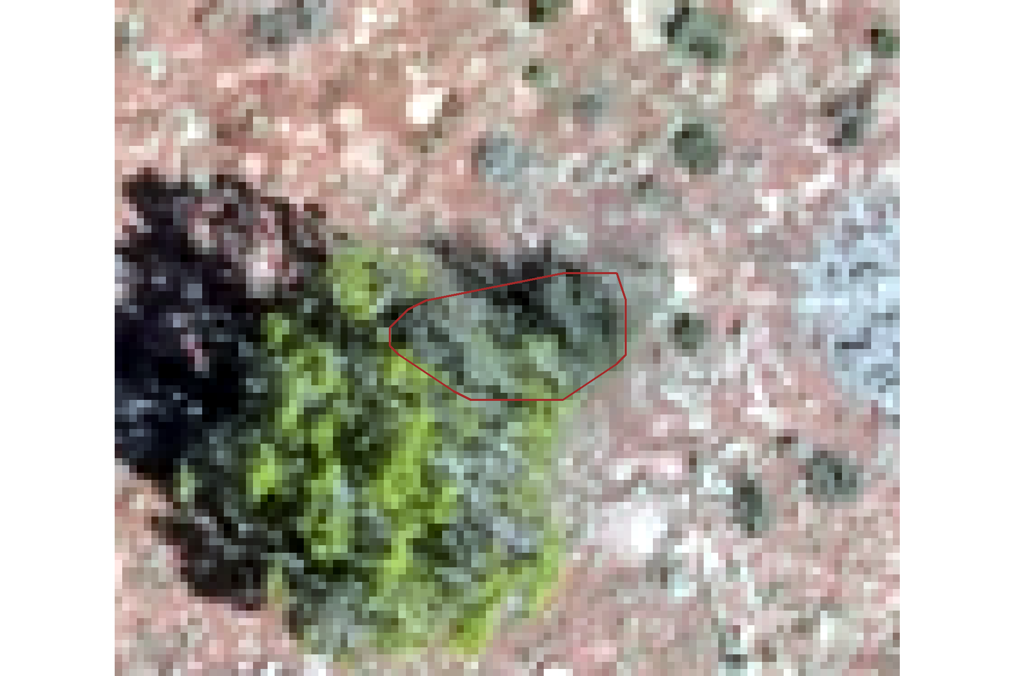
what even is that?
i mean, it could be a pile
let’s try another sample. first the RGB
# rgb plot
pr_temp <- final_predicted_slash_piles %>%
  dplyr::inner_join(
    ground_truth_prediction_match_ans %>%
      dplyr::slice(ex_piles_temp[2]) %>%
      dplyr::select(pred_id)
  )
#plt
ortho_plt_fn(my_ortho_rast=pj_rgb_rast, stand=sf::st_union(pr_temp), buffer=3) +
  ggplot2::geom_sf(data = pr_temp, fill = NA, color = "brown", lwd = 0.8)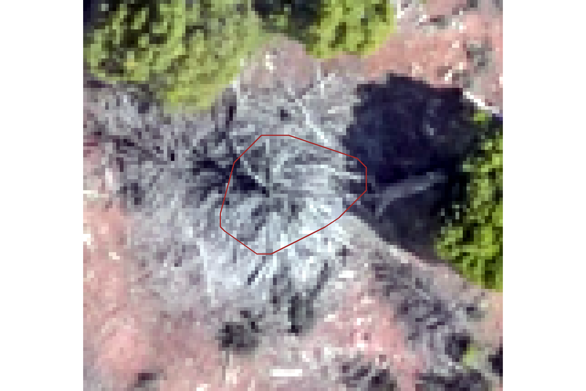
huh?
id even k.
10.4.5 Volume Comparison
Previously, we explored differences in the allometric field volume and predicted volume for the optimal training results. See that section introduction for the full details on what we are doing and why…
welcome back…Let’s make the same comparisons for these validation data. We fully expect there to be much larger differences in volume based on the suspicious field-measured height and diameter values.
we already added volume measurements to the TP matches for both the ground truth and predicted piles, summary of that data
ground_truth_prediction_match_ans %>%
  dplyr::filter(match_grp=="true positive",!is.na(gt_volume_m3), !is.na(pred_volume_m3)) %>%
  dplyr::select(gt_volume_m3, pred_volume_m3) %>%
  summary()
## gt_volume_m3 pred_volume_m3
## Min. : 9.371 Min. : 0.5414
## 1st Qu.:22.558 1st Qu.: 3.0780
## Median :27.826 Median : 4.4526
## Mean :28.667 Mean : 4.7432
## 3rd Qu.:33.683 3rd Qu.: 6.2125
## Max. :57.247 Max. :11.4447those don’t really look like they match up well…let’s explore
ground_truth_prediction_match_ans %>%
  dplyr::filter(match_grp=="true positive",!is.na(gt_volume_m3), !is.na(pred_volume_m3)) %>%
  dplyr::mutate(diff_volume_m3 = gt_volume_m3 - pred_volume_m3) %>%
  ggplot2::ggplot(mapping = ggplot2::aes(y = gt_volume_m3, x = pred_volume_m3)) +
  ggplot2::geom_abline(lwd = 1.5) +
  # ggplot2::geom_point(ggplot2::aes(color = diff_volume_m3)) +
  ggplot2::geom_point(color = "navy") +
  ggplot2::geom_smooth(method = "lm", se=F, color = "tomato", linetype = "dashed") +
  ggplot2::scale_color_viridis_c(option = "mako", direction = -1, alpha = 0.8) +
  ggplot2::scale_x_continuous(limits = c(0, max( max(ground_truth_prediction_match_ans$pred_volume_m3,na.rm=T), max(ground_truth_prediction_match_ans$gt_volume_m3,na.rm=T) ) )) +
  ggplot2::scale_y_continuous(limits = c(0, max( max(ground_truth_prediction_match_ans$pred_volume_m3,na.rm=T), max(ground_truth_prediction_match_ans$gt_volume_m3,na.rm=T) ) )) +
  ggplot2::labs(
    y = latex2exp::TeX("allometric field volume $m^3$")
    , x = latex2exp::TeX("predicted volume $m^3$")
    # , color = "image-field\ndiameter diff."
    , subtitle = latex2exp::TeX("bulk volume ($m^3$) comparison")
  ) +
  ggplot2::theme_light()
this is exactly what we expected: for true positive matches, there is a clear systematic difference with the plot showing that the volume calculated using the idealized, regular shape assumption (allometric field volume) is consistently larger than the predicted volume derived from the CHM
let’s check these using lm()
lm_temp <- lm(
  gt_volume_m3 ~ pred_volume_m3
  , data =
    ground_truth_prediction_match_ans %>%
    dplyr::filter(
        match_grp=="true positive"
        , !is.na(gt_volume_m3), !is.na(pred_volume_m3
      )
    )
)
summary(lm_temp)
##
## Call:
## lm(formula = gt_volume_m3 ~ pred_volume_m3, data = ground_truth_prediction_match_ans %>%
## dplyr::filter(match_grp == "true positive", !is.na(gt_volume_m3),
## !is.na(pred_volume_m3)))
##
## Residuals:
## Min 1Q Median 3Q Max
## -12.855 -4.688 -1.116 4.148 27.828
##
## Coefficients:
## Estimate Std. Error t value Pr(>|t|)
## (Intercept) 16.9148 0.9684 17.47 <2e-16 ***
## pred_volume_m3 2.4777 0.1847 13.41 <2e-16 ***
## ---
## Signif. codes: 0 '***' 0.001 '**' 0.01 '*' 0.05 '.' 0.1 ' ' 1
##
## Residual standard error: 6.638 on 257 degrees of freedom
## Multiple R-squared: 0.4118, Adjusted R-squared: 0.4095
## F-statistic: 179.9 on 1 and 257 DF, p-value: < 2.2e-16These linear model results (intercept = 16.91, slope = 2.48) indicate a strong proportional bias that significantly increases with pile size. This data suggests that the geometric assumptions of the allometric model potentially introduce substantial scaling error which may limit its reliability (especially for larger piles) for accurately estimating the volume of real-world piles which have heterogeneous footprints and elevation profiles.
before we compare the volume measurements in aggregate, let’s look at their distributions
vol_df_temp <-
  ground_truth_prediction_match_ans %>%
  dplyr::filter(match_grp=="true positive",!is.na(gt_volume_m3), !is.na(pred_volume_m3)) %>%
  dplyr::select(pile_id,gt_volume_m3,pred_volume_m3) %>%
  tidyr::pivot_longer(cols = -c(pile_id)) %>%
  dplyr::mutate(
    name = factor(
      name
      , ordered = T
      , levels = c("gt_volume_m3","pred_volume_m3")
      , labels = c(
        "allometric field volume"
        , "predicted volume"
      )
    )
  )
# plot dist
vol_df_temp %>%
  ggplot2::ggplot(mapping = ggplot2::aes(x = value, color = name, fill = name)) +
  ggplot2::geom_density(mapping = ggplot2::aes(y=ggplot2::after_stat(scaled)), alpha = 0.7) +
  harrypotter::scale_color_hp_d(option = "lunalovegood") +
  harrypotter::scale_fill_hp_d(option = "lunalovegood") +
  ggplot2::scale_y_continuous(NULL,breaks=NULL) +
  ggplot2::labs(
    color="",fill="",x=latex2exp::TeX("volume $m^3$")
    , subtitle = latex2exp::TeX("bulk volume ($m^3$) comparison of distributions")
  ) +
  ggplot2::theme_light() +
  ggplot2::theme(
    legend.position = "top"
  )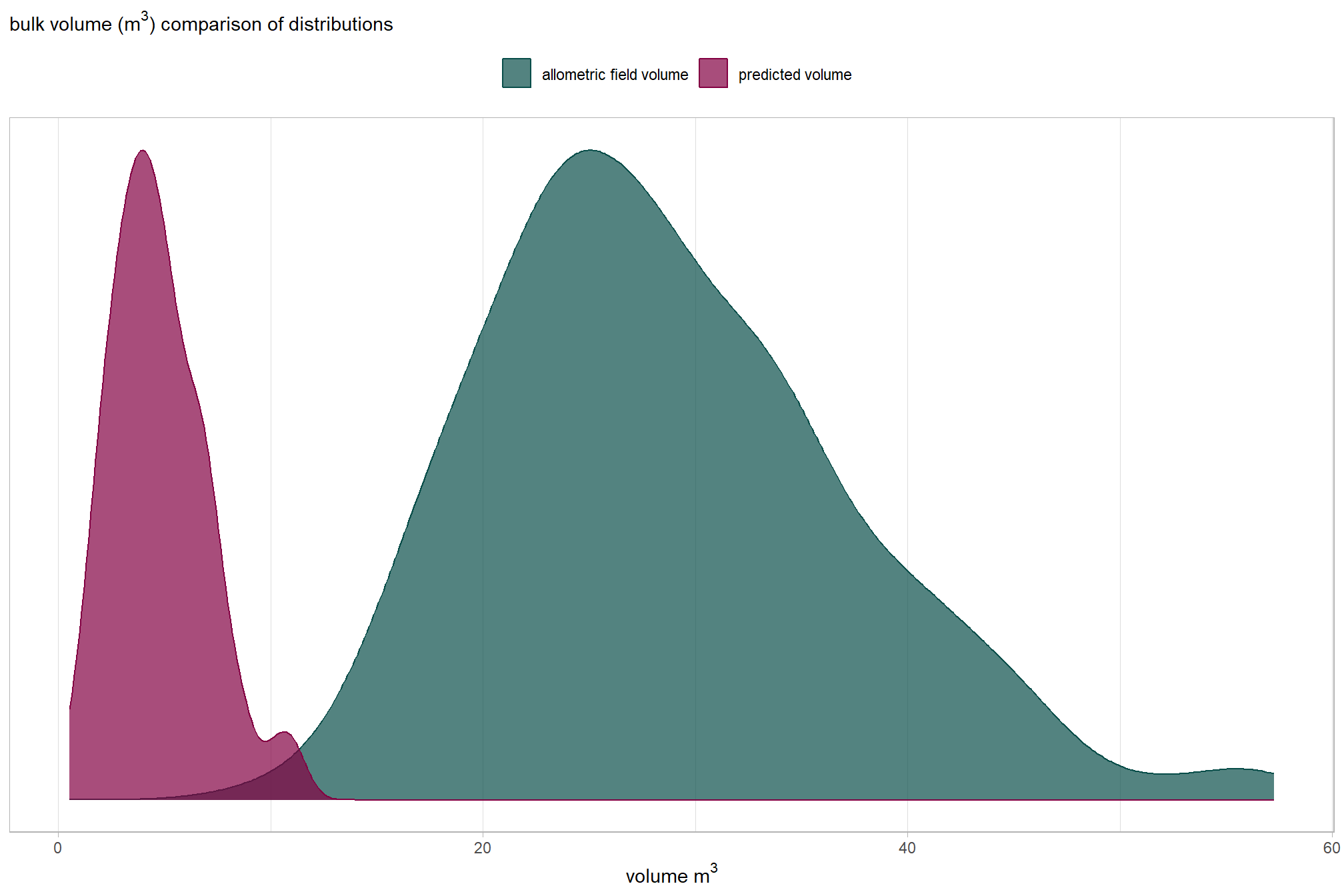
slope plots are neat too
vol_df_temp %>%
  ggplot2::ggplot(
    mapping = ggplot2::aes(x = name, y = value, group = pile_id)
  ) +
  ggplot2::geom_line(key_glyph = "point", alpha = 0.7, color = "gray", lwd = 1.1) +
  ggplot2::geom_point(mapping = ggplot2::aes(color = name), alpha = 0.7, size = 2.5) +
  harrypotter::scale_color_hp_d(option = "lunalovegood") +
  ggplot2::labs(
    color=""
    , y = latex2exp::TeX("volume $m^3$")
    , x = ""
    , subtitle = latex2exp::TeX("bulk volume ($m^3$) comparison at the pile level")
  ) +
  ggplot2::theme_light() +
  ggplot2::theme(
    legend.position = "none"
    , axis.title = ggplot2::element_text(size = 10)
    , axis.text = ggplot2::element_text(size = 10)
  )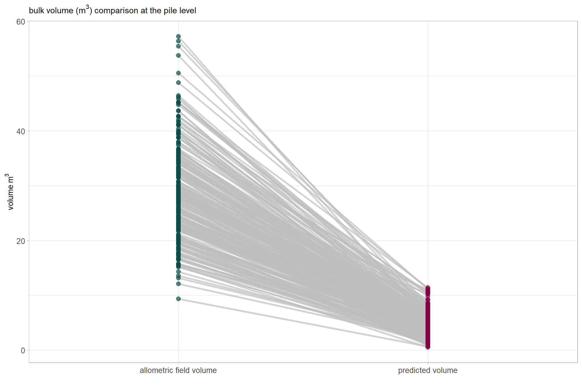
what if we only look at the smaller piles?
vol_df_temp %>%
  dplyr::filter(
    value < quantile(vol_df_temp$value, probs = 0.966)
  ) %>%
  ggplot2::ggplot(
    mapping = ggplot2::aes(x = name, y = value, group = pile_id)
  ) +
  ggplot2::geom_line(key_glyph = "point", alpha = 0.7, color = "gray", lwd = 1.1) +
  ggplot2::geom_point(mapping = ggplot2::aes(color = name), alpha = 0.7, size = 2.5) +
  harrypotter::scale_color_hp_d(option = "lunalovegood") +
  ggplot2::labs(
    color=""
    , y = latex2exp::TeX("volume $m^3$")
    , x = ""
    , subtitle = latex2exp::TeX("bulk volume ($m^3$) comparison at the pile level for the smaller piles")
  ) +
  ggplot2::theme_light() +
  ggplot2::theme(
    legend.position = "none"
    , axis.title = ggplot2::element_text(size = 10)
    , axis.text = ggplot2::element_text(size = 10)
  )
let’s compare aggregated volume measurements for the true positive matches
Mean Difference (MD): \[\text{MD} = \frac{1}{N} \sum_{i=1}^{N} (\text{Allometric Volume}_i - \text{Predicted Volume}_i)\]
Percent Mean Difference: \[\%\text{MD} = \frac{\text{MD}}{\text{Mean}(\text{Predicted Volume})} \times 100\]
vol_agg_df_temp <-
  ground_truth_prediction_match_ans %>%
  dplyr::filter(match_grp=="true positive",!is.na(gt_volume_m3), !is.na(pred_volume_m3)) %>%
  dplyr::ungroup() %>%
  dplyr::summarise(
    mean_diff = mean(gt_volume_m3-pred_volume_m3)
    , sd_diff = sd(gt_volume_m3-pred_volume_m3)
    , mean_gt_volume_m3 = mean(gt_volume_m3,na.rm = T)
    , mean_pred_volume_m3 = mean(pred_volume_m3,na.rm = T)
  ) %>%
  dplyr::mutate(
    pct_mean_diff = mean_diff/mean_pred_volume_m3
  )
what did we get?
vol_agg_df_temp %>%
  tidyr::pivot_longer(dplyr::everything()) %>%
  dplyr::mutate(
    value =
      dplyr::case_when(
        stringr::str_starts(name, "pct_") ~ scales::percent(value, accuracy = 0.1)
        , T ~ scales::comma(value, accuracy = 0.1)
      )
  ) %>%
  kableExtra::kbl(
    caption = "comparison of aggregated allometric field volume and predicted volume"
    , col.names = c("metric", "value")
  ) %>%
kableExtra::kable_styling()| metric | value |
|---|---|
| mean_diff | 23.9 |
| sd_diff | 7.4 |
| mean_gt_volume_m3 | 28.7 |
| mean_pred_volume_m3 | 4.7 |
| pct_mean_diff | 504.4% |
we’ll dig into the MD shortly but before we move on let’s focus on the percent mean difference. We calcualted a %MD of 504.4% which indicates a major systematic difference where the allometric field volume is, on average, 504.4% larger than our CHM-predicted volume. This large relative difference shows how much the geometric assumptions inflate the volume compared to the irregular volumes measured by our remote sensing-based method and also point to suspect field measurements of height and diameter
let’s make a Bland-Altman plot to compare the two measurement methods. this plot uses the average of the two measurements (approximate size) on the x-axis and the difference (bias) between the two measurements on the y-axis
ground_truth_prediction_match_ans %>%
  dplyr::filter(match_grp=="true positive",!is.na(gt_volume_m3), !is.na(pred_volume_m3)) %>%
  dplyr::ungroup() %>%
  # calc needed metrics
  dplyr::mutate(
    mean_vol = (gt_volume_m3+pred_volume_m3)/2
    , diff_vol = (gt_volume_m3-pred_volume_m3) # match the order used in vol_agg_df_temp
    , scale_diff = ifelse(diff_vol < 0, -abs(diff_vol) / abs(min(diff_vol)), diff_vol / max(diff_vol))
  ) %>%
  # ggplot() + geom_point(aes(x=diff_vol,y=0, color=scale_diff)) + scale_color_gradient2(mid = "gray", midpoint = 0, low = "red", high = "blue")
  # plot
  ggplot2::ggplot(
    mapping = ggplot2::aes(x = mean_vol, y = diff_vol)
  ) +
  ggplot2::geom_hline(yintercept = 0, color = "black", lwd = 1.2) +
  # mean difference (bias)
  ggplot2::geom_hline(
    yintercept = vol_agg_df_temp$mean_diff
    , linetype = "dashed", color = "blue", lwd = 1
  ) +
  # upper limit
  ggplot2::geom_hline(
    yintercept = vol_agg_df_temp$mean_diff+1.96*vol_agg_df_temp$sd_diff
    , linetype = "dotted", color = "red", lwd = 1
  ) +
  # lower limit
  ggplot2::geom_hline(
    yintercept = vol_agg_df_temp$mean_diff-1.96*vol_agg_df_temp$sd_diff
    , linetype = "dotted", color = "red", lwd = 1
  ) +
  # annotations
  ggplot2::annotate(
    "text"
    , x = Inf
    , y = vol_agg_df_temp$mean_diff
    , label = latex2exp::TeX(
      paste0(
        "mean difference (bias): "
        , scales::comma(vol_agg_df_temp$mean_diff, accuracy = 0.01)
        , " $m^3$"
      )
      , output = "character"
    )
    , vjust = -0.5
    , hjust = 1
    , color = "blue"
    , size = 4
    , parse = TRUE
  ) +
  ggplot2::annotate(
    "text"
    , x = Inf
    , y = vol_agg_df_temp$mean_diff+1.96*vol_agg_df_temp$sd_diff
    , label = latex2exp::TeX(
      paste0(
        "+1.96 SD: "
        , scales::comma(vol_agg_df_temp$mean_diff+1.96*vol_agg_df_temp$sd_diff, accuracy = 0.01)
        , " $m^3$"
      )
      , output = "character"
    )
    , vjust = -0.5
    , hjust = 1
    , color = "red"
    , size = 4
    , parse = TRUE
  ) +
  ggplot2::annotate(
    "text"
    , x = Inf
    , y = vol_agg_df_temp$mean_diff-1.96*vol_agg_df_temp$sd_diff
    , label = latex2exp::TeX(
      paste0(
        "-1.96 SD: "
        , scales::comma(vol_agg_df_temp$mean_diff-1.96*vol_agg_df_temp$sd_diff, accuracy = 0.01)
        , " $m^3$"
      )
      , output = "character"
    )
    , vjust = 1.5
    , hjust = 1
    , color = "red"
    , size = 4
    , parse = TRUE
  ) +
  # points
  ggplot2::geom_point(mapping = ggplot2::aes(color = scale_diff), size = 1.9, alpha = 0.8) +
  ggplot2::scale_color_steps2(mid = "gray", midpoint = 0) +
  ggplot2::labs(
    subtitle = "Bland-Altman plot: allometric field volume vs predicted volume"
    , x = latex2exp::TeX("mean volume ($m^3$)")
    , y = latex2exp::TeX("difference (allometric - predicted volume $m^3$)")
  ) +
  ggplot2::theme_light() +
  ggplot2::theme(legend.position = "none")
yikes. The upward sloping trend on the Bland-Altman plot confirms a severe proportional bias where the difference between the two volume measurements increases dramatically as the piles grow larger. The high mean difference (MD) of 23.92 m3 quantifies this systematic difference. The increasing slope on this plot indicates that the difference is not a constant offset. Instead, the idealized geometric assumptions of the allometric model greatly exaggerate the volume by an increasingly large amount for bigger piles, demonstrating a fundamental size-dependency in the disagreement between the two modeled methods.
Points falling outside the 95% interval on the plot are instances of significant disagreement between the two volumes measurements for those specific data points. These outliers indicate that, for a particular pile, the difference between the allometric field volume and the predicted volume is unusually large, suggesting a potential failure in either the CHM segmentation process, the quality of the original field measurements, the geometric shape assumption, or a combination thereof. We should investigate these extreme disagreements further to see what is happening
before we do that, let’s use a paired t-test to determine if the mean difference (MD) between the allometric field volume and the predicted volume is statistically significant (i.e. significantly different from zero)
# is the mean difference between the two volumes significantly different from zero
ttest_temp <- t.test(
  ground_truth_prediction_match_ans %>%
    dplyr::filter(match_grp == "true positive") %>%
    dplyr::pull(gt_volume_m3)
  , ground_truth_prediction_match_ans %>%
    dplyr::filter(match_grp == "true positive") %>%
    dplyr::pull(pred_volume_m3)
  , paired = TRUE
)
ttest_temp
##
## Paired t-test
##
## data: ground_truth_prediction_match_ans %>% dplyr::filter(match_grp == "true positive") %>% dplyr::pull(gt_volume_m3) and ground_truth_prediction_match_ans %>% dplyr::filter(match_grp == "true positive") %>% dplyr::pull(pred_volume_m3)
## t = 51.996, df = 258, p-value < 2.2e-16
## alternative hypothesis: true mean difference is not equal to 0
## 95 percent confidence interval:
## 23.01761 24.82968
## sample estimates:
## mean difference
## 23.92365the test gave us a mean difference (MD) of 23.92 m3. also, the p-value of 0.00000 is less than 0.05, meaning we should reject the null hypothesis that the true mean difference is zero. this confirms that the systematic difference (or bias) we observed where allometric volume is larger than our predicted volume is statistically significant and not due to random chance.
10.4.5.1 Extreme Volume Disagreements
let’s investigate the extreme disagreements further to see what is happening
bad_vol_df_temp <-
  ground_truth_prediction_match_ans %>%
  dplyr::filter(match_grp=="true positive",!is.na(gt_volume_m3), !is.na(pred_volume_m3)) %>%
  dplyr::ungroup() %>%
  # calc needed metrics
  dplyr::mutate(
    diff_vol = (gt_volume_m3-pred_volume_m3) # match the order used in vol_agg_df_temp
  ) %>%
  dplyr::filter(
    diff_vol > (vol_agg_df_temp$mean_diff+1.96*vol_agg_df_temp$sd_diff)
  )
# what are the differences?
bad_vol_df_temp %>%
  dplyr::select(
    pile_id
    , gt_height_m, pred_height_m, diff_height_m
    , gt_diameter_m, pred_diameter_m, diff_field_diameter_m
    , gt_volume_m3, pred_volume_m3
  ) %>%
  dplyr::mutate(
    dplyr::across(
      .cols = -c(pile_id)
      , .fns = ~ scales::comma(.x,accuracy=0.01)
    )
  ) %>%
  kableExtra::kbl(
    caption = "Volume measurement outliers: comparison of ground truth and predicted piles"
    # , col.names = c("metric", "value")
  ) %>%
kableExtra::kable_styling()| pile_id | gt_height_m | pred_height_m | diff_height_m | gt_diameter_m | pred_diameter_m | diff_field_diameter_m | gt_volume_m3 | pred_volume_m3 |
|---|---|---|---|---|---|---|---|---|
| 156 | 2.58 | 1.46 | -1.12 | 7.46 | 4.12 | -3.34 | 56.38 | 7.24 |
| 153 | 2.59 | 0.82 | -1.77 | 7.27 | 4.89 | -2.38 | 53.76 | 6.16 |
| 137 | 2.77 | 1.58 | -1.19 | 7.14 | 4.33 | -2.81 | 55.45 | 8.34 |
| 249 | 2.90 | 1.20 | -1.70 | 7.09 | 4.05 | -3.04 | 57.25 | 5.05 |
| 85 | 2.44 | 0.88 | -1.56 | 6.94 | 4.35 | -2.59 | 46.15 | 4.15 |
| 247 | 2.38 | 1.04 | -1.34 | 6.84 | 4.20 | -2.64 | 43.73 | 4.37 |
| 174 | 2.56 | 1.07 | -1.49 | 6.75 | 4.84 | -1.91 | 45.80 | 7.01 |
| 134 | 2.44 | 0.74 | -1.70 | 6.56 | 3.51 | -3.05 | 41.23 | 2.63 |
| 178 | 3.00 | 1.84 | -1.16 | 6.55 | 4.61 | -1.94 | 50.54 | 11.16 |
| 240 | 2.59 | 1.15 | -1.44 | 6.55 | 4.43 | -2.12 | 43.64 | 4.06 |
| 158 | 2.95 | 1.39 | -1.56 | 6.33 | 4.14 | -2.19 | 46.42 | 7.32 |
smokes, it looks like the field-measured height and diameter is much different than the CHM height (we already discovered this above)
bad_vol_df_temp %>%
  dplyr::select(
    pile_id
    , gt_height_m, pred_height_m
    , gt_diameter_m, pred_diameter_m
    , gt_volume_m3, pred_volume_m3
  ) %>%
  tidyr::pivot_longer(
    cols = -c(pile_id)
    , names_to = "metric"
    , values_to = "value"
  ) %>%
  dplyr::mutate(
    which_data = dplyr::case_when(
        stringr::str_starts(metric,"gt_") ~ "ground 'truth'"
        , stringr::str_starts(metric,"pred_") ~ "prediction"
        , T ~ "error"
      ) %>%
      ordered()
    , pile_metric = metric %>%
      stringr::str_remove("(_rmse|_rrmse|_mean|_mape)$") %>%
      stringr::str_extract("(paraboloid_volume|volume|area|height|diameter)") %>%
      factor(
        ordered = T
        , levels = c(
          "volume"
          , "paraboloid_volume"
          , "area"
          , "height"
          , "diameter"
        )
        , labels = c(
          "Volume (m3)"
          , "Volume paraboloid"
          , "Area (m2)"
          , "Height (m)"
          , "Diameter (m)"
        )
      )
  ) %>%
  ggplot2::ggplot(
    mapping = ggplot2::aes(x = which_data, y = value, label = scales::comma(value,accuracy=0.1), group = pile_id)
  ) +
  ggplot2::geom_line(key_glyph = "point", alpha = 0.7, color = "gray", lwd = 1.1) +
  ggplot2::geom_point(mapping = ggplot2::aes(color = which_data), alpha = 0.8, size = 2.5) +
  ggplot2::scale_color_manual(values = c("blue","brown")) +
  ggplot2::geom_text(
    vjust = -0.25
    , show.legend = FALSE
    , size = 0
  ) +
  ggplot2::facet_grid(rows = dplyr::vars(pile_metric), scales = "free_y") +
  ggplot2::scale_y_continuous(labels = scales::comma, expand = ggplot2::expansion(mult = c(0.05,.32))) +
  ggplot2::labs(
    x = "", y = "", color = ""
    , subtitle = "Volume measurement outliers: comparison of measurements"
  ) +
  ggplot2::theme_light() +
  ggplot2::theme(
    legend.position = "none"
    , strip.text = ggplot2::element_text(size = 11, color = "black", face = "bold")
) 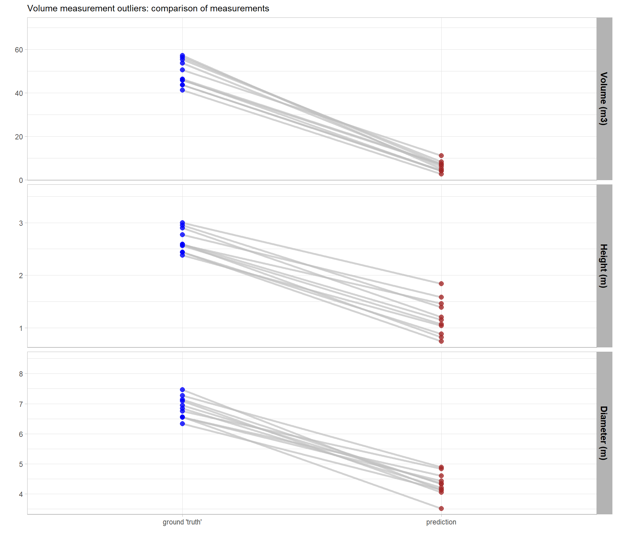
RGB with the predicted piles (brown) and the ground-truth piles (blue)
# nrow(bad_vol_df_temp)
# plot RGB
plts_temp <-
  1:nrow(bad_vol_df_temp) %>%
  # .[1] %>%
  purrr::map(function(x){
    dta <- bad_vol_df_temp %>% dplyr::slice(x)
    gt <- pj_slash_piles_polys %>% dplyr::filter(pile_id==dta$pile_id)
    pr <- final_predicted_slash_piles %>% dplyr::filter(pred_id==dta$pred_id)
    #plt
    ortho_plt_fn(my_ortho_rast=pj_rgb_rast, stand=sf::st_union(gt,pr), buffer=6) +
      ggplot2::geom_sf(data = gt, fill = NA, color = "blue", lwd = 0.6) +
      ggplot2::geom_sf(data = pr, fill = NA, color = "brown", lwd = 0.5)
  })
# plts_temp
# combine
patchwork::wrap_plots(
  plts_temp
  , ncol = 4
)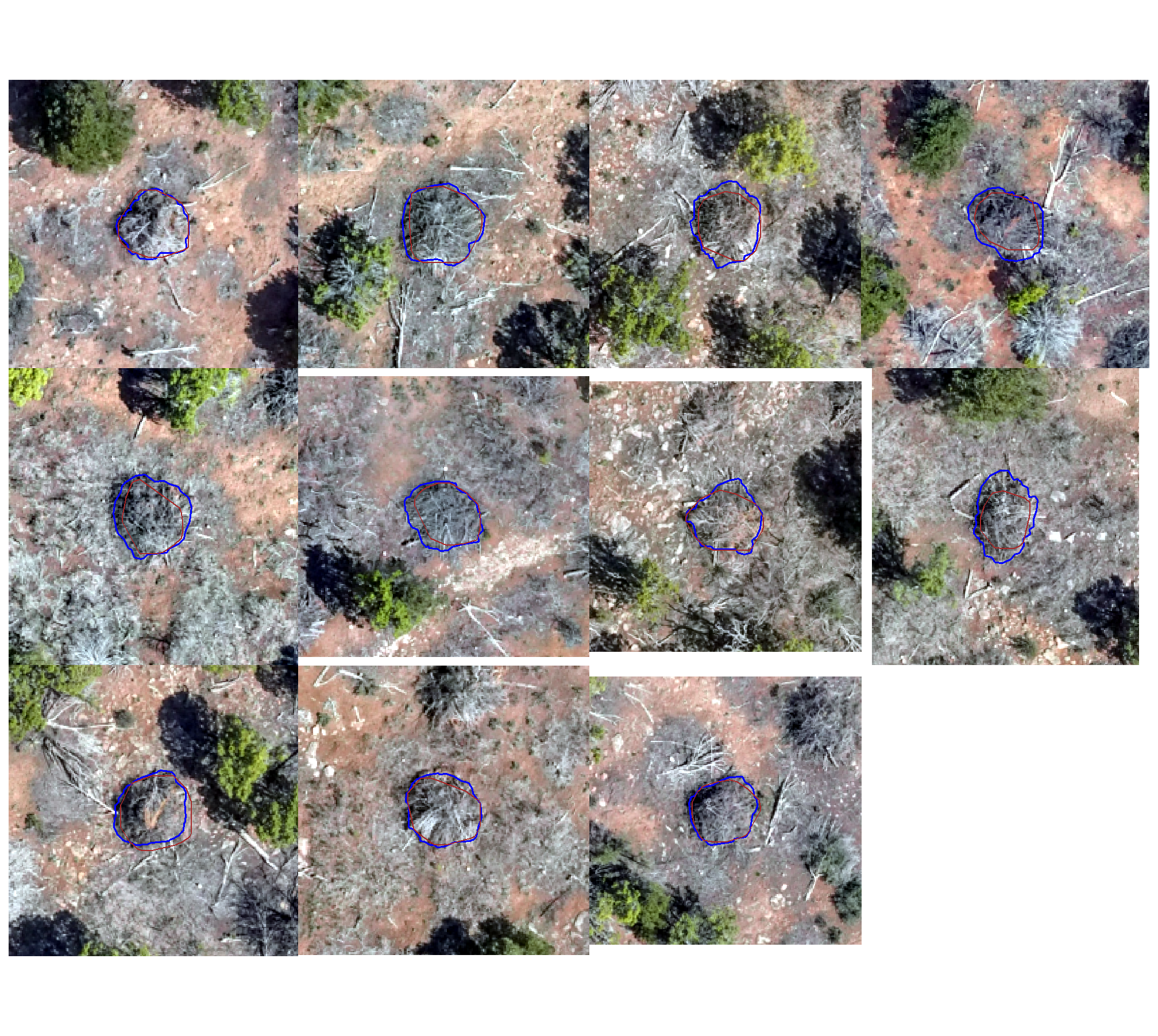
just looking at the RGB, the pile footprints are in good alignment
let’s look at the CHM
# cloud2raster_ans$chm_rast %>%
#   terra::clamp(upper = structural_params_settings$max_ht_m, lower = 0, values = F) %>%
#   terra::plot()
# bad_vol_df_temp %>% dplyr::glimpse()
# plot RGB + CHM
plts_temp <-
  1:nrow(bad_vol_df_temp) %>%
  # sample(1) %>%
  purrr::map(function(x){
    dta <- bad_vol_df_temp %>% dplyr::slice(x)
    gt <- pj_slash_piles_polys %>% dplyr::filter(pile_id==dta$pile_id)
    pr <- final_predicted_slash_piles %>% dplyr::filter(pred_id==dta$pred_id)
    #plt
    ortho_plt_fn(my_ortho_rast=pj_rgb_rast, stand=sf::st_union(gt,pr), buffer=6) +
      ggnewscale::new_scale_fill() +
      ggplot2::geom_tile(
        data = cloud2raster_ans$chm_rast %>%
          terra::crop(
            sf::st_union(gt,pr) %>%
              sf::st_transform(terra::crs(cloud2raster_ans$chm_rast)) %>%
              terra::vect()
          ) %>%
          terra::mask(
            sf::st_union(gt,pr) %>%
              sf::st_transform(terra::crs(cloud2raster_ans$chm_rast)) %>%
              terra::vect()
          ) %>%
          # slice the chm below our desired height
          # this is what slash_pile_detect_watershed() does
          terra::clamp(upper = 2.3, lower = 0, values = F) %>%
          terra::as.data.frame(xy=T) %>%
          dplyr::rename(f=3)
        , mapping = ggplot2::aes(x=x,y=y,fill=f)
        , alpha = 0.5
      ) +
      ggplot2::scale_fill_viridis_c(option = "plasma", na.value = "gray",name = "CHM (m)") +
      ggplot2::geom_sf(data = gt, fill = NA, color = "blue", lwd = 0.6) +
      ggplot2::geom_sf(data = pr, fill = NA, color = "brown", lwd = 0.5) +
      ggplot2::labs(
        subtitle = paste0(
          "GT ht: ", round(dta$gt_height_m,1)
          , " | Pred ht: ", round(dta$pred_height_m,1)
          , "\nGT dia: ", round(dta$gt_diameter_m,1)
          , " | Pred dia: ", round(dta$pred_diameter_m,1)
        )
      ) +
      ggplot2::theme(legend.text = ggplot2::element_text(size = 6),legend.title = ggplot2::element_text(size = 6))
  })
# plts_temp
# combine
patchwork::wrap_plots(
  plts_temp
  , ncol = 3
)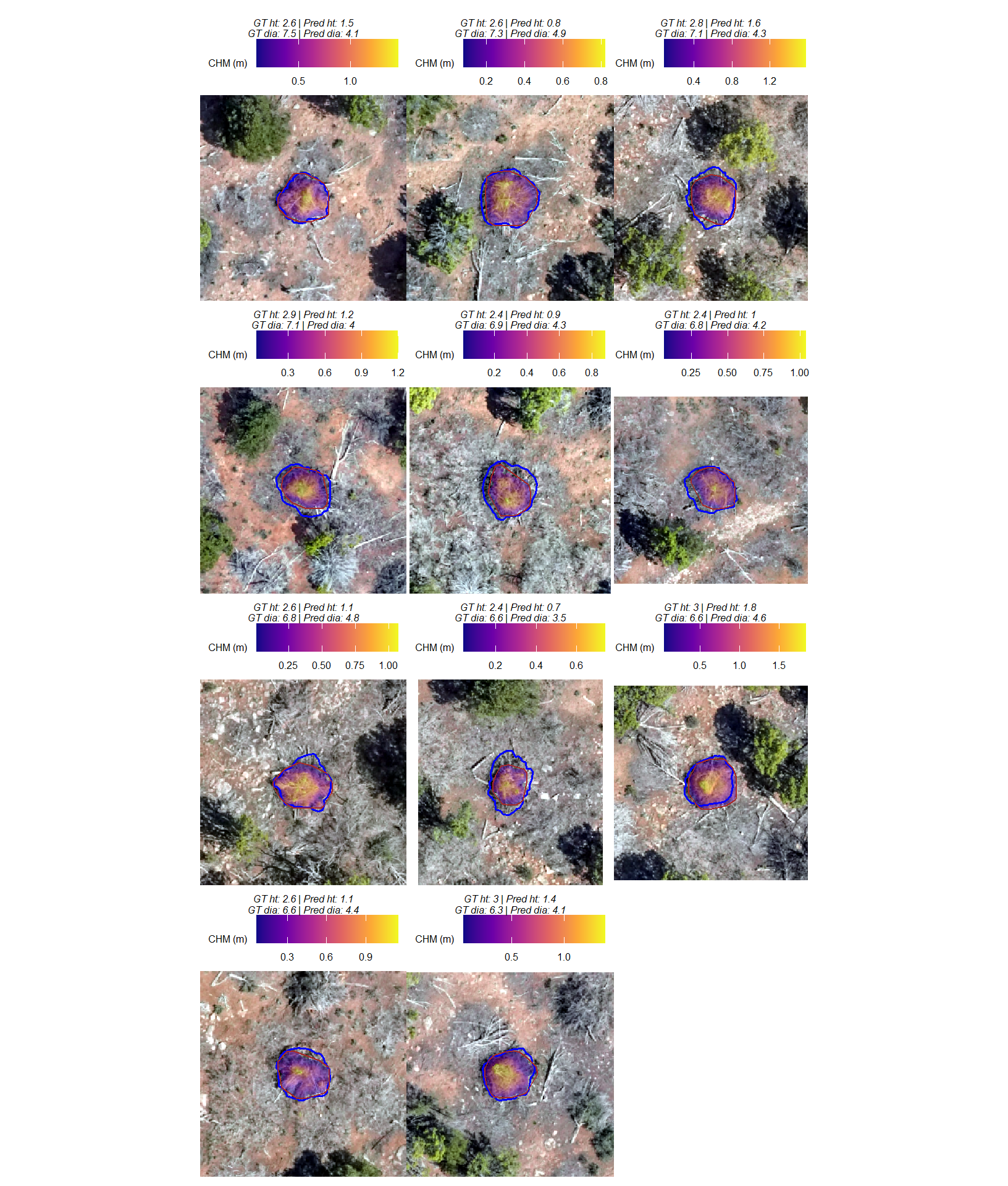
The issue here is not with the specific height slice of the CHM based on the max_ht_m parameter as we saw with the training data pile volume comparison. Instead, the issue is the field-measured height and diameter
10.4.6 Stand-level Aggregation
before we leave, let’s summarize the measurement values of the predictions (true positive and false positive) and the ground truth data (true positive and false negative) over the entire stand (this is similar to a basal area comparison in a forest inventory)
sum_df_temp <-
  ground_truth_prediction_match_ans %>%
  dplyr::ungroup() %>%
  dplyr::select(-c(pred_id)) %>%
  dplyr::summarise(
    dplyr::across(
      .cols = tidyselect::starts_with("gt_") | tidyselect::starts_with("pred_")
      , ~sum(.x,na.rm=T)
    )
  ) %>%
  tidyr::pivot_longer(
    cols = dplyr::everything()
    , names_to = "metric"
    , values_to = "value"
  ) %>%
  dplyr::mutate(
    which_data = dplyr::case_when(
        stringr::str_starts(metric,"gt_") ~ "ground truth"
        , stringr::str_starts(metric,"pred_") ~ "prediction"
        , T ~ "error"
      ) %>%
      ordered()
    , pile_metric = metric %>%
      stringr::str_remove("(_rmse|_rrmse|_mean|_mape)$") %>%
      stringr::str_extract("(paraboloid_volume|volume|area|height|diameter)") %>%
      factor(
        ordered = T
        , levels = c(
          "height"
          , "diameter"
          , "area"
          , "volume"
          , "paraboloid_volume"
        )
        , labels = c(
          "Height (m)"
          , "Diameter (m)"
          , "Area (m2)"
          , "Volume (m3)"
          , "Volume paraboloid"
        )
      )
  ) %>%
  dplyr::group_by(pile_metric) %>%
  dplyr::arrange(pile_metric,which_data) %>%
  dplyr::mutate(
    pct_diff = (value-dplyr::lag(value))/dplyr::lag(value)
  ) %>%
  dplyr::ungroup()
plot
# plot it
sum_df_temp %>%
  dplyr::ungroup() %>%
  dplyr::mutate(
    stand_id=1
    , lab = paste0(
      scales::comma(value,accuracy=0.1)
      , dplyr::case_when(
        is.na(pct_diff) ~ ""
        , T ~ paste0(
          "\n"
          , ifelse(pct_diff<0,"-","+")
          ,scales::percent(abs(pct_diff),accuracy=0.1)
        )
      )
    )
  ) %>%
  ggplot2::ggplot(
    mapping = ggplot2::aes(
      x = which_data
      , y = value
      , label = lab
      , group = stand_id
    )
  ) +
  ggplot2::geom_line(key_glyph = "point", alpha = 0.7, color = "gray", lwd = 1.1) +
  ggplot2::geom_col(mapping = ggplot2::aes(fill = which_data), alpha = 1, width = 0.4) +
  ggplot2::scale_color_manual(values = c("blue","brown")) +
  ggplot2::scale_fill_manual(values = c("blue","brown")) +
  ggplot2::geom_text(
    vjust = -0.25
  ) +
  ggplot2::facet_grid(rows = dplyr::vars(pile_metric), scales = "free_y", axes = "all_x") +
  ggplot2::scale_y_continuous(labels = scales::comma, expand = ggplot2::expansion(mult = c(0,.3)), breaks = NULL) +
  ggplot2::labs(
    x = "", y = "", color = ""
    , subtitle = "Comparison of aggregated measurements at the stand level"
  ) +
  ggplot2::theme_light() +
  ggplot2::theme(
    legend.position = "none"
    , axis.text.x = ggplot2::element_text(size = 11, color = "black", face = "bold")
    , strip.text = ggplot2::element_text(size = 11, color = "black", face = "bold")
    , panel.grid = ggplot2::element_blank()
) 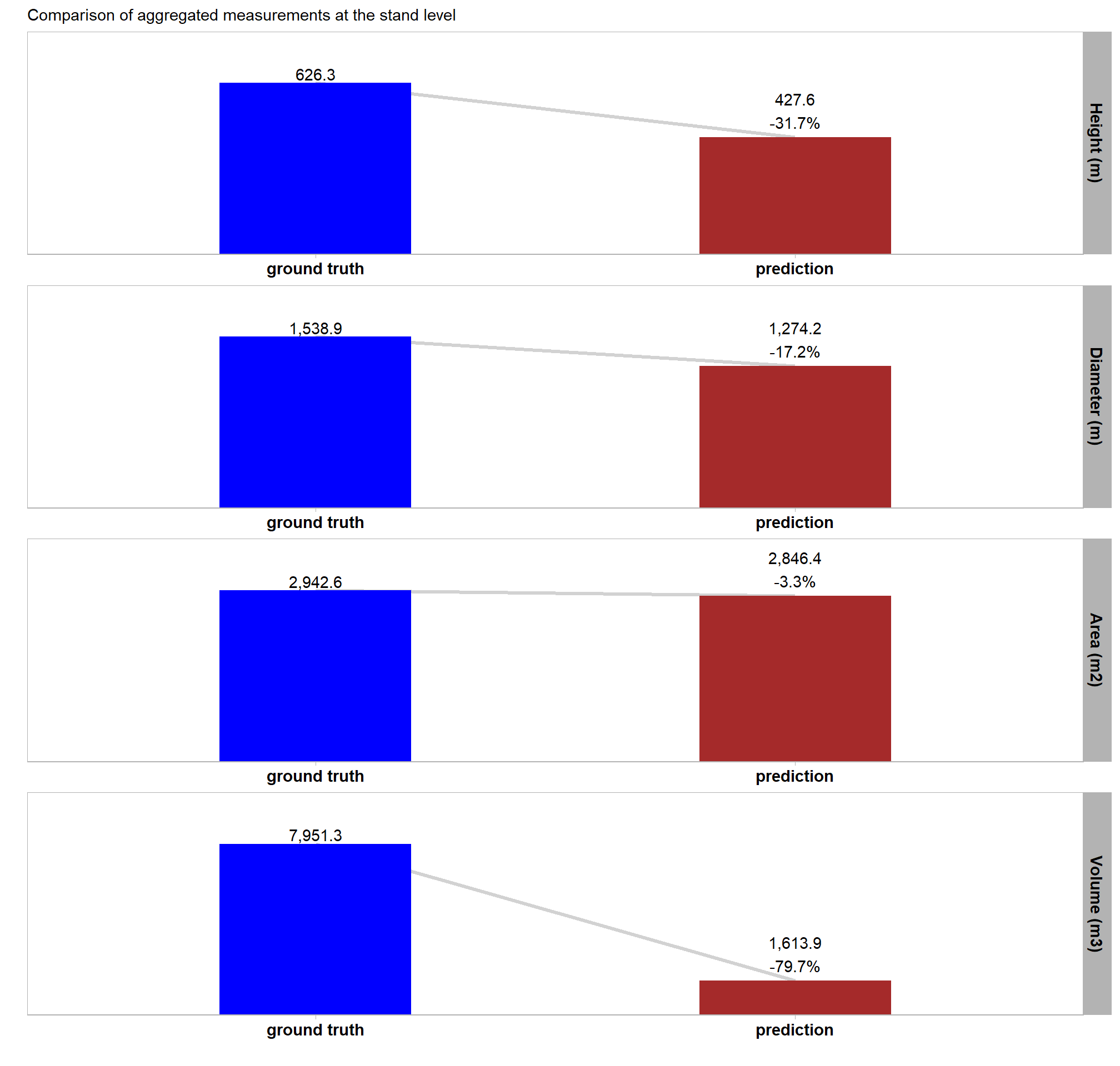
table it
sum_df_temp %>%
  dplyr::select(pile_metric, which_data, value, pct_diff) %>%
  dplyr::mutate(
    value = scales::comma(value,accuracy=0.1)
    , pct_diff = scales::percent(pct_diff,accuracy=0.1)
  ) %>%
  kableExtra::kbl(
    caption = "Comparison of aggregated measurements at the stand level"
    , col.names = c(
      ".", "measurement source"
      , "stand-level total", "% difference"
    )
    , escape = F
  ) %>%
  kableExtra::kable_styling() %>%
kableExtra::collapse_rows(columns = 1, valign = "top")| . | measurement source | stand-level total | % difference |
|---|---|---|---|
| Height (m) | ground truth | 626.3 | NA |
| prediction | 427.6 | -31.7% | |
| Diameter (m) | ground truth | 1,538.9 | NA |
| prediction | 1,274.2 | -17.2% | |
| Area (m2) | ground truth | 2,942.6 | NA |
| prediction | 2,846.4 | -3.3% | |
| Volume (m3) | ground truth | 7,951.3 | NA |
| prediction | 1,613.9 | -79.7% |
10.5 Pile Detection: Structural Only
we’ll now detail the parameterization of the methodology using structural (CHM data) only as if no spectral data were available. This setup will allow us to compare it with the data fusion approach we reviewed above. Essentially, the availability of complementary spectral data permits the use of more relaxed size and structural thresholds. Conversely, when working exclusively with structural data, users are advised to employ more restrictive structural filters to effectively suppress false positives and ensure reliable pile detection.
10.5.1 Structural Detection
we’re going to set the four structural parameters (max_ht_m, max_area_m2, convexity_pct, circle_fit_iou_pct) of the slash_pile_detect_watershed() function (defined here) which are used to determine candidate slash piles from the CHM data alone based on our expectations from the treatment prescription and it’s implementation on the ground. Our settings here will be more restrictive in an attempt to suppress false positives which we do not have the benefit of filtering out using spectral data.
the treatment prescription for the unit of interest called for thinning to create a residual structure with “uniform gaps between trees” with via a “heavy intensity thinning” that called for gaps of “at least Based on the prescription and anecdotal feedback, the following parameter settings will be used:
- max_ht_m: This parameter will be set to 1.8 m (5.9 feet). This represents a 20% increase over the 1.5 m (5 ft) minimum height specified in the prescription, to account for the feedback that piles were larger than expected.
- min_ht_m: This parameter will be set to 0.6 m (2 foot). This creates a 1.2 m (3.9 feet) vertical range for structural detection. This setting allows for the acceptance of piles up to 0.9 m (3 feet) smaller than the prescribed minimum of 1.5 m to account for variation in construction from the prescription and the settling of pile form over time
- min_area_m2: This parameter will be set to 2.0 square meters (21.5 square feet). This provides a small buffer below the prescribed 2.3 square meters (25 square feet) minimum area to account for minor segmentation errors or slight settling of the pile, without deviating significantly from the horizontal prescription.
- max_area_m2: This parameter will be set to 15 square meters (161.5 square feet). This represents a nearly seven-fold increase compared to the 2.3 square meters minimum. The rationale for this significant increase compared to the upper height threshold is because it is physically easier to construct piles that are wider and more irregular in the horizontal direction than the vertical direction.
- convexity_pct: To account for the “messy” and irregularly shaped piles, this parameter will be set to 0.12 which is in the the optimal range identified in the Ponderosa Pine training data based on predictions for structural only input data
- circle_fit_iou_pct: This parameter will be set to 0.39, which is approximately 8 percentage points lower than the optimal value identified in the Ponderosa Pine training data. This value is used in conjunction with convexity_pct to allow for a wider range of non-circular, irregular shapes
- CHM Resolution (chm_res_m): A 0.1 m (0.33 feet, 3.9 inches) CHM raster will be used. This fine resolution will enhance the granular distinction between piles and lower tree branches which is important given the close proximity of piles to residual trees noted by managers
slash_pile_detect_watershed() that CHM
outdir_temp <- "../data/Dawson_data"
fnm_temp <- file.path(outdir_temp,"pj_structural_only_predictions.gpkg")
# "new_pj_structural_candidate_segments.gpkg" = convexity_pct = 0.06; circle_fit_iou_pct = 0.35
if(!file.exists(fnm_temp)){
  set.seed(88)
  structural_final_predicted_slash_piles <- slash_pile_detect_watershed(
    chm_rast = chm_rast_stand
    #### height and area thresholds for the detected piles
    # these should be based on data from the literature or expectations based on the prescription
    , max_ht_m = 1.8 # set the max expected pile height
    , min_ht_m = 0.6 # set the min expected pile height
    , min_area_m2 = 2.0 # set the min expected pile area
    , max_area_m2 = 15 # set the max expected pile area
    #### irregularity filtering
    # 1 = perfectly convex (no inward angles); 0 = so many inward angles
    # values closer to 1 remove more irregular segments;
      # values closer to 0 keep more irregular segments (and also regular segments)
    # these will all be further filtered for their circularity and later smoothed to remove blocky edges
    # and most inward angles by applying a convex hull to the original detected segment
    , convexity_pct = 0.12 # min required overlap between the predicted pile and the convex hull of the predicted pile
    #### circularity filtering
    # 1 = perfectly circular; 0 = not circular (e.g. linear) but also circular
    # min required IoU between the predicted pile and the best fit circle of the predicted pile
    , circle_fit_iou_pct = 0.39
    #### shape refinement & overlap removal
    ## smooth_segs = T ... convex hulls of raster detected segments are returned, any that overlap are removed
    ## smooth_segs = F ... raster detected segments are returned (blocky) if they meet all prior rules
    , smooth_segs = T
  )
  # save
  structural_final_predicted_slash_piles %>% sf::st_write(fnm_temp, append = F)
}else{
  structural_final_predicted_slash_piles <- sf::st_read(fnm_temp, quiet=T)
}
# what did we get?
structural_final_predicted_slash_piles %>% dplyr::glimpse()
## Rows: 325
## Columns: 8
## $ pred_id <int> 1, 6, 7, 8, 10, 11, 12, 13, 14, 15, 16, 17, 18, 19, 20…
## $ area_m2 <dbl> 12.410, 3.500, 11.255, 11.680, 6.810, 12.075, 2.875, 3…
## $ volume_m3 <dbl> 7.611119, 2.956290, 5.879869, 7.763583, 7.834494, 7.48…
## $ max_height_m <dbl> 1.500000, 1.800000, 1.800000, 1.800000, 1.800000, 1.80…
## $ volume_per_area <dbl> 0.6133054, 0.8446542, 0.5224228, 0.6646903, 1.1504396,…
## $ pct_chull <dbl> 0.7687349, 0.8142857, 0.8573967, 0.8672945, 0.7239354,…
## $ diameter_m <dbl> 5.223983, 2.657066, 4.100000, 4.438468, 3.448188, 5.85…
## $ geom <POLYGON [m]> POLYGON ((707989.7 4193402,..., POLYGON ((7082…CHM with the structural-only predicted piles (brown) and the ground-truth piles (blue)
chm_rast_stand %>%
  terra::aggregate(fact = 2, na.rm=T) %>%  #, fun = "median", cores = lasR::half_cores(), na.rm = T) %>%
  terra::plot(col = viridis::plasma(100), axes = F)
  terra::plot(
    pj_stand_boundary %>%
      terra::vect() %>%
      terra::project(terra::crs(cloud2raster_ans$chm_rast))
    , add = T, border = "black", col = NA, lwd = 1.2
  )
  terra::plot(
    pj_slash_piles_polys %>%
      terra::vect() %>%
      terra::project(terra::crs(cloud2raster_ans$chm_rast))
    , add = T, border = "blue", col = NA, lwd = 1.2
  )
  terra::plot(
    structural_final_predicted_slash_piles %>%
      terra::vect() %>%
      terra::project(terra::crs(cloud2raster_ans$chm_rast))
    , add = T, border = "brown", col = NA, lwd = 1.3
  )
let’s focus in on a specific area to plot the ground truth and the predicted piles overlaid on the RGB
# all gt piles that intersect
gt_temp <- pj_slash_piles_polys %>%
  dplyr::inner_join(
    pj_slash_piles_polys %>%
      sf::st_transform(sf::st_crs(aoi_for_plt)) %>%
      sf::st_intersection(aoi_for_plt) %>%
      sf::st_drop_geometry() %>%
      dplyr::select(pile_id)
  ) %>%
  sf::st_transform(sf::st_crs(aoi_for_plt))
# all pred piles that intersect
pred_temp <- structural_final_predicted_slash_piles %>%
  dplyr::inner_join(
    structural_final_predicted_slash_piles %>%
      sf::st_intersection(aoi_for_plt) %>%
      sf::st_drop_geometry() %>%
      dplyr::select(pred_id)
  )
# plot it
ortho_plt_temp <-
  ortho_plt_fn(
    my_ortho_rast = pj_rgb_rast
    , stand = aoi_for_plt
    , buffer = 5
  )
# ortho_plt_temp
plot a sample of the RGB with the predicted piles (brown) and the ground-truth piles (blue)
ortho_plt_temp +
  # ggplot2::ggplot() +
  ggplot2::geom_sf(
    data = gt_temp
    , color = "blue"
    , fill = NA
    , lwd = 1
  ) +
  ggplot2::geom_sf(
    data = pred_temp
    , color = "brown"
    , fill = NA
    , lwd = 1
  ) +
  ggplot2::theme_void() +
  ggplot2::theme(legend.position = "none")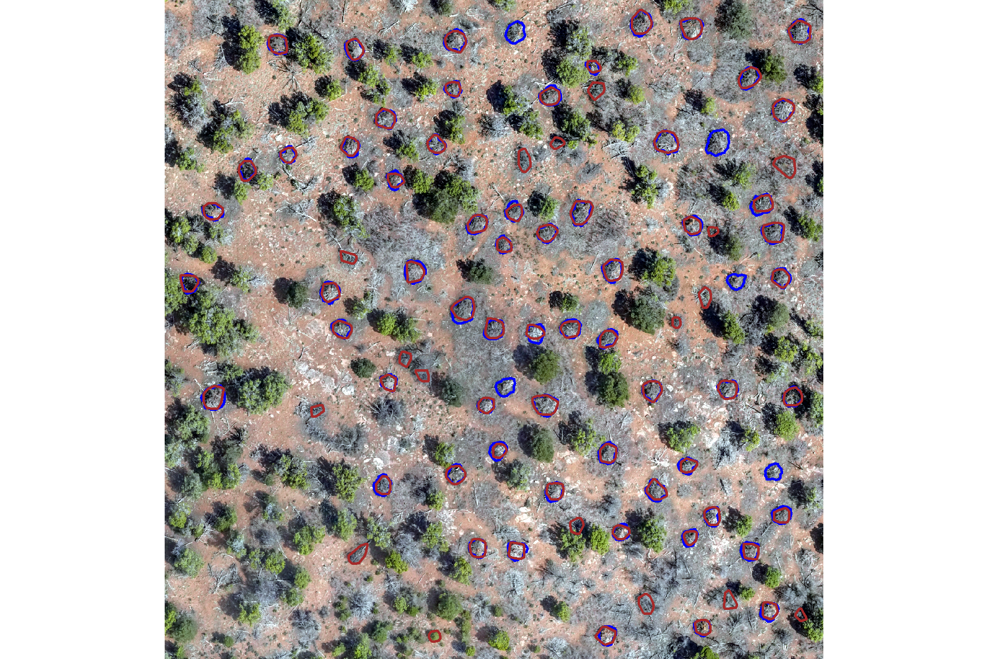
plot the same sample of the CHM with the predicted piles (brown) and the ground-truth piles (blue)
cloud2raster_ans$chm_rast %>%
  terra::crop(aoi_for_plt %>% terra::vect() %>% terra::project(cloud2raster_ans$chm_rast)) %>%
  terra::mask(aoi_for_plt %>% terra::vect() %>% terra::project(cloud2raster_ans$chm_rast)) %>%
  terra::aggregate(fact = 2, na.rm=T) %>%  #, fun = "median", cores = lasR::half_cores(), na.rm = T) %>%
  terra::plot(col = viridis::plasma(100), axes = F)
  terra::plot(
    gt_temp %>%
      terra::vect() %>%
      terra::project(terra::crs(cloud2raster_ans$chm_rast))
    , add = T, border = "blue", col = NA, lwd = 1.2
  )
  terra::plot(
    pred_temp %>%
      terra::vect() %>%
      terra::project(terra::crs(cloud2raster_ans$chm_rast))
    , add = T, border = "brown", col = NA, lwd = 1.3
  )
10.5.2 Detection and Quantification Accuracy
let’s see how we did given the list of predictions compared to the ground truth data using the confusion matrix matching process we outlined in this earlier section.
we’ll filter both ground truth and predicted piles to keep only those that actually intersect with the study unit boundary for comparison
# add filter
# pred
structural_final_predicted_slash_piles <- structural_final_predicted_slash_piles %>%
  dplyr::left_join(
    structural_final_predicted_slash_piles %>%
      sf::st_intersection(
        pj_stand_boundary %>%
          sf::st_transform(sf::st_crs(structural_final_predicted_slash_piles))
      ) %>%
      sf::st_drop_geometry() %>%
      dplyr::distinct(pred_id) %>%
      dplyr::mutate(is_in_stand=T)
    , by = "pred_id"
  ) %>%
  dplyr::mutate(is_in_stand=dplyr::coalesce(is_in_stand, F))
10.5.2.1 Instance matching
now apply the instance matching process we outlined in this earlier section to establish True Positives (TP), False Positives (FP, commissions), and False Negatives (FN, omissions)
# ground truth and prediction matching process
structural_ground_truth_prediction_match_ans <- ground_truth_prediction_match(
  ground_truth =
    pj_slash_piles_polys %>%
    dplyr::filter(is_in_stand) %>%
    dplyr::arrange(desc(field_diameter_m)) %>%
    sf::st_transform(sf::st_crs(structural_final_predicted_slash_piles))
  , gt_id = "pile_id"
  , predictions = structural_final_predicted_slash_piles %>% dplyr::filter(is_in_stand)
  , pred_id = "pred_id"
  , min_iou_pct = 0.05
)
# add data from gt and pred piles
structural_ground_truth_prediction_match_ans <-
  structural_ground_truth_prediction_match_ans %>%
  # add area of gt
  dplyr::left_join(
    pj_slash_piles_polys %>%
      sf::st_drop_geometry() %>%
      dplyr::filter(is_in_stand) %>%
      dplyr::select(
        pile_id
        , image_gt_area_m2
        , image_gt_diameter_m
        , field_gt_volume_m3
        , height_m
        , field_diameter_m
      ) %>%
      dplyr::rename(
        gt_height_m = height_m
        , gt_diameter_m = field_diameter_m
        , gt_area_m2 = image_gt_area_m2
        , gt_volume_m3 = field_gt_volume_m3
      ) %>%
      dplyr::mutate(pile_id=as.numeric(pile_id))
    , by = "pile_id"
  ) %>%
  # add info from predictions
  dplyr::left_join(
    structural_final_predicted_slash_piles %>%
      sf::st_drop_geometry() %>%
      dplyr::select(
        pred_id
        , area_m2, volume_m3, max_height_m, diameter_m
      ) %>%
      dplyr::rename(
        pred_area_m2 = area_m2, pred_volume_m3 = volume_m3
        , pred_height_m = max_height_m, pred_diameter_m = diameter_m
      )
    , by = dplyr::join_by(pred_id)
  ) %>%
  dplyr::mutate(
    ### calculate these based on the formulas below...agg_ground_truth_match() depends on those formulas
    # ht diffs
    diff_height_m = pred_height_m-gt_height_m
    , pct_diff_height_m = (gt_height_m-pred_height_m)/gt_height_m
    # diameter
    , diff_field_diameter_m = pred_diameter_m-gt_diameter_m
    , pct_diff_field_diameter_m = (gt_diameter_m-pred_diameter_m)/gt_diameter_m
    # image diameter
    , diff_image_diameter_m = pred_diameter_m-image_gt_diameter_m
    , pct_diff_image_diameter_m = (image_gt_diameter_m-pred_diameter_m)/image_gt_diameter_m
    # area diffs
    , diff_area_m2 = pred_area_m2-gt_area_m2
    , pct_diff_area_m2 = (gt_area_m2-pred_area_m2)/gt_area_m2
    # # volume diffs
    # , diff_image_volume_m3 = pred_volume_m3-image_gt_volume_m3
    # , pct_diff_image_volume_m3 = (image_gt_volume_m3-pred_volume_m3)/image_gt_volume_m3
    # , diff_field_volume_m3 = pred_volume_m3-field_gt_volume_m3
    # , pct_diff_field_volume_m3 = (field_gt_volume_m3-pred_volume_m3)/field_gt_volume_m3
  )
# huh?
structural_ground_truth_prediction_match_ans %>% dplyr::glimpse()
## Rows: 339
## Columns: 23
## $ pile_id <dbl> 156, 73, 137, 249, 85, 247, 174, 149, 218, 7…
## $ i_area <dbl> 10.753418, 13.624855, 11.746210, 9.142921, 1…
## $ u_area <dbl> 11.929006, 17.953926, 15.612023, 12.799369, …
## $ iou <dbl> 0.9014513, 0.7588789, 0.7523823, 0.7143259, …
## $ pred_id <int> 80, 202, 68, 144, 273, 218, 214, 233, 213, 1…
## $ match_grp <ord> true positive, true positive, true positive,…
## $ gt_area_m2 <dbl> 11.112424, 17.303781, 15.228233, 12.767290, …
## $ image_gt_diameter_m <dbl> 4.096896, 5.230641, 5.228979, 4.778329, 4.77…
## $ gt_volume_m3 <dbl> 56.38418, 45.20433, 55.45441, 57.24669, 46.1…
## $ gt_height_m <dbl> 2.58, 2.19, 2.77, 2.90, 2.44, 2.38, 2.56, 2.…
## $ gt_diameter_m <dbl> 7.46, 7.25, 7.14, 7.09, 6.94, 6.84, 6.75, 6.…
## $ pred_area_m2 <dbl> 11.570, 14.275, 12.130, 9.175, 10.180, 9.930…
## $ pred_volume_m3 <dbl> 7.240877, 7.230272, 8.337802, 5.046406, 4.14…
## $ pred_height_m <dbl> 1.46, 1.08, 1.58, 1.20, 0.88, 1.04, 1.07, 1.…
## $ pred_diameter_m <dbl> 4.123106, 5.420332, 4.326662, 4.049691, 4.34…
## $ diff_height_m <dbl> -1.12, -1.11, -1.19, -1.70, -1.56, -1.34, -1…
## $ pct_diff_height_m <dbl> 0.4341085, 0.5068493, 0.4296029, 0.5862069, …
## $ diff_field_diameter_m <dbl> -3.336894, -1.829668, -2.813338, -3.040309, …
## $ pct_diff_field_diameter_m <dbl> 0.4473049, 0.2523680, 0.3940250, 0.4288165, …
## $ diff_image_diameter_m <dbl> 0.02620980, 0.18969070, -0.90231755, -0.7286…
## $ pct_diff_image_diameter_m <dbl> -0.006397478, -0.036265286, 0.172560942, 0.1…
## $ diff_area_m2 <dbl> 0.45757578, -3.02878145, -3.09823340, -3.592…
## $ pct_diff_area_m2 <dbl> -0.041176954, 0.175035813, 0.203453238, 0.28…that’s a lot of great detail at the individual pile instance level for us to dig into. before we do that, let’s aggregate the instances to see how we did at the stand level overall
10.5.2.2 Overall (stand level)
Now we’ll aggregate the instance matching results to calculate overall performance assessment metrics. Here, we take the counts of True Positives (TP), False Positives (FP, commissions), and False Negatives (FN, omissions), to determine overall accuracy. This aggregation will give us two types of results:
detection accuracy metrics: such as Recall, Precision, and F-score, are calculated directly by aggregating these raw TP, FP, and FN counts and quantifies the method’s ability to find the piles
quantification accuracy metrics: such as RMSE, MAPE, and Mean Error of pile form measurements (e.g. height, diameter) are calculated by aggregating the differences between the estimated pile attributes and the ground truth values for instances classified as True Positives. These metrics tell us about the method’s ability to accurately quantify the form of the piles it successfully identified
structural_agg_ground_truth_match_ans <- agg_ground_truth_match(ground_truth_prediction_match_ans = structural_ground_truth_prediction_match_ans)
# huh?
structural_agg_ground_truth_match_ans %>% dplyr::glimpse()
## Rows: 1
## Columns: 20
## $ tp_n <dbl> 236
## $ fp_n <dbl> 62
## $ fn_n <dbl> 41
## $ omission_rate <dbl> 0.1480144
## $ commission_rate <dbl> 0.2080537
## $ precision <dbl> 0.7919463
## $ recall <dbl> 0.8519856
## $ f_score <dbl> 0.8208696
## $ diff_area_m2_rmse <dbl> 1.791876
## $ diff_field_diameter_m_rmse <dbl> 1.78518
## $ diff_height_m_rmse <dbl> 1.21531
## $ diff_image_diameter_m_rmse <dbl> 0.406211
## $ diff_area_m2_mean <dbl> -1.14091
## $ diff_field_diameter_m_mean <dbl> -1.704
## $ diff_height_m_mean <dbl> -1.188069
## $ diff_image_diameter_m_mean <dbl> -0.2504122
## $ pct_diff_area_m2_mape <dbl> 0.1364955
## $ pct_diff_field_diameter_m_mape <dbl> 0.3052607
## $ pct_diff_height_m_mape <dbl> 0.5192491
## $ pct_diff_image_diameter_m_mape <dbl> 0.0746874notice how there is only one row for the single stand we had ground truth data for to evaluate our method against
let’s table the most relevant metrics
structural_agg_ground_truth_match_ans %>%
  kbl_agg_gt_match(
    caption = "pile detection and form quantification accuracy metrics<br>structural only pinyon-juniper validation site"
)| . | value | |
|---|---|---|
| Detection Count | TP | 236 |
| FN | 41 | |
| FP | 62 | |
| Detection | F-score | 82% |
| Recall | 85% | |
| Precision | 79% | |
| Area m2 | ME | -1.14 |
| RMSE | 1.8 | |
| MAPE | 14% | |
| Diameter m (field) | ME | -1.70 |
| RMSE | 1.8 | |
| MAPE | 31% | |
| Diameter m (image) | ME | -0.25 |
| RMSE | 0.4 | |
| MAPE | 7% | |
| Height m | ME | -1.19 |
| RMSE | 1.2 | |
| MAPE | 52% |