Section 9 CHM Raster Resolution Testing
In this prior section we demonstrated how to use cloud2trees::cloud2raster() to process the raw point cloud data to generate the CHM (a DSM with the ground removed) for our raster-based watershed segmentation methodology. The cloud2trees package makes it easy to process raw point cloud data to generate a CHM at practically any resolution from coarse to fine grain. We performed sensitivity testing of our slash pile detection method using only a single CHM raster resolution. What is the influence of different raster resolution on the ability of the method to accurately detect and quantify piles?
9.1 Process Raw Point Cloud
We’ll use cloud2trees::cloud2raster() to process the raw point cloud data to generate a set of CHM rasters at varying resolutions
chm_res_list <- seq(from=0.10,to=0.50,by=0.05)
# process point clouds
chm_res_list %>%
  purrr::map(function(chm_res_m){
    message(paste0("CHMing...........",chm_res_m))
    dir_temp <- paste0("../data/point_cloud_processing_delivery_chm",chm_res_m,"m")
    # do it
    if(!dir.exists(dir_temp)){
      # cloud2trees
      cloud2raster_ans <- cloud2trees::cloud2raster(
        output_dir = "../data"
        , input_las_dir = "f:\\PFDP_Data\\p4pro_images\\P4Pro_06_17_2021_half_half_optimal\\2_densification\\point_cloud"
        , accuracy_level = 2
        , keep_intrmdt = T
        , dtm_res_m = 0.25
        , chm_res_m = chm_res_m
        , min_height = 0 # effectively generates a DSM based on non-ground points
      )
      # rename
      file.rename(from = "../data/point_cloud_processing_delivery", to = dir_temp)
    }
  })
# which dirs?
chm_res_list[
  chm_res_list %>%
    purrr::map(~paste0("../data/point_cloud_processing_delivery_chm",.x,"m")) %>%
    unlist() %>%
    dir.exists()
]
9.2 Structural Only: Parameter Testing
we could simply map these combinations over our slash_pile_detect_watershed() function but that would entail performing the same action multiple times. we defined a specialized function to efficiently map over all of these combinations in this section which we’ll just load now.
# we defined a specialized function to efficiently map over all of these combinations
source("_utils_parameter_combo_testing.R")
# lower level functions used in slash_pile_detect_watershed()
source("_utils_slash_pile_detect.R")
let’s test different parameter combinations of our watershed segmentation, rules-based slash pile detection methodology for each CHM raster resolution from more coarse, to finer resolution
param_combos_df <-
  tidyr::crossing(
    max_ht_m = seq(from = 2, to =  5, by = 1) # set the max expected pile height (could also do a minimum??)
    , min_area_m2 = c(2) # seq(from = 1, to =  2, by = 1) # set the min expected pile area
    , max_area_m2 = seq(from = 10, to =  100, by = 10) # set the max expected pile area
    , convexity_pct = seq(from = 0.3, to =  0.8, by = 0.1) # min required overlap between the predicted pile and the convex hull of the predicted pile
    , circle_fit_iou_pct = seq(from = 0.3, to = 0.8, by = 0.1)
  ) %>%
  dplyr::mutate(rn = dplyr::row_number()) %>%
  dplyr::relocate(rn)
# how many combos are we testing?
n_combos_tested_chm <- nrow(param_combos_df) #combos per chm
n_combos_tested <- length(chm_res_list)*n_combos_tested_chm #combos overall structural only
# there are 5 spectral_weight settings + no spectral data (spectral_weight=0) = 6
spectral_settings_tested <- 6
# how many combos overall is this for the spectral testing?
n_combos_tested_spectral <- n_combos_tested*spectral_settings_tested
# how many combos PER CHM is this for the spectral testing?
n_combos_tested_spectral_chm <- n_combos_tested_chm*spectral_settings_tested
map over each CHM raster for pile detection using each of these parameter combinations
param_combos_piles_flist <- chm_res_list %>%
  purrr::map(function(chm_res_m){
    message(paste0("param_combos_piles_detect_fn...........",chm_res_m))
    # file
    f_temp <- file.path("../data",paste0("param_combos_piles_chm",chm_res_m,"m.gpkg"))
    # chm dir
    dir_temp <- paste0("../data/point_cloud_processing_delivery_chm",chm_res_m,"m")
    # chm file
    chm_f <- file.path(dir_temp, paste0("chm_", chm_res_m,"m.tif"))
    # check and do it
    if(!file.exists(f_temp) && file.exists(chm_f) ){
      # read chm
      chm_rast <- terra::rast(chm_f)
      # do it
      param_combos_piles <- param_combos_piles_detect_fn(
        chm = chm_rast %>%
          terra::crop(
            stand_boundary %>%
              dplyr::slice(1) %>%
              sf::st_buffer(5) %>%
              sf::st_transform(terra::crs(chm_rast)) %>%
              terra::vect()
          )
        , param_combos_df = param_combos_df
        , smooth_segs = T
        , ofile = f_temp
      )
      # param_combos_piles %>% dplyr::glimpse()

      # save it
      sf::st_write(param_combos_piles, f_temp, append = F, quiet = T)
      return(f_temp)
    }else if(file.exists(f_temp)){
      return(f_temp)
    }else{
      return(NULL)
    }
  })
# which successes?
param_combos_piles_flist
9.2.1 Validation over parameter combinations
now we need to validate these combinations against the ground truth data and we can map over the ground_truth_prediction_match() function to get true positive, false positive (commission), and false negative (omission) classifications for the predicted and ground truth piles
param_combos_gt_flist <- chm_res_list %>%
  purrr::map(function(chm_res_m){
    message(paste0("ground_truth_prediction_match...........",chm_res_m))
    param_combos_piles_fnm <- file.path("../data",paste0("param_combos_piles_chm",chm_res_m,"m.gpkg"))
    # file creating now
    f_temp <- file.path("../data",paste0("param_combos_gt_chm",chm_res_m,"m.csv"))
    # check
    if(!file.exists(f_temp) && file.exists(param_combos_piles_fnm)){
      # read it
      param_combos_piles <- sf::st_read(param_combos_piles_fnm)
      # do it
      param_combos_gt <-
        unique(param_combos_df$rn) %>%
        purrr::map(\(x)
          ground_truth_prediction_match(
            ground_truth = slash_piles_polys %>%
              dplyr::filter(is_in_stand) %>%
              dplyr::arrange(desc(diameter)) %>%
              sf::st_transform(sf::st_crs(param_combos_piles))
            , gt_id = "pile_id"
            , predictions = param_combos_piles %>%
              dplyr::filter(rn == x) %>%
              dplyr::filter(
                pred_id %in% (param_combos_piles %>%
                  dplyr::filter(rn == x) %>%
                  sf::st_intersection(
                    stand_boundary %>%
                      sf::st_transform(sf::st_crs(param_combos_piles))
                  ) %>%
                  sf::st_drop_geometry() %>%
                  dplyr::pull(pred_id))
              )
            , pred_id = "pred_id"
            , min_iou_pct = 0.05
          ) %>%
          dplyr::mutate(rn=x)
        ) %>%
        dplyr::bind_rows()
      # write it
      param_combos_gt %>% readr::write_csv(f_temp, append = F, progress = F)
      return(f_temp)
    }else if(file.exists(f_temp)){
      return(f_temp)
    }else{
      return(NULL)
    }
  })
# which successes?
param_combos_gt_flist
9.2.2 Aggregate Validation Metrics to Parameter Combination
now we’re going to calculate aggregated detection accuracy metrics and quantification accuracy metrics
detection accuracy metrics:
- Precision precision measures how many of the objects our method detected as slash piles were actually correct. A high precision means the method has a low rate of false alarms.
- Recall recall (i.e. detection rate) indicates how many actual (ground truth) slash piles our method successfully identified. High recall means the method is good at finding most existing piles, minimizing omissions.
- F-score provides a single, balanced measure that combines both precision and recall. A high F-score indicates overall effectiveness in both finding most piles and ensuring most detections are correct.
quantification accuracy metrics:
- Mean Error (ME) represents the direction of bias (over or under-prediction) in the original units
- RMSE represents the typical magnitude of error in the original units, with a stronger penalty for large errors
- MAPE represents the typical magnitude of error as a percentage, allowing for scale-independent comparisons
as a reminder regarding the form quantification accuracy evaluation, we will assess the method’s accuracy by comparing the true-positive matches using the following metrics:
- Volume compares the predicted volume from the irregular elevation profile and footprint to the ground truth paraboloid volume
- Diameter compares the predicted diameter (from the maximum internal distance) to the ground truth field-measured diameter.
- Area compares the predicted area from the irregular shape to the ground truth assumed circular area
- Height compares the predicted maximum height from the CHM to the ground truth field-measured height
param_combos_gt_agg_flist <- chm_res_list %>%
  purrr::map(function(chm_res_m){
    message(paste0("param_combos_gt_agg...........",chm_res_m))
    # param_combos_piles file
    param_combos_piles_fnm <- param_combos_piles_flist %>% stringr::str_subset(pattern = paste0("chm",chm_res_m,"m.gpkg")) %>% purrr::pluck(1)
    if(is.null(param_combos_piles_fnm) || !file.exists(param_combos_piles_fnm)){return(NULL)}
    # param_combos_gt file
    param_combos_gt_fnm <- param_combos_gt_flist %>% stringr::str_subset(pattern = paste0("chm",chm_res_m,"m.csv")) %>% purrr::pluck(1)
    if(is.null(param_combos_gt_fnm) || !file.exists(param_combos_gt_fnm)){return(NULL)}
    # file creating now
    f_temp <- file.path("../data",paste0("param_combos_gt_agg_chm",chm_res_m,"m.csv"))
    # check and do it
    if(!file.exists(f_temp)){
      # read param_combos_piles
      param_combos_piles <- sf::st_read(param_combos_piles_fnm)
      # read param_combos_piles
      param_combos_gt <- readr::read_csv(param_combos_gt_fnm)

      #######################################
      # let's attach a flag to only work with piles that intersect with the stand boundary
      # add in/out to piles data
      #######################################
      param_combos_piles <- param_combos_piles %>%
        dplyr::left_join(
          param_combos_piles %>%
            sf::st_intersection(
              stand_boundary %>%
                sf::st_transform(sf::st_crs(param_combos_piles))
            ) %>%
            sf::st_drop_geometry() %>%
            dplyr::select(rn,pred_id) %>%
            dplyr::mutate(is_in_stand = T)
          , by = dplyr::join_by(rn,pred_id)
        ) %>%
        dplyr::mutate(
          is_in_stand = dplyr::coalesce(is_in_stand,F)
        ) %>%
        # # get the length (diameter) and width of the polygon
        # st_bbox_by_row(dimensions = T) %>% # gets shape_length, where shape_length=length of longest bbox side
        # and paraboloid volume
        dplyr::mutate(
          # paraboloid_volume_m3 = (1/8) * pi * (shape_length^2) * max_height_m
          paraboloid_volume_m3 = (1/8) * pi * (diameter_m^2) * max_height_m
        )
      # param_combos_piles %>% dplyr::glimpse()
      #######################################
      # add data to validation
      #######################################
      param_combos_gt <-
        param_combos_gt %>%
        dplyr::mutate(pile_id = as.numeric(pile_id)) %>%
        # add area of gt
        dplyr::left_join(
          slash_piles_polys %>%
            sf::st_drop_geometry() %>%
            dplyr::select(pile_id,image_gt_area_m2,field_gt_area_m2,image_gt_volume_m3,field_gt_volume_m3,height_m,field_diameter_m) %>%
            dplyr::rename(
              gt_height_m = height_m
              , gt_diameter_m = field_diameter_m
            ) %>%
            dplyr::mutate(pile_id=as.numeric(pile_id))
          , by = "pile_id"
        ) %>%
        # add info from predictions
        dplyr::left_join(
          param_combos_piles %>%
            sf::st_drop_geometry() %>%
            dplyr::select(
              rn,pred_id
              ,is_in_stand
              , area_m2, volume_m3, max_height_m, diameter_m
              , paraboloid_volume_m3
              # , shape_length # , shape_width
            ) %>%
            dplyr::rename(
              pred_area_m2 = area_m2, pred_volume_m3 = volume_m3
              , pred_height_m = max_height_m, pred_diameter_m = diameter_m
              , pred_paraboloid_volume_m3 = paraboloid_volume_m3
            )
          , by = dplyr::join_by(rn,pred_id)
        ) %>%
        dplyr::mutate(
          is_in_stand = dplyr::case_when(
            is_in_stand == T ~ T
            , is_in_stand == F ~ F
            , match_grp == "omission" ~ T
            , T ~ F
          )
          ### calculate these based on the formulas below...agg_ground_truth_match() depends on those formulas
          # ht diffs
          , height_diff = pred_height_m-gt_height_m
          , pct_diff_height = (gt_height_m-pred_height_m)/gt_height_m
          # diameter
          , diameter_diff = pred_diameter_m-gt_diameter_m
          , pct_diff_diameter = (gt_diameter_m-pred_diameter_m)/gt_diameter_m
          # area diffs
          # , area_diff_image = pred_area_m2-image_gt_area_m2
          # , pct_diff_area_image = (image_gt_area_m2-pred_area_m2)/image_gt_area_m2
          , area_diff_field = pred_area_m2-field_gt_area_m2
          , pct_diff_area_field = (field_gt_area_m2-pred_area_m2)/field_gt_area_m2
          # volume diffs
          # , volume_diff_image = pred_volume_m3-image_gt_volume_m3
          # , pct_diff_volume_image = (image_gt_volume_m3-pred_volume_m3)/image_gt_volume_m3
          , volume_diff_field = pred_volume_m3-field_gt_volume_m3
          , pct_diff_volume_field = (field_gt_volume_m3-pred_volume_m3)/field_gt_volume_m3
          # volume diffs cone
          # # , paraboloid_volume_diff_image = pred_paraboloid_volume_m3-image_gt_volume_m3
          # , paraboloid_volume_diff_field = pred_paraboloid_volume_m3-field_gt_volume_m3
          # , pct_diff_paraboloid_volume_field = (field_gt_volume_m3-pred_paraboloid_volume_m3)/field_gt_volume_m3
        )
      #######################################
      # aggregate results from ground_truth_prediction_match()
      #######################################
      param_combos_gt_agg <- unique(param_combos_gt$rn) %>%
        purrr::map(\(x)
          agg_ground_truth_match(
            param_combos_gt %>%
              dplyr::filter(
                is_in_stand
                & rn == x
              )
          ) %>%
          dplyr::mutate(rn = x) %>%
          dplyr::select(!tidyselect::starts_with("gt_"))
        ) %>%
        dplyr::bind_rows() %>%
        # add in info on all parameter combinations
        dplyr::inner_join(
          param_combos_piles %>%
          sf::st_drop_geometry() %>%
          dplyr::distinct(
            rn,max_ht_m,min_area_m2,max_area_m2,convexity_pct,circle_fit_iou_pct
          )
          , by = "rn"
          , relationship = "one-to-one"
        )
      # write it
      param_combos_gt_agg %>% readr::write_csv(f_temp, append = F, progress = F)
      return(f_temp)
    }else if(file.exists(f_temp)){
      return(f_temp)
    }else{
      return(NULL)
    }
  })
# which successes?
param_combos_gt_agg_flist
9.3 Data Fusion: Parameter Testing
We also reviewed a data fusion approach that uses both a CHM generated from aerial point cloud data (for structural information) and RGB imagery, whereby initial candidate slash piles are first identified based on their structural form and then, filtered spectrally using the RGB imagery. We created a process to perform this filtering which takes as input: 1) a spatial data frame of candidate polygons; 2) a raster with RGB spectral data; 3) user-defined spectral weighting (voting system). let’s apply that process to the candidate piles detected using the structural data only from the prior section.
param_combos_spectral_gt_flist <- chm_res_list %>%
  purrr::map(function(chm_res_m){
    message(paste0("param_combos_spectral_gt...........",chm_res_m))
    # param_combos_piles file
    param_combos_piles_fnm <- param_combos_piles_flist %>% stringr::str_subset(pattern = paste0("chm",chm_res_m,"m.gpkg")) %>% purrr::pluck(1)
    if(is.null(param_combos_piles_fnm) || !file.exists(param_combos_piles_fnm)){return(NULL)}
    # param_combos_gt file
    param_combos_gt_fnm <- param_combos_gt_flist %>% stringr::str_subset(pattern = paste0("chm",chm_res_m,"m.csv")) %>% purrr::pluck(1)
    if(is.null(param_combos_gt_fnm) || !file.exists(param_combos_gt_fnm)){return(NULL)}
    # file creating now
    f_temp <- file.path("../data",paste0("param_combos_spectral_gt_chm",chm_res_m,"m.csv"))
    # check and do it
    if(!file.exists(f_temp)){
      # read param_combos_piles
      param_combos_piles <- sf::st_read(param_combos_piles_fnm)
      # read param_combos_piles
      param_combos_gt <- readr::read_csv(param_combos_gt_fnm)

      #######################################
      # let's attach a flag to only work with piles that intersect with the stand boundary
      # add in/out to piles data
      #######################################
      param_combos_spectral_gt <-
        c(1:5) %>%
        purrr::map(function(sw){
          # polygon_spectral_filtering
          param_combos_piles_filtered <- polygon_spectral_filtering(
              sf_data = param_combos_piles
              , rgb_rast = ortho_rast
              , red_band_idx = 1
              , green_band_idx = 2
              , blue_band_idx = 3
              , spectral_weight = sw
            ) %>%
            dplyr::mutate(spectral_weight=sw)

          # dplyr::glimpse(param_combos_piles_filtered)
          # param_combos_piles_filtered %>% sf::st_drop_geometry() %>% dplyr::count(rn) %>%
          #   dplyr::inner_join(
          #     param_combos_piles %>% sf::st_drop_geometry() %>% dplyr::count(rn) %>% dplyr::rename(orig_n=n)
          #   ) %>%
          #   dplyr::arrange(desc(orig_n-n))

          # now we need to reclassify the combinations against the ground truth data
          gt_reclassify <-
            param_combos_gt %>%
              # add info from predictions
              dplyr::left_join(
                param_combos_piles_filtered %>%
                  sf::st_drop_geometry() %>%
                  dplyr::select(
                    rn,pred_id,spectral_weight
                  )
                , by = dplyr::join_by(rn,pred_id)
              ) %>%
              # dplyr::count(match_grp)
              # reclassify
              dplyr::mutate(
                # reclassify match_grp
                match_grp = dplyr::case_when(
                  match_grp == "true positive" & is.na(spectral_weight) ~ "omission" # is.na(spectral_weight) => removed by spectral filtering
                  , match_grp == "commission" & is.na(spectral_weight) ~ "remove" # is.na(spectral_weight) => removed by spectral filtering
                  , T ~ match_grp
                )
                # update pred_id
                , pred_id = dplyr::case_when(
                  match_grp == "omission" ~ NA
                  , T ~ pred_id
                )
                # update spectral_weight (just adds it to this iteration's omissions)
                , spectral_weight = sw
              ) %>%
              # remove old commissions
              # dplyr::count(match_grp)
              dplyr::filter(match_grp!="remove")
          # return
          return(gt_reclassify)
        }) %>%
        dplyr::bind_rows()

      # write it
      param_combos_spectral_gt %>% readr::write_csv(f_temp, append = F, progress = F)
      return(f_temp)
    }else if(file.exists(f_temp)){
      return(f_temp)
    }else{
      return(NULL)
    }
  })
# which successes?
param_combos_spectral_gt_flist
9.3.1 Aggregate Validation Metrics to Parameter Combination
now we’re going to calculate aggregated detection accuracy metrics and quantification accuracy metrics
param_combos_spectral_gt_agg_flist <- chm_res_list %>%
  purrr::map(function(chm_res_m){
    message(paste0("param_combos_spectral_gt_agg...........",chm_res_m))
    # param_combos_piles file
    param_combos_piles_fnm <- param_combos_piles_flist %>% stringr::str_subset(pattern = paste0("chm",chm_res_m,"m.gpkg")) %>% purrr::pluck(1)
    if(is.null(param_combos_piles_fnm) || !file.exists(param_combos_piles_fnm)){return(NULL)}
    # param_combos_gt file
    param_combos_gt_fnm <- param_combos_gt_flist %>% stringr::str_subset(pattern = paste0("chm",chm_res_m,"m.csv")) %>% purrr::pluck(1)
    if(is.null(param_combos_gt_fnm) || !file.exists(param_combos_gt_fnm)){return(NULL)}
    # param_combos_spectral_gt_flist file
    param_combos_spectral_gt_fnm <- param_combos_spectral_gt_flist %>% stringr::str_subset(pattern = paste0("chm",chm_res_m,"m.csv")) %>% purrr::pluck(1)
    if(is.null(param_combos_spectral_gt_fnm) || !file.exists(param_combos_spectral_gt_fnm)){return(NULL)}
    # file creating now
    f_temp <- file.path("../data",paste0("param_combos_spectral_gt_agg_chm",chm_res_m,"m.csv"))
    # check and do it
    if(!file.exists(f_temp)){
      # read param_combos_piles
      param_combos_piles <- sf::st_read(param_combos_piles_fnm)
      # read param_combos_gt
      param_combos_gt <- readr::read_csv(param_combos_gt_fnm)
      # read param_combos_spectral_gt
      param_combos_spectral_gt <- readr::read_csv(param_combos_spectral_gt_fnm)

      #######################################
      # let's attach a flag to only work with piles that intersect with the stand boundary
      # add in/out to piles data
      #######################################
      param_combos_piles <- param_combos_piles %>%
        dplyr::left_join(
          param_combos_piles %>%
            sf::st_intersection(
              stand_boundary %>%
                sf::st_transform(sf::st_crs(param_combos_piles))
            ) %>%
            sf::st_drop_geometry() %>%
            dplyr::select(rn,pred_id) %>%
            dplyr::mutate(is_in_stand = T)
          , by = dplyr::join_by(rn,pred_id)
        ) %>%
        dplyr::mutate(
          is_in_stand = dplyr::coalesce(is_in_stand,F)
        ) %>%
        # # get the length (diameter) and width of the polygon
        # st_bbox_by_row(dimensions = T) %>% # gets shape_length, where shape_length=length of longest bbox side
        # and paraboloid volume
        dplyr::mutate(
          # paraboloid_volume_m3 = (1/8) * pi * (shape_length^2) * max_height_m
          paraboloid_volume_m3 = (1/8) * pi * (diameter_m^2) * max_height_m
        )
      # param_combos_piles %>% dplyr::glimpse()
      #######################################
      # add data to validation
      #######################################
      # add it to validation
      param_combos_spectral_gt <-
        param_combos_spectral_gt %>%
        # add original candidate piles from the structural watershed method with spectral_weight=0
        dplyr::bind_rows(
          param_combos_gt %>%
            dplyr::mutate(spectral_weight=0) %>%
            dplyr::select(names(param_combos_spectral_gt))
        ) %>%
        # make a description of spectral_weight
        dplyr::mutate(
          spectral_weight_desc = factor(
            spectral_weight
            , ordered = T
            , levels = 0:5
            , labels = c(
              "no spectral criteria"
              , "1 spectral criteria req."
              , "2 spectral criteria req."
              , "3 spectral criteria req."
              , "4 spectral criteria req."
              , "5 spectral criteria req."
            )
          )
        ) %>%
        # add area of gt
        dplyr::left_join(
          slash_piles_polys %>%
            sf::st_drop_geometry() %>%
            dplyr::select(pile_id,image_gt_area_m2,field_gt_area_m2,image_gt_volume_m3,field_gt_volume_m3,height_m,field_diameter_m) %>%
            dplyr::rename(
              gt_height_m = height_m
              , gt_diameter_m = field_diameter_m
            ) %>%
            dplyr::mutate(pile_id=as.numeric(pile_id))
          , by = "pile_id"
        ) %>%
        # add info from predictions
        dplyr::left_join(
          param_combos_piles %>%
            sf::st_drop_geometry() %>%
            dplyr::select(
              rn,pred_id
              ,is_in_stand
              , area_m2, volume_m3, max_height_m, diameter_m
              , paraboloid_volume_m3
              # , shape_length # , shape_width
            ) %>%
            dplyr::rename(
              pred_area_m2 = area_m2, pred_volume_m3 = volume_m3
              , pred_height_m = max_height_m, pred_diameter_m = diameter_m
              , pred_paraboloid_volume_m3 = paraboloid_volume_m3
            )
          , by = dplyr::join_by(rn,pred_id)
        ) %>%
        dplyr::mutate(
          is_in_stand = dplyr::case_when(
            is_in_stand == T ~ T
            , is_in_stand == F ~ F
            , match_grp == "omission" ~ T
            , T ~ F
          )
          ### calculate these based on the formulas below...agg_ground_truth_match() depends on those formulas
          # ht diffs
          , height_diff = pred_height_m-gt_height_m
          , pct_diff_height = (gt_height_m-pred_height_m)/gt_height_m
          # diameter
          , diameter_diff = pred_diameter_m-gt_diameter_m
          , pct_diff_diameter = (gt_diameter_m-pred_diameter_m)/gt_diameter_m
          # area diffs
          # , area_diff_image = pred_area_m2-image_gt_area_m2
          # , pct_diff_area_image = (image_gt_area_m2-pred_area_m2)/image_gt_area_m2
          , area_diff_field = pred_area_m2-field_gt_area_m2
          , pct_diff_area_field = (field_gt_area_m2-pred_area_m2)/field_gt_area_m2
          # volume diffs
          # , volume_diff_image = pred_volume_m3-image_gt_volume_m3
          # , pct_diff_volume_image = (image_gt_volume_m3-pred_volume_m3)/image_gt_volume_m3
          , volume_diff_field = pred_volume_m3-field_gt_volume_m3
          , pct_diff_volume_field = (field_gt_volume_m3-pred_volume_m3)/field_gt_volume_m3
          # volume diffs cone
          # # , paraboloid_volume_diff_image = pred_paraboloid_volume_m3-image_gt_volume_m3
          # , paraboloid_volume_diff_field = pred_paraboloid_volume_m3-field_gt_volume_m3
          # , pct_diff_paraboloid_volume_field = (field_gt_volume_m3-pred_paraboloid_volume_m3)/field_gt_volume_m3
        )

      #######################################
      # aggregate results from ground_truth_prediction_match()
      #######################################
      # unique combinations
      combo_temp <- param_combos_spectral_gt %>% dplyr::distinct(rn,spectral_weight)
      # aggregate results from ground_truth_prediction_match()
      param_combos_spectral_gt_agg <-
        1:nrow(combo_temp) %>%
        purrr::map(\(x)
          agg_ground_truth_match(
            param_combos_spectral_gt %>%
              dplyr::filter(
                is_in_stand
                & rn == combo_temp$rn[x]
                & spectral_weight == combo_temp$spectral_weight[x]
              )
          ) %>%
          dplyr::mutate(
            rn = combo_temp$rn[x]
            , spectral_weight = combo_temp$spectral_weight[x]
          ) %>%
          dplyr::select(!tidyselect::starts_with("gt_"))
        ) %>%
        dplyr::bind_rows() %>%
        # add in info on all parameter combinations
        # add in info on all parameter combinations
        dplyr::inner_join(
          param_combos_df
          , by = "rn"
          , relationship = "many-to-one"
        )
      # write it
      param_combos_spectral_gt_agg %>% readr::write_csv(f_temp, append = F, progress = F)
      return(f_temp)
    }else if(file.exists(f_temp)){
      return(f_temp)
    }else{
      return(NULL)
    }
  })
# which successes?
param_combos_spectral_gt_agg_flist
9.4 Read Data for Analysis
let’s read this data in for analysis
9.4.1 Structural Only
param_combos_gt_agg <-
  chm_res_list %>%
  purrr::map(function(chm_res_m){
    # param_combos_gt file
    fnm <- param_combos_gt_agg_flist %>% stringr::str_subset(pattern = paste0("chm",chm_res_m,"m.csv")) %>% purrr::pluck(1)
    if(is.null(fnm) || !file.exists(fnm)){return(NULL)}
    # read it
    readr::read_csv(fnm, progress = F, show_col_types = F) %>%
      dplyr::mutate(chm_res_m = chm_res_m)
  }) %>%
  dplyr::bind_rows() %>%
  dplyr::mutate(
    chm_res_m_desc = paste0(chm_res_m, "m CHM") %>% factor() %>% forcats::fct_reorder(chm_res_m)
  )
what did we get from all of that work?
## Rows: 12,930
## Columns: 28
## $ tp_n                       <dbl> 100, 98, 96, 89, 70, 20, 100, 98, 96, 89, 7…
## $ fp_n                       <dbl> 33, 20, 12, 2, 0, 0, 33, 20, 12, 2, 0, 0, 3…
## $ fn_n                       <dbl> 21, 23, 25, 32, 51, 101, 21, 23, 25, 32, 51…
## $ omission_rate              <dbl> 0.1735537, 0.1900826, 0.2066116, 0.2644628,…
## $ commission_rate            <dbl> 0.24812030, 0.16949153, 0.11111111, 0.02197…
## $ precision                  <dbl> 0.7518797, 0.8305085, 0.8888889, 0.9780220,…
## $ recall                     <dbl> 0.8264463, 0.8099174, 0.7933884, 0.7355372,…
## $ f_score                    <dbl> 0.7874016, 0.8200837, 0.8384279, 0.8396226,…
## $ area_diff_field_rmse       <dbl> 3.117122, 3.108890, 3.110916, 3.083670, 3.1…
## $ diameter_diff_rmse         <dbl> 0.4758952, 0.4768166, 0.4785186, 0.4836038,…
## $ height_diff_rmse           <dbl> 0.2754244, 0.2777772, 0.2800294, 0.2823205,…
## $ volume_diff_field_rmse     <dbl> 3.166613, 3.169650, 3.173908, 3.189595, 3.1…
## $ area_diff_field_mean       <dbl> -2.559542, -2.540219, -2.535959, -2.483168,…
## $ diameter_diff_mean         <dbl> -0.1916138, -0.1882994, -0.1873728, -0.1909…
## $ height_diff_mean           <dbl> -0.1811615, -0.1869202, -0.1879598, -0.1877…
## $ volume_diff_field_mean     <dbl> -2.362168, -2.349037, -2.345448, -2.319875,…
## $ pct_diff_area_field_mape   <dbl> 0.3508412, 0.3491516, 0.3494401, 0.3469688,…
## $ pct_diff_diameter_mape     <dbl> 0.1253545, 0.1257875, 0.1264195, 0.1283161,…
## $ pct_diff_height_mape       <dbl> 0.1153659, 0.1167828, 0.1179042, 0.1191909,…
## $ pct_diff_volume_field_mape <dbl> 0.3535689, 0.3529049, 0.3543701, 0.3547730,…
## $ rn                         <dbl> 1, 2, 3, 4, 5, 6, 7, 8, 9, 10, 11, 12, 13, …
## $ max_ht_m                   <dbl> 2, 2, 2, 2, 2, 2, 2, 2, 2, 2, 2, 2, 2, 2, 2…
## $ min_area_m2                <dbl> 2, 2, 2, 2, 2, 2, 2, 2, 2, 2, 2, 2, 2, 2, 2…
## $ max_area_m2                <dbl> 10, 10, 10, 10, 10, 10, 10, 10, 10, 10, 10,…
## $ convexity_pct              <dbl> 0.3, 0.3, 0.3, 0.3, 0.3, 0.3, 0.4, 0.4, 0.4…
## $ circle_fit_iou_pct         <dbl> 0.3, 0.4, 0.5, 0.6, 0.7, 0.8, 0.3, 0.4, 0.5…
## $ chm_res_m                  <dbl> 0.1, 0.1, 0.1, 0.1, 0.1, 0.1, 0.1, 0.1, 0.1…
## $ chm_res_m_desc             <fct> 0.1m CHM, 0.1m CHM, 0.1m CHM, 0.1m CHM, 0.1…
we should have the same number of records per tested CHM resolution as the number of parameter records tested (n = 1,440)…unless some combinations resulted in zero detections; for an overall total of 12,960 combinations tested
## # A tibble: 9 × 2
##   chm_res_m_desc     n
##   <fct>          <int>
## 1 0.1m CHM        1440
## 2 0.15m CHM       1440
## 3 0.2m CHM        1440
## 4 0.25m CHM       1440
## 5 0.3m CHM        1440
## 6 0.35m CHM       1440
## 7 0.4m CHM        1440
## 8 0.45m CHM       1440
## 9 0.5m CHM        1410
that is close enough as all we are looking to do is assess the sensitivity of the parameterization of the detection method and identify the most appropriate parameter settings to use for a given CHM resolution
9.4.2 Data Fusion
param_combos_spectral_gt_agg <-
  chm_res_list %>%
  purrr::map(function(chm_res_m){
    # param_combos_gt file
    fnm <- param_combos_spectral_gt_agg_flist %>% stringr::str_subset(pattern = paste0("chm",chm_res_m,"m.csv")) %>% purrr::pluck(1)
    if(is.null(fnm) || !file.exists(fnm)){return(NULL)}
    # read it
    readr::read_csv(fnm, progress = F, show_col_types = F) %>%
      dplyr::mutate(chm_res_m = chm_res_m)
  }) %>%
  dplyr::bind_rows() %>%
  dplyr::mutate(
    chm_res_m_desc = paste0(chm_res_m, "m CHM") %>% factor() %>% forcats::fct_reorder(chm_res_m)
    , spectral_weight_fact = ifelse(spectral_weight==0,"structural only","structural+spectral") %>% factor()
  )
what did we get from all of that work?
## Rows: 77,466
## Columns: 30
## $ tp_n                       <dbl> 100, 98, 96, 89, 70, 20, 100, 98, 96, 89, 7…
## $ fp_n                       <dbl> 33, 20, 12, 2, 0, 0, 33, 20, 12, 2, 0, 0, 3…
## $ fn_n                       <dbl> 21, 23, 25, 32, 51, 101, 21, 23, 25, 32, 51…
## $ omission_rate              <dbl> 0.1735537, 0.1900826, 0.2066116, 0.2644628,…
## $ commission_rate            <dbl> 0.24812030, 0.16949153, 0.11111111, 0.02197…
## $ precision                  <dbl> 0.7518797, 0.8305085, 0.8888889, 0.9780220,…
## $ recall                     <dbl> 0.8264463, 0.8099174, 0.7933884, 0.7355372,…
## $ f_score                    <dbl> 0.7874016, 0.8200837, 0.8384279, 0.8396226,…
## $ area_diff_field_rmse       <dbl> 3.117122, 3.108890, 3.110916, 3.083670, 3.1…
## $ diameter_diff_rmse         <dbl> 0.4758952, 0.4768166, 0.4785186, 0.4836038,…
## $ height_diff_rmse           <dbl> 0.2754244, 0.2777772, 0.2800294, 0.2823205,…
## $ volume_diff_field_rmse     <dbl> 3.166613, 3.169650, 3.173908, 3.189595, 3.1…
## $ area_diff_field_mean       <dbl> -2.559542, -2.540219, -2.535959, -2.483168,…
## $ diameter_diff_mean         <dbl> -0.1916138, -0.1882994, -0.1873728, -0.1909…
## $ height_diff_mean           <dbl> -0.1811615, -0.1869202, -0.1879598, -0.1877…
## $ volume_diff_field_mean     <dbl> -2.362168, -2.349037, -2.345448, -2.319875,…
## $ pct_diff_area_field_mape   <dbl> 0.3508412, 0.3491516, 0.3494401, 0.3469688,…
## $ pct_diff_diameter_mape     <dbl> 0.1253545, 0.1257875, 0.1264195, 0.1283161,…
## $ pct_diff_height_mape       <dbl> 0.1153659, 0.1167828, 0.1179042, 0.1191909,…
## $ pct_diff_volume_field_mape <dbl> 0.3535689, 0.3529049, 0.3543701, 0.3547730,…
## $ rn                         <dbl> 1, 2, 3, 4, 5, 6, 7, 8, 9, 10, 11, 12, 13, …
## $ spectral_weight            <dbl> 1, 1, 1, 1, 1, 1, 1, 1, 1, 1, 1, 1, 1, 1, 1…
## $ max_ht_m                   <dbl> 2, 2, 2, 2, 2, 2, 2, 2, 2, 2, 2, 2, 2, 2, 2…
## $ min_area_m2                <dbl> 2, 2, 2, 2, 2, 2, 2, 2, 2, 2, 2, 2, 2, 2, 2…
## $ max_area_m2                <dbl> 10, 10, 10, 10, 10, 10, 10, 10, 10, 10, 10,…
## $ convexity_pct              <dbl> 0.3, 0.3, 0.3, 0.3, 0.3, 0.3, 0.4, 0.4, 0.4…
## $ circle_fit_iou_pct         <dbl> 0.3, 0.4, 0.5, 0.6, 0.7, 0.8, 0.3, 0.4, 0.5…
## $ chm_res_m                  <dbl> 0.1, 0.1, 0.1, 0.1, 0.1, 0.1, 0.1, 0.1, 0.1…
## $ chm_res_m_desc             <fct> 0.1m CHM, 0.1m CHM, 0.1m CHM, 0.1m CHM, 0.1…
## $ spectral_weight_fact <fct> structural+spectral, structural+spectral, s…we should have the same number of records per tested CHM resolution as the number of parameter records tested (n = 1,440) multiplied by six for the different five levels of the spectral_weight parameter tested when adding the spectral data in our data fusion approach and one combination representing no spectral data; for a total of 8,640 combinations tested per CHM resolution and an overall total of 77,760 combinations tested
## # A tibble: 9 × 2
##   chm_res_m_desc     n
##   <fct>          <int>
## 1 0.1m CHM        8640
## 2 0.15m CHM       8640
## 3 0.2m CHM        8640
## 4 0.25m CHM       8640
## 5 0.3m CHM        8640
## 6 0.35m CHM       8640
## 7 0.4m CHM        8640
## 8 0.45m CHM       8640
## 9 0.5m CHM        8346
that is close enough as all we are looking to do is assess the sensitivity of the parameterization of the detection method and identify the most appropriate parameter settings to use for a given CHM resolution
9.5 Structural Only: Sensitivity Testing
let’s look at the sensitivity testing results for the raster-based method using only structural data of the study area from the CHM to evaluate how changes to the specific thresholds and settings within the detection methodology impact the final results. Since the method doesn’t use training data, its performance is highly dependent on these manually defined parameters
we tested a total of 1,440 combinations tested per CHM resolution and an overall total of 12,960 combinations tested
9.5.1 Main Effects: pile detection
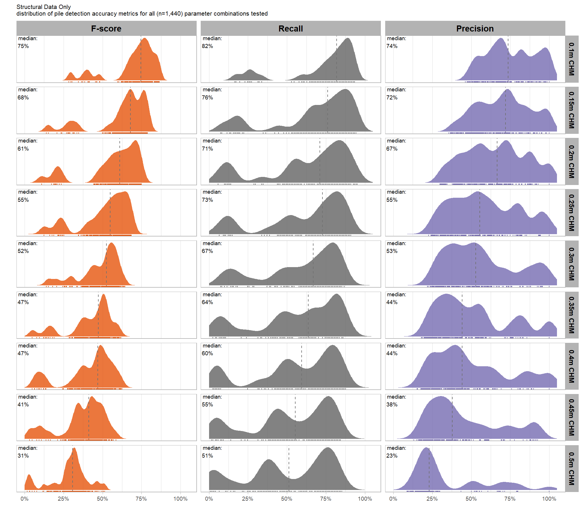
what is the detection accuracy across all parameter combinations tested for each CHM resolution?
# this is a lot of work, so we're going to make it a function
plt_detection_dist2 <- function(
  df
  , my_subtitle = ""
  , show_rug = T
) {
  # Construct the formula for facet_grid
  # facet_formula <- reformulate("metric", "chm_res_m_desc") # reformulate(col_facet_var, row_facet_var)

  pal_eval_metric <- c(
    RColorBrewer::brewer.pal(3,"Oranges")[3]
    , RColorBrewer::brewer.pal(3,"Greys")[3]
    , RColorBrewer::brewer.pal(3,"Purples")[3]
  )

  df_temp <- df %>%
    tidyr::pivot_longer(
      cols = c(precision,recall,f_score)
      , names_to = "metric"
      , values_to = "value"
    ) %>%
    dplyr::mutate(
      metric = dplyr::case_when(
          metric == "f_score" ~ 1
          , metric == "recall" ~ 2
          , metric == "precision" ~ 3
        ) %>%
        factor(
          ordered = T
          , levels = 1:3
          , labels = c(
            "F-score"
            , "Recall"
            , "Precision"
          )
        )
    )

  # chm check
  nrow_check <- df %>%
    dplyr::count(chm_res_m_desc) %>%
    dplyr::pull(n) %>%
    max()

  # plot
  if(nrow_check<=15){
    # round
    df_temp <- df_temp %>%
      dplyr::mutate(
        value = round(value,2)
      )
    # agg for median plotting
    xxxdf_temp <- df_temp %>%
      dplyr::group_by(chm_res_m_desc,metric) %>%
      dplyr::summarise(value = median(value,na.rm=T)) %>%
      dplyr::ungroup() %>%
      dplyr::mutate(
        value_lab = paste0(
          "median:\n"
          , scales::percent(value,accuracy=1)
        )
      )

    # plot
    plt <- df_temp %>%
      dplyr::count(chm_res_m_desc,metric,value) %>%
      ggplot2::ggplot(
        mapping = ggplot2::aes(x = value, fill = metric, color = metric)
      ) +
      ggplot2::geom_vline(
        data = xxxdf_temp
        , mapping = ggplot2::aes(xintercept = value)
        , color = "gray44", linetype = "dashed"
      ) +
      # ggplot2::geom_jitter(mapping = ggplot2::aes(y=-0.2), width = 0, height = 0.1) +
      # ggplot2::geom_boxplot(width = 0.1, color = "black", fill = NA, outliers = F) +
      ggplot2::geom_segment(
        mapping = ggplot2::aes(y=n,yend=0)
        , lwd = 2, alpha = 0.8
      ) +
      ggplot2::geom_point(
        mapping = ggplot2::aes(y=n)
        , alpha = 1
        , shape = 21, color = "gray44", size = 5
      ) +
      ggplot2::geom_text(
        mapping = ggplot2::aes(y=n,label=n)
        , size = 2.5, color = "white"
        # , vjust = -0.01
      ) +
      ggplot2::geom_text(
        data = xxxdf_temp
        , mapping = ggplot2::aes(
          x = -Inf, y = Inf # always in upper left?
          # x = value, y = 0
          , label = value_lab
        )
        , hjust = -0.1, vjust = 1 # always in upper left?
        # , hjust = -0.1, vjust = -5
        , size = 2.5, color = "black"
      ) +
      # ggplot2::geom_rug() +
      ggplot2::scale_fill_manual(values = pal_eval_metric) +
      ggplot2::scale_color_manual(values = pal_eval_metric) +
      ggplot2::scale_y_continuous(expand = ggplot2::expansion(mult = c(0, .2))) +
      ggplot2::scale_x_continuous(
        labels = scales::percent_format(accuracy = 1)
        # , limits = c(0,1.05)
      ) +
      ggplot2::facet_grid(cols = dplyr::vars(metric), rows = dplyr::vars(chm_res_m_desc), scales = "free_x") +
      ggplot2::labs(
        x = "", y = ""
        , subtitle = my_subtitle
      ) +
      ggplot2::theme_light() +
      ggplot2::theme(
        legend.position = "none"
        , strip.text = ggplot2::element_text(size = 11, color = "black", face = "bold")
        , axis.text.x = ggplot2::element_text(size = 7)
        , axis.text.y = ggplot2::element_blank()
        , axis.ticks.y = ggplot2::element_blank()
        , panel.grid.major.y = ggplot2::element_blank()
        , panel.grid.minor.y = ggplot2::element_blank()
        , plot.subtitle = ggplot2::element_text(size = 8)
      )
  }else{
    # agg for median plotting
    xxxdf_temp <- df_temp %>%
      dplyr::group_by(chm_res_m_desc,metric) %>%
      dplyr::summarise(value = median(value,na.rm=T)) %>%
      dplyr::ungroup() %>%
      dplyr::mutate(
        value_lab = paste0(
          "median:\n"
          , scales::percent(value,accuracy=1)
        )
      )
    plt <- df_temp %>%
      ggplot2::ggplot(
        mapping = ggplot2::aes(x = value, fill = metric, color = metric)
      ) +
      ggplot2::geom_density(mapping = ggplot2::aes(y=ggplot2::after_stat(scaled)), color = NA, alpha = 0.8) +
      # ggplot2::geom_rug(
      #   # # setting these makes the plotting more computationally intensive
      #   # alpha = 0.5
      #   # , length = ggplot2::unit(0.01, "npc")
      # ) +
      ggplot2::geom_vline(
        data = xxxdf_temp
        , mapping = ggplot2::aes(xintercept = value)
        , color = "gray44", linetype = "dashed"
      ) +
      ggplot2::geom_text(
        data = xxxdf_temp
        , mapping = ggplot2::aes(
          x = -Inf, y = Inf # always in upper left?
          # x = value, y = 0
          , label = value_lab
        )
        , hjust = -0.1, vjust = 1 # always in upper left?
        # , hjust = -0.1, vjust = -5
        , size = 2.5, color = "black"
      ) +
      ggplot2::scale_fill_manual(values = pal_eval_metric) +
      ggplot2::scale_color_manual(values = pal_eval_metric) +
      ggplot2::scale_x_continuous(
        labels = scales::percent_format(accuracy = 1)
        , limits = c(0,1.05)
      ) +
      ggplot2::facet_grid(cols = dplyr::vars(metric), rows = dplyr::vars(chm_res_m_desc), scales = "free_y") +
      ggplot2::labs(
        x = "", y = ""
        , subtitle = my_subtitle
      ) +
      ggplot2::theme_light() +
      ggplot2::theme(
        legend.position = "none"
        , strip.text.x = ggplot2::element_text(size = 11, color = "black", face = "bold")
        , strip.text.y = ggplot2::element_text(size = 9, color = "black", face = "bold")
        , axis.text.x = ggplot2::element_text(size = 7)
        , axis.text.y = ggplot2::element_blank()
        , axis.ticks.y = ggplot2::element_blank()
        , panel.grid.major.y = ggplot2::element_blank()
        , panel.grid.minor.y = ggplot2::element_blank()
        , plot.subtitle = ggplot2::element_text(size = 8)
      )
    if(show_rug){
      plt <- plt +
        ggplot2::geom_rug(
          # # setting these makes the plotting more computationally intensive
          # alpha = 0.5
          # , length = ggplot2::unit(0.01, "npc")
        )
    }
  }
  return(plt)
}
# plot it
plt_detection_dist2(
df = param_combos_gt_agg
, paste0(
"Structural Data Only"
, "\ndistribution of pile detection accuracy metrics for all"
, " (n="
, scales::comma(n_combos_tested_chm, accuracy = 1)
, ") "
, "parameter combinations tested"
)
)
collapsing across all other parameters, what is the main effect of each individual parameter or CHM resolution?
param_combos_gt_agg %>%
  tidyr::pivot_longer(
    cols = c(precision,recall,f_score)
    , names_to = "metric"
    , values_to = "value"
  ) %>%
  tidyr::pivot_longer(
    cols = c(max_ht_m,max_area_m2,convexity_pct,circle_fit_iou_pct,chm_res_m)
    , names_to = "param"
    , values_to = "param_value"
  ) %>%
  dplyr::group_by(param, param_value, metric) %>%
  dplyr::summarise(
    median = median(value,na.rm=T)
    , q25 = stats::quantile(value,na.rm=T,probs = 0.25)
    , q75 = stats::quantile(value,na.rm=T,probs = 0.75)
  ) %>%
  dplyr::ungroup() %>%
  dplyr::mutate(
    param = dplyr::case_when(
        param == "chm_res_m" ~ 1
        , param == "max_ht_m" ~ 2
        , param == "min_area_m2" ~ 3
        , param == "max_area_m2" ~ 4
        , param == "convexity_pct" ~ 5
        , param == "circle_fit_iou_pct" ~ 6
      ) %>%
      factor(
        ordered = T
        , levels = 1:6
        , labels = c(
          "CHM resolution (m)"
          , "max_ht_m"
          , "min_area_m2"
          , "max_area_m2"
          , "convexity_pct"
          , "circle_fit_iou_pct"
        )
      )
    , metric = dplyr::case_when(
        metric == "f_score" ~ 1
        , metric == "recall" ~ 2
        , metric == "precision" ~ 3
      ) %>%
      factor(
        ordered = T
        , levels = 1:3
        , labels = c(
          "F-score"
          , "Recall"
          , "Precision"
        )
      ) %>%
      forcats::fct_rev()
  ) %>%
  ggplot2::ggplot(
    mapping = ggplot2::aes(y = median, x = param_value, color = metric, fill = metric, group = metric, shape = metric)
  ) +
  ggplot2::geom_ribbon(
    mapping = ggplot2::aes(ymin = q25, ymax = q75)
    , alpha = 0.2, color = NA
  ) +
  ggplot2::geom_line(lwd = 1.5, alpha = 0.8) +
  ggplot2::geom_point(size = 2) +
  ggplot2::facet_wrap(facets = dplyr::vars(param), scales = "free_x") +
  # ggplot2::scale_color_viridis_d(begin = 0.2, end = 0.8) +
  ggplot2::scale_fill_manual(values = rev(pal_eval_metric)) +
  ggplot2::scale_color_manual(values = rev(pal_eval_metric)) +
  ggplot2::scale_y_continuous(limits = c(0,1), labels = scales::percent, breaks = scales::breaks_extended(10)) +
  ggplot2::labs(
    x = "", y = "median value", color = "", fill = ""
    , subtitle = "Structural Data Only"
  ) +
  ggplot2::theme_light() +
  ggplot2::theme(
    legend.position = "top"
    , strip.text = ggplot2::element_text(size = 11, color = "black", face = "bold")
  ) +
  ggplot2::guides(
    color = ggplot2::guide_legend(override.aes = list(shape = 15, linetype = 0, size = 5, alpha = 1))
    , shape = "none"
  )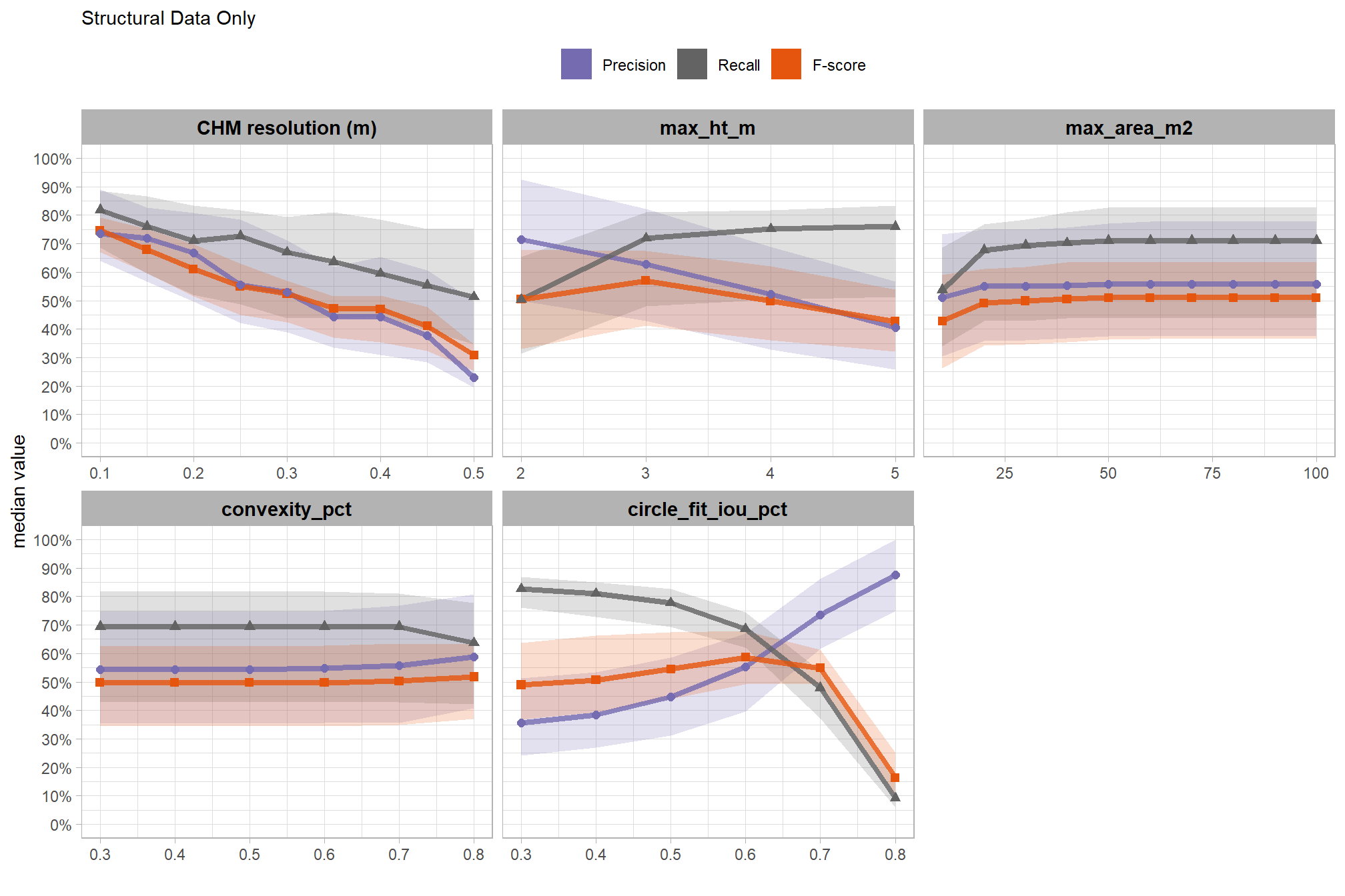
based on these main effect aggregated results using our point cloud and validation data:
- increasing the CHM resolution (making it more coarse) consistently reduced all detection accuracy metrics (F-score, precision, and recall) across the tested range of 0.1m to 0.5m
- increasing the
max_ht_m(which sets the maximum height of the CHM slice) steadily reduced precision. conversely, F-score and recall improved when the parameter was increased from 2 m to 3 m, remaining stable or slightly declining thereafter - increasing the
max_area_m2(which determines the maximum pile area) had minimal impact on detection metrics once the value was set above 10 m2. however, an increase from 10 m2 to 20 m2 improved all three detection accuracy metrics given the data used in this study - increasing
convexity_pct(toward 1 to favor more regular shapes) had minimal impact on metrics until values exceeded 0.7. at this point, recall decreased, but precision and F-score saw slight improvements - increasing
circle_fit_iou_pct(toward 1 to favor circular shapes) improved precision and F-score up to a value of 0.5 with minimal effect on recall. Beyond this point, recall dropped significantly, with only modest improvements to F-score, and overall accuracy crashed past 0.7.
9.5.2 Main Effects: form quantification
let’s check out the the ability of the method to properly extract the form of the piles by looking at the quantification accuracy metrics where:
- Mean Error (ME) represents the direction of bias (over or under-prediction) in the original units
- RMSE represents the typical magnitude of error in the original units, with a stronger penalty for large errors
- MAPE represents the typical magnitude of error as a percentage, allowing for scale-independent comparisons
as a reminder regarding the form quantification accuracy evaluation, we will assess the method’s accuracy by comparing the true-positive matches using the following metrics:
- Volume compares the predicted volume from the irregular elevation profile and footprint to the ground truth paraboloid volume
- Diameter compares the predicted diameter (from the maximum internal distance) to the ground truth field-measured diameter.
- Area compares the predicted area from the irregular shape to the ground truth assumed circular area
- Height compares the predicted maximum height from the CHM to the ground truth field-measured height
what is the quantification accuracy across all parameter combinations tested for each CHM resolution?
# let's average across all other factors to look at the main effect by parameter for the **MAPE** metrics quantifying the pile form accuracy
# this is a lot of work, so we're going to make it a function
plt_form_quantification_trend <- function(
df
, my_subtitle = ""
, quant_metric = "mape" # rmse, mean, mape
) {
quant_metric <- dplyr::case_when(
tolower(quant_metric) == "mape" ~ "mape"
, tolower(quant_metric) == "rmse" ~ "rmse"
, tolower(quant_metric) == "mean" ~ "mean"
, T ~ "mape"
)
p <- df %>%
tidyr::pivot_longer(
cols = tidyselect::ends_with(paste0("_",quant_metric))
, names_to = "metric"
, values_to = "value"
) %>%
tidyr::pivot_longer(
cols = c(max_ht_m,max_area_m2,convexity_pct,circle_fit_iou_pct,chm_res_m)
, names_to = "param"
, values_to = "param_value"
) %>%
dplyr::group_by(param, param_value, metric) %>%
dplyr::summarise(
median = median(value,na.rm=T)
, q25 = stats::quantile(value,na.rm=T,probs = 0.25)
, q75 = stats::quantile(value,na.rm=T,probs = 0.75)
) %>%
dplyr::ungroup() %>%
dplyr::mutate(
param = dplyr::case_when(
param == "chm_res_m" ~ 1
, param == "max_ht_m" ~ 2
, param == "min_area_m2" ~ 3
, param == "max_area_m2" ~ 4
, param == "convexity_pct" ~ 5
, param == "circle_fit_iou_pct" ~ 6
) %>%
factor(
ordered = T
, levels = 1:6
, labels = c(
"CHM resolution (m)"
, "max_ht_m"
, "min_area_m2"
, "max_area_m2"
, "convexity_pct"
, "circle_fit_iou_pct"
)
)
, pile_metric = metric %>%
stringr::str_remove("(_rmse|_rrmse|_mean|_mape)$") %>%
stringr::str_extract("(paraboloid_volume|volume|area|height|diameter)") %>%
factor(
ordered = T
, levels = c(
"volume"
, "paraboloid_volume"
, "area"
, "height"
, "diameter"
)
, labels = c(
"Volume"
, "Volume paraboloid"
, "Area"
, "Height"
, "Diameter"
)
)
) %>%
ggplot2::ggplot(
mapping = ggplot2::aes(y = median, x = param_value, color = pile_metric, fill = pile_metric, group = pile_metric) #, shape = pile_metric)
) +
# ggplot2::geom_ribbon(
# mapping = ggplot2::aes(ymin = q25, ymax = q75)
# , alpha = 0.2, color = NA
# ) +
ggplot2::geom_line(lwd = 1.5, alpha = 0.8) +
ggplot2::geom_point(size = 2) +
ggplot2::facet_grid(cols = dplyr::vars(param), rows = dplyr::vars(pile_metric), scales = "free", axes = "all") +
# ggplot2::scale_color_viridis_d(begin = 0.2, end = 0.8) +
ggplot2::scale_fill_viridis_d(option = "turbo") +
ggplot2::scale_color_viridis_d(option = "turbo") +
ggplot2::labs(
x = ""
, y = paste0(ifelse(quant_metric=="mean","Mean Error", toupper(quant_metric)), " (median)")
, color = "", fill = ""
, title = ifelse(quant_metric=="mean","Mean Error", toupper(quant_metric))
) +
ggplot2::theme_light() +
ggplot2::theme(
legend.position = "none"
, strip.text = ggplot2::element_text(size = 11, color = "black", face = "bold")
, axis.text.x = ggplot2::element_text(size = 7)
, axis.text.y = ggplot2::element_text(size = 8)
) +
ggplot2::guides(
color = ggplot2::guide_legend(override.aes = list(shape = 15, linetype = 0, size = 5, alpha = 1))
, shape = "none"
)
if(quant_metric == "mape"){
p <- p +
ggplot2::scale_y_continuous(labels = scales::percent, breaks = scales::breaks_extended(10))
}else{
p <- p +
ggplot2::scale_y_continuous(labels = scales::comma, breaks = scales::breaks_extended(10))
}
return(p)
}
# plt_form_quantification_trend(param_combos_gt_agg, quant_metric = "mean")
# plt_form_quantification_trend(param_combos_gt_agg, quant_metric = "mape")
# this is a lot of work, so we're going to make it a function
plt_form_quantification_dist2 <- function(
df
, my_subtitle = ""
, show_rug = T
, quant_metric = "mape" # rmse, mean, mape
) {
# reshape data to go long by evaluation metric
df_temp <-
df %>%
dplyr::ungroup() %>%
dplyr::select(
max_ht_m,max_area_m2,convexity_pct,circle_fit_iou_pct,chm_res_m_desc,chm_res_m
# quantification
, tidyselect::ends_with("_rmse")
, tidyselect::ends_with("_rrmse")
, tidyselect::ends_with("_mean")
, tidyselect::ends_with("_mape")
) %>%
tidyr::pivot_longer(
cols = c(
tidyselect::ends_with("_rmse")
, tidyselect::ends_with("_rrmse")
, tidyselect::ends_with("_mean")
, tidyselect::ends_with("_mape")
)
, names_to = "metric"
, values_to = "value"
) %>%
dplyr::mutate(
eval_metric = stringr::str_extract(metric, "(_rmse|_rrmse|_mean|_mape)$") %>%
stringr::str_remove_all("_") %>%
stringr::str_replace_all("mean","me") %>%
toupper() %>%
factor(
ordered = T
, levels = c("ME","RMSE","RRMSE","MAPE")
)
, pile_metric = metric %>%
stringr::str_remove("(_rmse|_rrmse|_mean|_mape)$") %>%
stringr::str_extract("(paraboloid_volume|volume|area|height|diameter)") %>%
factor(
ordered = T
, levels = c(
"volume"
, "paraboloid_volume"
, "area"
, "height"
, "diameter"
)
, labels = c(
"Volume"
, "Volume paraboloid"
, "Area"
, "Height"
, "Diameter"
)
)
)
# plot
# chm check
nrow_check <- df %>%
dplyr::count(chm_res_m_desc) %>%
dplyr::pull(n) %>%
max()
# plot
if(nrow_check<=15){
# round
df_temp <- df_temp %>%
dplyr::filter(
eval_metric==dplyr::case_when(
tolower(quant_metric) == "mape" ~ "MAPE"
, tolower(quant_metric) == "rmse" ~ "RMSE"
, tolower(quant_metric) == "mean" ~ "ME"
, T ~ "MAPE"
)
) %>%
dplyr::mutate(
value = dplyr::case_when(
eval_metric %in% c("RRMSE", "MAPE") ~ round(value,2)
, T ~ round(value,1)
)
)
# agg for median plotting
xxxdf_temp <- df_temp %>%
dplyr::group_by(chm_res_m_desc,pile_metric,eval_metric) %>%
dplyr::summarise(value = median(value,na.rm=T)) %>%
dplyr::ungroup() %>%
dplyr::mutate(
value_lab = paste0(
"median:\n"
, dplyr::case_when(
eval_metric %in% c("RRMSE", "MAPE") ~ scales::percent(value,accuracy=1)
, eval_metric == "ME" ~ scales::comma(value,accuracy=0.1)
, T ~ scales::comma(value,accuracy=0.1)
)
)
)
# plot
p <-
df_temp %>%
dplyr::count(chm_res_m_desc,pile_metric,value) %>%
ggplot2::ggplot(mapping = ggplot2::aes(x=value,color = pile_metric,fill = pile_metric)) +
ggplot2::geom_vline(
data = xxxdf_temp %>%
dplyr::filter(
eval_metric==dplyr::case_when(
tolower(quant_metric) == "mape" ~ "MAPE"
, tolower(quant_metric) == "rmse" ~ "RMSE"
, tolower(quant_metric) == "mean" ~ "ME"
, T ~ "MAPE"
)
)
, mapping = ggplot2::aes(xintercept = value)
, color = "gray44", linetype = "dashed"
) +
ggplot2::geom_segment(
mapping = ggplot2::aes(y=n,yend=0)
, lwd = 2, alpha = 0.8
) +
ggplot2::geom_point(
mapping = ggplot2::aes(y=n)
, alpha = 1
, shape = 21, color = "gray44", size = 5
) +
ggplot2::geom_text(
mapping = ggplot2::aes(y=n,label=n)
, size = 2.5, color = "white"
# , vjust = -0.01
) +
ggplot2::scale_y_continuous(expand = ggplot2::expansion(mult = c(0, .2))) +
ggplot2::scale_fill_viridis_d(option = "turbo") +
ggplot2::scale_color_viridis_d(option = "turbo") +
ggplot2::geom_text(
data = xxxdf_temp %>%
dplyr::filter(
eval_metric==dplyr::case_when(
tolower(quant_metric) == "mape" ~ "MAPE"
, tolower(quant_metric) == "rmse" ~ "RMSE"
, tolower(quant_metric) == "mean" ~ "ME"
, T ~ "MAPE"
)
)
, mapping = ggplot2::aes(
x = -Inf, y = Inf # always in upper left?
# x = value, y = 0
, label = value_lab
)
, hjust = -0.1, vjust = 1 # always in upper left?
# , hjust = -0.1, vjust = -5
, size = 2.5
, color = "black"
) +
ggplot2::facet_grid(cols = dplyr::vars(pile_metric), rows = dplyr::vars(chm_res_m_desc), scales = "free") +
ggplot2::labs(
x = "", y = ""
, subtitle = my_subtitle
, title = dplyr::case_when(
tolower(quant_metric) == "mape" ~ "MAPE"
, tolower(quant_metric) == "rmse" ~ "RMSE"
, tolower(quant_metric) == "mean" ~ "Mean Error"
, T ~ "MAPE"
)
) +
ggplot2::theme_light() +
ggplot2::theme(
legend.position = "none"
, strip.text.x = ggplot2::element_text(size = 11, color = "black", face = "bold")
, strip.text.y = ggplot2::element_text(size = 9, color = "black", face = "bold")
, axis.text.x = ggplot2::element_text(size = 7)
, axis.text.y = ggplot2::element_blank()
, axis.ticks.y = ggplot2::element_blank()
, panel.grid.major.y = ggplot2::element_blank()
, panel.grid.minor.y = ggplot2::element_blank()
, plot.subtitle = ggplot2::element_text(size = 8)
)
}else{
# aggregate
xxxdf_temp <- df_temp %>%
dplyr::group_by(chm_res_m_desc,pile_metric,eval_metric) %>%
dplyr::summarise(value = median(value,na.rm=T)) %>%
dplyr::ungroup() %>%
dplyr::mutate(
value_lab = paste0(
"median:\n"
, dplyr::case_when(
eval_metric %in% c("RRMSE", "MAPE") ~ scales::percent(value,accuracy=0.1)
, eval_metric == "ME" ~ scales::comma(value,accuracy=0.01)
, T ~ scales::comma(value,accuracy=0.1)
)
)
)
p <-
df_temp %>%
dplyr::filter(
eval_metric==dplyr::case_when(
tolower(quant_metric) == "mape" ~ "MAPE"
, tolower(quant_metric) == "rmse" ~ "RMSE"
, tolower(quant_metric) == "mean" ~ "ME"
, T ~ "MAPE"
)
) %>%
ggplot2::ggplot() +
# ggplot2::geom_vline(xintercept = 0, color = "gray") +
ggplot2::geom_density(mapping = ggplot2::aes(x = value, y = ggplot2::after_stat(scaled), fill = pile_metric), color = NA, alpha = 0.8) +
ggplot2::scale_fill_viridis_d(option = "turbo") +
ggplot2::scale_color_viridis_d(option = "turbo") +
ggplot2::geom_vline(
data = xxxdf_temp %>%
dplyr::filter(
eval_metric==dplyr::case_when(
tolower(quant_metric) == "mape" ~ "MAPE"
, tolower(quant_metric) == "rmse" ~ "RMSE"
, tolower(quant_metric) == "mean" ~ "ME"
, T ~ "MAPE"
)
)
, mapping = ggplot2::aes(xintercept = value)
, color = "gray44", linetype = "dashed"
) +
ggplot2::geom_text(
data = xxxdf_temp %>%
dplyr::filter(
eval_metric==dplyr::case_when(
tolower(quant_metric) == "mape" ~ "MAPE"
, tolower(quant_metric) == "rmse" ~ "RMSE"
, tolower(quant_metric) == "mean" ~ "ME"
, T ~ "MAPE"
)
)
, mapping = ggplot2::aes(
x = -Inf, y = Inf # always in upper left?
# x = value, y = 0
, label = value_lab
)
, hjust = -0.1, vjust = 1 # always in upper left?
# , hjust = -0.1, vjust = -5
, size = 2.5
) +
ggplot2::facet_grid(cols = dplyr::vars(pile_metric), rows = dplyr::vars(chm_res_m_desc), scales = "free") +
ggplot2::labs(
x = "", y = ""
, subtitle = my_subtitle
, title = dplyr::case_when(
tolower(quant_metric) == "mape" ~ "MAPE"
, tolower(quant_metric) == "rmse" ~ "RMSE"
, tolower(quant_metric) == "mean" ~ "Mean Error"
, T ~ "MAPE"
)
) +
ggplot2::theme_light() +
ggplot2::theme(
legend.position = "none"
, strip.text.x = ggplot2::element_text(size = 11, color = "black", face = "bold")
, strip.text.y = ggplot2::element_text(size = 9, color = "black", face = "bold")
, axis.text.x = ggplot2::element_text(size = 7)
, axis.text.y = ggplot2::element_blank()
, axis.ticks.y = ggplot2::element_blank()
, panel.grid.major.y = ggplot2::element_blank()
, panel.grid.minor.y = ggplot2::element_blank()
, plot.subtitle = ggplot2::element_text(size = 8)
)
if(show_rug){
p <- p + ggplot2::geom_rug(mapping = ggplot2::aes(x = value, color = pile_metric))
}
}
if(
dplyr::case_when(
tolower(quant_metric) == "mape" ~ "MAPE"
, tolower(quant_metric) == "rmse" ~ "RMSE"
, tolower(quant_metric) == "mean" ~ "ME"
, T ~ "MAPE"
) %in% c("RRMSE", "MAPE")
){
return(p+ggplot2::scale_x_continuous(labels = scales::percent_format(accuracy = 1)))
}else{
return(p)
}
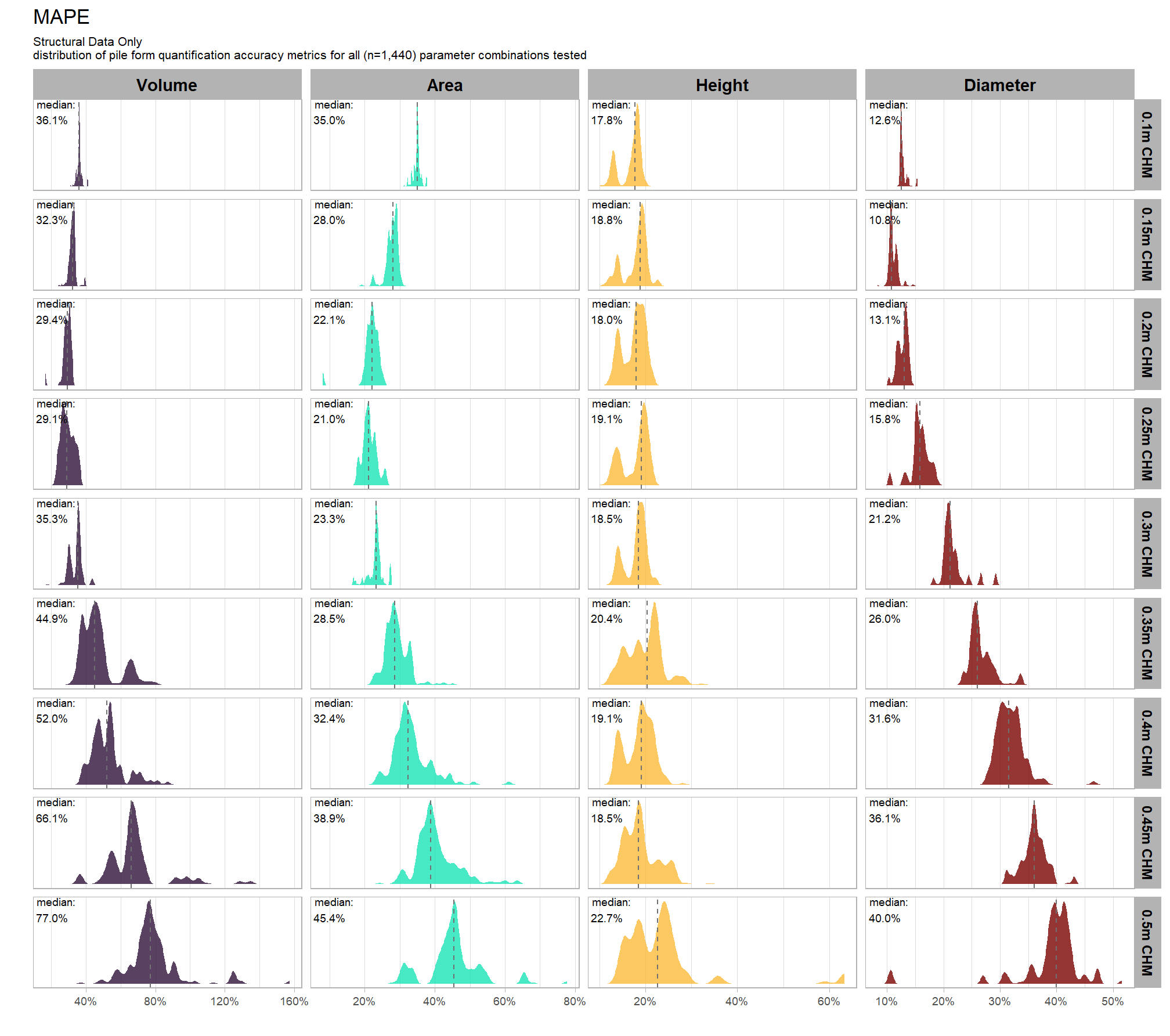
}9.5.2.1 MAPE
MAPE represents the typical magnitude of error as a percentage, allowing for scale-independent comparisons
distribution across all parameter combinations tested
# plot it
plt_form_quantification_dist2(
  df = param_combos_gt_agg
  , quant_metric = "mape"
  , paste0(
     "Structural Data Only"
      , "\ndistribution of pile form quantification accuracy metrics for all"
     , " (n="
     , scales::comma(n_combos_tested_chm, accuracy = 1)
     , ") "
     , "parameter combinations tested"
  )
  , show_rug = F
)
let’s average across all other factors to look at the median main effect by parameter and quantification metric
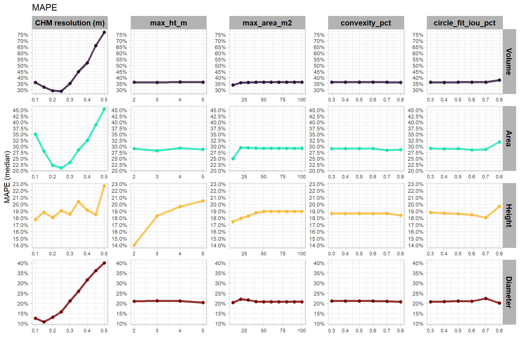
WHAT DID WE LEARN FROM THIS
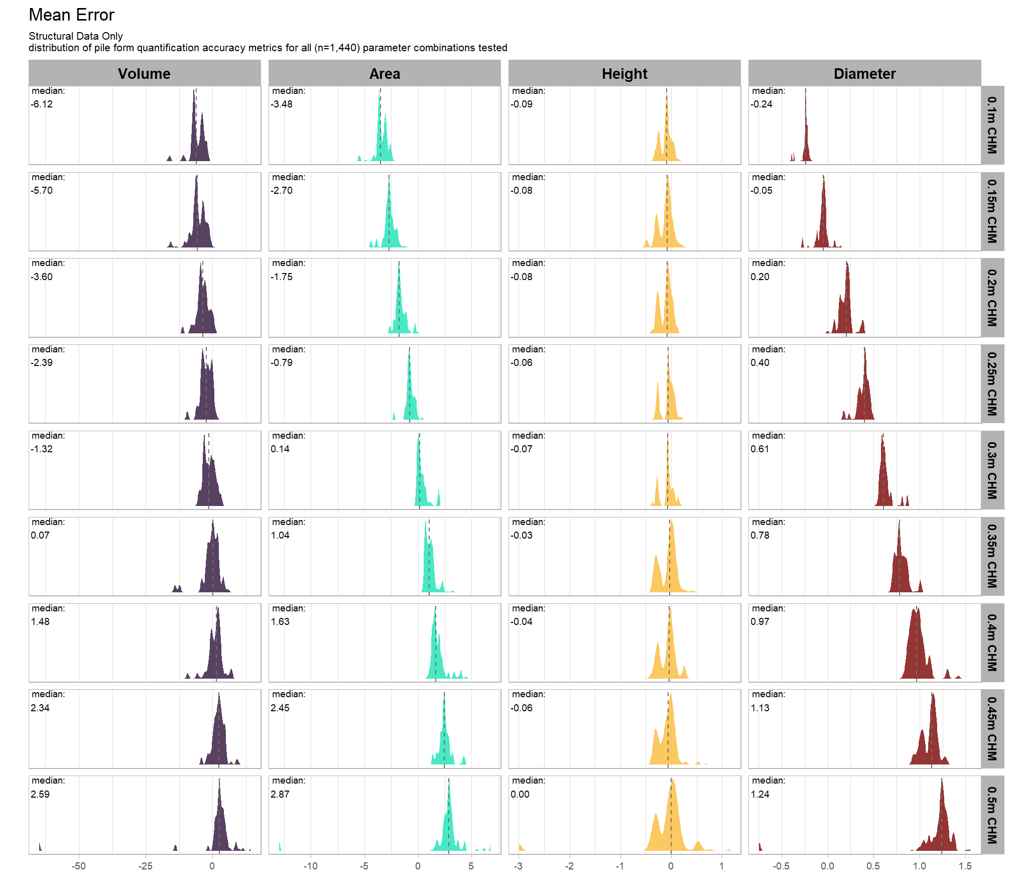
9.5.2.2 Mean Error (ME)
Mean Error (ME) represents the direction of bias (over or under-prediction) in the original units
distribution across all parameter combinations tested
# plot it
plt_form_quantification_dist2(
  df = param_combos_gt_agg
  , quant_metric = "mean"
  , paste0(
     "Structural Data Only"
      , "\ndistribution of pile form quantification accuracy metrics for all"
     , " (n="
     , scales::comma(n_combos_tested_chm, accuracy = 1)
     , ") "
     , "parameter combinations tested"
  )
  , show_rug = F
)
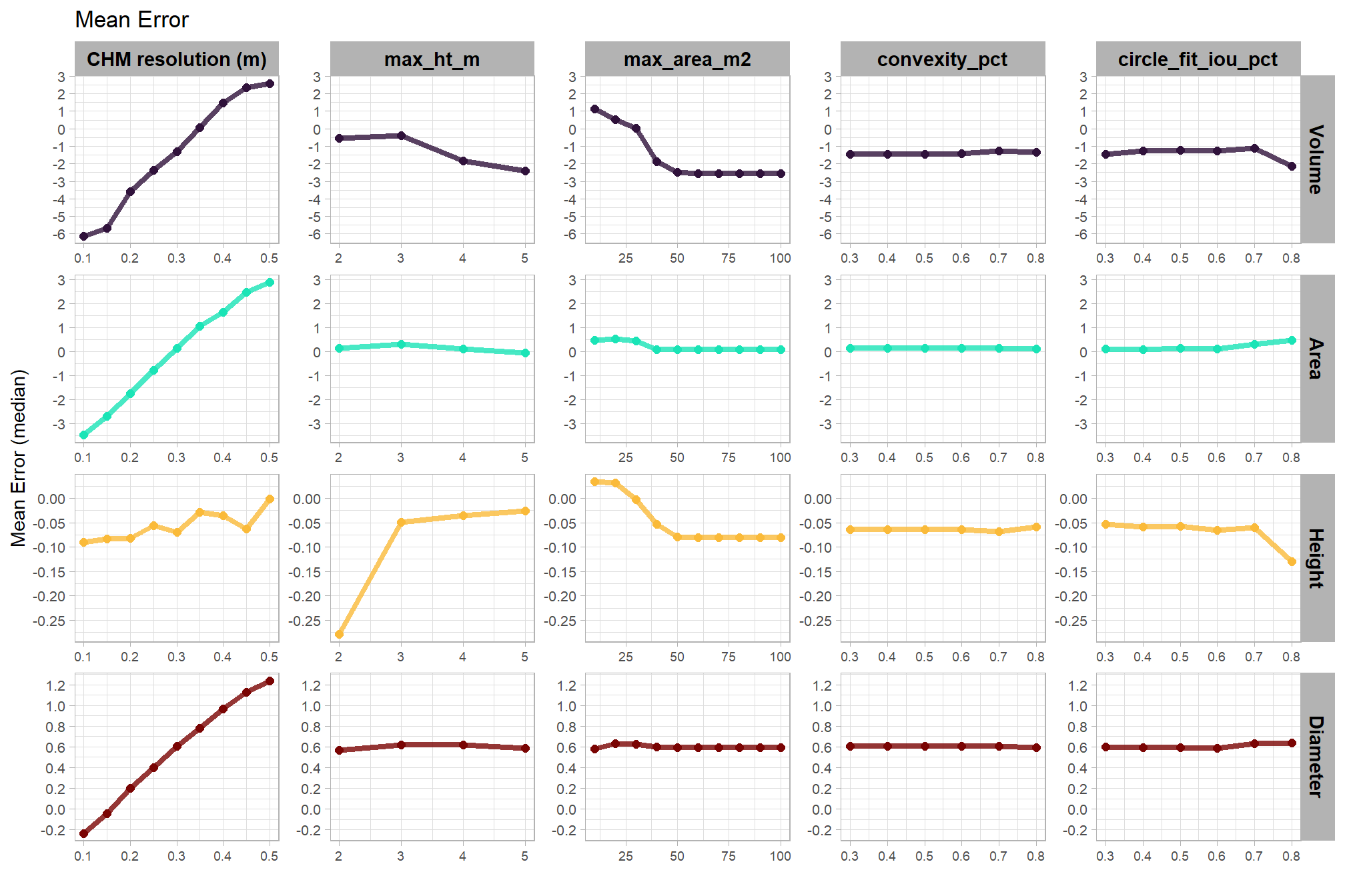
let’s average across all other factors to look at the median main effect by parameter and quantification metric
WHAT DID WE LEARN FROM THIS
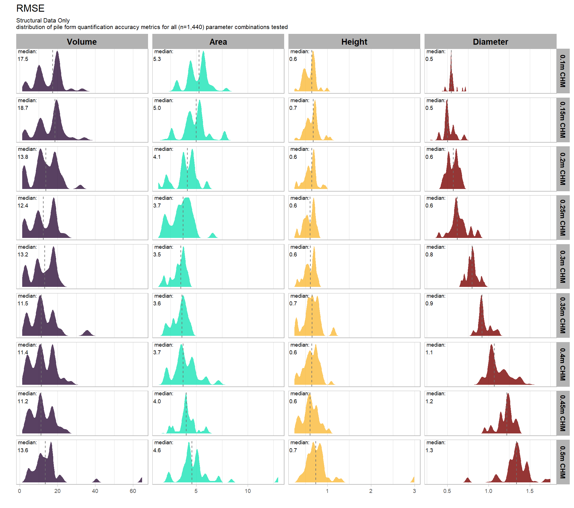
9.5.2.3 RMSE
RMSE represents the typical magnitude of error in the original units, with a stronger penalty for large errors
# plot it
plt_form_quantification_dist2(
  df = param_combos_gt_agg
  , quant_metric = "rmse"
  , paste0(
     "Structural Data Only"
      , "\ndistribution of pile form quantification accuracy metrics for all"
     , " (n="
     , scales::comma(n_combos_tested_chm, accuracy = 1)
     , ") "
     , "parameter combinations tested"
  )
  , show_rug = F
)
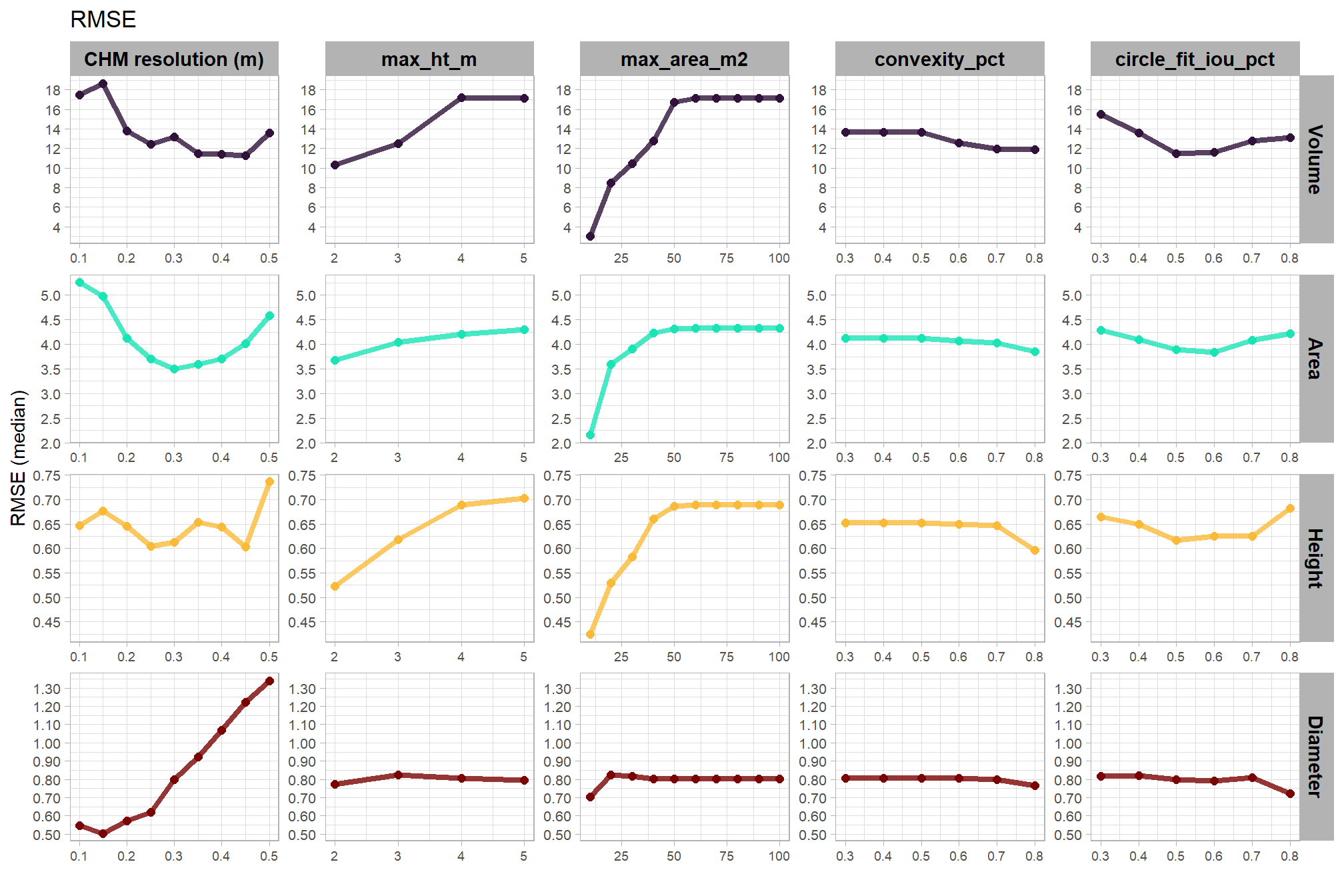
let’s average across all other factors to look at the median main effect by parameter and quantification metric
WHAT DID WE LEARN FROM THIS
9.5.3 Final recommended settings
let’s identify the best-performing parameter combinations that not only balance detection and quantification accuracy but also achieve the highest recall rates. we’ll select these by choosing any combination whose recall rate is at least one standard deviation above the average for this top group. if no combinations meet this criterion, we will instead select the top 10 combinations based on their recall rates.
9.5.3.1 Overall (across CHM resolution)
To select the best-performing parameter combinations, we will prioritize those that balance detection and quantification accuracy. From this group, we will then identify the settings that achieve the highest pile detection rates (recall). We emphasize that these recommendations are for users who can generate a CHM from the original point cloud. This is critical because creating a new CHM at the desired resolution is a fundamentally different process than simply disaggregating an existing, coarser raster.
we’ll use the F-Score and the average rank of the MAPE metrics across all form measurements (i.e. height, diameter, area, volume) to determine the best overall list
##################### START USER DEFINED #####################
# what percent should we classify as top?
pct_th_top <- 0.01
# of those top, how many should be selected by recall?
n_th_top <- 12
##################### END USER DEFINED #####################
# math on user defined to label stuff
# structural only
n_combos_top_overall <- n_combos_tested*pct_th_top
n_th_top_chm <- round(n_th_top/2)
pct_th_top_chm <- pct_th_top*2
n_combos_top_chm <- floor(n_combos_tested_chm*pct_th_top_chm) # double it so we look at more than 14??
n_combos_top_spectral_chm <- floor(n_combos_tested_spectral_chm*pct_th_top_chm)
# param_combos_gt_agg %>% nrow()
param_combos_ranked <-
param_combos_gt_agg %>%
##########
# first. find overall top combinations irrespective of CHM res
##########
dplyr::ungroup() %>%
dplyr::mutate(
# label combining params
lab = stringr::str_c(max_ht_m,max_area_m2,convexity_pct,circle_fit_iou_pct,chm_res_m, sep = ":")
, dplyr::across(
.cols = c(tidyselect::ends_with("_mape"))
, .fn = ~dplyr::percent_rank(-.x)
, .names = "ovrall_pct_rank_quant_{.col}"
)
, dplyr::across(
.cols = c(f_score)
# .cols = c(f_score,recall)
, .fn = ~dplyr::percent_rank(.x)
, .names = "ovrall_pct_rank_det_{.col}"
)
) %>%
##########
# second. find top combinations by CHM res
##########
dplyr::group_by(chm_res_m) %>%
dplyr::mutate(
dplyr::across(
.cols = c(tidyselect::ends_with("_mape") & !tidyselect::starts_with("ovrall_pct_rank_"))
, .fn = ~dplyr::percent_rank(-.x)
, .names = "chm_pct_rank_quant_{.col}"
)
, dplyr::across(
.cols = c(f_score)
# .cols = c(f_score,recall)
, .fn = ~dplyr::percent_rank(.x)
, .names = "chm_pct_rank_det_{.col}"
)
) %>%
# now get the max of these pct ranks by row
dplyr::rowwise() %>%
dplyr::mutate(
ovrall_pct_rank_quant_mean = mean(
dplyr::c_across(
tidyselect::starts_with("ovrall_pct_rank_quant_")
)
, na.rm = T
)
, ovrall_pct_rank_det_mean = mean(
dplyr::c_across(
tidyselect::starts_with("ovrall_pct_rank_det_")
)
, na.rm = T
)
, chm_pct_rank_quant_mean = mean(
dplyr::c_across(
tidyselect::starts_with("chm_pct_rank_quant_")
)
, na.rm = T
)
, chm_pct_rank_det_mean = mean(
dplyr::c_across(
tidyselect::starts_with("chm_pct_rank_det_")
)
, na.rm = T
)
) %>%
dplyr::ungroup() %>%
# now make quadrant var
dplyr::mutate(
# groupings for the quadrant plot
ovrall_accuracy_grp = dplyr::case_when(
ovrall_pct_rank_det_mean>=0.95 & ovrall_pct_rank_quant_mean>=0.95 ~ 1
, ovrall_pct_rank_det_mean>=0.90 & ovrall_pct_rank_quant_mean>=0.90 ~ 2
, ovrall_pct_rank_det_mean>=0.75 & ovrall_pct_rank_quant_mean>=0.75 ~ 3
, ovrall_pct_rank_det_mean>=0.50 & ovrall_pct_rank_quant_mean>=0.50 ~ 4
, ovrall_pct_rank_det_mean>=0.50 & ovrall_pct_rank_quant_mean<0.50 ~ 5
, ovrall_pct_rank_det_mean<0.50 & ovrall_pct_rank_quant_mean>=0.50 ~ 6
, T ~ 7
) %>%
factor(
ordered = T
, levels = 1:7
, labels = c(
"top 5% detection & quantification" # ovrall_pct_rank_mean>=0.95 & ovrall_pct_rank_f_score>=0.95 ~ 1
, "top 10% detection & quantification" # ovrall_pct_rank_mean>=0.90 & ovrall_pct_rank_f_score>=0.90 ~ 2
, "top 25% detection & quantification" # ovrall_pct_rank_mean>=0.75 & ovrall_pct_rank_f_score>=0.75 ~ 3
, "top 50% detection & quantification" # ovrall_pct_rank_mean>=0.50 & ovrall_pct_rank_f_score>=0.50 ~ 4
, "top 50% quantification" # ovrall_pct_rank_mean>=0.50 & ovrall_pct_rank_f_score<0.50 ~ 5
, "top 50% detection" # ovrall_pct_rank_mean<0.50 & ovrall_pct_rank_f_score>=0.50 ~ 6
, "bottom 50% detection & quantification"
)
)
, chm_accuracy_grp = dplyr::case_when(
chm_pct_rank_det_mean>=0.95 & chm_pct_rank_quant_mean>=0.95 ~ 1
, chm_pct_rank_det_mean>=0.90 & chm_pct_rank_quant_mean>=0.90 ~ 2
, chm_pct_rank_det_mean>=0.75 & chm_pct_rank_quant_mean>=0.75 ~ 3
, chm_pct_rank_det_mean>=0.50 & chm_pct_rank_quant_mean>=0.50 ~ 4
, chm_pct_rank_det_mean>=0.50 & chm_pct_rank_quant_mean<0.50 ~ 5
, chm_pct_rank_det_mean<0.50 & chm_pct_rank_quant_mean>=0.50 ~ 6
, T ~ 7
) %>%
factor(
ordered = T
, levels = 1:7
, labels = c(
"top 5% detection & quantification" # chm_pct_rank_mean>=0.95 & chm_pct_rank_f_score>=0.95 ~ 1
, "top 10% detection & quantification" # chm_pct_rank_mean>=0.90 & chm_pct_rank_f_score>=0.90 ~ 2
, "top 25% detection & quantification" # chm_pct_rank_mean>=0.75 & chm_pct_rank_f_score>=0.75 ~ 3
, "top 50% detection & quantification" # chm_pct_rank_mean>=0.50 & chm_pct_rank_f_score>=0.50 ~ 4
, "top 50% quantification" # chm_pct_rank_mean>=0.50 & chm_pct_rank_f_score<0.50 ~ 5
, "top 50% detection" # chm_pct_rank_mean<0.50 & chm_pct_rank_f_score>=0.50 ~ 6
, "bottom 50% detection & quantification"
)
)
,
) %>%
##########
# first. find overall top combinations irrespective of CHM res
##########
dplyr::ungroup() %>%
dplyr::mutate(
ovrall_balanced_pct_rank = dplyr::percent_rank( (ovrall_pct_rank_det_mean+ovrall_pct_rank_quant_mean)/2 ) # equally weight quant and detection
, ovrall_lab = forcats::fct_reorder(lab, ovrall_balanced_pct_rank)
) %>%
dplyr::arrange(desc(ovrall_balanced_pct_rank),desc(ovrall_pct_rank_det_mean),desc(ovrall_pct_rank_quant_mean)) %>%
dplyr::mutate(
ovrall_balanced_rank = dplyr::row_number()
# is_top_overall = using rows in case not all combos resulted in piles and/or
# there are many ties in the data leading to no records with a percent rank <= pct_th_top (e.g. many tied at 98%)
, is_top_overall = dplyr::row_number()<=(n_combos_top_overall)
# ovrall_balanced_pct_rank>=(1-pct_th_top)
) %>%
dplyr::arrange(desc(is_top_overall),desc(recall),desc(ovrall_pct_rank_det_mean),desc(ovrall_pct_rank_quant_mean),ovrall_balanced_rank) %>%
dplyr::mutate(is_final_selection = is_top_overall & dplyr::row_number()<=n_th_top) %>%
##########
# second. find top combinations by CHM res
##########
dplyr::group_by(chm_res_m) %>%
dplyr::mutate(
chm_balanced_pct_rank = dplyr::percent_rank( (chm_pct_rank_det_mean+chm_pct_rank_quant_mean)/2 ) # equally weight quant and detection
, chm_lab = forcats::fct_reorder(lab, chm_balanced_pct_rank)
) %>%
dplyr::arrange(chm_res_m,desc(chm_balanced_pct_rank),desc(chm_pct_rank_det_mean),desc(chm_pct_rank_quant_mean),ovrall_balanced_rank) %>%
dplyr::mutate(
chm_balanced_rank = dplyr::row_number()
# is_top_chm = using rows in case not all combos resulted in piles and/or
# there are many ties in the data leading to no records with a percent rank <= pct_th_top (e.g. many tied at 98%)
, is_top_chm = dplyr::row_number()<=n_combos_top_chm # double it so we look at more than 14??
# chm_balanced_pct_rank>=(1-pct_th_top)
) %>%
dplyr::arrange(chm_res_m,desc(is_top_chm),desc(recall),desc(chm_pct_rank_det_mean),desc(chm_pct_rank_quant_mean),ovrall_balanced_rank) %>%
dplyr::mutate(is_final_selection_chm = is_top_chm & dplyr::row_number()<=n_th_top_chm) %>% # half it because it's going to be a lot to show in our facet ggplot
##### clean up
dplyr::ungroup() %>%
dplyr::select(-c(
c(tidyselect::ends_with("_mape") & tidyselect::starts_with("ovrall_pct_rank_"))
, c(tidyselect::ends_with("_mape") & tidyselect::starts_with("chm_pct_rank_"))
, c(tidyselect::ends_with("_f_score") & tidyselect::starts_with("ovrall_pct_rank_"))
, c(tidyselect::ends_with("_f_score") & tidyselect::starts_with("chm_pct_rank_"))
))
# huh?
# param_combos_ranked %>% dplyr::glimpse()
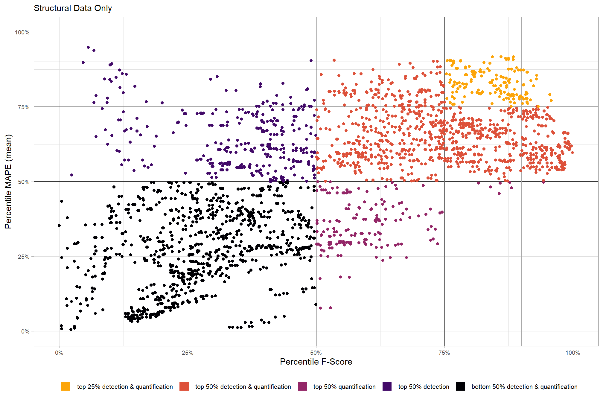
# param_combos_ranked %>% dplyr::count(is_final_selection)to determine the combinations that achieved the best balance between both detection and quantification accuracy, we’re selecting the parameter combinations that are in the upper-right of the quadrant plot. That is, the parameter combinations that performed best at both pile detection accuracy and pile form quantification accuracy
# plot
param_combos_ranked %>%
  ggplot2::ggplot(
    mapping=ggplot2::aes(x = ovrall_pct_rank_det_mean, y = ovrall_pct_rank_quant_mean, color = ovrall_accuracy_grp)
  ) +
  ggplot2::geom_vline(xintercept = 0.5, color = "gray22") +
  ggplot2::geom_hline(yintercept = 0.5, color = "gray22") +
  ggplot2::geom_vline(xintercept = 0.75, color = "gray44") +
  ggplot2::geom_hline(yintercept = 0.75, color = "gray44") +
  ggplot2::geom_vline(xintercept = 0.9, color = "gray66") +
  ggplot2::geom_hline(yintercept = 0.9, color = "gray66") +
  ggplot2::geom_point() +
  ggplot2::scale_colour_viridis_d(option = "inferno", end = 0.8, direction = -1) +
  ggplot2::scale_x_continuous(
    labels = scales::percent_format(accuracy = 1)
    , limits = c(0,1)
  ) +
  ggplot2::scale_y_continuous(
    labels = scales::percent_format(accuracy = 1)
    , limits = c(0,1)
  ) +
  ggplot2::labs(
    x = "Percentile F-Score", y = "Percentile MAPE (mean)"
    , color = ""
    , subtitle = "Structural Data Only"
  ) +
  ggplot2::theme_light() +
  ggplot2::theme(
    legend.position = "bottom"
    , legend.text = ggplot2::element_text(size = 8)
    , strip.text = ggplot2::element_text(size = 11, color = "black", face = "bold")
    , axis.text = ggplot2::element_text(size = 7)
  ) +
  ggplot2::guides(
    color = ggplot2::guide_legend(override.aes = list(shape = 15, linetype = 0, size = 5, alpha = 1))
    , shape = "none"
  )
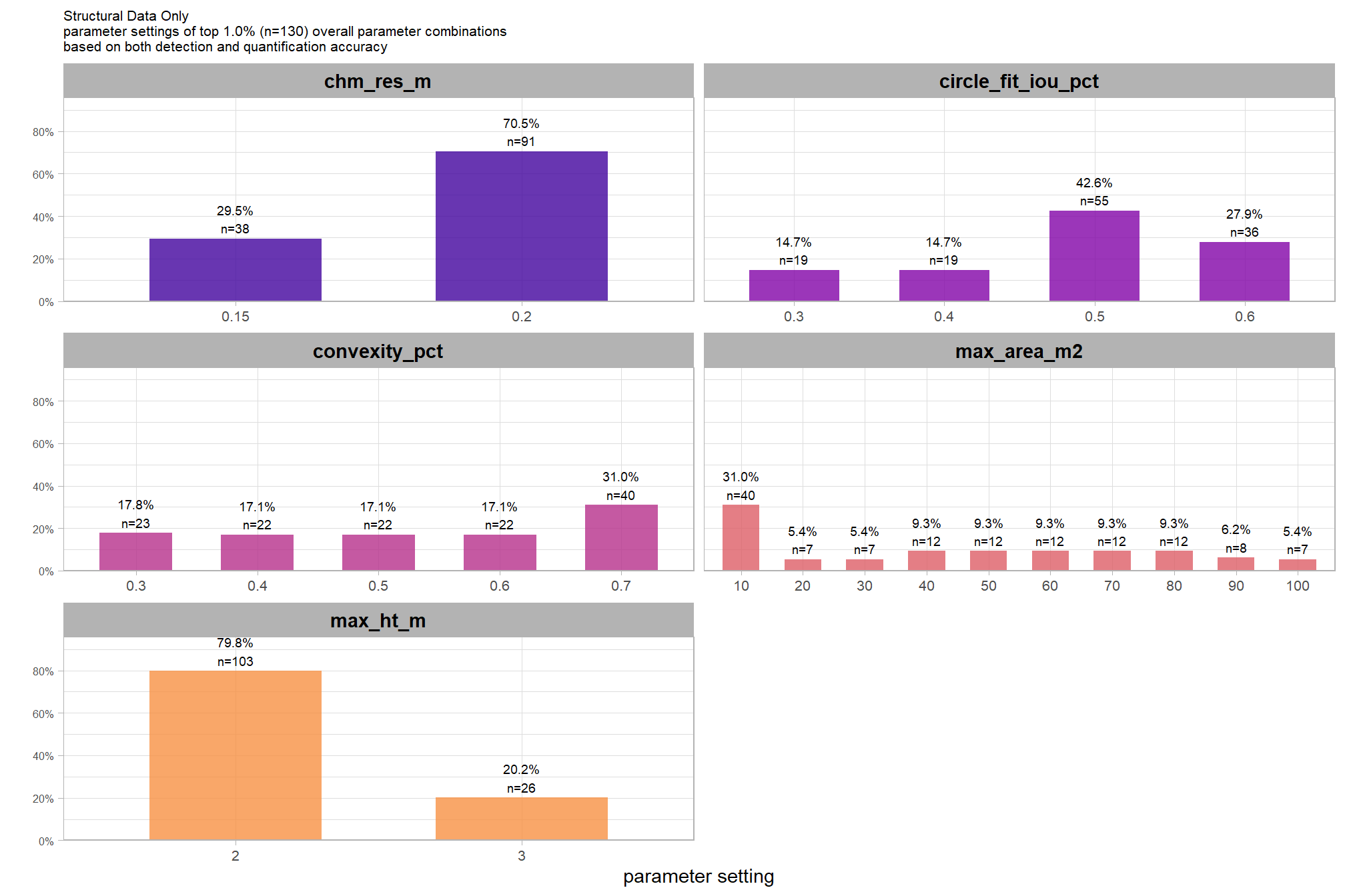
9.5.3.1.1 Top 1.0%
let’s check out the parameter settings of the top 1.0% (n=130) from all 12,960 combinations tested. these are “votes” for the parameter setting based on the combinations that achieved the best balance between both detection and quantification accuracy.
pal_param <- viridis::plasma(n=6, begin = 0.1, end = 0.9, alpha = 0.8)
param_combos_ranked %>%
  dplyr::filter(is_top_overall) %>%
  dplyr::select(tidyselect::contains("f_score"), max_ht_m,max_area_m2,convexity_pct,circle_fit_iou_pct,chm_res_m) %>%
  tidyr::pivot_longer(
    cols = c(max_ht_m,max_area_m2,convexity_pct,circle_fit_iou_pct,chm_res_m)
    , names_to = "metric"
    , values_to = "value"
  ) %>%
  dplyr::count(metric, value) %>%
  dplyr::group_by(metric) %>%
  dplyr::mutate(
    pct=n/sum(n)
    , lab = paste0(scales::percent(pct,accuracy=0.1), "\nn=", scales::comma(n,accuracy=1))
  ) %>%
  ggplot2::ggplot(
    mapping = ggplot2::aes(x = factor(value), y=pct, label=lab, fill = metric)
  ) +
  ggplot2::geom_col(width = 0.6) +
  ggplot2::geom_text(color = "black", size = 2.5, vjust = -0.2) +
  ggplot2::facet_wrap(facets = dplyr::vars(metric), ncol=2, scales = "free_x") +
  ggplot2::scale_y_continuous(
    breaks = seq(0,1,by=0.2)
    , labels = scales::percent
    , expand = ggplot2::expansion(mult = c(0,0.2))
  ) +
  ggplot2::scale_fill_manual(values = pal_param[1:5]) +
  ggplot2::labs(
    x = "parameter setting", y = ""
    , fill = ""
    , subtitle = paste0(
      "Structural Data Only"
       , "\nparameter settings of top "
       , scales::percent(pct_th_top,accuracy=0.1)
       , " (n="
       , scales::comma(n_combos_top_overall, accuracy = 1)
       , ") "
       , "overall parameter combinations\nbased on both detection and quantification accuracy"
    )
  ) +
  ggplot2::theme_light() +
  ggplot2::theme(
    legend.position = "none"
    , strip.text = ggplot2::element_text(size = 11, color = "black", face = "bold")
    , axis.text.y = ggplot2::element_text(size = 6)
    , axis.text.x = ggplot2::element_text(size = 8)
    , plot.subtitle = ggplot2::element_text(size = 8)
  )
what is the expected detection accuracy of the top 1.0% (n=130) combinations tested?
plt_detection_dist(
  df = param_combos_ranked %>% dplyr::filter(is_top_overall) %>% dplyr::select(!tidyselect::contains("_pct_rank_"))
  , paste0(
    "Structural Data Only"
    , "\ndistribution of evaluation metrics for top "
    , scales::percent(pct_th_top,accuracy=0.1)
    , " (n="
    , scales::comma(n_combos_top_overall, accuracy = 1)
    , ") "
    , "overall parameter combinations\nbased on both detection and quantification accuracy"
  )
)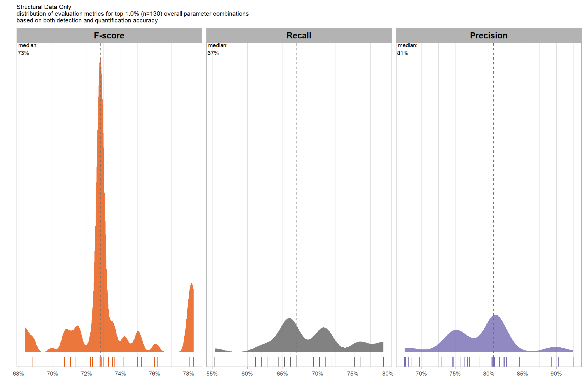
WHAT DID WE LEARN FROM THIS
what is the expected quantification accuracy of the top 1.0% (n=130) combinations tested?
# plot it
plt_form_quantification_dist(
  df = param_combos_ranked %>% dplyr::filter(is_top_overall) %>% dplyr::select(!tidyselect::contains("_pct_rank_"))
  , paste0(
    "Structural Data Only"
    , "\ndistribution of pile form quantification metrics for the top "
    , scales::percent(pct_th_top,accuracy=0.1)
    , " (n="
    , scales::comma(n_combos_top_overall, accuracy = 1)
    , ") "
    , "overall parameter combinations\nbased on both detection and quantification accuracy"
  )
)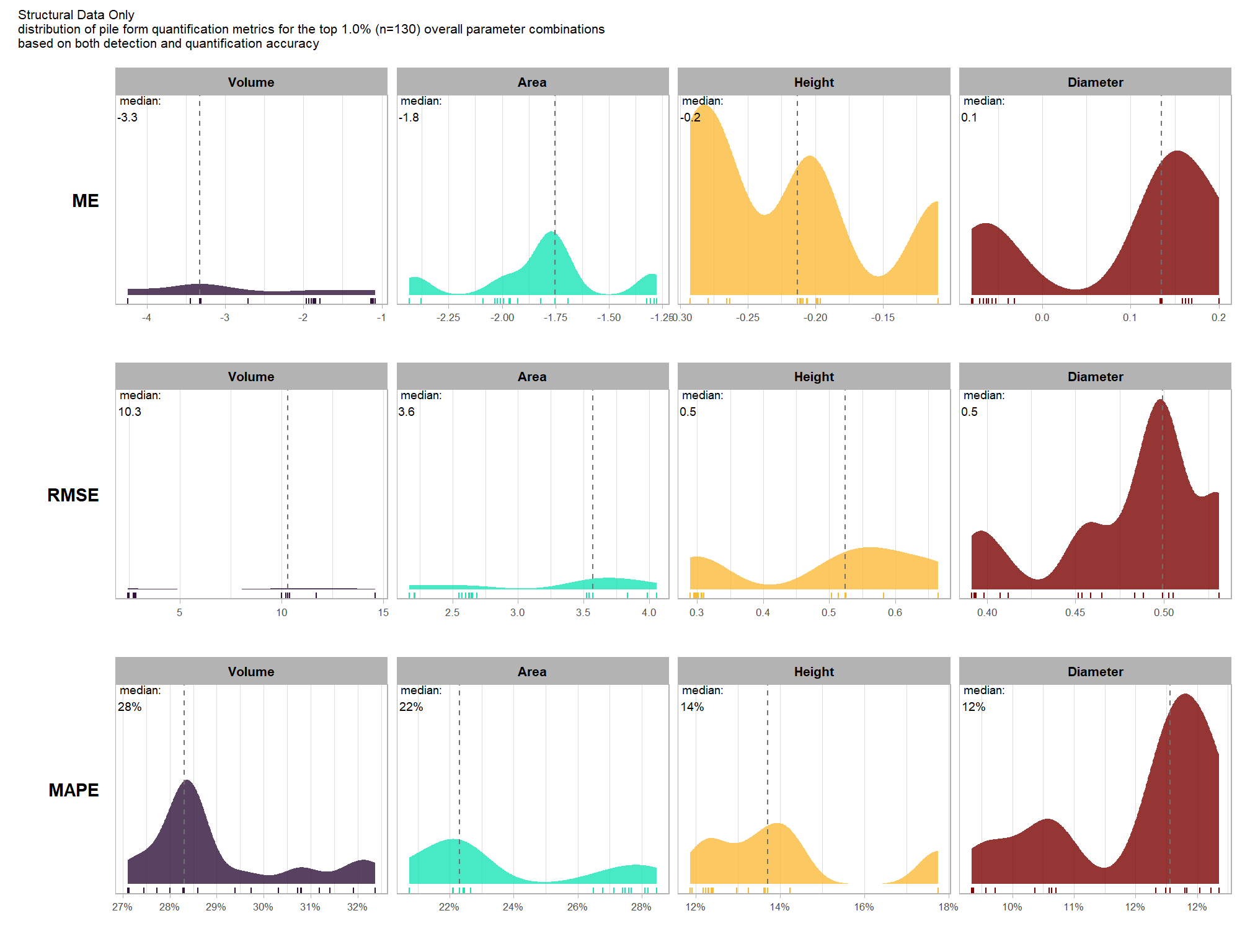
WHAT DID WE LEARN FROM THIS
9.5.3.1.2 Final 12 recommended settings
# pal_temp %>% scales::show_col()
# filter and reshape
param_combos_ranked %>%
  dplyr::filter(is_final_selection) %>%
  dplyr::select(!tidyselect::contains("_pct_rank_")) %>%
  dplyr::select(
    max_ht_m,max_area_m2,convexity_pct,circle_fit_iou_pct,chm_res_m
    , ovrall_lab
    # detection
    , f_score, recall, precision
    # quantification
    , tidyselect::ends_with("_rmse")
    , tidyselect::ends_with("_rrmse")
    , tidyselect::ends_with("_mean")
    , tidyselect::ends_with("_mape")
  ) %>%
  tidyr::pivot_longer(
    cols = c(
      f_score, recall, precision
      , tidyselect::ends_with("_rmse")
      , tidyselect::ends_with("_rrmse")
      , tidyselect::ends_with("_mean")
      , tidyselect::ends_with("_mape")
    )
    , names_to = "metric"
    , values_to = "value"
  ) %>%
  dplyr::mutate(
    eval_metric = stringr::str_extract(metric, "(_rmse|_rrmse|_mean|_mape|f_score|recall|precision)$") %>%
      stringr::str_remove_all("_") %>%
      stringr::str_replace_all("mean","me") %>%
      toupper() %>%
      factor(
        ordered = T
        , levels = c("FSCORE","RECALL","PRECISION", "ME","RMSE","RRMSE","MAPE")
        , labels = c("F-score","Recall","Precision", "ME","RMSE","RRMSE","MAPE")
      )
    , pile_metric = metric %>%
      stringr::str_remove("(_rmse|_rrmse|_mean|_mape)$") %>%
      stringr::str_extract("(paraboloid_volume|volume|area|height|diameter)") %>%
      dplyr::coalesce("detection") %>%
      factor(
        ordered = T
        , levels = c(
          "detection"
          , "volume"
          , "paraboloid_volume"
          , "area"
          , "height"
          , "diameter"
        )
        , labels = c(
          "Detection"
          , "Volume"
          , "Volume paraboloid"
          , "Area"
          , "Height"
          , "Diameter"
        )
      )
    , value_lab = dplyr::case_when(
        eval_metric %in% c("F-score","Recall","Precision", "RRMSE", "MAPE") ~ scales::percent(value,accuracy=0.1)
        , eval_metric == "ME" ~ scales::comma(value,accuracy=0.01)
        , T ~ scales::comma(value,accuracy=0.1)
      )
  ) %>%
  # make var for color
  dplyr::group_by(pile_metric, eval_metric) %>%
  dplyr::mutate(
    # for ME, color by abs...for f-score,recall,precision color by -value so that higher means better...
      # ...since higher means worse for quantification accuracy metrics
    value_dir = dplyr::case_when(
      eval_metric %in% c("ME") ~ abs(value)
      , eval_metric %in% c("F-score","Recall","Precision") ~ -value
      , T ~ value
    )
    , value_z = (value_dir-mean(value_dir,na.rm=T))/sd(value_dir,na.rm=T) # this is the key to the different colors within facets
  ) %>%
  dplyr::ungroup() %>%
  dplyr::filter(!eval_metric %in% c("RRMSE")) %>%
  # View()
  ggplot2::ggplot(mapping = ggplot2::aes(x = eval_metric, y = ovrall_lab)) +
  ggplot2::geom_tile(
    mapping = ggplot2::aes(fill = pile_metric, alpha = -value_z)
    , color = "gray"
  ) +
  ggplot2::geom_text(
    mapping = ggplot2::aes(label = value_lab, fontface = "bold")
    , color = "white"
  ) +
  ggplot2::facet_grid(cols = dplyr::vars(pile_metric), scales = "free_x") +
  ggplot2::scale_x_discrete(position = "top") +
  ggplot2::scale_fill_manual(values = c("gray33", viridis::turbo(n=4))) +
  ggplot2::scale_alpha_binned(range = c(0.55, 1)) + # this is the key to the different colors within facets
  ggplot2::theme_light() +
  ggplot2::labs(
    x = ""
    , y = "max_ht_m : max_area_m2 : convexity_pct : circle_fit_iou_pct : chm_res_m"
    , subtitle = paste0(
       "Structural Data Only"
       , "\npile detection and form quantification accuracy metrics for the final recommended parameter settings"
       # , scales::percent(1-pct_rank_th_top,accuracy=1)
       , " (n="
       , scales::comma(n_th_top,accuracy=1)
       , ") "
       , "\nbased on both detection and quantification accuracy"
      )
    , caption = "*darker colors indicate relatively higher accuracy values"
  ) +
  ggplot2::theme(

    legend.position = "none"
    , panel.grid = ggplot2::element_blank()
    , strip.placement = "outside"
    , strip.text.x = ggplot2::element_text(size = 8, color = "black", face = "bold")
    , axis.text.x = ggplot2::element_text(size = 7, color = "black", face = "bold")
    , axis.title.x = ggplot2::element_blank()
    , plot.subtitle = ggplot2::element_text(size = 8)
  )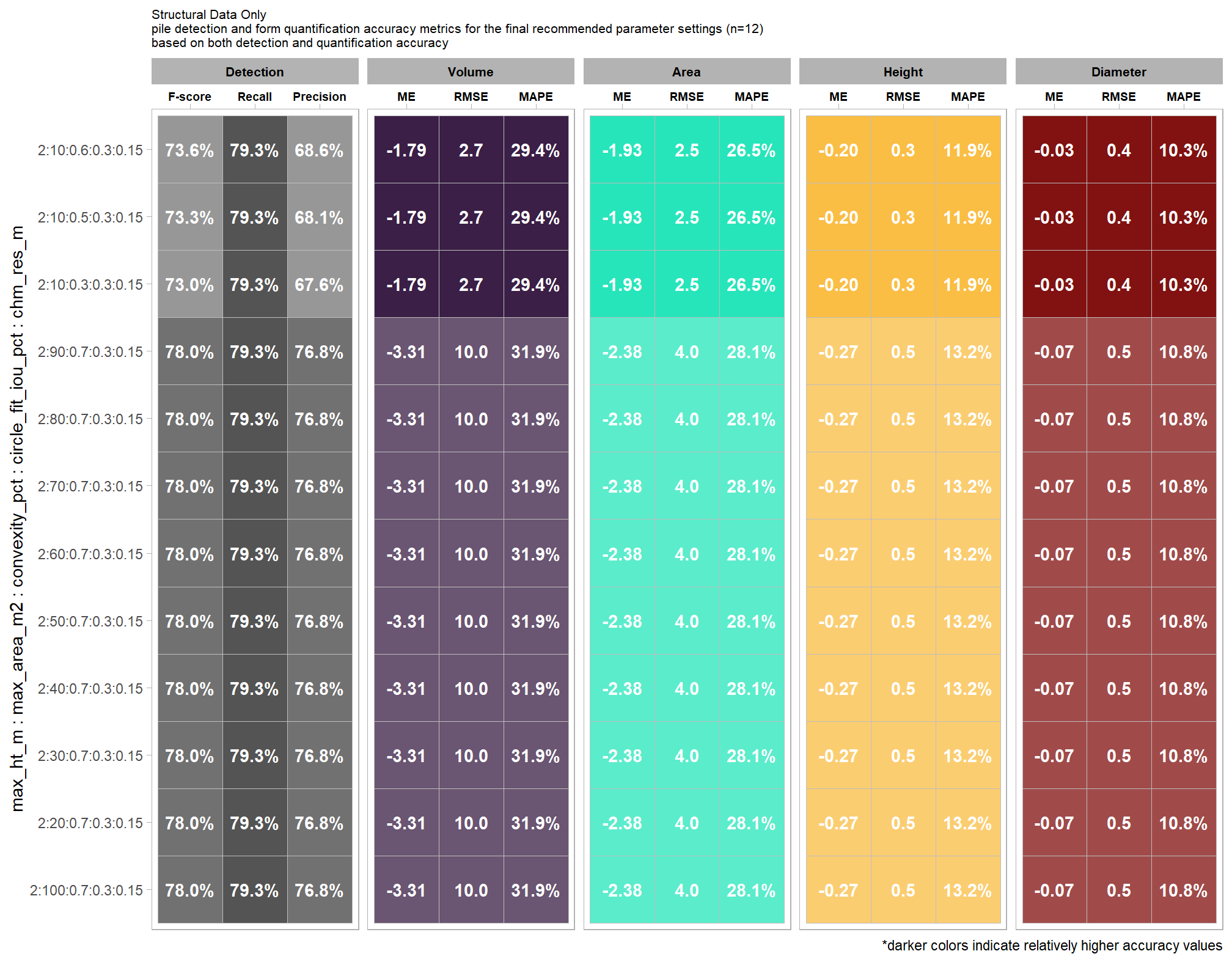
this plot allows for a simultaneous comparison of all metrics for pile detection and pile form quantification. it includes only the parameter combinations that achieved the best balanced accuracy, helping users identify the optimal settings by evaluating the trade-offs between detection and form quantification.
let’s table this
param_combos_ranked %>%
  dplyr::filter(is_final_selection) %>%
  dplyr::select(!tidyselect::contains("_pct_rank_")) %>%
  # first select to arrange eval_metric
  dplyr::select(
    ovrall_lab
    , max_ht_m,max_area_m2,convexity_pct,circle_fit_iou_pct,chm_res_m
    # detection
    , f_score, recall, precision
    # quantification
    , tidyselect::ends_with("_mean")
    , tidyselect::ends_with("_rmse")
    # , tidyselect::ends_with("_rrmse")
    , tidyselect::ends_with("_mape")
  ) %>%
  # second select to arrange pile_metric
  dplyr::select(
    ovrall_lab
    , max_ht_m,max_area_m2,convexity_pct,circle_fit_iou_pct,chm_res_m
    # detection
    , f_score, recall, precision
    # quantification
    , c(tidyselect::contains("volume") & !tidyselect::contains("paraboloid"))
    , tidyselect::contains("area")
    , tidyselect::contains("height")
    , tidyselect::contains("diameter")
  ) %>%
  # names()
  dplyr::mutate(
    dplyr::across(
      .cols = c(f_score, recall, precision, tidyselect::ends_with("_mape"))
      , .fn = ~ scales::percent(.x, accuracy = 1)
    )
    , dplyr::across(
      .cols = c(tidyselect::ends_with("_mean"))
      , .fn = ~ scales::comma(.x, accuracy = 0.01)
    )
    , dplyr::across(
      .cols = c(tidyselect::ends_with("_rmse"))
      , .fn = ~ scales::comma(.x, accuracy = 0.1)
    )
  ) %>%
  dplyr::mutate(blank= "   " ) %>%
  dplyr::relocate(blank, .before = f_score) %>%
  dplyr::arrange(desc(ovrall_lab)) %>%
  kableExtra::kbl(
    caption =
      paste0(
       "Structural Data Only"
       , "<br>pile detection and form quantification accuracy metrics for the final recommended parameter settings"
       # , scales::percent(1-pct_rank_th_top,accuracy=1)
       , " (n="
       , scales::comma(n_th_top,accuracy=1)
       , ") "
       , "<br>based on both detection and quantification accuracy"
      )
    , col.names = c(
      ""
      ,"max_ht_m","max_area_m2","convexity_pct","circle_fit_iou_pct","chm_res_m"
      , "   "
      , "F-score", "Recall", "Precision"
      , rep(c("ME","RMSE","MAPE"), times = 4)
    )
    , escape = F
  ) %>%
  kableExtra::kable_styling(font_size = 11) %>%
  kableExtra::add_header_above(c(
    " "=7
    , "Detection" = 3
    , "Volume" = 3
    , "Area" = 3
    , "Height" = 3
    , "Diameter" = 3
  )) %>%
  kableExtra::column_spec(seq(7,22,by=3), border_right = TRUE, include_thead = TRUE) %>%
  kableExtra::column_spec(
    column = 7:22
    , extra_css = "font-size: 10px;"
    , include_thead = T
  ) %>%
kableExtra::scroll_box(width = "740px") | max_ht_m | max_area_m2 | convexity_pct | circle_fit_iou_pct | chm_res_m | F-score | Recall | Precision | ME | RMSE | MAPE | ME | RMSE | MAPE | ME | RMSE | MAPE | ME | RMSE | MAPE | ||
|---|---|---|---|---|---|---|---|---|---|---|---|---|---|---|---|---|---|---|---|---|---|
| 2:10:0.6:0.3:0.15 | 2 | 10 | 0.6 | 0.3 | 0.15 | 74% | 79% | 69% | -1.79 | 2.7 | 29% | -1.93 | 2.5 | 26% | -0.20 | 0.3 | 12% | -0.03 | 0.4 | 10% | |
| 2:10:0.5:0.3:0.15 | 2 | 10 | 0.5 | 0.3 | 0.15 | 73% | 79% | 68% | -1.79 | 2.7 | 29% | -1.93 | 2.5 | 26% | -0.20 | 0.3 | 12% | -0.03 | 0.4 | 10% | |
| 2:10:0.3:0.3:0.15 | 2 | 10 | 0.3 | 0.3 | 0.15 | 73% | 79% | 68% | -1.79 | 2.7 | 29% | -1.93 | 2.5 | 26% | -0.20 | 0.3 | 12% | -0.03 | 0.4 | 10% | |
| 2:90:0.7:0.3:0.15 | 2 | 90 | 0.7 | 0.3 | 0.15 | 78% | 79% | 77% | -3.31 | 10.0 | 32% | -2.38 | 4.0 | 28% | -0.27 | 0.5 | 13% | -0.07 | 0.5 | 11% | |
| 2:80:0.7:0.3:0.15 | 2 | 80 | 0.7 | 0.3 | 0.15 | 78% | 79% | 77% | -3.31 | 10.0 | 32% | -2.38 | 4.0 | 28% | -0.27 | 0.5 | 13% | -0.07 | 0.5 | 11% | |
| 2:70:0.7:0.3:0.15 | 2 | 70 | 0.7 | 0.3 | 0.15 | 78% | 79% | 77% | -3.31 | 10.0 | 32% | -2.38 | 4.0 | 28% | -0.27 | 0.5 | 13% | -0.07 | 0.5 | 11% | |
| 2:60:0.7:0.3:0.15 | 2 | 60 | 0.7 | 0.3 | 0.15 | 78% | 79% | 77% | -3.31 | 10.0 | 32% | -2.38 | 4.0 | 28% | -0.27 | 0.5 | 13% | -0.07 | 0.5 | 11% | |
| 2:50:0.7:0.3:0.15 | 2 | 50 | 0.7 | 0.3 | 0.15 | 78% | 79% | 77% | -3.31 | 10.0 | 32% | -2.38 | 4.0 | 28% | -0.27 | 0.5 | 13% | -0.07 | 0.5 | 11% | |
| 2:40:0.7:0.3:0.15 | 2 | 40 | 0.7 | 0.3 | 0.15 | 78% | 79% | 77% | -3.31 | 10.0 | 32% | -2.38 | 4.0 | 28% | -0.27 | 0.5 | 13% | -0.07 | 0.5 | 11% | |
| 2:30:0.7:0.3:0.15 | 2 | 30 | 0.7 | 0.3 | 0.15 | 78% | 79% | 77% | -3.31 | 10.0 | 32% | -2.38 | 4.0 | 28% | -0.27 | 0.5 | 13% | -0.07 | 0.5 | 11% | |
| 2:20:0.7:0.3:0.15 | 2 | 20 | 0.7 | 0.3 | 0.15 | 78% | 79% | 77% | -3.31 | 10.0 | 32% | -2.38 | 4.0 | 28% | -0.27 | 0.5 | 13% | -0.07 | 0.5 | 11% | |
| 2:100:0.7:0.3:0.15 | 2 | 100 | 0.7 | 0.3 | 0.15 | 78% | 79% | 77% | -3.31 | 10.0 | 32% | -2.38 | 4.0 | 28% | -0.27 | 0.5 | 13% | -0.07 | 0.5 | 11% |
what is the expected detection accuracy of the final 12 recommended settings?
plt_detection_dist(
  df = param_combos_ranked %>% dplyr::filter(is_final_selection) %>% dplyr::select(!tidyselect::contains("_pct_rank_"))
  , paste0(
    "Structural Data Only"
    , "\ndistribution of evaluation metrics for the final recommended parameter settings"
    , " (n="
    , scales::comma(n_th_top,accuracy=1)
    , ") "
    , "\nbased on both detection and quantification accuracy"
  )
)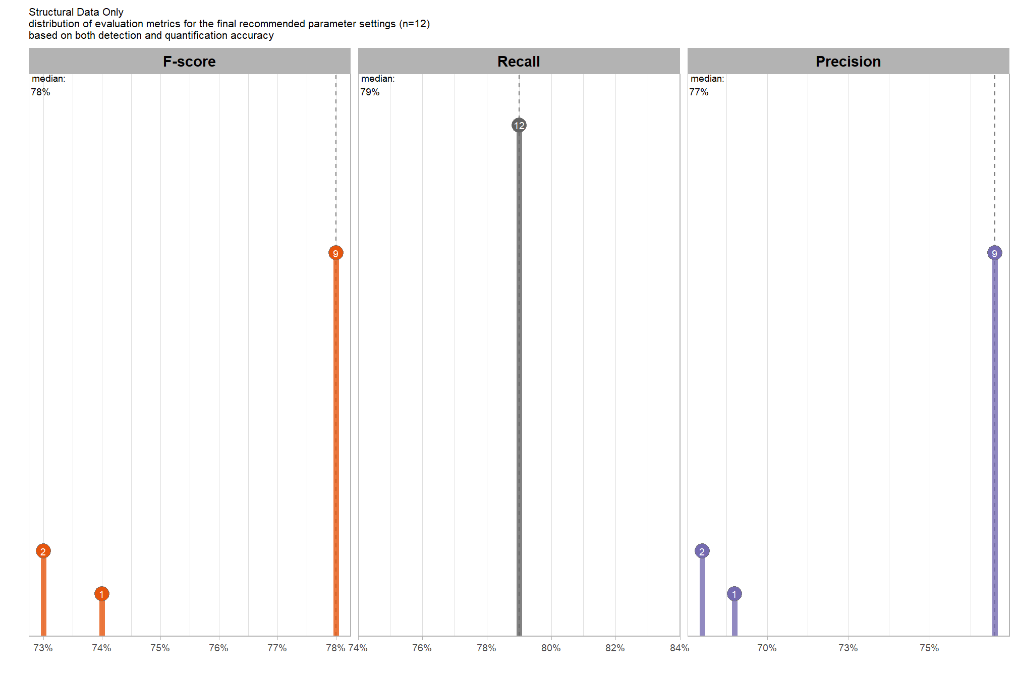
WHAT DID WE LEARN FROM THIS
what is the expected quantification accuracy of the final 12 recommended settings?
# plot it
plt_form_quantification_dist(
  df = param_combos_ranked %>% dplyr::filter(is_final_selection) %>% dplyr::select(!tidyselect::contains("_pct_rank_"))
  , paste0(
    "Structural Data Only"
    , "\ndistribution of pile form quantification metrics for the final recommended parameter settings"
    , " (n="
    , scales::comma(n_th_top,accuracy=1)
    , ") "
    , "\nbased on both detection and quantification accuracy"
  )
)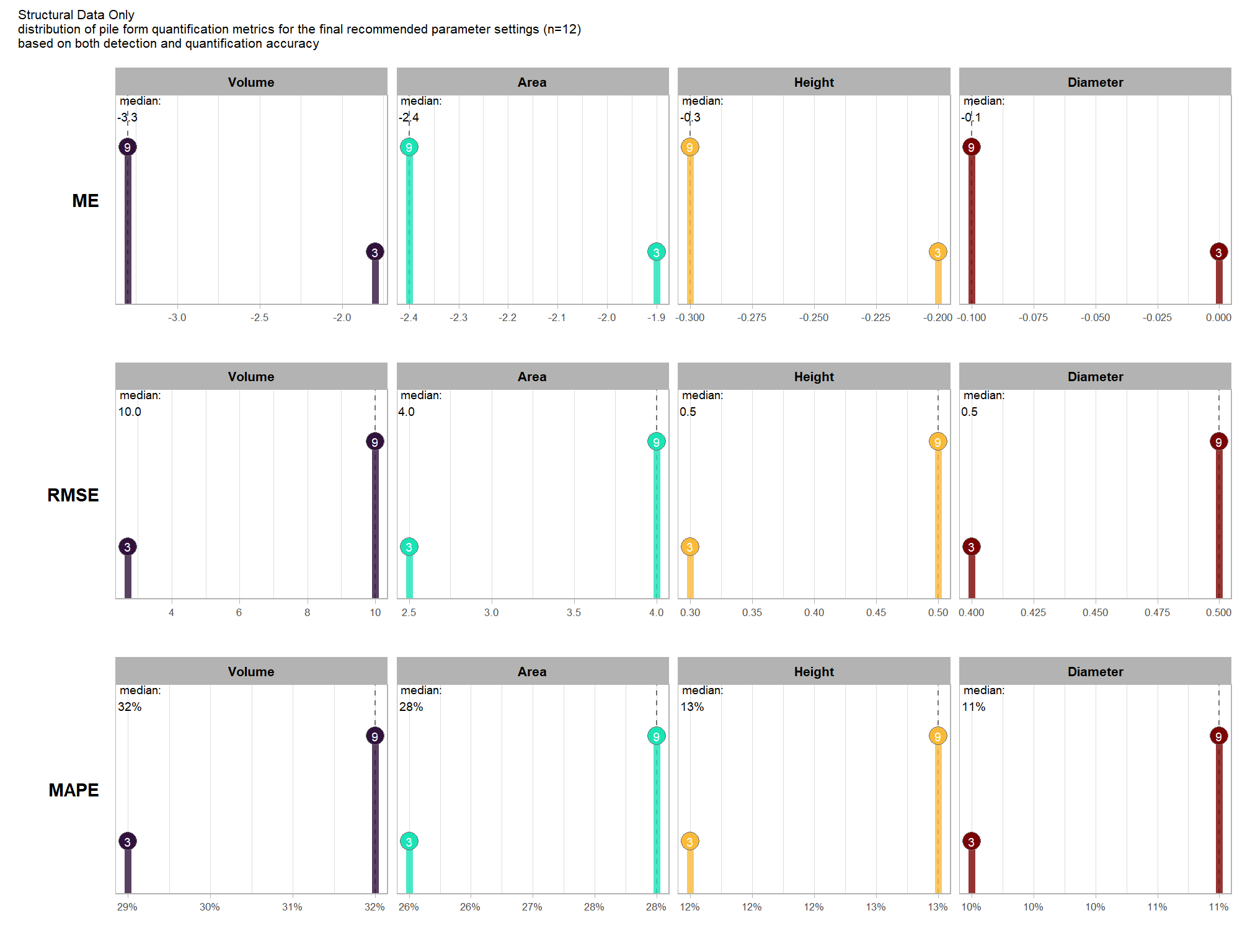
WHAT DID WE LEARN FROM THIS
finally, here are the combinations selected compared against all 12,960 combinations tested.
param_combos_ranked %>%
  dplyr::select(
    rn,max_ht_m,max_area_m2,convexity_pct,circle_fit_iou_pct
    , is_final_selection
    , f_score, precision, recall
    # quantification accuracy
    , tidyselect::ends_with("_mape")
  ) %>%
  tidyr::pivot_longer(
    cols = c(
      tidyselect::ends_with("_mape")
      # ,precision,recall
    )
    , names_to = "metric"
    , values_to = "value"
  ) %>%
  dplyr::mutate(
    eval_metric = stringr::str_extract(metric, "(_rmse|_rrmse|_mean|_mape)$") %>%
      stringr::str_remove_all("_") %>%
      stringr::str_replace_all("mean","me") %>%
      toupper() %>%
      factor(
        ordered = T
        , levels = c("ME","RMSE","RRMSE","MAPE")
      )
    , pile_metric = metric %>%
      stringr::str_remove("(_rmse|_rrmse|_mean|_mape)$") %>%
      stringr::str_extract("(paraboloid_volume|volume|area|height|diameter|precision|recall)") %>%
      factor(
        ordered = T
        , levels = c(
          "volume"
          , "paraboloid_volume"
          , "area"
          , "height"
          , "diameter"
          , "recall"
          , "precision"
        )
        , labels = c(
          "Volume"
          , "Volume paraboloid"
          , "Area"
          , "Height"
          , "Diameter"
          , "Recall"
          , "Precision"
        )
      )
    , color_metric = ifelse(is_final_selection, pile_metric, NA) %>% factor()
  ) %>%
  dplyr::arrange(is_final_selection) %>%
  # plot
  ggplot2::ggplot(mapping = ggplot2::aes(x = f_score, y = value, color = color_metric)) +
  ggplot2::geom_point() +
  ggplot2::facet_wrap(facets = dplyr::vars(pile_metric)) +
  ggplot2::scale_color_viridis_d(option = "turbo", na.value = "gray88") +
  ggplot2::scale_x_continuous(
    labels = scales::percent_format(accuracy = 1)
    , limits = c(0,1)
  ) +
  ggplot2::scale_y_continuous(
    labels = scales::percent_format(accuracy = 1)
    , limits = c(0,NA)
  ) +
  ggplot2::labs(x = "F-Score", y = "MAPE", caption = "*records in gray not selected") +
  ggplot2::theme_light() +
  ggplot2::theme(
    legend.position = "none"
    , strip.text = ggplot2::element_text(size = 11, color = "black", face = "bold")
  )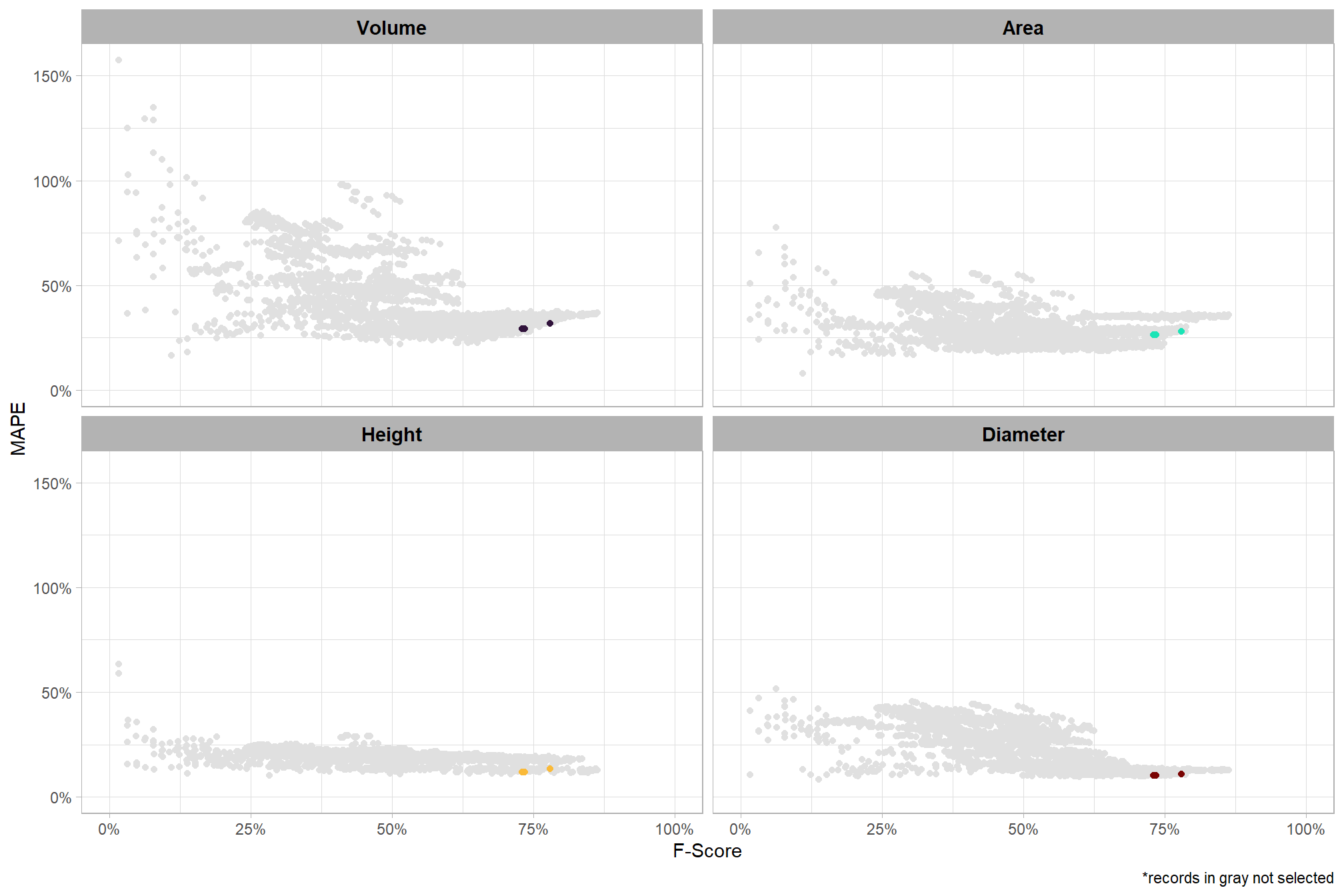
WHAT DID WE LEARN FROM THIS
9.5.3.2 by CHM resolution
To select the best-performing parameter combinations, we will prioritize those that balance detection and quantification accuracy. From this group, we will then identify the settings that achieve the highest pile detection rates (recall). These recommendations are for users who are working with a CHM with a resolution in the range of those tested for this analysis or can aggregate (i.e. make more coarse) a CHM to a resolution tested for the purpose of either improving processing performance or enhancing pile detection and/or quantification accuracy based on the results shown here
we already created this data above (param_combos_ranked) using the F-Score and the average rank of the MAPE metrics across all form measurements (i.e. height, diameter, area, volume) to determine the best overall list by CHM resolution
9.5.3.2.1 Top 2.0%
let’s check out the parameter settings of the top 2.0% (n=28) from all 1,440 combinations tested by CHM resolution. these are “votes” for the parameter setting based on the combinations that achieved the best balance between both detection and quantification accuracy.
param_combos_ranked %>%
  dplyr::filter(is_top_chm) %>%
  dplyr::select(tidyselect::contains("f_score"), max_ht_m,max_area_m2,convexity_pct,circle_fit_iou_pct,chm_res_m,chm_res_m_desc) %>%
  tidyr::pivot_longer(
    cols = c(max_ht_m,max_area_m2,convexity_pct,circle_fit_iou_pct)
    , names_to = "metric"
    , values_to = "value"
  ) %>%
  dplyr::count(chm_res_m,chm_res_m_desc, metric, value) %>%
  dplyr::group_by(chm_res_m,chm_res_m_desc, metric) %>%
  dplyr::mutate(
    pct=n/sum(n)
    , lab = paste0(scales::percent(pct,accuracy=0.1)) #, "\nn=", scales::comma(n,accuracy=1))
  ) %>%
  ggplot2::ggplot(
    mapping = ggplot2::aes(x = factor(value), y=pct, label=lab, fill = metric)
  ) +
  ggplot2::geom_col(width = 0.6) +
  ggplot2::geom_text(color = "black", size = 2.2, vjust = -0.2) +
  ggplot2::facet_grid(cols = dplyr::vars(metric), rows = dplyr::vars(chm_res_m_desc), scales = "free_x") +
  ggplot2::scale_y_continuous(
    breaks = seq(0,1,by=0.2)
    , labels = scales::percent
    , expand = ggplot2::expansion(mult = c(0,0.2))
  ) +
  ggplot2::scale_fill_manual(values = pal_param[1:4]) +
  ggplot2::labs(
    x = "parameter setting", y = ""
    , fill = ""
    , subtitle = paste0(
      "Structural Data Only"
       , "\nparameter settings of top "
       , scales::percent(pct_th_top_chm,accuracy=0.1)
       , " (n="
       , scales::comma(n_combos_top_chm , accuracy = 1)
       , ") "
       , "parameter combinations by CHM resolution\nbased on both detection and quantification accuracy"
    )
  ) +
  ggplot2::theme_light() +
  ggplot2::theme(
    legend.position = "none"
    , strip.text.x = ggplot2::element_text(size = 11, color = "black", face = "bold")
    , strip.text.y = ggplot2::element_text(size = 9, color = "black", face = "bold")
    , axis.text.y = ggplot2::element_text(size = 6)
    , axis.text.x = ggplot2::element_text(size = 8)
    , plot.subtitle = ggplot2::element_text(size = 8)
  )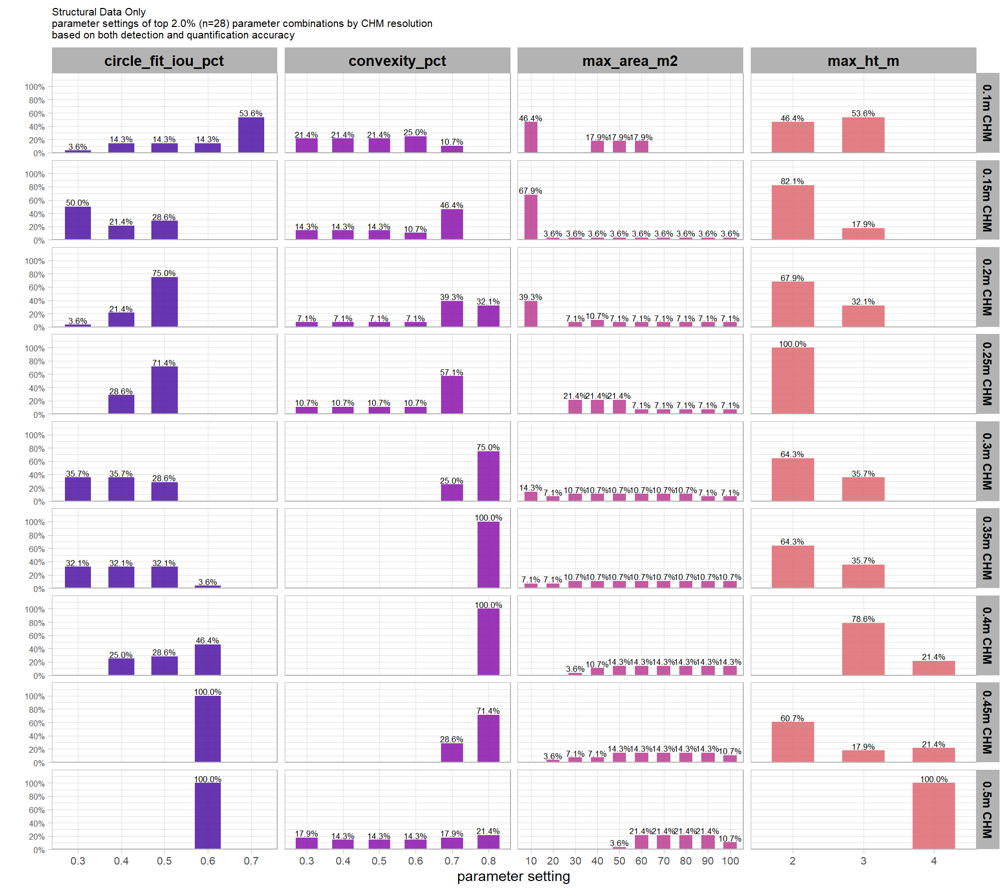
what is the expected detection accuracy of the top 2.0% (n=28) combinations tested by CHM resolution?
plt_detection_dist2(
  df = param_combos_ranked %>% dplyr::filter(is_top_chm) %>% dplyr::select(!tidyselect::contains("_pct_rank_"))
  , paste0(
    "Structural Data Only"
    , "\ndistribution of evaluation metrics for top "
    , scales::percent(pct_th_top_chm,accuracy=0.1)
    , " (n="
    , scales::comma(n_combos_top_chm, accuracy=1)
    , ") "
    , "parameter combinations by CHM resolution\nbased on both detection and quantification accuracy"
  )
)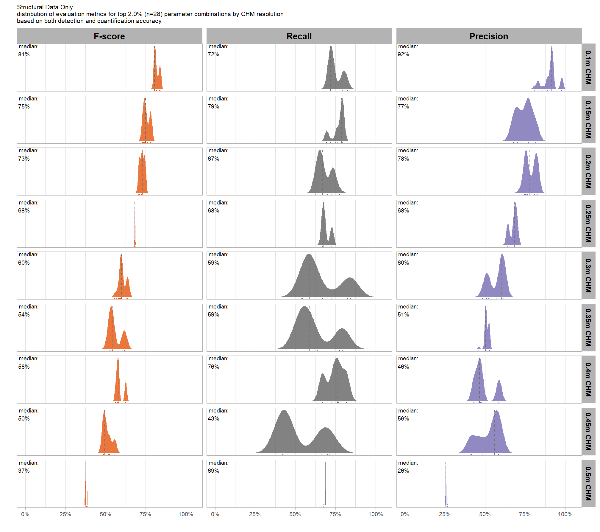
WHAT DID WE LEARN FROM THIS
what is the expected MAPE of the top 2.0% (n=28) combinations tested by CHM resolution?
# plot it
plt_form_quantification_dist2(
  df = param_combos_ranked %>% dplyr::filter(is_top_chm) %>% dplyr::select(!tidyselect::contains("_pct_rank_"))
  , quant_metric = "mape"
  , paste0(
    "Structural Data Only"
    , "\ndistribution of pile form quantification metrics for the top "
    , scales::percent(pct_th_top_chm,accuracy=0.1)
    , " (n="
    , scales::comma(n_combos_top_chm, accuracy=1)
    , ") "
    , "parameter combinations by CHM resolution\nbased on both detection and quantification accuracy"
  )
)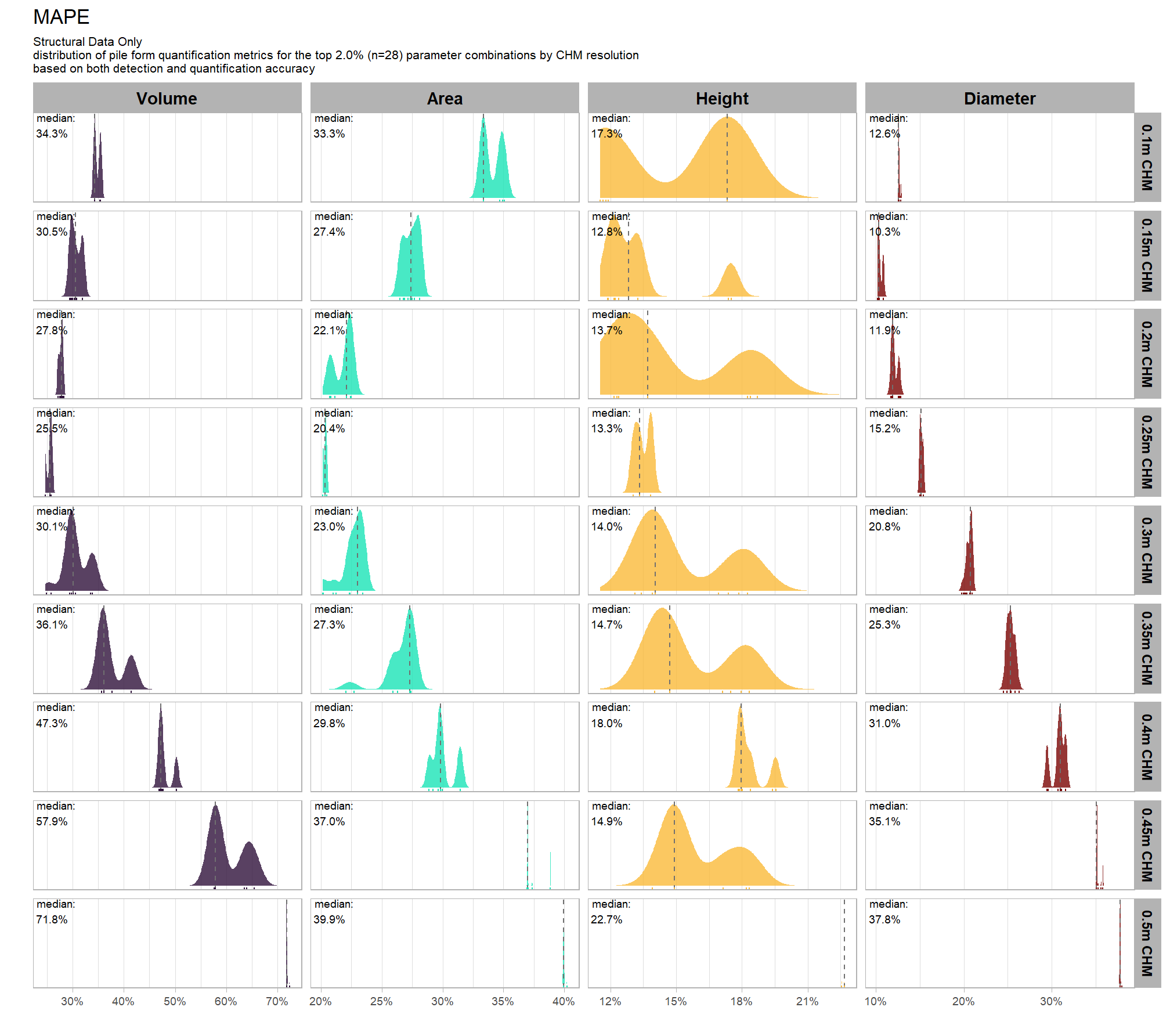
WHAT DID WE LEARN FROM THIS
what is the expected Mean Error (ME) of the top 2.0% (n=28) combinations tested by CHM resolution?
# plot it
plt_form_quantification_dist2(
  df = param_combos_ranked %>% dplyr::filter(is_top_chm) %>% dplyr::select(!tidyselect::contains("_pct_rank_"))
  , quant_metric = "mean"
  , paste0(
    "Structural Data Only"
    , "\ndistribution of pile form quantification metrics for the top "
    , scales::percent(pct_th_top_chm,accuracy=0.1)
    , " (n="
    , scales::comma(n_combos_top_chm, accuracy=1)
    , ") "
    , "parameter combinations by CHM resolution\nbased on both detection and quantification accuracy"
  )
)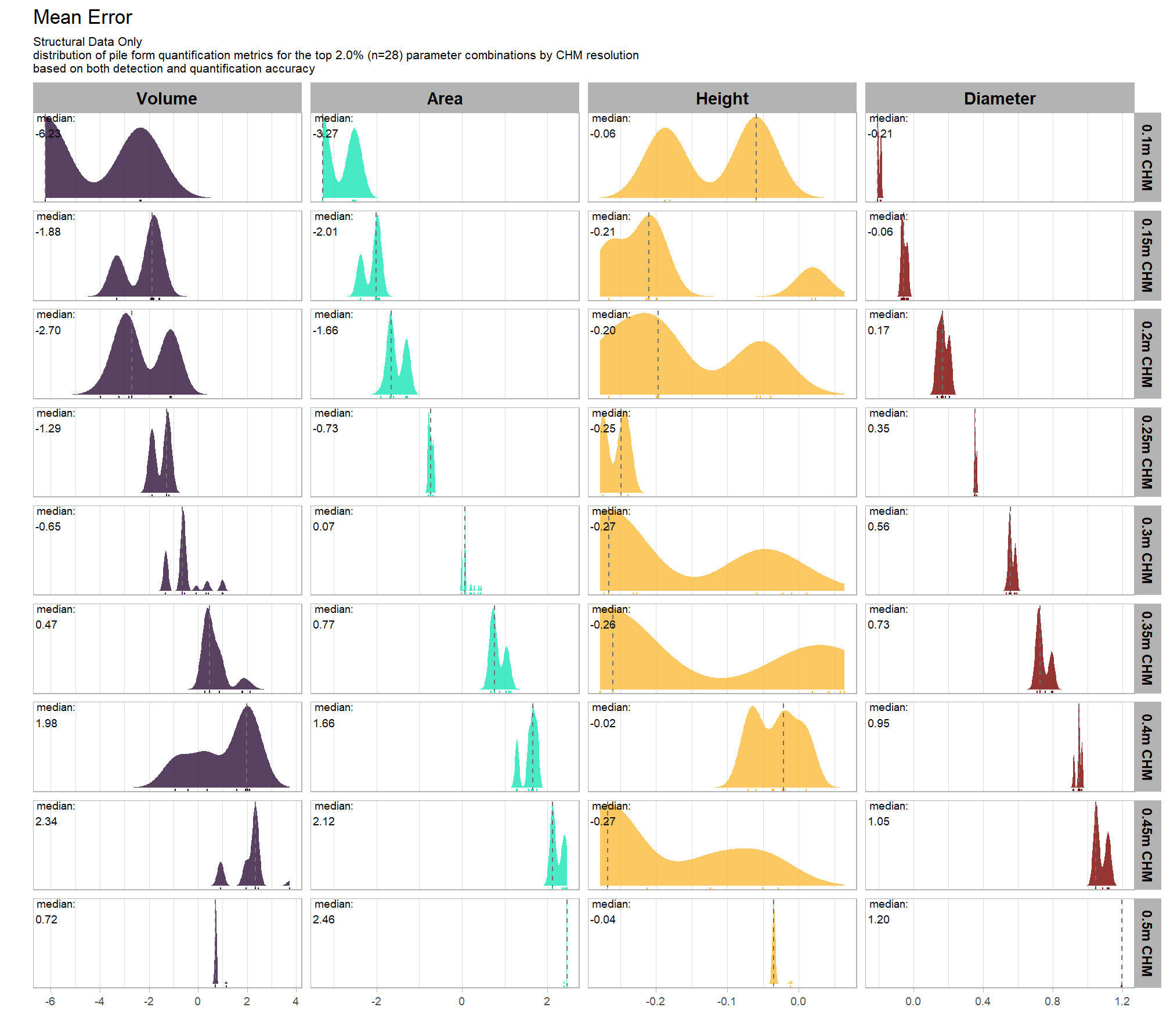
WHAT DID WE LEARN FROM THIS
what is the expected RMSE of the top 2.0% (n=28) combinations tested by CHM resolution?
# plot it
plt_form_quantification_dist2(
  df = param_combos_ranked %>% dplyr::filter(is_top_chm) %>% dplyr::select(!tidyselect::contains("_pct_rank_"))
  , quant_metric = "rmse"
  , paste0(
    "Structural Data Only"
    , "\ndistribution of pile form quantification metrics for the top "
    , scales::percent(pct_th_top_chm,accuracy=0.1)
    , " (n="
    , scales::comma(n_combos_top_chm, accuracy=1)
    , ") "
    , "parameter combinations by CHM resolution\nbased on both detection and quantification accuracy"
  )
)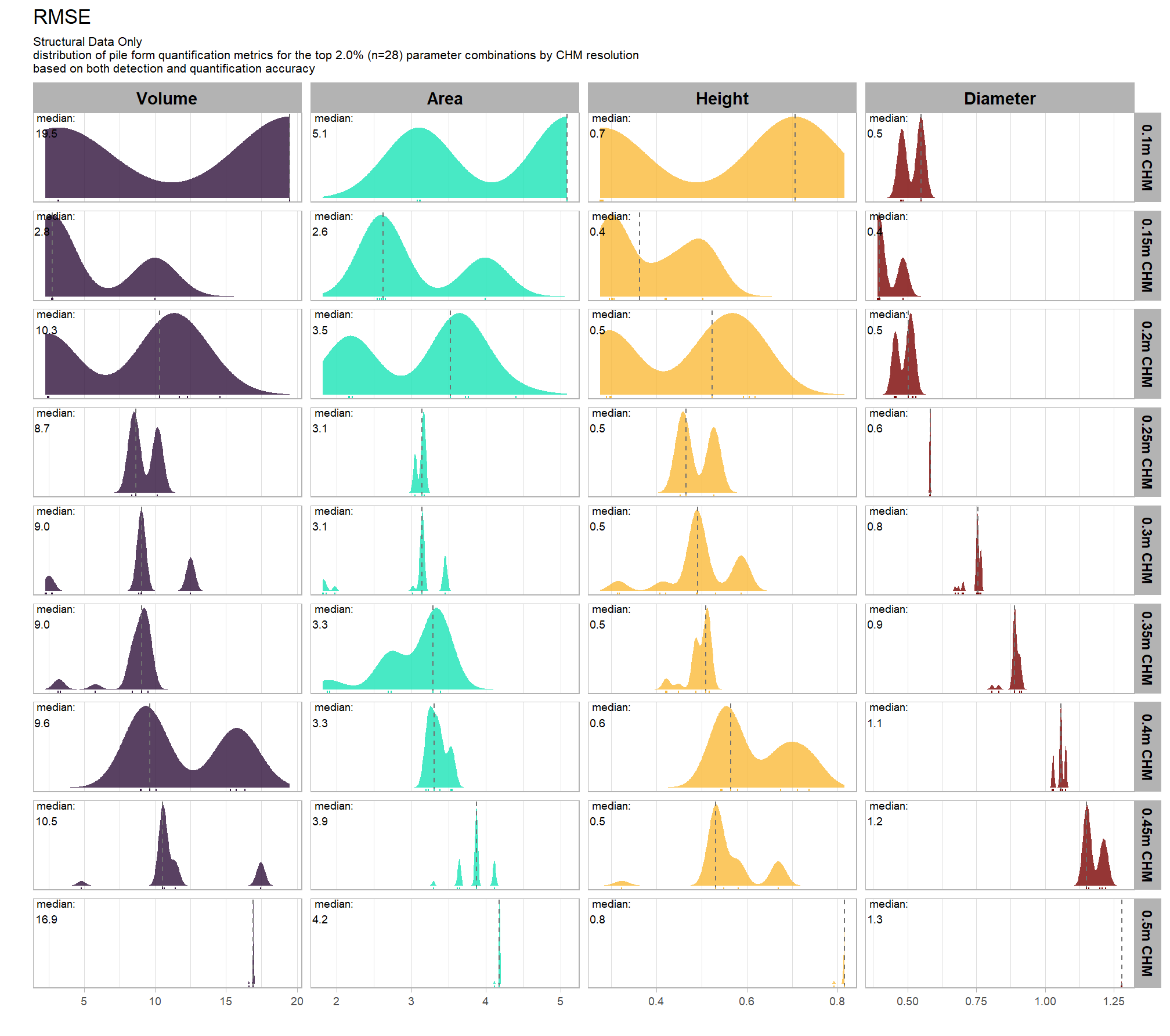
WHAT DID WE LEARN FROM THIS
9.5.3.2.2 Final 6 recommended settings
# pal_temp %>% scales::show_col()
# filter and reshape
param_combos_ranked %>%
  dplyr::filter(is_final_selection_chm) %>%
  dplyr::select(!tidyselect::contains("_pct_rank_")) %>%
  dplyr::select(
    max_ht_m,max_area_m2,convexity_pct,circle_fit_iou_pct,chm_res_m,chm_res_m_desc
    , chm_lab
    # detection
    , f_score, recall, precision
    # quantification
    , tidyselect::ends_with("_rmse")
    , tidyselect::ends_with("_rrmse")
    , tidyselect::ends_with("_mean")
    , tidyselect::ends_with("_mape")
  ) %>%
  tidyr::pivot_longer(
    cols = c(
      f_score, recall, precision
      , tidyselect::ends_with("_rmse")
      , tidyselect::ends_with("_rrmse")
      , tidyselect::ends_with("_mean")
      , tidyselect::ends_with("_mape")
    )
    , names_to = "metric"
    , values_to = "value"
  ) %>%
  dplyr::mutate(
    eval_metric = stringr::str_extract(metric, "(_rmse|_rrmse|_mean|_mape|f_score|recall|precision)$") %>%
      stringr::str_remove_all("_") %>%
      stringr::str_replace_all("mean","me") %>%
      toupper() %>%
      factor(
        ordered = T
        , levels = c("FSCORE","RECALL","PRECISION", "ME","RMSE","RRMSE","MAPE")
        , labels = c("F-score","Recall","Precision", "ME","RMSE","RRMSE","MAPE")
      )
    , pile_metric = metric %>%
      stringr::str_remove("(_rmse|_rrmse|_mean|_mape)$") %>%
      stringr::str_extract("(paraboloid_volume|volume|area|height|diameter)") %>%
      dplyr::coalesce("detection") %>%
      factor(
        ordered = T
        , levels = c(
          "detection"
          , "volume"
          , "paraboloid_volume"
          , "area"
          , "height"
          , "diameter"
        )
        , labels = c(
          "Detection"
          , "Volume"
          , "Volume paraboloid"
          , "Area"
          , "Height"
          , "Diameter"
        )
      )
    , value_lab = dplyr::case_when(
        eval_metric %in% c("F-score","Recall","Precision", "RRMSE", "MAPE") ~ scales::percent(value,accuracy=0.1)
        , eval_metric == "ME" ~ scales::comma(value,accuracy=0.01)
        , T ~ scales::comma(value,accuracy=0.1)
      )
  ) %>%
  # make var for color
  dplyr::group_by(chm_res_m,chm_res_m_desc, pile_metric, eval_metric) %>%
  dplyr::mutate(
    # for ME, color by abs...for f-score,recall,precision color by -value so that higher means better...
      # ...since higher means worse for quantification accuracy metrics
    value_dir = dplyr::case_when(
      eval_metric %in% c("ME") ~ abs(value)
      , eval_metric %in% c("F-score","Recall","Precision") ~ -value
      , T ~ value
    )
    , value_z = (value_dir-mean(value_dir,na.rm=T))/sd(value_dir,na.rm=T) # this is the key to the different colors within facets
  ) %>%
  dplyr::ungroup() %>%
  dplyr::filter(!eval_metric %in% c("RRMSE")) %>%
  # View()
  ggplot2::ggplot(mapping = ggplot2::aes(x = eval_metric, y = chm_lab)) +
  ggplot2::geom_tile(
    mapping = ggplot2::aes(fill = pile_metric, alpha = -value_z)
    , color = "gray"
  ) +
  ggplot2::geom_text(
    mapping = ggplot2::aes(label = value_lab, fontface = "bold")
    , color = "white"
    , size = 3
  ) +
  ggplot2::facet_grid(cols = dplyr::vars(pile_metric), rows = dplyr::vars(chm_res_m_desc), scales = "free") +
  ggplot2::scale_x_discrete(position = "top") +
  ggplot2::scale_fill_manual(values = c("gray33", viridis::turbo(n=4))) +
  ggplot2::scale_alpha_binned(range = c(0.55, 1)) + # this is the key to the different colors within facets
  ggplot2::theme_light() +
  ggplot2::labs(
    x = ""
    , y = "max_ht_m : max_area_m2 : convexity_pct : circle_fit_iou_pct : chm_res_m"
    , subtitle = paste0(
       "Structural Data Only"
       , "\npile detection and form quantification accuracy metrics for the final recommended parameter settings"
       # , scales::percent(1-pct_rank_th_top,accuracy=1)
       , " (n="
       , scales::comma(n_th_top_chm,accuracy=1)
       , ") by CHM resolution"
       , "\nbased on both detection and quantification accuracy"
      )
    , caption = "*darker colors indicate relatively higher accuracy values"
  ) +
  ggplot2::theme(
    legend.position = "none"
    , panel.grid = ggplot2::element_blank()
    , strip.placement = "outside"
    , strip.text.x = ggplot2::element_text(size = 8, color = "black", face = "bold")
    , strip.text.y = ggplot2::element_text(size = 9, color = "black", face = "bold")
    , axis.text.x = ggplot2::element_text(size = 7, color = "black", face = "bold")
    , axis.text.y = ggplot2::element_text(size = 7)
    , axis.title.x = ggplot2::element_blank()
    , plot.subtitle = ggplot2::element_text(size = 8)
  )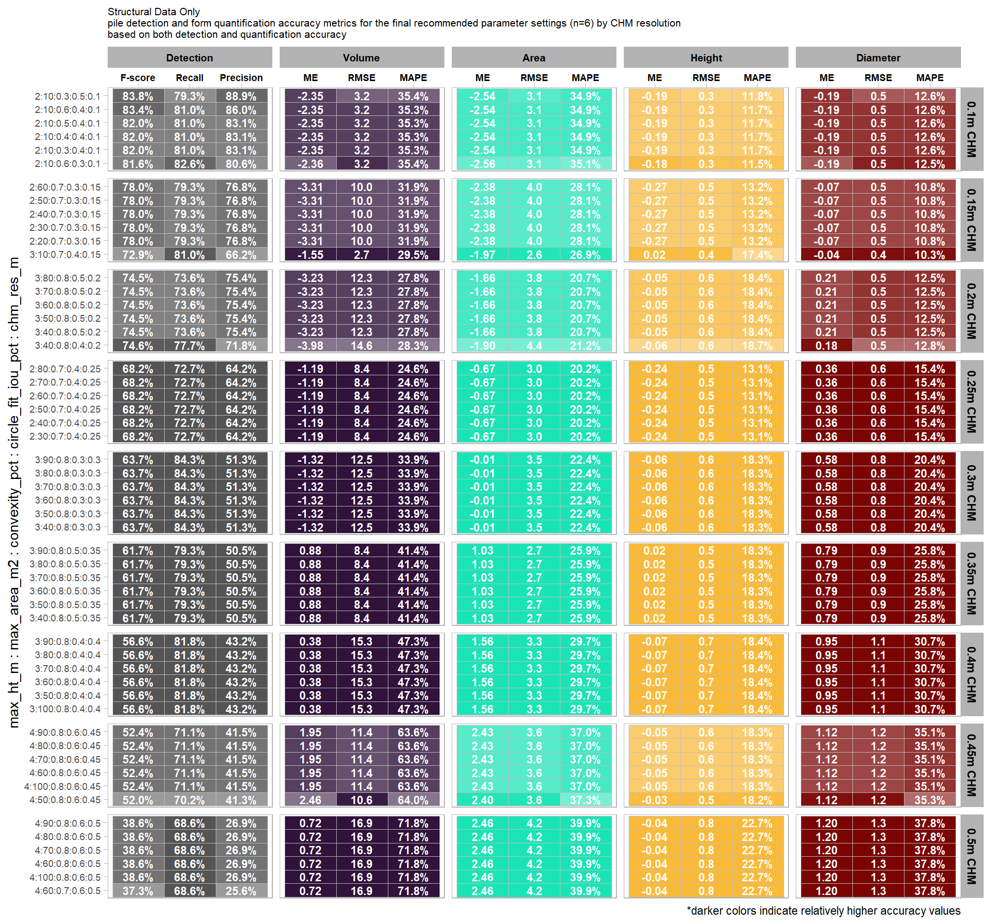
this plot allows for a simultaneous comparison of all metrics for pile detection and pile form quantification. it includes only the parameter combinations that achieved the best balanced accuracy, helping users identify the optimal settings by evaluating the trade-offs between detection and form quantification.
let’s table this
param_combos_ranked %>%
  dplyr::filter(is_final_selection_chm) %>%
  dplyr::select(!tidyselect::contains("_pct_rank_")) %>%
  # first select to arrange eval_metric
  dplyr::select(
    chm_lab, chm_res_m_desc
    , max_ht_m,max_area_m2,convexity_pct,circle_fit_iou_pct,chm_res_m
    # detection
    , f_score, recall, precision
    # quantification
    , tidyselect::ends_with("_mean")
    , tidyselect::ends_with("_rmse")
    # , tidyselect::ends_with("_rrmse")
    , tidyselect::ends_with("_mape")
  ) %>%
  # second select to arrange pile_metric
  dplyr::select(
    chm_lab, chm_res_m_desc
    , max_ht_m,max_area_m2,convexity_pct,circle_fit_iou_pct,chm_res_m
    # detection
    , f_score, recall, precision
    # quantification
    , c(tidyselect::contains("volume") & !tidyselect::contains("paraboloid"))
    , tidyselect::contains("area")
    , tidyselect::contains("height")
    , tidyselect::contains("diameter")
  ) %>%
  # names()
  dplyr::mutate(
    dplyr::across(
      .cols = c(f_score, recall, precision, tidyselect::ends_with("_mape"))
      , .fn = ~ scales::percent(.x, accuracy = 1)
    )
    , dplyr::across(
      .cols = c(tidyselect::ends_with("_mean"))
      , .fn = ~ scales::comma(.x, accuracy = 0.01)
    )
    , dplyr::across(
      .cols = c(tidyselect::ends_with("_rmse"))
      , .fn = ~ scales::comma(.x, accuracy = 0.1)
    )
  ) %>%
  dplyr::mutate(blank= "   " ) %>%
  dplyr::relocate(blank, .before = f_score) %>%
  dplyr::arrange(chm_res_m, desc(chm_lab)) %>%
  dplyr::select(-chm_res_m) %>%
  dplyr::relocate(chm_res_m_desc) %>%
  kableExtra::kbl(
    caption =
      paste0(
       "Structural Data Only"
       , "<br>pile detection and form quantification accuracy metrics for the final recommended parameter settings"
       # , scales::percent(1-pct_rank_th_top,accuracy=1)
       , " (n="
       , scales::comma(n_th_top_chm,accuracy=1)
       , ") by CHM resolution "
       , "<br>based on both detection and quantification accuracy"
      )
    , col.names = c(
      ".", ""
      ,"max_ht_m","max_area_m2","convexity_pct","circle_fit_iou_pct"
      , "   "
      , "F-score", "Recall", "Precision"
      , rep(c("ME","RMSE","MAPE"), times = 4)
    )
    , escape = F
  ) %>%
  kableExtra::kable_styling(font_size = 11) %>%
  kableExtra::add_header_above(c(
    " "=7
    , "Detection" = 3
    , "Volume" = 3
    , "Area" = 3
    , "Height" = 3
    , "Diameter" = 3
  )) %>%
  kableExtra::column_spec(seq(7,22,by=3), border_right = TRUE, include_thead = TRUE) %>%
  kableExtra::column_spec(
    column = 7:22
    , extra_css = "font-size: 10px;"
    , include_thead = T
  ) %>%
  kableExtra::collapse_rows(columns = 1, valign = "top") %>%
kableExtra::scroll_box(width = "740px") | . | max_ht_m | max_area_m2 | convexity_pct | circle_fit_iou_pct | F-score | Recall | Precision | ME | RMSE | MAPE | ME | RMSE | MAPE | ME | RMSE | MAPE | ME | RMSE | MAPE | ||
|---|---|---|---|---|---|---|---|---|---|---|---|---|---|---|---|---|---|---|---|---|---|
| 0.1m CHM | 2:10:0.3:0.5:0.1 | 2 | 10 | 0.3 | 0.5 | 84% | 79% | 89% | -2.35 | 3.2 | 35% | -2.54 | 3.1 | 35% | -0.19 | 0.3 | 12% | -0.19 | 0.5 | 13% | |
| 2:10:0.6:0.4:0.1 | 2 | 10 | 0.6 | 0.4 | 83% | 81% | 86% | -2.35 | 3.2 | 35% | -2.54 | 3.1 | 35% | -0.19 | 0.3 | 12% | -0.19 | 0.5 | 13% | ||
| 2:10:0.5:0.4:0.1 | 2 | 10 | 0.5 | 0.4 | 82% | 81% | 83% | -2.35 | 3.2 | 35% | -2.54 | 3.1 | 35% | -0.19 | 0.3 | 12% | -0.19 | 0.5 | 13% | ||
| 2:10:0.4:0.4:0.1 | 2 | 10 | 0.4 | 0.4 | 82% | 81% | 83% | -2.35 | 3.2 | 35% | -2.54 | 3.1 | 35% | -0.19 | 0.3 | 12% | -0.19 | 0.5 | 13% | ||
| 2:10:0.3:0.4:0.1 | 2 | 10 | 0.3 | 0.4 | 82% | 81% | 83% | -2.35 | 3.2 | 35% | -2.54 | 3.1 | 35% | -0.19 | 0.3 | 12% | -0.19 | 0.5 | 13% | ||
| 2:10:0.6:0.3:0.1 | 2 | 10 | 0.6 | 0.3 | 82% | 83% | 81% | -2.36 | 3.2 | 35% | -2.56 | 3.1 | 35% | -0.18 | 0.3 | 12% | -0.19 | 0.5 | 13% | ||
| 0.15m CHM | 2:60:0.7:0.3:0.15 | 2 | 60 | 0.7 | 0.3 | 78% | 79% | 77% | -3.31 | 10.0 | 32% | -2.38 | 4.0 | 28% | -0.27 | 0.5 | 13% | -0.07 | 0.5 | 11% | |
| 2:50:0.7:0.3:0.15 | 2 | 50 | 0.7 | 0.3 | 78% | 79% | 77% | -3.31 | 10.0 | 32% | -2.38 | 4.0 | 28% | -0.27 | 0.5 | 13% | -0.07 | 0.5 | 11% | ||
| 2:40:0.7:0.3:0.15 | 2 | 40 | 0.7 | 0.3 | 78% | 79% | 77% | -3.31 | 10.0 | 32% | -2.38 | 4.0 | 28% | -0.27 | 0.5 | 13% | -0.07 | 0.5 | 11% | ||
| 2:30:0.7:0.3:0.15 | 2 | 30 | 0.7 | 0.3 | 78% | 79% | 77% | -3.31 | 10.0 | 32% | -2.38 | 4.0 | 28% | -0.27 | 0.5 | 13% | -0.07 | 0.5 | 11% | ||
| 2:20:0.7:0.3:0.15 | 2 | 20 | 0.7 | 0.3 | 78% | 79% | 77% | -3.31 | 10.0 | 32% | -2.38 | 4.0 | 28% | -0.27 | 0.5 | 13% | -0.07 | 0.5 | 11% | ||
| 3:10:0.7:0.4:0.15 | 3 | 10 | 0.7 | 0.4 | 73% | 81% | 66% | -1.55 | 2.7 | 30% | -1.97 | 2.6 | 27% | 0.02 | 0.4 | 17% | -0.04 | 0.4 | 10% | ||
| 0.2m CHM | 3:80:0.8:0.5:0.2 | 3 | 80 | 0.8 | 0.5 | 74% | 74% | 75% | -3.23 | 12.3 | 28% | -1.66 | 3.8 | 21% | -0.05 | 0.6 | 18% | 0.21 | 0.5 | 13% | |
| 3:70:0.8:0.5:0.2 | 3 | 70 | 0.8 | 0.5 | 74% | 74% | 75% | -3.23 | 12.3 | 28% | -1.66 | 3.8 | 21% | -0.05 | 0.6 | 18% | 0.21 | 0.5 | 13% | ||
| 3:60:0.8:0.5:0.2 | 3 | 60 | 0.8 | 0.5 | 74% | 74% | 75% | -3.23 | 12.3 | 28% | -1.66 | 3.8 | 21% | -0.05 | 0.6 | 18% | 0.21 | 0.5 | 13% | ||
| 3:50:0.8:0.5:0.2 | 3 | 50 | 0.8 | 0.5 | 74% | 74% | 75% | -3.23 | 12.3 | 28% | -1.66 | 3.8 | 21% | -0.05 | 0.6 | 18% | 0.21 | 0.5 | 13% | ||
| 3:40:0.8:0.5:0.2 | 3 | 40 | 0.8 | 0.5 | 74% | 74% | 75% | -3.23 | 12.3 | 28% | -1.66 | 3.8 | 21% | -0.05 | 0.6 | 18% | 0.21 | 0.5 | 13% | ||
| 3:40:0.8:0.4:0.2 | 3 | 40 | 0.8 | 0.4 | 75% | 78% | 72% | -3.98 | 14.6 | 28% | -1.90 | 4.4 | 21% | -0.06 | 0.6 | 19% | 0.18 | 0.5 | 13% | ||
| 0.25m CHM | 2:80:0.7:0.4:0.25 | 2 | 80 | 0.7 | 0.4 | 68% | 73% | 64% | -1.19 | 8.4 | 25% | -0.67 | 3.0 | 20% | -0.24 | 0.5 | 13% | 0.36 | 0.6 | 15% | |
| 2:70:0.7:0.4:0.25 | 2 | 70 | 0.7 | 0.4 | 68% | 73% | 64% | -1.19 | 8.4 | 25% | -0.67 | 3.0 | 20% | -0.24 | 0.5 | 13% | 0.36 | 0.6 | 15% | ||
| 2:60:0.7:0.4:0.25 | 2 | 60 | 0.7 | 0.4 | 68% | 73% | 64% | -1.19 | 8.4 | 25% | -0.67 | 3.0 | 20% | -0.24 | 0.5 | 13% | 0.36 | 0.6 | 15% | ||
| 2:50:0.7:0.4:0.25 | 2 | 50 | 0.7 | 0.4 | 68% | 73% | 64% | -1.19 | 8.4 | 25% | -0.67 | 3.0 | 20% | -0.24 | 0.5 | 13% | 0.36 | 0.6 | 15% | ||
| 2:40:0.7:0.4:0.25 | 2 | 40 | 0.7 | 0.4 | 68% | 73% | 64% | -1.19 | 8.4 | 25% | -0.67 | 3.0 | 20% | -0.24 | 0.5 | 13% | 0.36 | 0.6 | 15% | ||
| 2:30:0.7:0.4:0.25 | 2 | 30 | 0.7 | 0.4 | 68% | 73% | 64% | -1.19 | 8.4 | 25% | -0.67 | 3.0 | 20% | -0.24 | 0.5 | 13% | 0.36 | 0.6 | 15% | ||
| 0.3m CHM | 3:90:0.8:0.3:0.3 | 3 | 90 | 0.8 | 0.3 | 64% | 84% | 51% | -1.32 | 12.5 | 34% | -0.01 | 3.5 | 22% | -0.06 | 0.6 | 18% | 0.58 | 0.8 | 20% | |
| 3:80:0.8:0.3:0.3 | 3 | 80 | 0.8 | 0.3 | 64% | 84% | 51% | -1.32 | 12.5 | 34% | -0.01 | 3.5 | 22% | -0.06 | 0.6 | 18% | 0.58 | 0.8 | 20% | ||
| 3:70:0.8:0.3:0.3 | 3 | 70 | 0.8 | 0.3 | 64% | 84% | 51% | -1.32 | 12.5 | 34% | -0.01 | 3.5 | 22% | -0.06 | 0.6 | 18% | 0.58 | 0.8 | 20% | ||
| 3:60:0.8:0.3:0.3 | 3 | 60 | 0.8 | 0.3 | 64% | 84% | 51% | -1.32 | 12.5 | 34% | -0.01 | 3.5 | 22% | -0.06 | 0.6 | 18% | 0.58 | 0.8 | 20% | ||
| 3:50:0.8:0.3:0.3 | 3 | 50 | 0.8 | 0.3 | 64% | 84% | 51% | -1.32 | 12.5 | 34% | -0.01 | 3.5 | 22% | -0.06 | 0.6 | 18% | 0.58 | 0.8 | 20% | ||
| 3:40:0.8:0.3:0.3 | 3 | 40 | 0.8 | 0.3 | 64% | 84% | 51% | -1.32 | 12.5 | 34% | -0.01 | 3.5 | 22% | -0.06 | 0.6 | 18% | 0.58 | 0.8 | 20% | ||
| 0.35m CHM | 3:90:0.8:0.5:0.35 | 3 | 90 | 0.8 | 0.5 | 62% | 79% | 51% | 0.88 | 8.4 | 41% | 1.03 | 2.7 | 26% | 0.02 | 0.5 | 18% | 0.79 | 0.9 | 26% | |
| 3:80:0.8:0.5:0.35 | 3 | 80 | 0.8 | 0.5 | 62% | 79% | 51% | 0.88 | 8.4 | 41% | 1.03 | 2.7 | 26% | 0.02 | 0.5 | 18% | 0.79 | 0.9 | 26% | ||
| 3:70:0.8:0.5:0.35 | 3 | 70 | 0.8 | 0.5 | 62% | 79% | 51% | 0.88 | 8.4 | 41% | 1.03 | 2.7 | 26% | 0.02 | 0.5 | 18% | 0.79 | 0.9 | 26% | ||
| 3:60:0.8:0.5:0.35 | 3 | 60 | 0.8 | 0.5 | 62% | 79% | 51% | 0.88 | 8.4 | 41% | 1.03 | 2.7 | 26% | 0.02 | 0.5 | 18% | 0.79 | 0.9 | 26% | ||
| 3:50:0.8:0.5:0.35 | 3 | 50 | 0.8 | 0.5 | 62% | 79% | 51% | 0.88 | 8.4 | 41% | 1.03 | 2.7 | 26% | 0.02 | 0.5 | 18% | 0.79 | 0.9 | 26% | ||
| 3:40:0.8:0.5:0.35 | 3 | 40 | 0.8 | 0.5 | 62% | 79% | 51% | 0.88 | 8.4 | 41% | 1.03 | 2.7 | 26% | 0.02 | 0.5 | 18% | 0.79 | 0.9 | 26% | ||
| 0.4m CHM | 3:90:0.8:0.4:0.4 | 3 | 90 | 0.8 | 0.4 | 57% | 82% | 43% | 0.38 | 15.3 | 47% | 1.56 | 3.3 | 30% | -0.07 | 0.7 | 18% | 0.95 | 1.1 | 31% | |
| 3:80:0.8:0.4:0.4 | 3 | 80 | 0.8 | 0.4 | 57% | 82% | 43% | 0.38 | 15.3 | 47% | 1.56 | 3.3 | 30% | -0.07 | 0.7 | 18% | 0.95 | 1.1 | 31% | ||
| 3:70:0.8:0.4:0.4 | 3 | 70 | 0.8 | 0.4 | 57% | 82% | 43% | 0.38 | 15.3 | 47% | 1.56 | 3.3 | 30% | -0.07 | 0.7 | 18% | 0.95 | 1.1 | 31% | ||
| 3:60:0.8:0.4:0.4 | 3 | 60 | 0.8 | 0.4 | 57% | 82% | 43% | 0.38 | 15.3 | 47% | 1.56 | 3.3 | 30% | -0.07 | 0.7 | 18% | 0.95 | 1.1 | 31% | ||
| 3:50:0.8:0.4:0.4 | 3 | 50 | 0.8 | 0.4 | 57% | 82% | 43% | 0.38 | 15.3 | 47% | 1.56 | 3.3 | 30% | -0.07 | 0.7 | 18% | 0.95 | 1.1 | 31% | ||
| 3:100:0.8:0.4:0.4 | 3 | 100 | 0.8 | 0.4 | 57% | 82% | 43% | 0.38 | 15.3 | 47% | 1.56 | 3.3 | 30% | -0.07 | 0.7 | 18% | 0.95 | 1.1 | 31% | ||
| 0.45m CHM | 4:90:0.8:0.6:0.45 | 4 | 90 | 0.8 | 0.6 | 52% | 71% | 42% | 1.95 | 11.4 | 64% | 2.43 | 3.6 | 37% | -0.05 | 0.6 | 18% | 1.12 | 1.2 | 35% | |
| 4:80:0.8:0.6:0.45 | 4 | 80 | 0.8 | 0.6 | 52% | 71% | 42% | 1.95 | 11.4 | 64% | 2.43 | 3.6 | 37% | -0.05 | 0.6 | 18% | 1.12 | 1.2 | 35% | ||
| 4:70:0.8:0.6:0.45 | 4 | 70 | 0.8 | 0.6 | 52% | 71% | 42% | 1.95 | 11.4 | 64% | 2.43 | 3.6 | 37% | -0.05 | 0.6 | 18% | 1.12 | 1.2 | 35% | ||
| 4:60:0.8:0.6:0.45 | 4 | 60 | 0.8 | 0.6 | 52% | 71% | 42% | 1.95 | 11.4 | 64% | 2.43 | 3.6 | 37% | -0.05 | 0.6 | 18% | 1.12 | 1.2 | 35% | ||
| 4:100:0.8:0.6:0.45 | 4 | 100 | 0.8 | 0.6 | 52% | 71% | 42% | 1.95 | 11.4 | 64% | 2.43 | 3.6 | 37% | -0.05 | 0.6 | 18% | 1.12 | 1.2 | 35% | ||
| 4:50:0.8:0.6:0.45 | 4 | 50 | 0.8 | 0.6 | 52% | 70% | 41% | 2.46 | 10.6 | 64% | 2.40 | 3.6 | 37% | -0.03 | 0.5 | 18% | 1.12 | 1.2 | 35% | ||
| 0.5m CHM | 4:90:0.8:0.6:0.5 | 4 | 90 | 0.8 | 0.6 | 39% | 69% | 27% | 0.72 | 16.9 | 72% | 2.46 | 4.2 | 40% | -0.04 | 0.8 | 23% | 1.20 | 1.3 | 38% | |
| 4:80:0.8:0.6:0.5 | 4 | 80 | 0.8 | 0.6 | 39% | 69% | 27% | 0.72 | 16.9 | 72% | 2.46 | 4.2 | 40% | -0.04 | 0.8 | 23% | 1.20 | 1.3 | 38% | ||
| 4:70:0.8:0.6:0.5 | 4 | 70 | 0.8 | 0.6 | 39% | 69% | 27% | 0.72 | 16.9 | 72% | 2.46 | 4.2 | 40% | -0.04 | 0.8 | 23% | 1.20 | 1.3 | 38% | ||
| 4:60:0.8:0.6:0.5 | 4 | 60 | 0.8 | 0.6 | 39% | 69% | 27% | 0.72 | 16.9 | 72% | 2.46 | 4.2 | 40% | -0.04 | 0.8 | 23% | 1.20 | 1.3 | 38% | ||
| 4:100:0.8:0.6:0.5 | 4 | 100 | 0.8 | 0.6 | 39% | 69% | 27% | 0.72 | 16.9 | 72% | 2.46 | 4.2 | 40% | -0.04 | 0.8 | 23% | 1.20 | 1.3 | 38% | ||
| 4:60:0.7:0.6:0.5 | 4 | 60 | 0.7 | 0.6 | 37% | 69% | 26% | 0.72 | 16.9 | 72% | 2.46 | 4.2 | 40% | -0.04 | 0.8 | 23% | 1.20 | 1.3 | 38% |
what is the expected detection accuracy of the final 6 recommended settings by CHM resolution?
plt_detection_dist2(
  df = param_combos_ranked %>% dplyr::filter(is_final_selection_chm) %>% dplyr::select(!tidyselect::contains("_pct_rank_"))
  , paste0(
    "Structural Data Only"
    , "\ndistribution of evaluation metrics for the final recommended parameter settings"
    , " (n="
    , scales::comma(n_th_top_chm,accuracy=1)
    , ") by CHM resolution"
    , "\nbased on both detection and quantification accuracy"
  )
)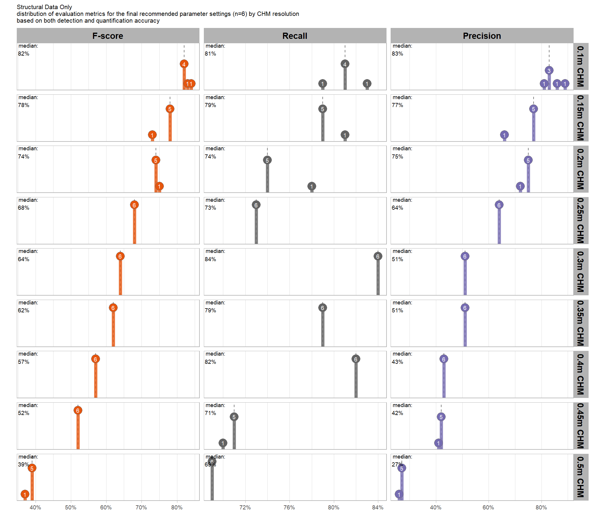
WHAT DID WE LEARN FROM THIS
what is the expected MAPE of the final 6 recommended settings by CHM resolution?
# plot it
plt_form_quantification_dist2(
  df = param_combos_ranked %>% dplyr::filter(is_final_selection_chm) %>% dplyr::select(!tidyselect::contains("_pct_rank_"))
  , quant_metric = "mape"
  , paste0(
    "Structural Data Only"
    , "\ndistribution of pile form quantification metrics for the final recommended parameter settings"
    , " (n="
    , scales::comma(n_th_top_chm,accuracy=1)
    , ") by CHM resolution"
    , "\nbased on both detection and quantification accuracy"
  )
)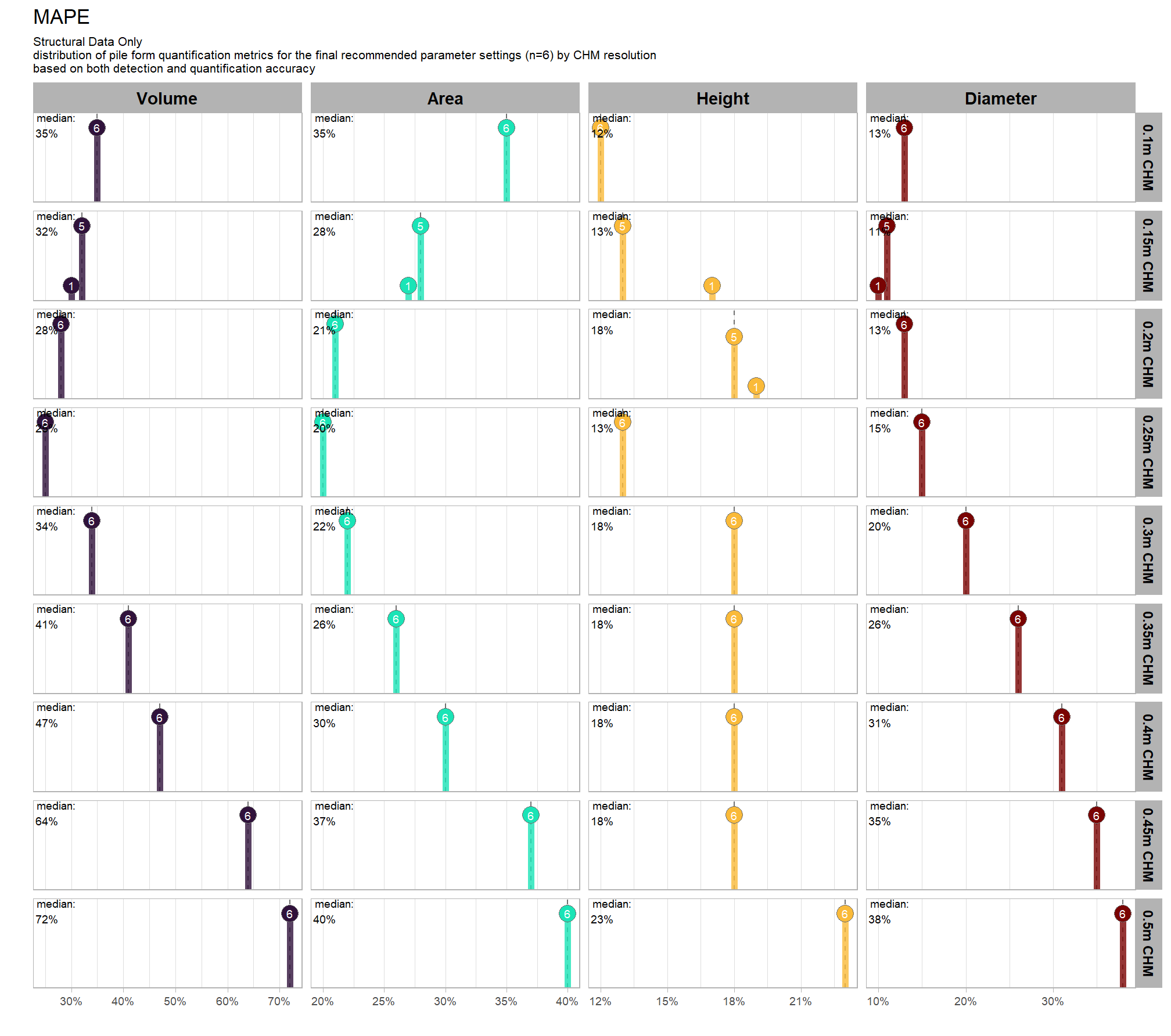
WHAT DID WE LEARN FROM THIS
what is the expected Mean Error (ME) of the final 6 recommended settings by CHM resolution?
# plot it
plt_form_quantification_dist2(
  df = param_combos_ranked %>% dplyr::filter(is_final_selection_chm) %>% dplyr::select(!tidyselect::contains("_pct_rank_"))
  , quant_metric = "mean"
  , paste0(
    "Structural Data Only"
    , "\ndistribution of pile form quantification metrics for the final recommended parameter settings"
    , " (n="
    , scales::comma(n_th_top_chm,accuracy=1)
    , ") by CHM resolution"
    , "\nbased on both detection and quantification accuracy"
  )
)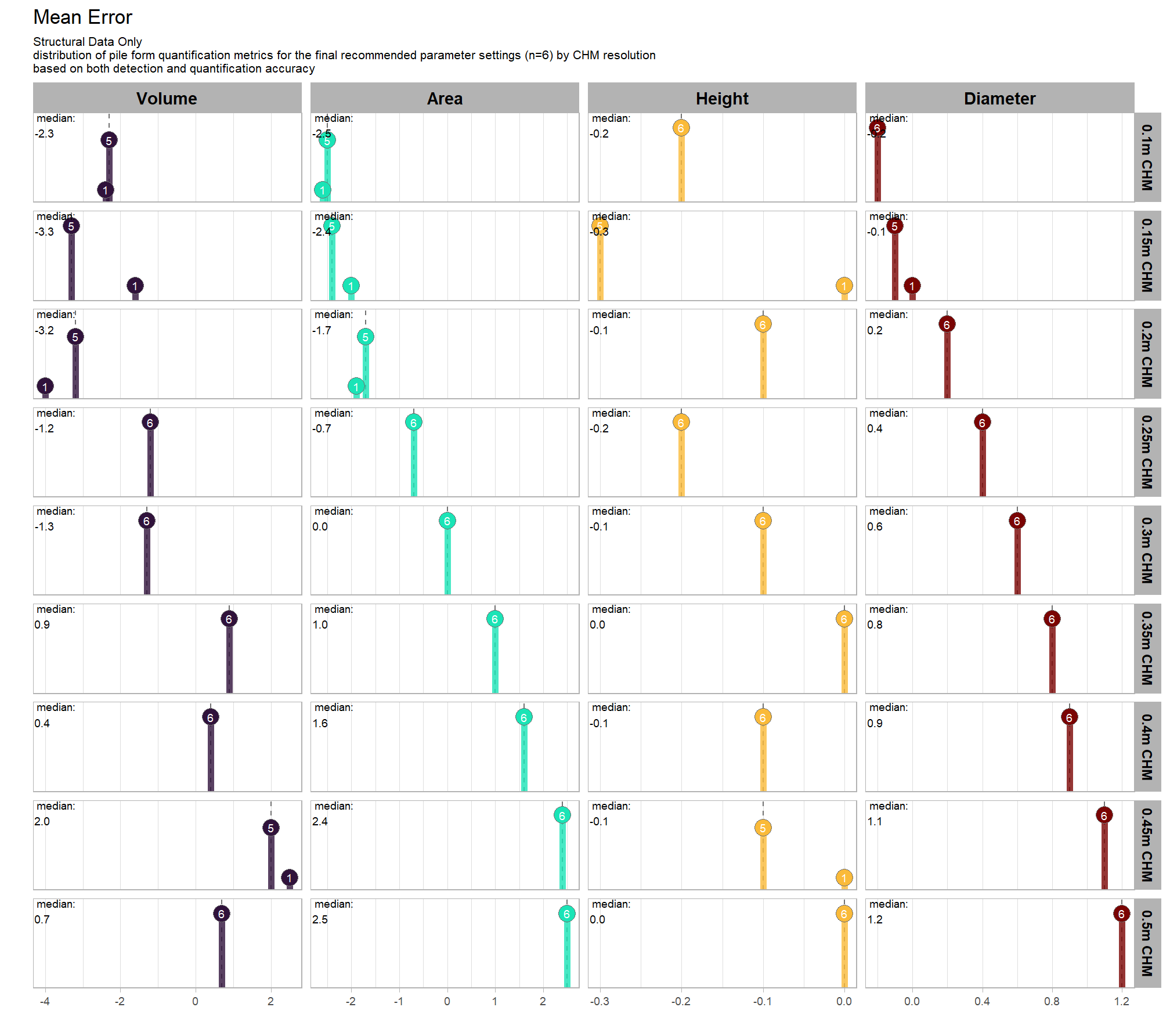
WHAT DID WE LEARN FROM THIS
what is the expected RMSE of the final 6 recommended settings by CHM resolution?
# plot it
plt_form_quantification_dist2(
  df = param_combos_ranked %>% dplyr::filter(is_final_selection_chm) %>% dplyr::select(!tidyselect::contains("_pct_rank_"))
  , quant_metric = "rmse"
  , paste0(
    "Structural Data Only"
    , "\ndistribution of pile form quantification metrics for the final recommended parameter settings"
    , " (n="
    , scales::comma(n_th_top_chm,accuracy=1)
    , ") by CHM resolution"
    , "\nbased on both detection and quantification accuracy"
  )
)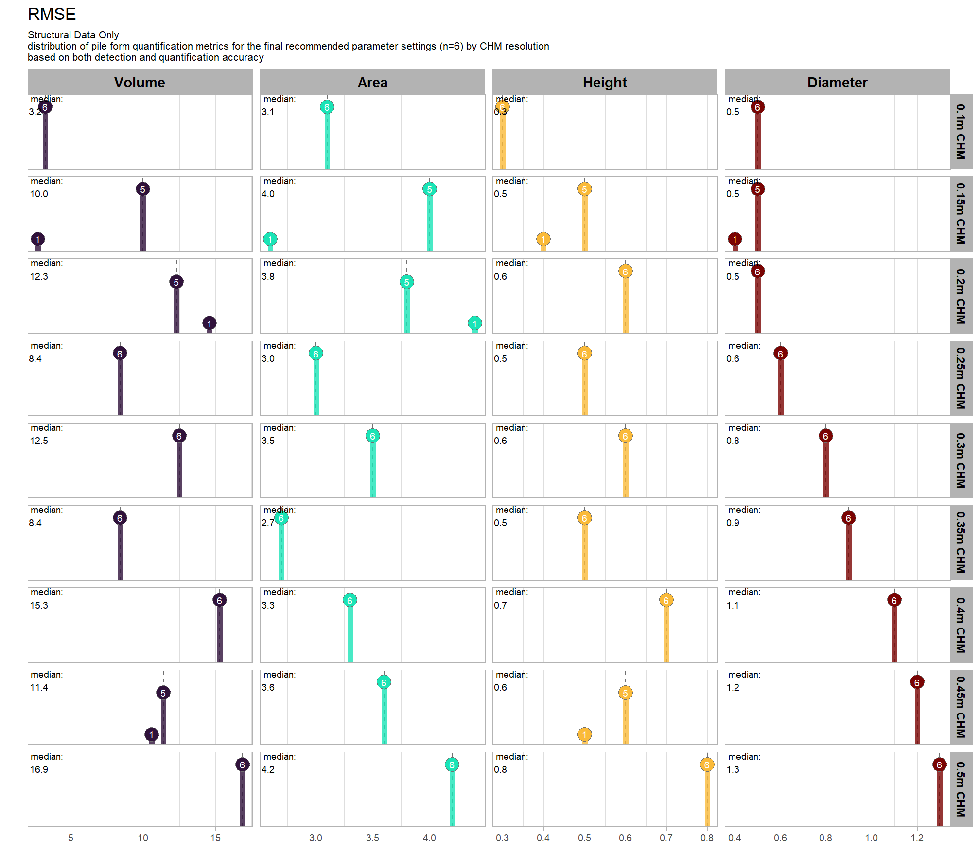
WHAT DID WE LEARN FROM THIS
9.6 Data Fusion: Sensitivity Testing
let’s look at the sensitivity testing results for the data fusion approach approach that uses both a CHM generated from aerial point cloud data (for structural information) and RGB imagery
we tested a total of 8,640 combinations tested per CHM resolution and an overall total of 77,760 combinations tested
9.6.1 Main Effects: pile detection
what is the detection accuracy across all parameter combinations tested for each CHM resolution?
# plot it
plt_detection_dist2(
  df = param_combos_spectral_gt_agg
  , paste0(
     "Data Fusion"
      , "\ndistribution of pile detection accuracy metrics for all"
     , " (n="
     , scales::comma(n_combos_tested_spectral_chm, accuracy = 1)
     , ") "
     , "parameter combinations tested by CHM resolution"
    )
  , show_rug = F
)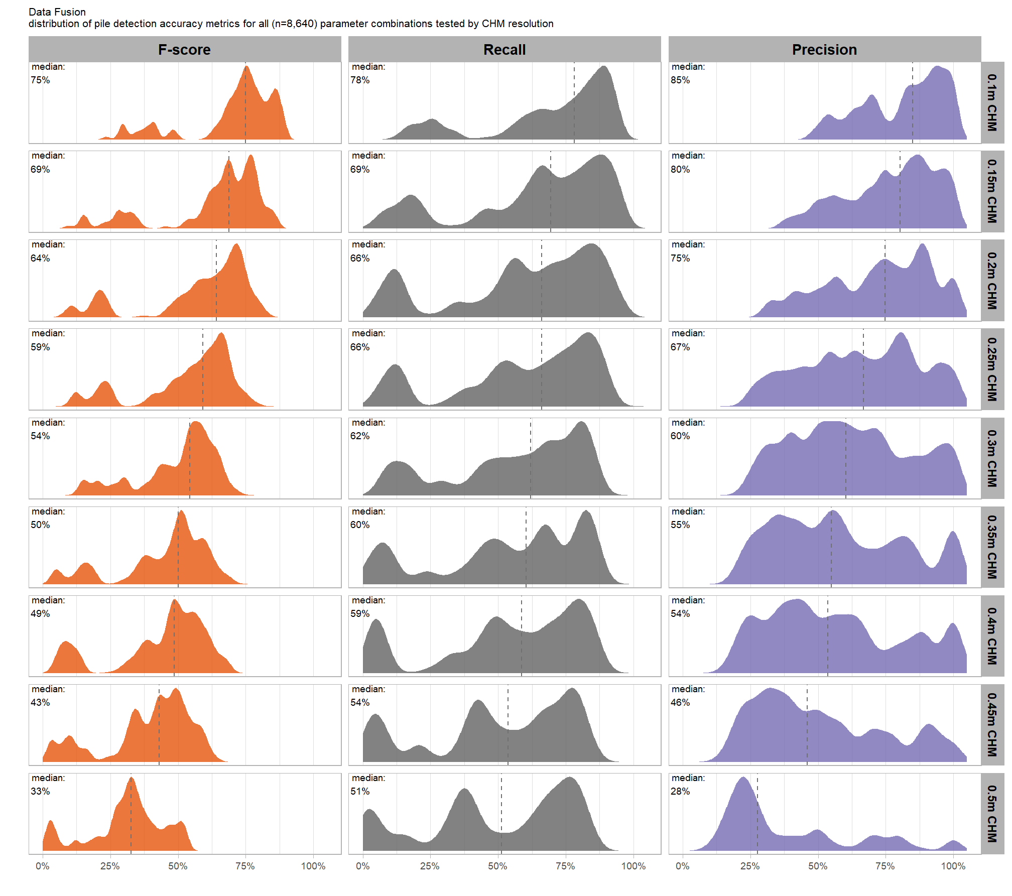
collapsing across all other parameters, what is the main effect of each individual parameter, including the spectral_weight parameter from the data fusion approach, or CHM resolution?
param_combos_spectral_gt_agg %>%
  tidyr::pivot_longer(
    cols = c(precision,recall,f_score)
    , names_to = "metric"
    , values_to = "value"
  ) %>%
  tidyr::pivot_longer(
    cols = c(max_ht_m,max_area_m2,convexity_pct,circle_fit_iou_pct,chm_res_m,spectral_weight)
    , names_to = "param"
    , values_to = "param_value"
  ) %>%
  dplyr::group_by(param, param_value, metric) %>%
  dplyr::summarise(
    median = median(value,na.rm=T)
    , q25 = stats::quantile(value,na.rm=T,probs = 0.25)
    , q75 = stats::quantile(value,na.rm=T,probs = 0.75)
  ) %>%
  dplyr::ungroup() %>%
  dplyr::mutate(
    param = dplyr::case_when(
        param == "spectral_weight" ~ 1
        , param == "chm_res_m" ~ 2
        , param == "max_ht_m" ~ 3
        , param == "min_area_m2" ~ 4
        , param == "max_area_m2" ~ 5
        , param == "convexity_pct" ~ 6
        , param == "circle_fit_iou_pct" ~ 7
      ) %>%
      factor(
        ordered = T
        , levels = 1:7
        , labels = c(
          "spectral_weight"
          , "CHM resolution (m)"
          , "max_ht_m"
          , "min_area_m2"
          , "max_area_m2"
          , "convexity_pct"
          , "circle_fit_iou_pct"
        )
      )
    , metric = dplyr::case_when(
        metric == "f_score" ~ 1
        , metric == "recall" ~ 2
        , metric == "precision" ~ 3
      ) %>%
      factor(
        ordered = T
        , levels = 1:3
        , labels = c(
          "F-score"
          , "Recall"
          , "Precision"
        )
      ) %>%
      forcats::fct_rev()
  ) %>%
  ggplot2::ggplot(
    mapping = ggplot2::aes(y = median, x = param_value, color = metric, fill = metric, group = metric, shape = metric)
  ) +
  ggplot2::geom_ribbon(
    mapping = ggplot2::aes(ymin = q25, ymax = q75)
    , alpha = 0.2, color = NA
  ) +
  ggplot2::geom_line(lwd = 1.5, alpha = 0.8) +
  ggplot2::geom_point(size = 2) +
  ggplot2::facet_wrap(facets = dplyr::vars(param), scales = "free_x") +
  # ggplot2::scale_color_viridis_d(begin = 0.2, end = 0.8) +
  ggplot2::scale_fill_manual(values = rev(pal_eval_metric)) +
  ggplot2::scale_color_manual(values = rev(pal_eval_metric)) +
  ggplot2::scale_y_continuous(limits = c(0,1), labels = scales::percent, breaks = scales::breaks_extended(10)) +
  ggplot2::labs(x = "", y = "median value", color = "", fill = "") +
  ggplot2::theme_light() +
  ggplot2::theme(
    legend.position = "top"
    , strip.text = ggplot2::element_text(size = 11, color = "black", face = "bold")
  ) +
  ggplot2::guides(
    color = ggplot2::guide_legend(override.aes = list(shape = 15, linetype = 0, size = 5, alpha = 1))
    , shape = "none"
  )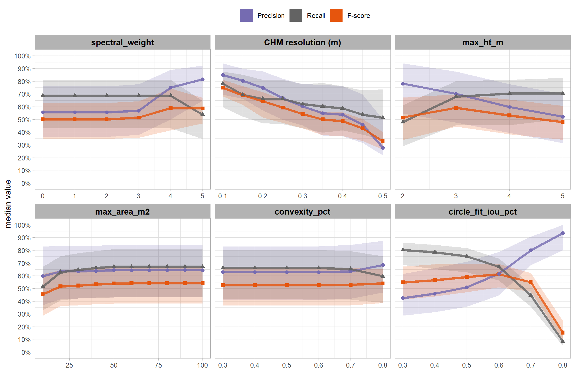
based on these main effect aggregated results, the influence of the parameters specific to the structural detection of slash piles remained the same as when tested without the spectral data. with respect to the spectral_weight parameter included in the data fusion approach:
- increasing the
spectral_weight(where “5” requires all spectral index thresholds to be met) had minimal impact on metrics until a value of “3”, at which point F-score and precision both saw slight improvements. at aspectral_weightof “4”, the F-score significantly improved due to a substantial increase in precision. settingspectral_weightto “5” resulted in a significant drop in recall (detection rate) and a proportionally inverse increase in precision, leading to only a minor overall change in F-score.
9.6.2 Main Effects: form quantification
let’s check out the the ability of the method to properly extract the form of the piles by looking at the quantification accuracy metrics where:
- Mean Error (ME) represents the direction of bias (over or under-prediction) in the original units
- RMSE represents the typical magnitude of error in the original units, with a stronger penalty for large errors
- MAPE represents the typical magnitude of error as a percentage, allowing for scale-independent comparisons
we expect that the spectral data does not alter the quantification of slash pile form. this is because spectral information is used solely to filter candidate piles, meaning it neither reshapes existing ones nor introduces new detections.
let’s average across all other factors to look at the main effect by parameter for the MAPE metrics quantifying the pile form accuracy
param_combos_spectral_gt_agg %>%
  dplyr::select(
    spectral_weight
    , tidyselect::ends_with("_mape")
  ) %>%
  tidyr::pivot_longer(
    cols = c(tidyselect::ends_with("_mape"))
    , names_to = "metric"
    , values_to = "value"
  ) %>%
  tidyr::pivot_longer(
    cols = c(spectral_weight)
    , names_to = "param"
    , values_to = "param_value"
  ) %>%
  dplyr::group_by(param, param_value, metric) %>%
  dplyr::summarise(
    median = median(value,na.rm=T)
    , q25 = stats::quantile(value,na.rm=T,probs = 0.25)
    , q75 = stats::quantile(value,na.rm=T,probs = 0.75)
  ) %>%
  dplyr::ungroup() %>%
  dplyr::mutate(
    metric = dplyr::case_when(
        metric == "f_score" ~ 1
        , metric == "recall" ~ 2
        , metric == "precision" ~ 3
        # rmse
        , metric == "pct_diff_volume_field_mape" ~ 4
        , metric == "pct_diff_paraboloid_volume_field_mape" ~ 5
        , metric == "pct_diff_area_field_mape" ~ 6
        , metric == "pct_diff_height_mape" ~ 7
        , metric == "pct_diff_diameter_mape" ~ 8
      ) %>%
      factor(
        ordered = T
        , levels = 1:8
        , labels = c(
          "F-score"
          , "Recall"
          , "Precision"
          , "MAPE: Volume irregular (%)"
          , "MAPE: Volume paraboloid (%)"
          , "MAPE: Area (%)"
          , "MAPE: Height (%)"
          , "MAPE: Diameter (%)"
        )
      )
    # , param_value = factor(x = param_value, labels = levels(param_combos_spectral_gt$spectral_weight_desc))
  ) %>%
  ggplot2::ggplot(
    mapping = ggplot2::aes(y = median, x = param_value, color = metric, fill = metric, group = metric, shape = metric)
  ) +
  # ggplot2::geom_ribbon(
  #   mapping = ggplot2::aes(ymin = q25, ymax = q75)
  #   , alpha = 0.2, color = NA
  # ) +
  ggplot2::geom_line(lwd = 1.5, alpha = 0.8) +
  ggplot2::geom_point(size = 2) +
  ggplot2::facet_wrap(facets = dplyr::vars(param), scales = "free_x") +
  ggplot2::scale_fill_viridis_d(option = "turbo") +
  ggplot2::scale_color_viridis_d(option = "turbo") +
  ggplot2::scale_shape_manual(values = c(15,16,17,18,0)) +
  ggplot2::scale_y_continuous(limits = c(0,1), labels = scales::percent, breaks = scales::breaks_extended(10)) +
  ggplot2::labs(x = "", y = "median value", color = "", fill = "") +
  ggplot2::theme_light() +
  ggplot2::theme(
    legend.position = "top"
    , strip.text = ggplot2::element_text(size = 11, color = "black", face = "bold")
  ) +
  ggplot2::guides(
    color = ggplot2::guide_legend(override.aes = list(shape = 15, linetype = 0, size = 5, alpha = 1))
    , shape = "none"
  )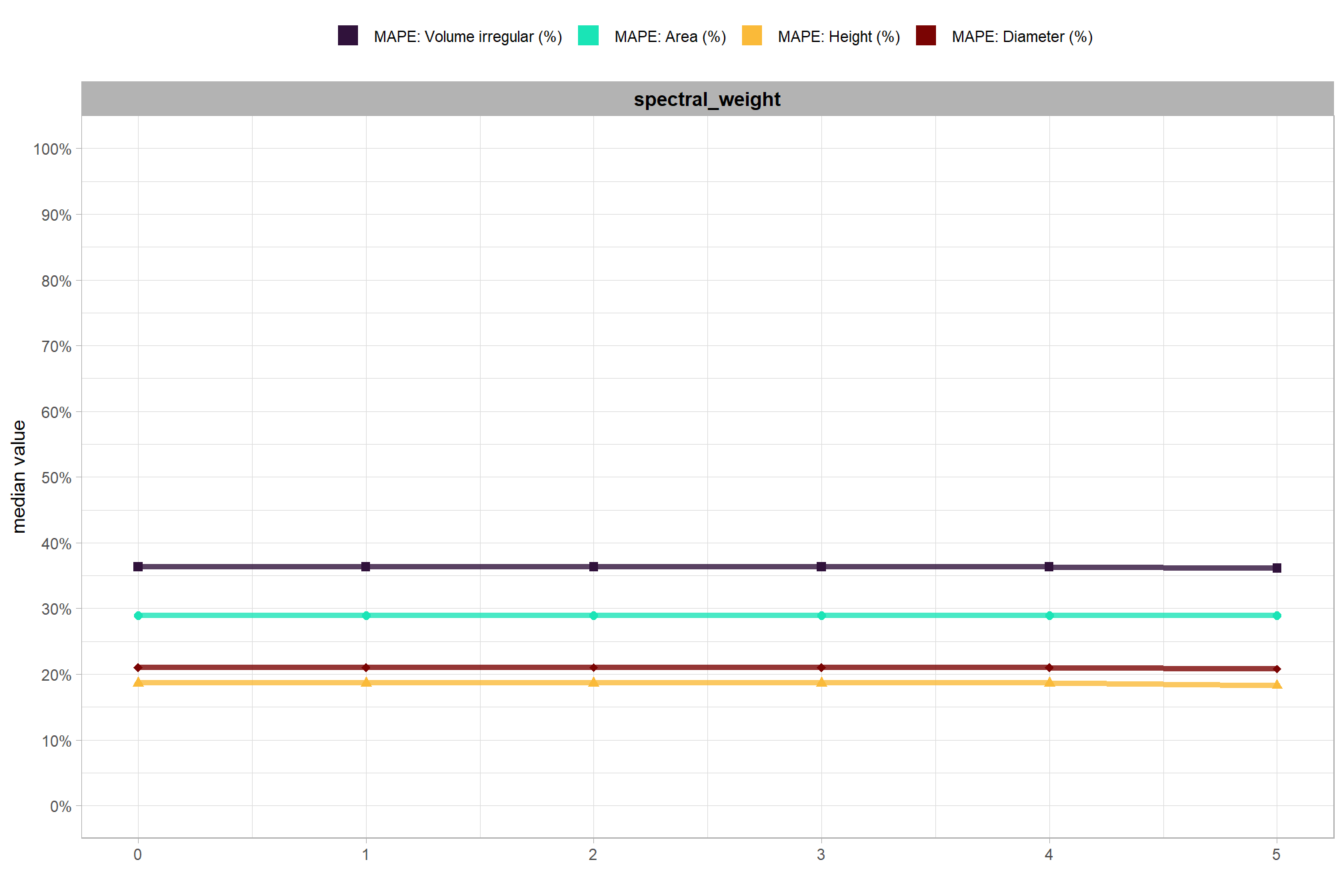
WHAT DID WE LEARN FROM THIS
9.6.3 Final recommended settings
let’s identify the best-performing parameter combinations that not only balance detection and quantification accuracy but also achieve the highest recall rates. we’ll select these by choosing any combination whose recall rate is at least one standard deviation above the average for this top group. if no combinations meet this criterion, we will instead select the top 10 combinations based on their recall rates.
9.6.3.1 Overall (across CHM resolution)
To select the best-performing parameter combinations, we will prioritize those that balance detection and quantification accuracy. From this group, we will then identify the settings that achieve the highest pile detection rates (recall). We emphasize that these recommendations are for users who can generate a CHM from the original point cloud. This is critical because creating a new CHM at the desired resolution is a fundamentally different process than simply disaggregating an existing, coarser raster.
we’ll use the F-Score and the average rank of the MAPE metrics across all form measurements (i.e. height, diameter, area, volume) to determine the best overall list
# param_combos_gt_agg %>% nrow()
param_combos_spectral_ranked <-
  param_combos_spectral_gt_agg %>%
  ##########
  # first. find overall top combinations irrespective of CHM res
  ##########
  dplyr::ungroup() %>%
  dplyr::mutate(
    # label combining params
    lab = stringr::str_c(max_ht_m,max_area_m2,convexity_pct,circle_fit_iou_pct,chm_res_m,spectral_weight, sep = ":")
    , dplyr::across(
      .cols = c(tidyselect::ends_with("_mape"))
      , .fn = ~dplyr::percent_rank(-.x)
      , .names = "ovrall_pct_rank_quant_{.col}"
    )
    , dplyr::across(
      .cols = c(f_score)
      # .cols = c(f_score,recall)
      , .fn = ~dplyr::percent_rank(.x)
      , .names = "ovrall_pct_rank_det_{.col}"
    )
  ) %>%
  ##########
  # second. find top combinations by CHM res
  ##########
  dplyr::group_by(chm_res_m) %>%
  dplyr::mutate(
    dplyr::across(
      .cols = c(tidyselect::ends_with("_mape") & !tidyselect::starts_with("ovrall_pct_rank_"))
      , .fn = ~dplyr::percent_rank(-.x)
      , .names = "chm_pct_rank_quant_{.col}"
    )
    , dplyr::across(
      .cols = c(f_score)
      # .cols = c(f_score,recall)
      , .fn = ~dplyr::percent_rank(.x)
      , .names = "chm_pct_rank_det_{.col}"
    )
  ) %>%
  # now get the max of these pct ranks by row
  dplyr::rowwise() %>%
  dplyr::mutate(
    ovrall_pct_rank_quant_mean = mean(
      dplyr::c_across(
        tidyselect::starts_with("ovrall_pct_rank_quant_")
      )
      , na.rm = T
    )
    , ovrall_pct_rank_det_mean = mean(
      dplyr::c_across(
        tidyselect::starts_with("ovrall_pct_rank_det_")
      )
      , na.rm = T
    )
    , chm_pct_rank_quant_mean = mean(
      dplyr::c_across(
        tidyselect::starts_with("chm_pct_rank_quant_")
      )
      , na.rm = T
    )
    , chm_pct_rank_det_mean = mean(
      dplyr::c_across(
        tidyselect::starts_with("chm_pct_rank_det_")
      )
      , na.rm = T
    )
  ) %>%
  dplyr::ungroup() %>%
  # now make quadrant var
  dplyr::mutate(
    # groupings for the quadrant plot
    ovrall_accuracy_grp = dplyr::case_when(
        ovrall_pct_rank_det_mean>=0.95 & ovrall_pct_rank_quant_mean>=0.95 ~ 1
        , ovrall_pct_rank_det_mean>=0.90 & ovrall_pct_rank_quant_mean>=0.90 ~ 2
        , ovrall_pct_rank_det_mean>=0.75 & ovrall_pct_rank_quant_mean>=0.75 ~ 3
        , ovrall_pct_rank_det_mean>=0.50 & ovrall_pct_rank_quant_mean>=0.50 ~ 4
        , ovrall_pct_rank_det_mean>=0.50 & ovrall_pct_rank_quant_mean<0.50 ~ 5
        , ovrall_pct_rank_det_mean<0.50 & ovrall_pct_rank_quant_mean>=0.50 ~ 6
        , T ~ 7
      ) %>%
      factor(
        ordered = T
        , levels = 1:7
        , labels = c(
          "top 5% detection & quantification" # ovrall_pct_rank_mean>=0.95 & ovrall_pct_rank_f_score>=0.95 ~ 1
          , "top 10% detection & quantification" # ovrall_pct_rank_mean>=0.90 & ovrall_pct_rank_f_score>=0.90 ~ 2
          , "top 25% detection & quantification" # ovrall_pct_rank_mean>=0.75 & ovrall_pct_rank_f_score>=0.75 ~ 3
          , "top 50% detection & quantification" # ovrall_pct_rank_mean>=0.50 & ovrall_pct_rank_f_score>=0.50 ~ 4
          , "top 50% quantification" # ovrall_pct_rank_mean>=0.50 & ovrall_pct_rank_f_score<0.50 ~ 5
          , "top 50% detection" # ovrall_pct_rank_mean<0.50 & ovrall_pct_rank_f_score>=0.50 ~ 6
          , "bottom 50% detection & quantification"
        )
      )
    , chm_accuracy_grp = dplyr::case_when(
        chm_pct_rank_det_mean>=0.95 & chm_pct_rank_quant_mean>=0.95 ~ 1
        , chm_pct_rank_det_mean>=0.90 & chm_pct_rank_quant_mean>=0.90 ~ 2
        , chm_pct_rank_det_mean>=0.75 & chm_pct_rank_quant_mean>=0.75 ~ 3
        , chm_pct_rank_det_mean>=0.50 & chm_pct_rank_quant_mean>=0.50 ~ 4
        , chm_pct_rank_det_mean>=0.50 & chm_pct_rank_quant_mean<0.50 ~ 5
        , chm_pct_rank_det_mean<0.50 & chm_pct_rank_quant_mean>=0.50 ~ 6
        , T ~ 7
      ) %>%
      factor(
        ordered = T
        , levels = 1:7
        , labels = c(
          "top 5% detection & quantification" # chm_pct_rank_mean>=0.95 & chm_pct_rank_f_score>=0.95 ~ 1
          , "top 10% detection & quantification" # chm_pct_rank_mean>=0.90 & chm_pct_rank_f_score>=0.90 ~ 2
          , "top 25% detection & quantification" # chm_pct_rank_mean>=0.75 & chm_pct_rank_f_score>=0.75 ~ 3
          , "top 50% detection & quantification" # chm_pct_rank_mean>=0.50 & chm_pct_rank_f_score>=0.50 ~ 4
          , "top 50% quantification" # chm_pct_rank_mean>=0.50 & chm_pct_rank_f_score<0.50 ~ 5
          , "top 50% detection" # chm_pct_rank_mean<0.50 & chm_pct_rank_f_score>=0.50 ~ 6
          , "bottom 50% detection & quantification"
        )
      )
    ,
  ) %>%
  ##########
  # first. find overall top combinations irrespective of CHM res
  ##########
  dplyr::ungroup() %>%
  dplyr::mutate(
    ovrall_balanced_pct_rank = dplyr::percent_rank( (ovrall_pct_rank_det_mean+ovrall_pct_rank_quant_mean)/2 ) # equally weight quant and detection
    , ovrall_lab = forcats::fct_reorder(lab, ovrall_balanced_pct_rank)
  ) %>%
  dplyr::arrange(desc(ovrall_balanced_pct_rank),desc(ovrall_pct_rank_det_mean),desc(ovrall_pct_rank_quant_mean)) %>%
  dplyr::mutate(
    ovrall_balanced_rank = dplyr::row_number()
    # is_top_overall = using rows in case not all combos resulted in piles and/or
      # there are many ties in the data leading to no records with a percent rank <= pct_th_top (e.g. many tied at 98%)
    , is_top_overall = dplyr::row_number()<=(n_combos_tested_spectral*pct_th_top)
      # ovrall_balanced_pct_rank>=(1-pct_th_top)
  ) %>%
  dplyr::arrange(desc(is_top_overall),desc(recall),desc(ovrall_pct_rank_det_mean),desc(ovrall_pct_rank_quant_mean),ovrall_balanced_rank) %>%
  dplyr::mutate(is_final_selection = is_top_overall & dplyr::row_number()<=n_th_top) %>%
  ##########
  # second. find top combinations by CHM res
  ##########
  dplyr::group_by(chm_res_m) %>%
  dplyr::mutate(
    chm_balanced_pct_rank = dplyr::percent_rank( (chm_pct_rank_det_mean+chm_pct_rank_quant_mean)/2 ) # equally weight quant and detection
    , chm_lab = forcats::fct_reorder(lab, chm_balanced_pct_rank)
  ) %>%
  dplyr::arrange(chm_res_m,desc(chm_balanced_pct_rank),desc(chm_pct_rank_det_mean),desc(chm_pct_rank_quant_mean),ovrall_balanced_rank) %>%
  dplyr::mutate(
    chm_balanced_rank = dplyr::row_number()
    # is_top_chm = using rows in case not all combos resulted in piles and/or
      # there are many ties in the data leading to no records with a percent rank <= pct_th_top (e.g. many tied at 98%)
    , is_top_chm = dplyr::row_number()<=n_combos_top_spectral_chm # double it so we look at more than 14??
      # chm_balanced_pct_rank>=(1-pct_th_top)
  ) %>%
  dplyr::arrange(chm_res_m,desc(is_top_chm),desc(recall),desc(chm_pct_rank_det_mean),desc(chm_pct_rank_quant_mean),ovrall_balanced_rank) %>%
  dplyr::mutate(is_final_selection_chm = is_top_chm & dplyr::row_number()<=n_th_top_chm) %>% # half it because it's going to be a lot to show in our facet ggplot
  ##### clean up
  dplyr::ungroup() %>%
  dplyr::select(-c(
    c(tidyselect::ends_with("_mape") & tidyselect::starts_with("ovrall_pct_rank_"))
    , c(tidyselect::ends_with("_mape") & tidyselect::starts_with("chm_pct_rank_"))
    , c(tidyselect::ends_with("_f_score") & tidyselect::starts_with("ovrall_pct_rank_"))
    , c(tidyselect::ends_with("_f_score") & tidyselect::starts_with("chm_pct_rank_"))
  ))
# huh?
# param_combos_spectral_ranked %>% dplyr::glimpse()
# param_combos_spectral_ranked %>% dplyr::count(is_final_selection)
to determine the combinations that achieved the best balance between both detection and quantification accuracy, we’re selecting the parameter combinations that are in the upper-right of the quadrant plot. That is, the parameter combinations that performed best at both pile detection accuracy and pile form quantification accuracy
# plot
param_combos_spectral_ranked %>%
  dplyr::slice_sample(prop = (1/6)) %>%
  ggplot2::ggplot(
    mapping=ggplot2::aes(x = ovrall_pct_rank_det_mean, y = ovrall_pct_rank_quant_mean, color = ovrall_accuracy_grp)
  ) +
  ggplot2::geom_vline(xintercept = 0.5, color = "gray22") +
  ggplot2::geom_hline(yintercept = 0.5, color = "gray22") +
  ggplot2::geom_vline(xintercept = 0.75, color = "gray44") +
  ggplot2::geom_hline(yintercept = 0.75, color = "gray44") +
  ggplot2::geom_vline(xintercept = 0.9, color = "gray66") +
  ggplot2::geom_hline(yintercept = 0.9, color = "gray66") +
  ggplot2::geom_point() +
  ggplot2::scale_colour_viridis_d(option = "inferno", end = 0.8, direction = -1) +
  ggplot2::scale_x_continuous(
    labels = scales::percent_format(accuracy = 1)
    , limits = c(0,1)
  ) +
  ggplot2::scale_y_continuous(
    labels = scales::percent_format(accuracy = 1)
    , limits = c(0,1)
  ) +
  ggplot2::labs(
    x = "Percentile F-Score", y = "Percentile MAPE (mean)"
    , color = ""
    , subtitle = "Data Fusion"
  ) +
  ggplot2::theme_light() +
  ggplot2::theme(
    legend.position = "bottom"
    , legend.text = ggplot2::element_text(size = 8)
    , strip.text = ggplot2::element_text(size = 11, color = "black", face = "bold")
    , axis.text = ggplot2::element_text(size = 7)
  ) +
  ggplot2::guides(
    color = ggplot2::guide_legend(override.aes = list(shape = 15, linetype = 0, size = 5, alpha = 1))
    , shape = "none"
  )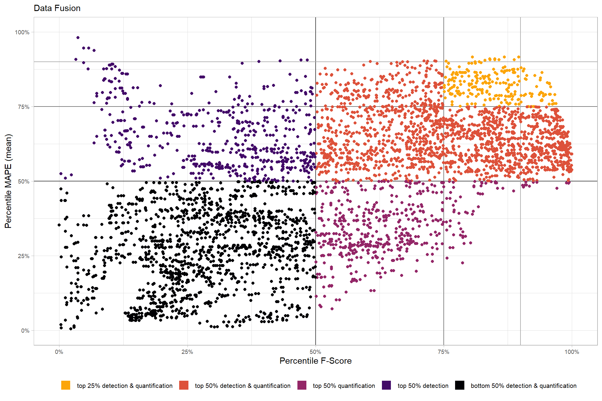
9.6.3.1.1 Top 1.0%
let’s check out the parameter settings of the top 1.0% (n=777) from all 77,760 combinations tested. these are “votes” for the parameter setting based on the combinations that achieved the best balance between both detection and quantification accuracy.
param_combos_spectral_ranked %>%
  dplyr::filter(is_top_overall) %>%
  dplyr::select(tidyselect::contains("f_score"), max_ht_m,max_area_m2,convexity_pct,circle_fit_iou_pct,chm_res_m,spectral_weight) %>%
  tidyr::pivot_longer(
    cols = c(max_ht_m,max_area_m2,convexity_pct,circle_fit_iou_pct,chm_res_m,spectral_weight)
    , names_to = "metric"
    , values_to = "value"
  ) %>%
  dplyr::count(metric, value) %>%
  dplyr::group_by(metric) %>%
  dplyr::mutate(
    pct=n/sum(n)
    , lab = paste0(scales::percent(pct,accuracy=0.1), "\nn=", scales::comma(n,accuracy=1))
  ) %>%
  ggplot2::ggplot(
    mapping = ggplot2::aes(x = factor(value), y=pct, label=lab, fill = metric)
  ) +
  ggplot2::geom_col(width = 0.6) +
  ggplot2::geom_text(color = "black", size = 2.5, vjust = -0.2) +
  ggplot2::facet_wrap(facets = dplyr::vars(metric), ncol=2, scales = "free_x") +
  ggplot2::scale_y_continuous(
    breaks = seq(0,1,by=0.2)
    , labels = scales::percent
    , expand = ggplot2::expansion(mult = c(0,0.2))
  ) +
  ggplot2::scale_fill_manual(values = pal_param[1:6]) +
  ggplot2::labs(
    x = "parameter setting", y = ""
    , fill = ""
    , subtitle = paste0(
      "Data Fusion"
       , "\nparameter settings of top "
       , scales::percent(pct_th_top,accuracy=0.1)
       , " (n="
       , scales::comma(sum(param_combos_spectral_ranked$is_top_overall), accuracy = 1)
       , ") "
       , "overall parameter combinations\nbased on both detection and quantification accuracy"
    )
  ) +
  ggplot2::theme_light() +
  ggplot2::theme(
    legend.position = "none"
    , strip.text = ggplot2::element_text(size = 11, color = "black", face = "bold")
    , axis.text.y = ggplot2::element_text(size = 6)
    , axis.text.x = ggplot2::element_text(size = 8)
    , plot.subtitle = ggplot2::element_text(size = 8)
  )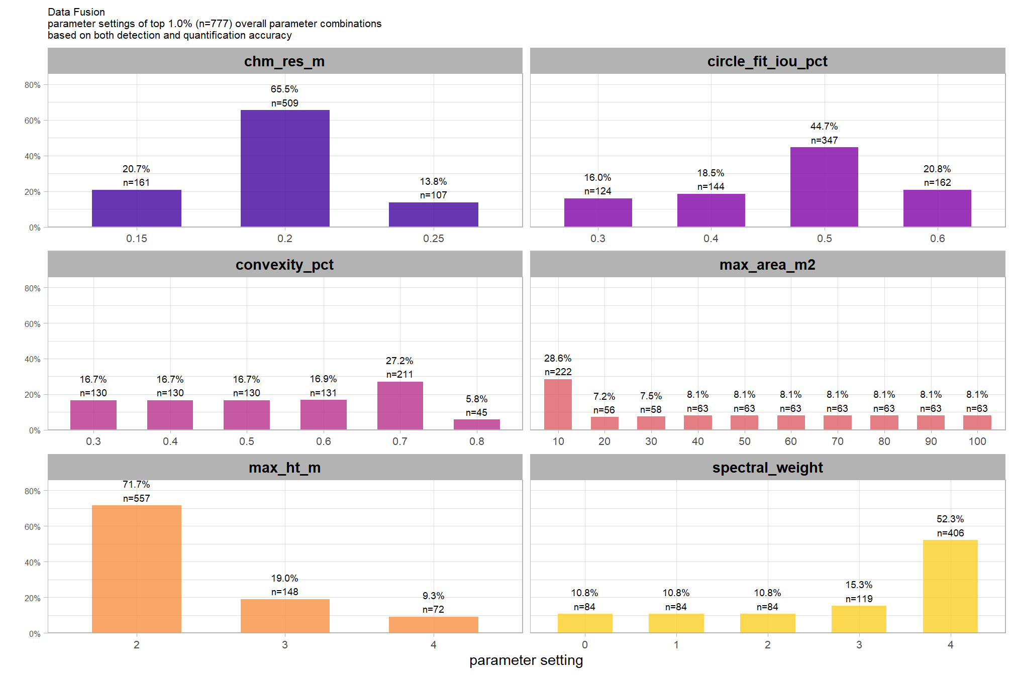
what is the expected detection accuracy of the top 1.0% (n=777) combinations tested?
plt_detection_dist(
  df = param_combos_spectral_ranked %>% dplyr::filter(is_top_overall) %>% dplyr::select(!tidyselect::contains("_pct_rank_"))
  , paste0(
    "Data Fusion"
    , "\ndistribution of evaluation metrics for top "
    , scales::percent(pct_th_top,accuracy=0.1)
    , " (n="
    , scales::comma(sum(param_combos_spectral_ranked$is_top_overall), accuracy = 1)
    , ") "
    , "overall parameter combinations\nbased on both detection and quantification accuracy"
  )
)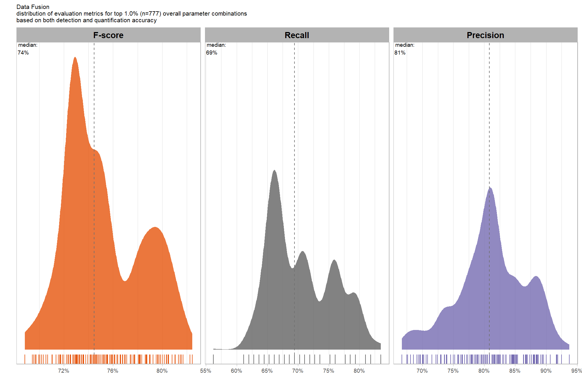
WHAT DID WE LEARN FROM THIS
what is the expected quantification accuracy of the top 1.0% (n=777) combinations tested?
# plot it
plt_form_quantification_dist(
  df = param_combos_spectral_ranked %>% dplyr::filter(is_top_overall) %>% dplyr::select(!tidyselect::contains("_pct_rank_"))
  , paste0(
    "Structural Data Only"
    , "\ndistribution of pile form quantification metrics for the top "
    , scales::percent(pct_th_top,accuracy=0.1)
    , " (n="
    , scales::comma(sum(param_combos_spectral_ranked$is_top_overall), accuracy = 1)
    , ") "
    , "overall parameter combinations\nbased on both detection and quantification accuracy"
  )
)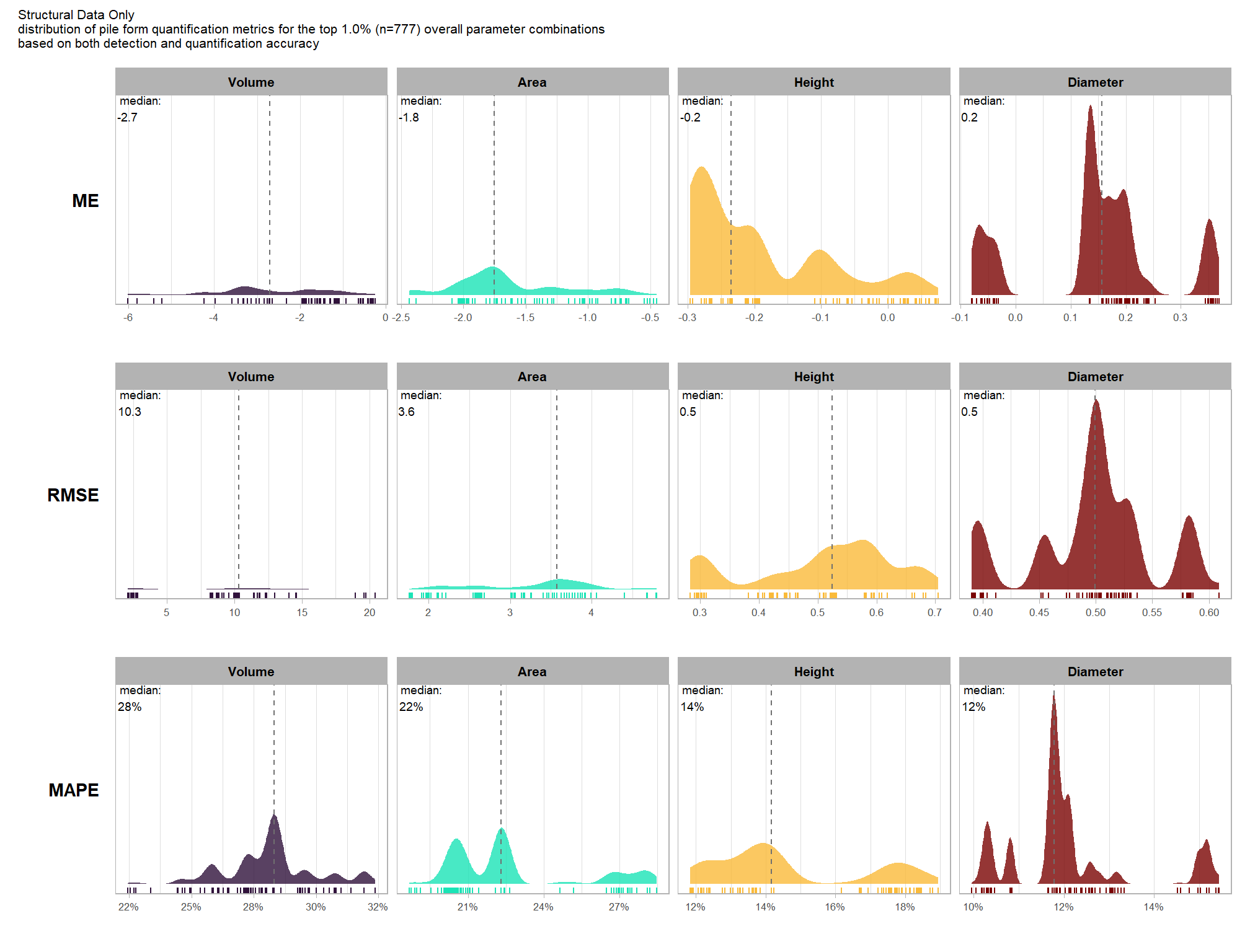
WHAT DID WE LEARN FROM THIS
9.6.3.1.2 Final 12 recommended settings
# pal_temp %>% scales::show_col()
# filter and reshape
param_combos_spectral_ranked %>%
  dplyr::filter(is_final_selection) %>%
  dplyr::select(!tidyselect::contains("_pct_rank_")) %>%
  dplyr::select(
    max_ht_m,max_area_m2,convexity_pct,circle_fit_iou_pct,chm_res_m,spectral_weight
    , ovrall_lab
    # detection
    , f_score, recall, precision
    # quantification
    , tidyselect::ends_with("_rmse")
    , tidyselect::ends_with("_rrmse")
    , tidyselect::ends_with("_mean")
    , tidyselect::ends_with("_mape")
  ) %>%
  tidyr::pivot_longer(
    cols = c(
      f_score, recall, precision
      , tidyselect::ends_with("_rmse")
      , tidyselect::ends_with("_rrmse")
      , tidyselect::ends_with("_mean")
      , tidyselect::ends_with("_mape")
    )
    , names_to = "metric"
    , values_to = "value"
  ) %>%
  dplyr::mutate(
    eval_metric = stringr::str_extract(metric, "(_rmse|_rrmse|_mean|_mape|f_score|recall|precision)$") %>%
      stringr::str_remove_all("_") %>%
      stringr::str_replace_all("mean","me") %>%
      toupper() %>%
      factor(
        ordered = T
        , levels = c("FSCORE","RECALL","PRECISION", "ME","RMSE","RRMSE","MAPE")
        , labels = c("F-score","Recall","Precision", "ME","RMSE","RRMSE","MAPE")
      )
    , pile_metric = metric %>%
      stringr::str_remove("(_rmse|_rrmse|_mean|_mape)$") %>%
      stringr::str_extract("(paraboloid_volume|volume|area|height|diameter)") %>%
      dplyr::coalesce("detection") %>%
      factor(
        ordered = T
        , levels = c(
          "detection"
          , "volume"
          , "paraboloid_volume"
          , "area"
          , "height"
          , "diameter"
        )
        , labels = c(
          "Detection"
          , "Volume"
          , "Volume paraboloid"
          , "Area"
          , "Height"
          , "Diameter"
        )
      )
    , value_lab = dplyr::case_when(
        eval_metric %in% c("F-score","Recall","Precision", "RRMSE", "MAPE") ~ scales::percent(value,accuracy=0.1)
        , eval_metric == "ME" ~ scales::comma(value,accuracy=0.01)
        , T ~ scales::comma(value,accuracy=0.1)
      )
  ) %>%
  # make var for color
  dplyr::group_by(pile_metric, eval_metric) %>%
  dplyr::mutate(
    # for ME, color by abs...for f-score,recall,precision color by -value so that higher means better...
      # ...since higher means worse for quantification accuracy metrics
    value_dir = dplyr::case_when(
      eval_metric %in% c("ME") ~ abs(value)
      , eval_metric %in% c("F-score","Recall","Precision") ~ -value
      , T ~ value
    )
    , value_z = (value_dir-mean(value_dir,na.rm=T))/sd(value_dir,na.rm=T) # this is the key to the different colors within facets
  ) %>%
  dplyr::ungroup() %>%
  dplyr::filter(!eval_metric %in% c("RRMSE")) %>%
  # View()
  ggplot2::ggplot(mapping = ggplot2::aes(x = eval_metric, y = ovrall_lab)) +
  ggplot2::geom_tile(
    mapping = ggplot2::aes(fill = pile_metric, alpha = -value_z)
    , color = "gray"
  ) +
  ggplot2::geom_text(
    mapping = ggplot2::aes(label = value_lab, fontface = "bold")
    , color = "white"
  ) +
  ggplot2::facet_grid(cols = dplyr::vars(pile_metric), scales = "free_x") +
  ggplot2::scale_x_discrete(position = "top") +
  ggplot2::scale_fill_manual(values = c("gray33", viridis::turbo(n=4))) +
  ggplot2::scale_alpha_binned(range = c(0.55, 1)) + # this is the key to the different colors within facets
  ggplot2::theme_light() +
  ggplot2::labs(
    x = ""
    , y = "max_ht_m : max_area_m2 : convexity_pct : circle_fit_iou_pct : chm_res_m : spectral_weight"
    , subtitle = paste0(
       "Data Fusion"
       , "\npile detection and form quantification accuracy metrics for the final recommended parameter settings"
       # , scales::percent(1-pct_rank_th_top,accuracy=1)
       , " (n="
       , scales::comma(n_th_top,accuracy=1)
       , ") "
       , "\nbased on both detection and quantification accuracy"
      )
    , caption = "*darker colors indicate relatively higher accuracy values"
  ) +
  ggplot2::theme(
    legend.position = "none"
    , panel.grid = ggplot2::element_blank()
    , strip.placement = "outside"
    , strip.text.x = ggplot2::element_text(size = 8, color = "black", face = "bold")
    , axis.text.x = ggplot2::element_text(size = 7, color = "black", face = "bold")
    , axis.title.x = ggplot2::element_blank()
    , plot.subtitle = ggplot2::element_text(size = 8)
  )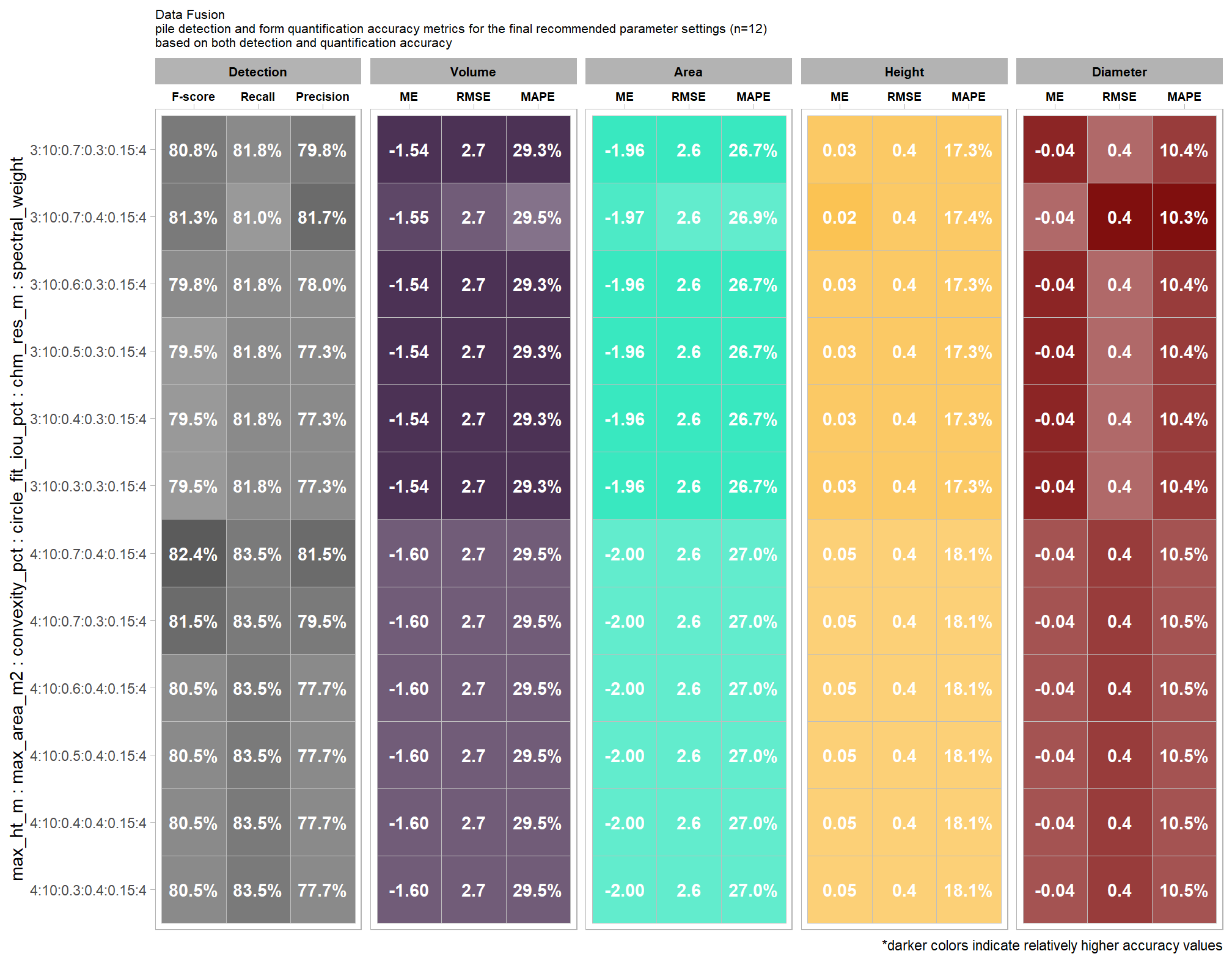
this plot allows for a simultaneous comparison of all metrics for pile detection and pile form quantification. it includes only the parameter combinations that achieved the best balanced accuracy, helping users identify the optimal settings by evaluating the trade-offs between detection and form quantification.
let’s table this
param_combos_spectral_ranked %>%
  dplyr::filter(is_final_selection) %>%
  dplyr::select(!tidyselect::contains("_pct_rank_")) %>%
  # first select to arrange eval_metric
  dplyr::select(
    ovrall_lab
    , max_ht_m,max_area_m2,convexity_pct,circle_fit_iou_pct,chm_res_m,spectral_weight
    # detection
    , f_score, recall, precision
    # quantification
    , tidyselect::ends_with("_mean")
    , tidyselect::ends_with("_rmse")
    # , tidyselect::ends_with("_rrmse")
    , tidyselect::ends_with("_mape")
  ) %>%
  # second select to arrange pile_metric
  dplyr::select(
    ovrall_lab
    , max_ht_m,max_area_m2,convexity_pct,circle_fit_iou_pct,chm_res_m,spectral_weight
    # detection
    , f_score, recall, precision
    # quantification
    , c(tidyselect::contains("volume") & !tidyselect::contains("paraboloid"))
    , tidyselect::contains("area")
    , tidyselect::contains("height")
    , tidyselect::contains("diameter")
  ) %>%
  # names()
  dplyr::mutate(
    dplyr::across(
      .cols = c(f_score, recall, precision, tidyselect::ends_with("_mape"))
      , .fn = ~ scales::percent(.x, accuracy = 1)
    )
    , dplyr::across(
      .cols = c(tidyselect::ends_with("_mean"))
      , .fn = ~ scales::comma(.x, accuracy = 0.01)
    )
    , dplyr::across(
      .cols = c(tidyselect::ends_with("_rmse"))
      , .fn = ~ scales::comma(.x, accuracy = 0.1)
    )
  ) %>%
  dplyr::mutate(blank= "   " ) %>%
  dplyr::relocate(blank, .before = f_score) %>%
  dplyr::arrange(desc(ovrall_lab)) %>%
  kableExtra::kbl(
    caption =
      paste0(
       "Data Fusion"
       , "<br>pile detection and form quantification accuracy metrics for the final recommended parameter settings"
       # , scales::percent(1-pct_rank_th_top,accuracy=1)
       , " (n="
       , scales::comma(n_th_top,accuracy=1)
       , ") "
       , "<br>based on both detection and quantification accuracy"
      )
    , col.names = c(
      ""
      ,"max_ht_m","max_area_m2","convexity_pct","circle_fit_iou_pct","chm_res_m","spectral_weight"
      , "   "
      , "F-score", "Recall", "Precision"
      , rep(c("ME","RMSE","MAPE"), times = 4)
    )
    , escape = F
  ) %>%
  kableExtra::kable_styling(font_size = 11) %>%
  kableExtra::add_header_above(c(
    " "=8
    , "Detection" = 3
    , "Volume" = 3
    , "Area" = 3
    , "Height" = 3
    , "Diameter" = 3
  )) %>%
  kableExtra::column_spec(seq(8,23,by=3), border_right = TRUE, include_thead = TRUE) %>%
  kableExtra::column_spec(
    column = 8:23
    , extra_css = "font-size: 10px;"
    , include_thead = T
  ) %>%
kableExtra::scroll_box(width = "740px") | max_ht_m | max_area_m2 | convexity_pct | circle_fit_iou_pct | chm_res_m | spectral_weight | F-score | Recall | Precision | ME | RMSE | MAPE | ME | RMSE | MAPE | ME | RMSE | MAPE | ME | RMSE | MAPE | ||
|---|---|---|---|---|---|---|---|---|---|---|---|---|---|---|---|---|---|---|---|---|---|---|
| 3:10:0.7:0.3:0.15:4 | 3 | 10 | 0.7 | 0.3 | 0.15 | 4 | 81% | 82% | 80% | -1.54 | 2.7 | 29% | -1.96 | 2.6 | 27% | 0.03 | 0.4 | 17% | -0.04 | 0.4 | 10% | |
| 3:10:0.7:0.4:0.15:4 | 3 | 10 | 0.7 | 0.4 | 0.15 | 4 | 81% | 81% | 82% | -1.55 | 2.7 | 30% | -1.97 | 2.6 | 27% | 0.02 | 0.4 | 17% | -0.04 | 0.4 | 10% | |
| 3:10:0.6:0.3:0.15:4 | 3 | 10 | 0.6 | 0.3 | 0.15 | 4 | 80% | 82% | 78% | -1.54 | 2.7 | 29% | -1.96 | 2.6 | 27% | 0.03 | 0.4 | 17% | -0.04 | 0.4 | 10% | |
| 3:10:0.5:0.3:0.15:4 | 3 | 10 | 0.5 | 0.3 | 0.15 | 4 | 80% | 82% | 77% | -1.54 | 2.7 | 29% | -1.96 | 2.6 | 27% | 0.03 | 0.4 | 17% | -0.04 | 0.4 | 10% | |
| 3:10:0.4:0.3:0.15:4 | 3 | 10 | 0.4 | 0.3 | 0.15 | 4 | 80% | 82% | 77% | -1.54 | 2.7 | 29% | -1.96 | 2.6 | 27% | 0.03 | 0.4 | 17% | -0.04 | 0.4 | 10% | |
| 3:10:0.3:0.3:0.15:4 | 3 | 10 | 0.3 | 0.3 | 0.15 | 4 | 80% | 82% | 77% | -1.54 | 2.7 | 29% | -1.96 | 2.6 | 27% | 0.03 | 0.4 | 17% | -0.04 | 0.4 | 10% | |
| 4:10:0.7:0.4:0.15:4 | 4 | 10 | 0.7 | 0.4 | 0.15 | 4 | 82% | 83% | 81% | -1.60 | 2.7 | 29% | -2.00 | 2.6 | 27% | 0.05 | 0.4 | 18% | -0.04 | 0.4 | 10% | |
| 4:10:0.7:0.3:0.15:4 | 4 | 10 | 0.7 | 0.3 | 0.15 | 4 | 81% | 83% | 80% | -1.60 | 2.7 | 29% | -2.00 | 2.6 | 27% | 0.05 | 0.4 | 18% | -0.04 | 0.4 | 10% | |
| 4:10:0.6:0.4:0.15:4 | 4 | 10 | 0.6 | 0.4 | 0.15 | 4 | 80% | 83% | 78% | -1.60 | 2.7 | 29% | -2.00 | 2.6 | 27% | 0.05 | 0.4 | 18% | -0.04 | 0.4 | 10% | |
| 4:10:0.5:0.4:0.15:4 | 4 | 10 | 0.5 | 0.4 | 0.15 | 4 | 80% | 83% | 78% | -1.60 | 2.7 | 29% | -2.00 | 2.6 | 27% | 0.05 | 0.4 | 18% | -0.04 | 0.4 | 10% | |
| 4:10:0.4:0.4:0.15:4 | 4 | 10 | 0.4 | 0.4 | 0.15 | 4 | 80% | 83% | 78% | -1.60 | 2.7 | 29% | -2.00 | 2.6 | 27% | 0.05 | 0.4 | 18% | -0.04 | 0.4 | 10% | |
| 4:10:0.3:0.4:0.15:4 | 4 | 10 | 0.3 | 0.4 | 0.15 | 4 | 80% | 83% | 78% | -1.60 | 2.7 | 29% | -2.00 | 2.6 | 27% | 0.05 | 0.4 | 18% | -0.04 | 0.4 | 10% |
what is the expected detection accuracy of the final 12 recommended settings?
plt_detection_dist(
  df = param_combos_spectral_ranked %>% dplyr::filter(is_final_selection) %>% dplyr::select(!tidyselect::contains("_pct_rank_"))
  , paste0(
    "Data Fusion"
    , "\ndistribution of evaluation metrics for the final recommended parameter settings"
    , " (n="
    , scales::comma(n_th_top,accuracy=1)
    , ") "
    , "\nbased on both detection and quantification accuracy"
  )
)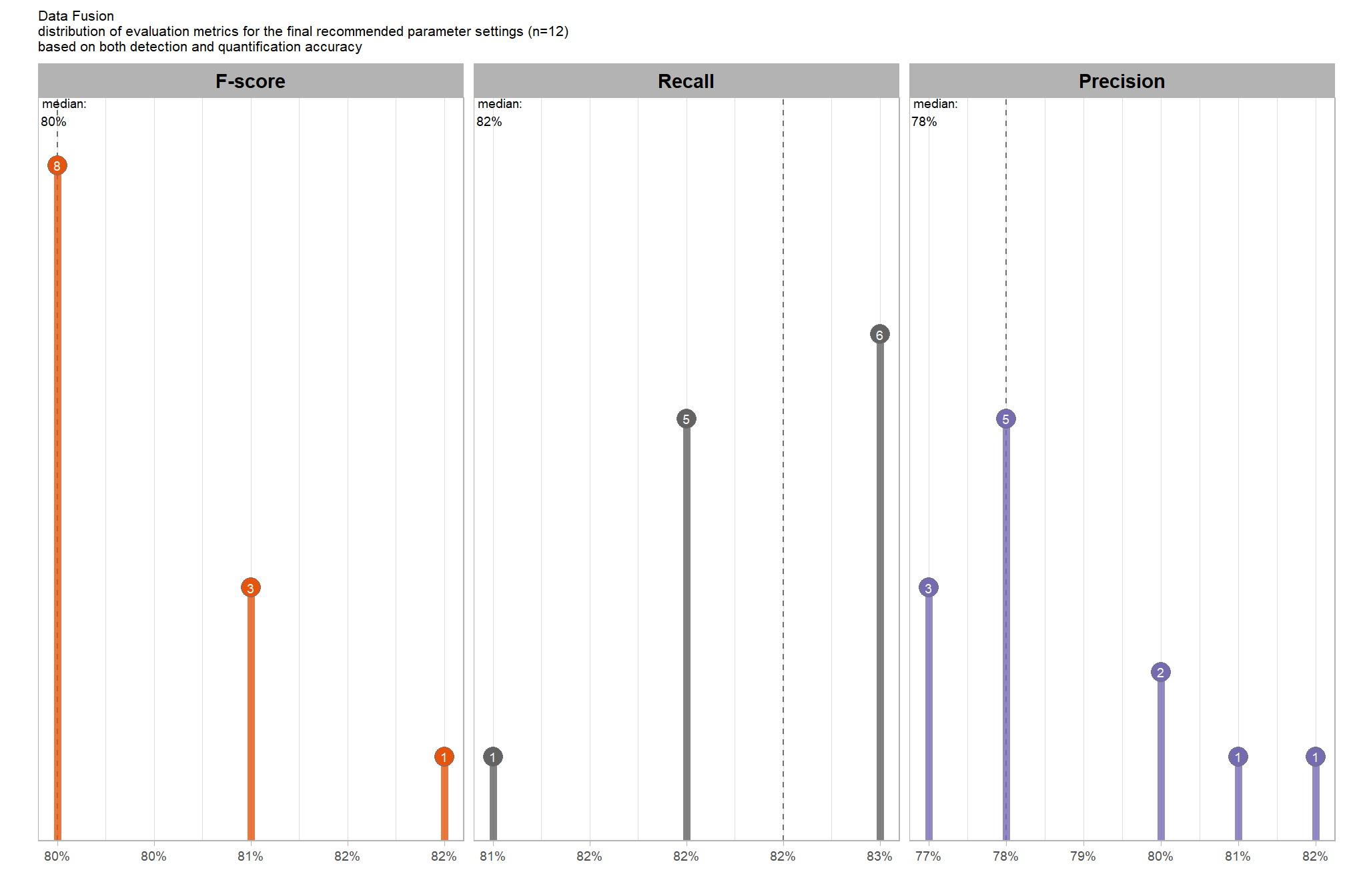
WHAT DID WE LEARN FROM THIS
what is the expected quantification accuracy of the final 12 recommended settings?
# plot it
plt_form_quantification_dist(
  df = param_combos_spectral_ranked %>% dplyr::filter(is_final_selection) %>% dplyr::select(!tidyselect::contains("_pct_rank_"))
  , paste0(
    "Data Fusion"
    , "\ndistribution of pile form quantification metrics for the final recommended parameter settings"
    , " (n="
    , scales::comma(n_th_top,accuracy=1)
    , ") "
    , "\nbased on both detection and quantification accuracy"
  )
)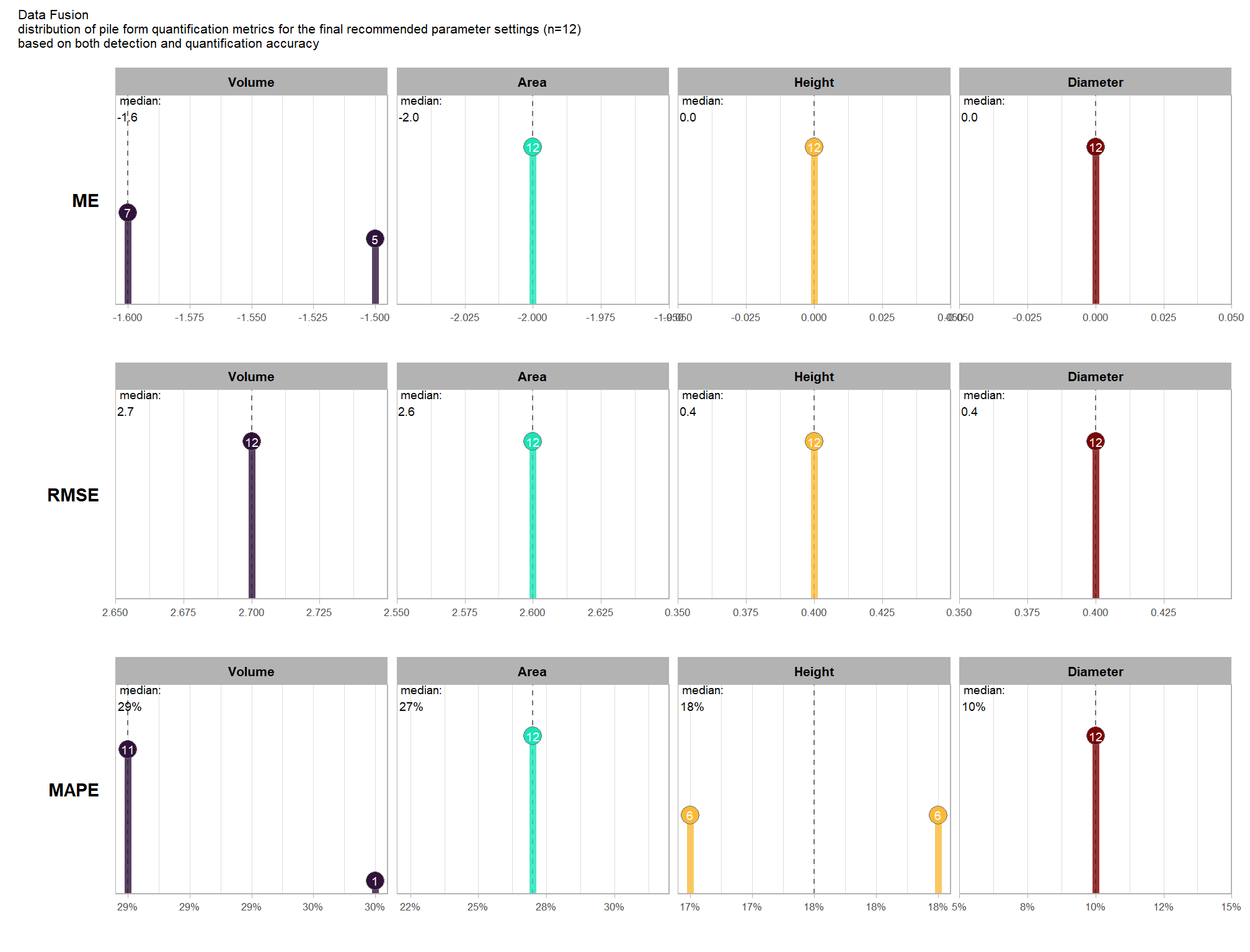
WHAT DID WE LEARN FROM THIS
finally, here are the combinations selected compared against all 77,760 combinations tested.
dplyr::bind_rows(
  param_combos_spectral_ranked %>% dplyr::filter(is_final_selection)
  , param_combos_spectral_ranked %>% dplyr::filter(!is_final_selection) %>% dplyr::slice_sample(prop = (1/6))
) %>%
  dplyr::select(
    rn,max_ht_m,max_area_m2,convexity_pct,circle_fit_iou_pct
    , is_final_selection
    , f_score, precision, recall
    # quantification accuracy
    , tidyselect::ends_with("_mape")
  ) %>%
  tidyr::pivot_longer(
    cols = c(
      tidyselect::ends_with("_mape")
      # ,precision,recall
    )
    , names_to = "metric"
    , values_to = "value"
  ) %>%
  dplyr::mutate(
    eval_metric = stringr::str_extract(metric, "(_rmse|_rrmse|_mean|_mape)$") %>%
      stringr::str_remove_all("_") %>%
      stringr::str_replace_all("mean","me") %>%
      toupper() %>%
      factor(
        ordered = T
        , levels = c("ME","RMSE","RRMSE","MAPE")
      )
    , pile_metric = metric %>%
      stringr::str_remove("(_rmse|_rrmse|_mean|_mape)$") %>%
      stringr::str_extract("(paraboloid_volume|volume|area|height|diameter|precision|recall)") %>%
      factor(
        ordered = T
        , levels = c(
          "volume"
          , "paraboloid_volume"
          , "area"
          , "height"
          , "diameter"
          , "recall"
          , "precision"
        )
        , labels = c(
          "Volume"
          , "Volume paraboloid"
          , "Area"
          , "Height"
          , "Diameter"
          , "Recall"
          , "Precision"
        )
      )
    , color_metric = ifelse(is_final_selection, pile_metric, NA) %>% factor()
  ) %>%
  dplyr::arrange(is_final_selection) %>%
  # plot
  ggplot2::ggplot(mapping = ggplot2::aes(x = f_score, y = value, color = color_metric)) +
  ggplot2::geom_point() +
  ggplot2::facet_wrap(facets = dplyr::vars(pile_metric)) +
  ggplot2::scale_color_viridis_d(option = "turbo", na.value = "gray88") +
  ggplot2::scale_x_continuous(
    labels = scales::percent_format(accuracy = 1)
    , limits = c(0,1)
  ) +
  ggplot2::scale_y_continuous(
    labels = scales::percent_format(accuracy = 1)
    , limits = c(0,NA)
  ) +
  ggplot2::labs(x = "F-Score", y = "MAPE", caption = "*records in gray not selected") +
  ggplot2::theme_light() +
  ggplot2::theme(
    legend.position = "none"
    , strip.text = ggplot2::element_text(size = 11, color = "black", face = "bold")
  )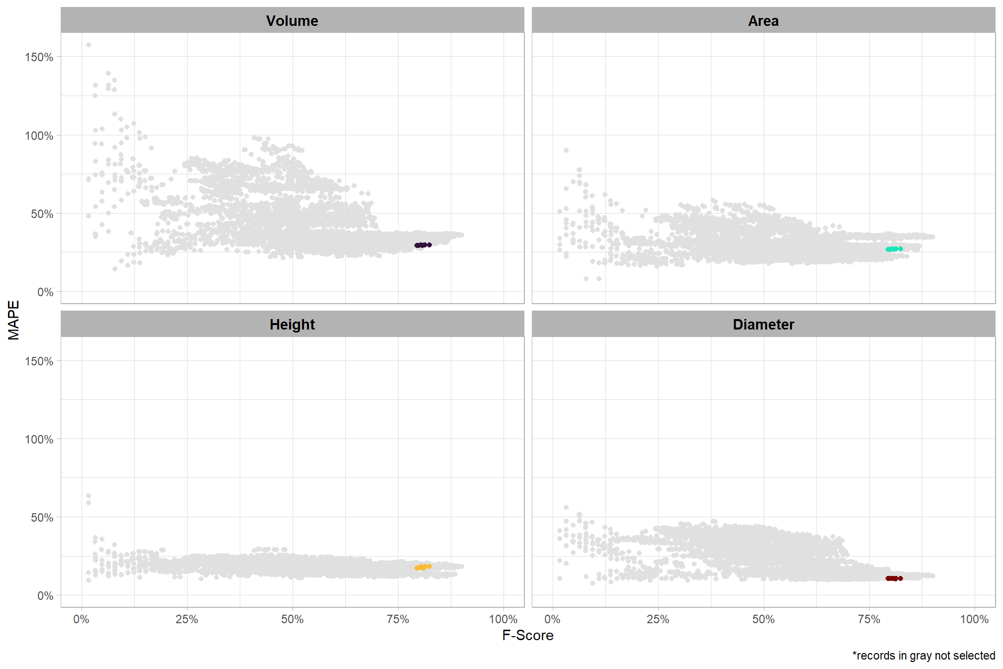
WHAT DID WE LEARN FROM THIS
9.6.3.2 by CHM resolution
To select the best-performing parameter combinations, we will prioritize those that balance detection and quantification accuracy. From this group, we will then identify the settings that achieve the highest pile detection rates (recall). These recommendations are for users who are working with a CHM with a resolution in the range of those tested for this analysis or can aggregate (i.e. make more coarse) a CHM to a resolution tested for the purpose of either improving processing performance or enhancing pile detection and/or quantification accuracy based on the results shown here
we already created this data above (param_combos_ranked) using the F-Score and the average rank of the MAPE metrics across all form measurements (i.e. height, diameter, area, volume) to determine the best overall list by CHM resolution
9.6.3.2.1 Top 2.0%
let’s check out the parameter settings of the top 2.0% (n=172) from all 8,640 combinations tested by CHM resolution. these are “votes” for the parameter setting based on the combinations that achieved the best balance between both detection and quantification accuracy.
param_combos_spectral_ranked %>%
  dplyr::filter(is_top_chm) %>%
  dplyr::select(tidyselect::contains("f_score"), max_ht_m,max_area_m2,convexity_pct,circle_fit_iou_pct,chm_res_m,chm_res_m_desc,spectral_weight) %>%
  tidyr::pivot_longer(
    cols = c(max_ht_m,max_area_m2,convexity_pct,circle_fit_iou_pct,spectral_weight)
    , names_to = "metric"
    , values_to = "value"
  ) %>%
  dplyr::count(chm_res_m,chm_res_m_desc, metric, value) %>%
  dplyr::group_by(chm_res_m,chm_res_m_desc, metric) %>%
  dplyr::mutate(
    pct=n/sum(n)
    , lab = paste0(scales::percent(pct,accuracy=0.1)) #, "\nn=", scales::comma(n,accuracy=1))
  ) %>%
  ggplot2::ggplot(
    mapping = ggplot2::aes(x = factor(value), y=pct, label=lab, fill = metric)
  ) +
  ggplot2::geom_col(width = 0.6) +
  ggplot2::geom_text(color = "black", size = 2.2, vjust = -0.2) +
  ggplot2::facet_grid(cols = dplyr::vars(metric), rows = dplyr::vars(chm_res_m_desc), scales = "free_x") +
  ggplot2::scale_y_continuous(
    breaks = seq(0,1,by=0.2)
    , labels = scales::percent
    , expand = ggplot2::expansion(mult = c(0,0.2))
  ) +
  ggplot2::scale_fill_manual(values = pal_param[c(1:4,6)]) +
  ggplot2::labs(
    x = "parameter setting", y = ""
    , fill = ""
    , subtitle = paste0(
      "Data Fusion"
       , "\nparameter settings of top "
       , scales::percent(pct_th_top_chm,accuracy=0.1)
       , " (n="
       , scales::comma(n_combos_top_spectral_chm , accuracy = 1)
       , ") "
       , "parameter combinations by CHM resolution\nbased on both detection and quantification accuracy"
    )
  ) +
  ggplot2::theme_light() +
  ggplot2::theme(
    legend.position = "none"
    , strip.text.x = ggplot2::element_text(size = 11, color = "black", face = "bold")
    , strip.text.y = ggplot2::element_text(size = 9, color = "black", face = "bold")
    , axis.text.y = ggplot2::element_text(size = 6)
    , axis.text.x = ggplot2::element_text(size = 8)
    , plot.subtitle = ggplot2::element_text(size = 8)
  )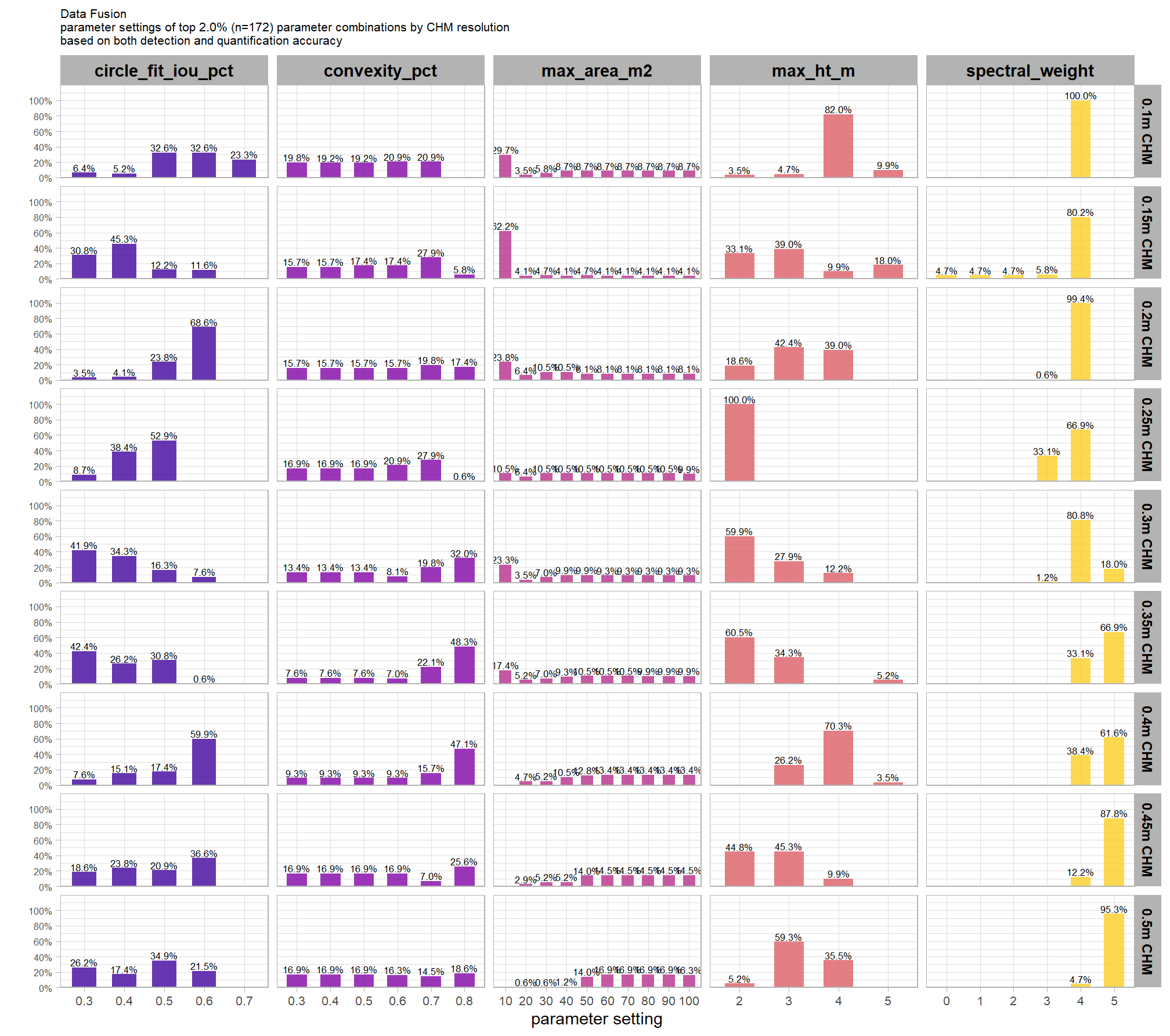
what is the expected detection accuracy of the top 2.0% (n=172) combinations tested by CHM resolution?
plt_detection_dist2(
  df = param_combos_spectral_ranked %>% dplyr::filter(is_top_chm) %>% dplyr::select(!tidyselect::contains("_pct_rank_"))
  , paste0(
    "Data Fusion"
    , "\ndistribution of evaluation metrics for top "
    , scales::percent(pct_th_top_chm,accuracy=0.1)
    , " (n="
    , scales::comma(n_combos_top_spectral_chm, accuracy=1)
    , ") "
    , "parameter combinations by CHM resolution\nbased on both detection and quantification accuracy"
  )
)
WHAT DID WE LEARN FROM THIS
what is the expected MAPE of the top 2.0% (n=172) combinations tested by CHM resolution?
# plot it
plt_form_quantification_dist2(
  df = param_combos_spectral_ranked %>% dplyr::filter(is_top_chm) %>% dplyr::select(!tidyselect::contains("_pct_rank_"))
  , quant_metric = "mape"
  , paste0(
    "Data Fusion"
    , "\ndistribution of pile form quantification metrics for the top "
    , scales::percent(pct_th_top_chm,accuracy=0.1)
    , " (n="
    , scales::comma(n_combos_top_spectral_chm, accuracy=1)
    , ") "
    , "parameter combinations by CHM resolution\nbased on both detection and quantification accuracy"
  )
)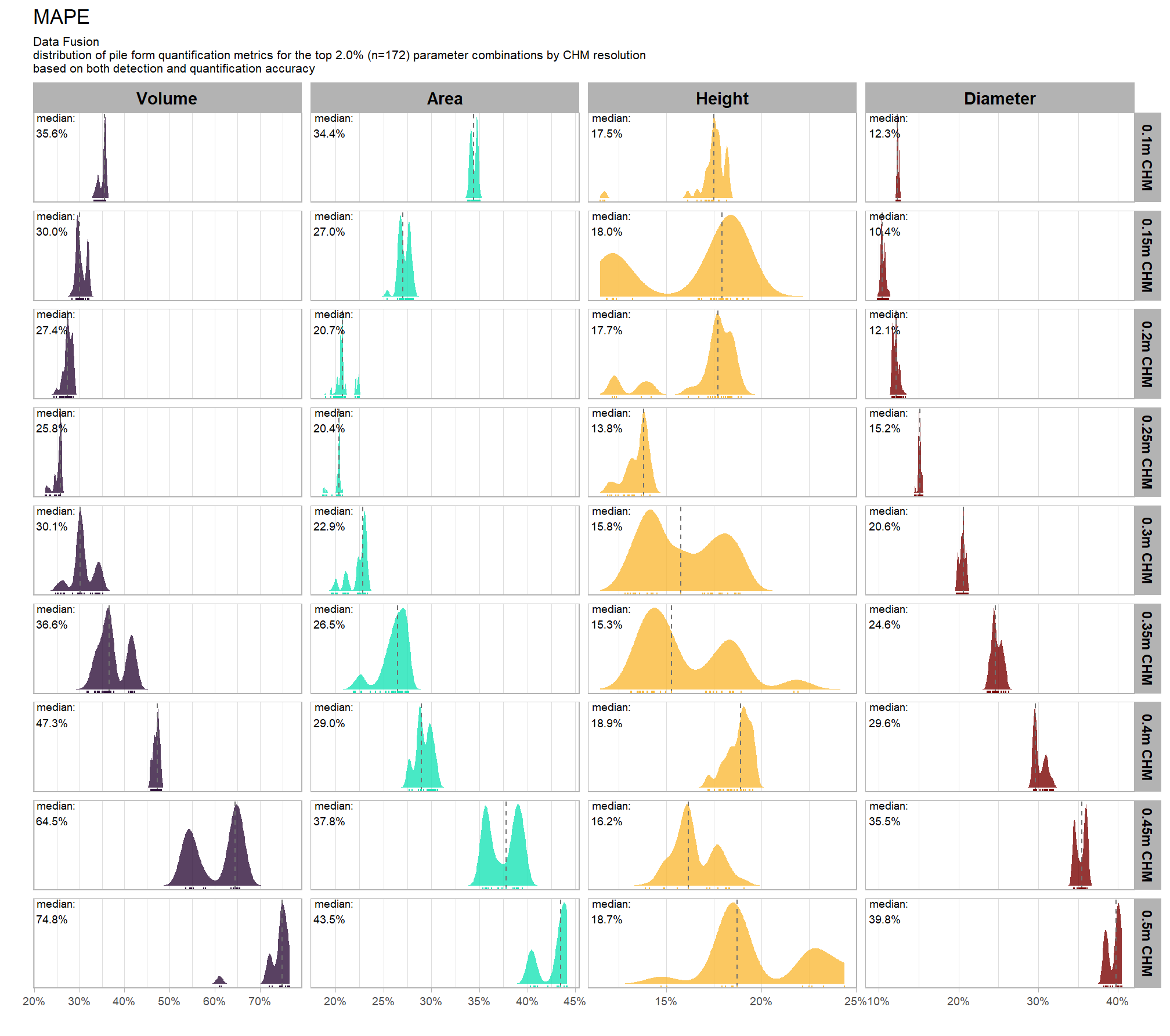
WHAT DID WE LEARN FROM THIS
what is the expected Mean Error (ME) of the top 2.0% (n=172) combinations tested by CHM resolution?
# plot it
plt_form_quantification_dist2(
  df = param_combos_spectral_ranked %>% dplyr::filter(is_top_chm) %>% dplyr::select(!tidyselect::contains("_pct_rank_"))
  , quant_metric = "mean"
  , paste0(
    "Data Fusion"
    , "\ndistribution of pile form quantification metrics for the top "
    , scales::percent(pct_th_top_chm,accuracy=0.1)
    , " (n="
    , scales::comma(n_combos_top_spectral_chm, accuracy=1)
    , ") "
    , "parameter combinations by CHM resolution\nbased on both detection and quantification accuracy"
  )
)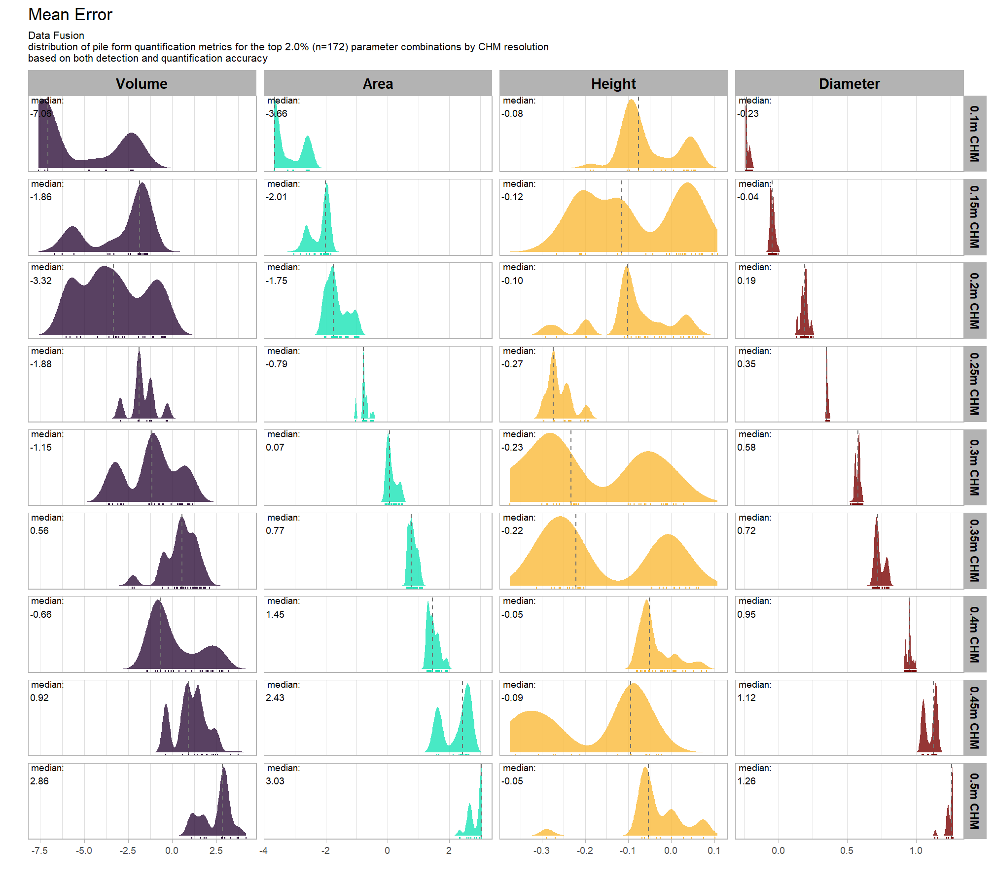
WHAT DID WE LEARN FROM THIS
what is the expected RMSE of the top 2.0% (n=172) combinations tested by CHM resolution?
# plot it
plt_form_quantification_dist2(
  df = param_combos_spectral_ranked %>% dplyr::filter(is_top_chm) %>% dplyr::select(!tidyselect::contains("_pct_rank_"))
  , quant_metric = "rmse"
  , paste0(
    "Data Fusion"
    , "\ndistribution of pile form quantification metrics for the top "
    , scales::percent(pct_th_top_chm,accuracy=0.1)
    , " (n="
    , scales::comma(n_combos_top_spectral_chm, accuracy=1)
    , ") "
    , "parameter combinations by CHM resolution\nbased on both detection and quantification accuracy"
  )
)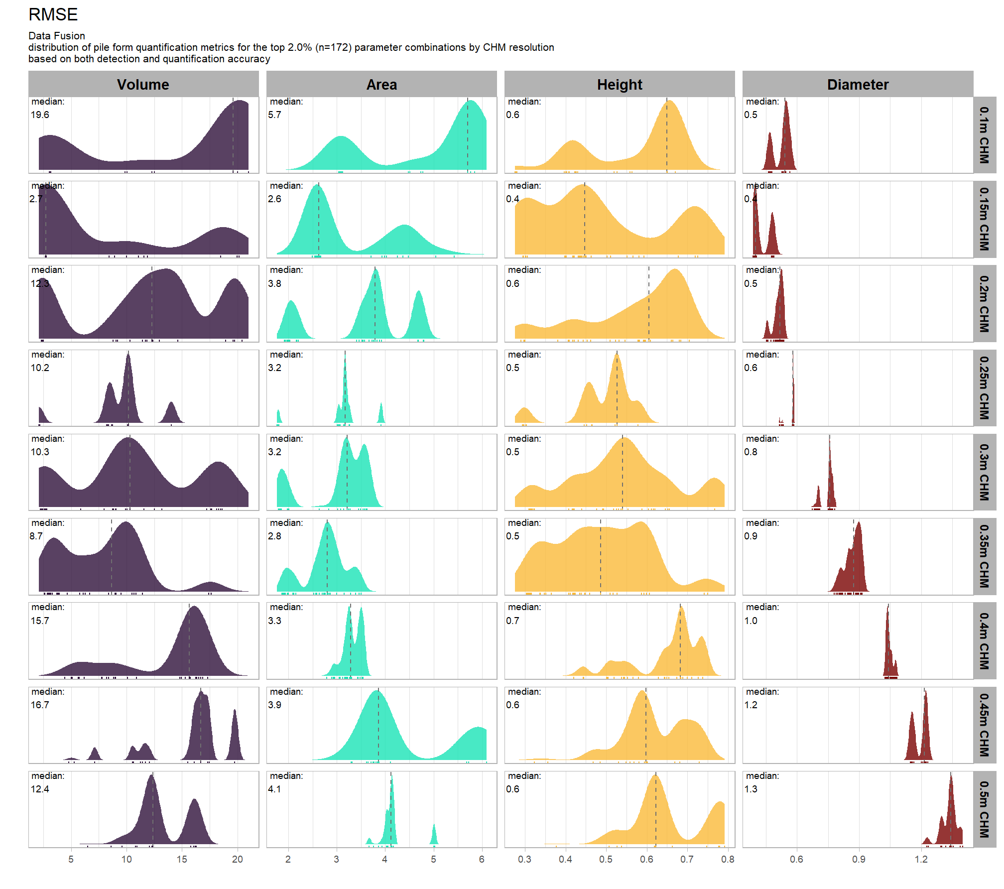
WHAT DID WE LEARN FROM THIS
9.6.3.2.2 Final 6 recommended settings
# pal_temp %>% scales::show_col()
# filter and reshape
param_combos_spectral_ranked %>%
  dplyr::filter(is_final_selection_chm) %>%
  dplyr::select(!tidyselect::contains("_pct_rank_")) %>%
  dplyr::select(
    max_ht_m,max_area_m2,convexity_pct,circle_fit_iou_pct,chm_res_m,chm_res_m_desc,spectral_weight
    , chm_lab
    # detection
    , f_score, recall, precision
    # quantification
    , tidyselect::ends_with("_rmse")
    , tidyselect::ends_with("_rrmse")
    , tidyselect::ends_with("_mean")
    , tidyselect::ends_with("_mape")
  ) %>%
  tidyr::pivot_longer(
    cols = c(
      f_score, recall, precision
      , tidyselect::ends_with("_rmse")
      , tidyselect::ends_with("_rrmse")
      , tidyselect::ends_with("_mean")
      , tidyselect::ends_with("_mape")
    )
    , names_to = "metric"
    , values_to = "value"
  ) %>%
  dplyr::mutate(
    eval_metric = stringr::str_extract(metric, "(_rmse|_rrmse|_mean|_mape|f_score|recall|precision)$") %>%
      stringr::str_remove_all("_") %>%
      stringr::str_replace_all("mean","me") %>%
      toupper() %>%
      factor(
        ordered = T
        , levels = c("FSCORE","RECALL","PRECISION", "ME","RMSE","RRMSE","MAPE")
        , labels = c("F-score","Recall","Precision", "ME","RMSE","RRMSE","MAPE")
      )
    , pile_metric = metric %>%
      stringr::str_remove("(_rmse|_rrmse|_mean|_mape)$") %>%
      stringr::str_extract("(paraboloid_volume|volume|area|height|diameter)") %>%
      dplyr::coalesce("detection") %>%
      factor(
        ordered = T
        , levels = c(
          "detection"
          , "volume"
          , "paraboloid_volume"
          , "area"
          , "height"
          , "diameter"
        )
        , labels = c(
          "Detection"
          , "Volume"
          , "Volume paraboloid"
          , "Area"
          , "Height"
          , "Diameter"
        )
      )
    , value_lab = dplyr::case_when(
        eval_metric %in% c("F-score","Recall","Precision", "RRMSE", "MAPE") ~ scales::percent(value,accuracy=0.1)
        , eval_metric == "ME" ~ scales::comma(value,accuracy=0.01)
        , T ~ scales::comma(value,accuracy=0.1)
      )
  ) %>%
  # make var for color
  dplyr::group_by(chm_res_m,chm_res_m_desc, pile_metric, eval_metric) %>%
  dplyr::mutate(
    # for ME, color by abs...for f-score,recall,precision color by -value so that higher means better...
      # ...since higher means worse for quantification accuracy metrics
    value_dir = dplyr::case_when(
      eval_metric %in% c("ME") ~ abs(value)
      , eval_metric %in% c("F-score","Recall","Precision") ~ -value
      , T ~ value
    )
    , value_z = (value_dir-mean(value_dir,na.rm=T))/sd(value_dir,na.rm=T) # this is the key to the different colors within facets
  ) %>%
  dplyr::ungroup() %>%
  dplyr::filter(!eval_metric %in% c("RRMSE")) %>%
  # View()
  ggplot2::ggplot(mapping = ggplot2::aes(x = eval_metric, y = chm_lab)) +
  ggplot2::geom_tile(
    mapping = ggplot2::aes(fill = pile_metric, alpha = -value_z)
    , color = "gray"
  ) +
  ggplot2::geom_text(
    mapping = ggplot2::aes(label = value_lab, fontface = "bold")
    , color = "white"
    , size = 3
  ) +
  ggplot2::facet_grid(cols = dplyr::vars(pile_metric), rows = dplyr::vars(chm_res_m_desc), scales = "free") +
  ggplot2::scale_x_discrete(position = "top") +
  ggplot2::scale_fill_manual(values = c("gray33", viridis::turbo(n=4))) +
  ggplot2::scale_alpha_binned(range = c(0.55, 1)) + # this is the key to the different colors within facets
  ggplot2::theme_light() +
  ggplot2::labs(
    x = ""
    , y = "max_ht_m : max_area_m2 : convexity_pct : circle_fit_iou_pct : chm_res_m : spectral_weight"
    , subtitle = paste0(
       "Data Fusion"
       , "\npile detection and form quantification accuracy metrics for the final recommended parameter settings"
       # , scales::percent(1-pct_rank_th_top,accuracy=1)
       , " (n="
       , scales::comma(n_th_top_chm,accuracy=1)
       , ") by CHM resolution"
       , "\nbased on both detection and quantification accuracy"
      )
    , caption = "*darker colors indicate relatively higher accuracy values"
  ) +
  ggplot2::theme(
    legend.position = "none"
    , panel.grid = ggplot2::element_blank()
    , strip.placement = "outside"
    , strip.text.x = ggplot2::element_text(size = 8, color = "black", face = "bold")
    , strip.text.y = ggplot2::element_text(size = 9, color = "black", face = "bold")
    , axis.text.x = ggplot2::element_text(size = 7, color = "black", face = "bold")
    , axis.text.y = ggplot2::element_text(size = 7)
    , axis.title.x = ggplot2::element_blank()
    , plot.subtitle = ggplot2::element_text(size = 8)
  )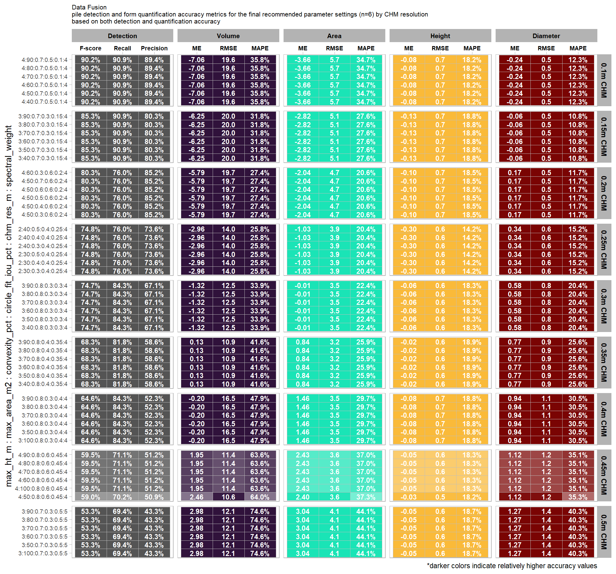
this plot allows for a simultaneous comparison of all metrics for pile detection and pile form quantification. it includes only the parameter combinations that achieved the best balanced accuracy, helping users identify the optimal settings by evaluating the trade-offs between detection and form quantification.
let’s table this
param_combos_spectral_ranked %>%
  dplyr::filter(is_final_selection_chm) %>%
  dplyr::select(!tidyselect::contains("_pct_rank_")) %>%
  # first select to arrange eval_metric
  dplyr::select(
    chm_lab, chm_res_m_desc
    , max_ht_m,max_area_m2,convexity_pct,circle_fit_iou_pct,chm_res_m,spectral_weight
    # detection
    , f_score, recall, precision
    # quantification
    , tidyselect::ends_with("_mean")
    , tidyselect::ends_with("_rmse")
    # , tidyselect::ends_with("_rrmse")
    , tidyselect::ends_with("_mape")
  ) %>%
  # second select to arrange pile_metric
  dplyr::select(
    chm_lab, chm_res_m_desc
    , max_ht_m,max_area_m2,convexity_pct,circle_fit_iou_pct,chm_res_m,spectral_weight
    # detection
    , f_score, recall, precision
    # quantification
    , c(tidyselect::contains("volume") & !tidyselect::contains("paraboloid"))
    , tidyselect::contains("area")
    , tidyselect::contains("height")
    , tidyselect::contains("diameter")
  ) %>%
  # names()
  dplyr::mutate(
    dplyr::across(
      .cols = c(f_score, recall, precision, tidyselect::ends_with("_mape"))
      , .fn = ~ scales::percent(.x, accuracy = 1)
    )
    , dplyr::across(
      .cols = c(tidyselect::ends_with("_mean"))
      , .fn = ~ scales::comma(.x, accuracy = 0.01)
    )
    , dplyr::across(
      .cols = c(tidyselect::ends_with("_rmse"))
      , .fn = ~ scales::comma(.x, accuracy = 0.1)
    )
  ) %>%
  dplyr::mutate(blank= "   " ) %>%
  dplyr::relocate(blank, .before = f_score) %>%
  dplyr::arrange(chm_res_m, desc(chm_lab)) %>%
  dplyr::select(-chm_res_m) %>%
  dplyr::relocate(chm_res_m_desc) %>%
  kableExtra::kbl(
    caption =
      paste0(
       "Data Fusion"
       , "<br>pile detection and form quantification accuracy metrics for the final recommended parameter settings"
       # , scales::percent(1-pct_rank_th_top,accuracy=1)
       , " (n="
       , scales::comma(n_th_top_chm,accuracy=1)
       , ") by CHM resolution "
       , "<br>based on both detection and quantification accuracy"
      )
    , col.names = c(
      ".", ""
      ,"max_ht_m","max_area_m2","convexity_pct","circle_fit_iou_pct","spectral_weight"
      , "   "
      , "F-score", "Recall", "Precision"
      , rep(c("ME","RMSE","MAPE"), times = 4)
    )
    , escape = F
  ) %>%
  kableExtra::kable_styling(font_size = 11) %>%
  kableExtra::add_header_above(c(
    " "=8
    , "Detection" = 3
    , "Volume" = 3
    , "Area" = 3
    , "Height" = 3
    , "Diameter" = 3
  )) %>%
  kableExtra::column_spec(seq(8,23,by=3), border_right = TRUE, include_thead = TRUE) %>%
  kableExtra::column_spec(
    column = 8:23
    , extra_css = "font-size: 10px;"
    , include_thead = T
  ) %>%
  kableExtra::collapse_rows(columns = 1, valign = "top") %>%
kableExtra::scroll_box(width = "740px") | . | max_ht_m | max_area_m2 | convexity_pct | circle_fit_iou_pct | spectral_weight | F-score | Recall | Precision | ME | RMSE | MAPE | ME | RMSE | MAPE | ME | RMSE | MAPE | ME | RMSE | MAPE | ||
|---|---|---|---|---|---|---|---|---|---|---|---|---|---|---|---|---|---|---|---|---|---|---|
| 0.1m CHM | 4:90:0.7:0.5:0.1:4 | 4 | 90 | 0.7 | 0.5 | 4 | 90% | 91% | 89% | -7.06 | 19.6 | 36% | -3.66 | 5.7 | 35% | -0.08 | 0.7 | 18% | -0.24 | 0.5 | 12% | |
| 4:80:0.7:0.5:0.1:4 | 4 | 80 | 0.7 | 0.5 | 4 | 90% | 91% | 89% | -7.06 | 19.6 | 36% | -3.66 | 5.7 | 35% | -0.08 | 0.7 | 18% | -0.24 | 0.5 | 12% | ||
| 4:70:0.7:0.5:0.1:4 | 4 | 70 | 0.7 | 0.5 | 4 | 90% | 91% | 89% | -7.06 | 19.6 | 36% | -3.66 | 5.7 | 35% | -0.08 | 0.7 | 18% | -0.24 | 0.5 | 12% | ||
| 4:60:0.7:0.5:0.1:4 | 4 | 60 | 0.7 | 0.5 | 4 | 90% | 91% | 89% | -7.06 | 19.6 | 36% | -3.66 | 5.7 | 35% | -0.08 | 0.7 | 18% | -0.24 | 0.5 | 12% | ||
| 4:50:0.7:0.5:0.1:4 | 4 | 50 | 0.7 | 0.5 | 4 | 90% | 91% | 89% | -7.06 | 19.6 | 36% | -3.66 | 5.7 | 35% | -0.08 | 0.7 | 18% | -0.24 | 0.5 | 12% | ||
| 4:40:0.7:0.5:0.1:4 | 4 | 40 | 0.7 | 0.5 | 4 | 90% | 91% | 89% | -7.06 | 19.6 | 36% | -3.66 | 5.7 | 35% | -0.08 | 0.7 | 18% | -0.24 | 0.5 | 12% | ||
| 0.15m CHM | 3:90:0.7:0.3:0.15:4 | 3 | 90 | 0.7 | 0.3 | 4 | 85% | 91% | 80% | -6.25 | 20.0 | 32% | -2.82 | 5.1 | 28% | -0.13 | 0.7 | 19% | -0.06 | 0.5 | 11% | |
| 3:80:0.7:0.3:0.15:4 | 3 | 80 | 0.7 | 0.3 | 4 | 85% | 91% | 80% | -6.25 | 20.0 | 32% | -2.82 | 5.1 | 28% | -0.13 | 0.7 | 19% | -0.06 | 0.5 | 11% | ||
| 3:70:0.7:0.3:0.15:4 | 3 | 70 | 0.7 | 0.3 | 4 | 85% | 91% | 80% | -6.25 | 20.0 | 32% | -2.82 | 5.1 | 28% | -0.13 | 0.7 | 19% | -0.06 | 0.5 | 11% | ||
| 3:60:0.7:0.3:0.15:4 | 3 | 60 | 0.7 | 0.3 | 4 | 85% | 91% | 80% | -6.25 | 20.0 | 32% | -2.82 | 5.1 | 28% | -0.13 | 0.7 | 19% | -0.06 | 0.5 | 11% | ||
| 3:50:0.7:0.3:0.15:4 | 3 | 50 | 0.7 | 0.3 | 4 | 85% | 91% | 80% | -6.25 | 20.0 | 32% | -2.82 | 5.1 | 28% | -0.13 | 0.7 | 19% | -0.06 | 0.5 | 11% | ||
| 3:40:0.7:0.3:0.15:4 | 3 | 40 | 0.7 | 0.3 | 4 | 85% | 91% | 80% | -6.25 | 20.0 | 32% | -2.82 | 5.1 | 28% | -0.13 | 0.7 | 19% | -0.06 | 0.5 | 11% | ||
| 0.2m CHM | 4:60:0.3:0.6:0.2:4 | 4 | 60 | 0.3 | 0.6 | 4 | 80% | 76% | 85% | -5.79 | 19.7 | 27% | -2.04 | 4.7 | 21% | -0.10 | 0.7 | 18% | 0.17 | 0.5 | 12% | |
| 4:50:0.7:0.6:0.2:4 | 4 | 50 | 0.7 | 0.6 | 4 | 80% | 76% | 85% | -5.79 | 19.7 | 27% | -2.04 | 4.7 | 21% | -0.10 | 0.7 | 18% | 0.17 | 0.5 | 12% | ||
| 4:50:0.6:0.6:0.2:4 | 4 | 50 | 0.6 | 0.6 | 4 | 80% | 76% | 85% | -5.79 | 19.7 | 27% | -2.04 | 4.7 | 21% | -0.10 | 0.7 | 18% | 0.17 | 0.5 | 12% | ||
| 4:50:0.5:0.6:0.2:4 | 4 | 50 | 0.5 | 0.6 | 4 | 80% | 76% | 85% | -5.79 | 19.7 | 27% | -2.04 | 4.7 | 21% | -0.10 | 0.7 | 18% | 0.17 | 0.5 | 12% | ||
| 4:50:0.4:0.6:0.2:4 | 4 | 50 | 0.4 | 0.6 | 4 | 80% | 76% | 85% | -5.79 | 19.7 | 27% | -2.04 | 4.7 | 21% | -0.10 | 0.7 | 18% | 0.17 | 0.5 | 12% | ||
| 4:50:0.3:0.6:0.2:4 | 4 | 50 | 0.3 | 0.6 | 4 | 80% | 76% | 85% | -5.79 | 19.7 | 27% | -2.04 | 4.7 | 21% | -0.10 | 0.7 | 18% | 0.17 | 0.5 | 12% | ||
| 0.25m CHM | 2:40:0.5:0.4:0.25:4 | 2 | 40 | 0.5 | 0.4 | 4 | 75% | 76% | 74% | -2.96 | 14.0 | 26% | -1.03 | 3.9 | 20% | -0.30 | 0.6 | 14% | 0.34 | 0.6 | 15% | |
| 2:40:0.4:0.4:0.25:4 | 2 | 40 | 0.4 | 0.4 | 4 | 75% | 76% | 74% | -2.96 | 14.0 | 26% | -1.03 | 3.9 | 20% | -0.30 | 0.6 | 14% | 0.34 | 0.6 | 15% | ||
| 2:40:0.3:0.4:0.25:4 | 2 | 40 | 0.3 | 0.4 | 4 | 75% | 76% | 74% | -2.96 | 14.0 | 26% | -1.03 | 3.9 | 20% | -0.30 | 0.6 | 14% | 0.34 | 0.6 | 15% | ||
| 2:30:0.5:0.4:0.25:4 | 2 | 30 | 0.5 | 0.4 | 4 | 75% | 76% | 74% | -2.96 | 14.0 | 26% | -1.03 | 3.9 | 20% | -0.30 | 0.6 | 14% | 0.34 | 0.6 | 15% | ||
| 2:30:0.4:0.4:0.25:4 | 2 | 30 | 0.4 | 0.4 | 4 | 75% | 76% | 74% | -2.96 | 14.0 | 26% | -1.03 | 3.9 | 20% | -0.30 | 0.6 | 14% | 0.34 | 0.6 | 15% | ||
| 2:30:0.3:0.4:0.25:4 | 2 | 30 | 0.3 | 0.4 | 4 | 75% | 76% | 74% | -2.96 | 14.0 | 26% | -1.03 | 3.9 | 20% | -0.30 | 0.6 | 14% | 0.34 | 0.6 | 15% | ||
| 0.3m CHM | 3:90:0.8:0.3:0.3:4 | 3 | 90 | 0.8 | 0.3 | 4 | 75% | 84% | 67% | -1.32 | 12.5 | 34% | -0.01 | 3.5 | 22% | -0.06 | 0.6 | 18% | 0.58 | 0.8 | 20% | |
| 3:80:0.8:0.3:0.3:4 | 3 | 80 | 0.8 | 0.3 | 4 | 75% | 84% | 67% | -1.32 | 12.5 | 34% | -0.01 | 3.5 | 22% | -0.06 | 0.6 | 18% | 0.58 | 0.8 | 20% | ||
| 3:70:0.8:0.3:0.3:4 | 3 | 70 | 0.8 | 0.3 | 4 | 75% | 84% | 67% | -1.32 | 12.5 | 34% | -0.01 | 3.5 | 22% | -0.06 | 0.6 | 18% | 0.58 | 0.8 | 20% | ||
| 3:60:0.8:0.3:0.3:4 | 3 | 60 | 0.8 | 0.3 | 4 | 75% | 84% | 67% | -1.32 | 12.5 | 34% | -0.01 | 3.5 | 22% | -0.06 | 0.6 | 18% | 0.58 | 0.8 | 20% | ||
| 3:50:0.8:0.3:0.3:4 | 3 | 50 | 0.8 | 0.3 | 4 | 75% | 84% | 67% | -1.32 | 12.5 | 34% | -0.01 | 3.5 | 22% | -0.06 | 0.6 | 18% | 0.58 | 0.8 | 20% | ||
| 3:40:0.8:0.3:0.3:4 | 3 | 40 | 0.8 | 0.3 | 4 | 75% | 84% | 67% | -1.32 | 12.5 | 34% | -0.01 | 3.5 | 22% | -0.06 | 0.6 | 18% | 0.58 | 0.8 | 20% | ||
| 0.35m CHM | 3:90:0.8:0.4:0.35:4 | 3 | 90 | 0.8 | 0.4 | 4 | 68% | 82% | 59% | 0.13 | 10.9 | 42% | 0.84 | 3.2 | 26% | -0.02 | 0.6 | 19% | 0.77 | 0.9 | 26% | |
| 3:80:0.8:0.4:0.35:4 | 3 | 80 | 0.8 | 0.4 | 4 | 68% | 82% | 59% | 0.13 | 10.9 | 42% | 0.84 | 3.2 | 26% | -0.02 | 0.6 | 19% | 0.77 | 0.9 | 26% | ||
| 3:70:0.8:0.4:0.35:4 | 3 | 70 | 0.8 | 0.4 | 4 | 68% | 82% | 59% | 0.13 | 10.9 | 42% | 0.84 | 3.2 | 26% | -0.02 | 0.6 | 19% | 0.77 | 0.9 | 26% | ||
| 3:60:0.8:0.4:0.35:4 | 3 | 60 | 0.8 | 0.4 | 4 | 68% | 82% | 59% | 0.13 | 10.9 | 42% | 0.84 | 3.2 | 26% | -0.02 | 0.6 | 19% | 0.77 | 0.9 | 26% | ||
| 3:50:0.8:0.4:0.35:4 | 3 | 50 | 0.8 | 0.4 | 4 | 68% | 82% | 59% | 0.13 | 10.9 | 42% | 0.84 | 3.2 | 26% | -0.02 | 0.6 | 19% | 0.77 | 0.9 | 26% | ||
| 3:40:0.8:0.4:0.35:4 | 3 | 40 | 0.8 | 0.4 | 4 | 68% | 82% | 59% | 0.13 | 10.9 | 42% | 0.84 | 3.2 | 26% | -0.02 | 0.6 | 19% | 0.77 | 0.9 | 26% | ||
| 0.4m CHM | 3:90:0.8:0.3:0.4:4 | 3 | 90 | 0.8 | 0.3 | 4 | 65% | 84% | 52% | -0.20 | 16.5 | 48% | 1.46 | 3.5 | 30% | -0.08 | 0.7 | 19% | 0.94 | 1.1 | 31% | |
| 3:80:0.8:0.3:0.4:4 | 3 | 80 | 0.8 | 0.3 | 4 | 65% | 84% | 52% | -0.20 | 16.5 | 48% | 1.46 | 3.5 | 30% | -0.08 | 0.7 | 19% | 0.94 | 1.1 | 31% | ||
| 3:70:0.8:0.3:0.4:4 | 3 | 70 | 0.8 | 0.3 | 4 | 65% | 84% | 52% | -0.20 | 16.5 | 48% | 1.46 | 3.5 | 30% | -0.08 | 0.7 | 19% | 0.94 | 1.1 | 31% | ||
| 3:60:0.8:0.3:0.4:4 | 3 | 60 | 0.8 | 0.3 | 4 | 65% | 84% | 52% | -0.20 | 16.5 | 48% | 1.46 | 3.5 | 30% | -0.08 | 0.7 | 19% | 0.94 | 1.1 | 31% | ||
| 3:50:0.8:0.3:0.4:4 | 3 | 50 | 0.8 | 0.3 | 4 | 65% | 84% | 52% | -0.20 | 16.5 | 48% | 1.46 | 3.5 | 30% | -0.08 | 0.7 | 19% | 0.94 | 1.1 | 31% | ||
| 3:100:0.8:0.3:0.4:4 | 3 | 100 | 0.8 | 0.3 | 4 | 65% | 84% | 52% | -0.20 | 16.5 | 48% | 1.46 | 3.5 | 30% | -0.08 | 0.7 | 19% | 0.94 | 1.1 | 31% | ||
| 0.45m CHM | 4:90:0.8:0.6:0.45:4 | 4 | 90 | 0.8 | 0.6 | 4 | 60% | 71% | 51% | 1.95 | 11.4 | 64% | 2.43 | 3.6 | 37% | -0.05 | 0.6 | 18% | 1.12 | 1.2 | 35% | |
| 4:80:0.8:0.6:0.45:4 | 4 | 80 | 0.8 | 0.6 | 4 | 60% | 71% | 51% | 1.95 | 11.4 | 64% | 2.43 | 3.6 | 37% | -0.05 | 0.6 | 18% | 1.12 | 1.2 | 35% | ||
| 4:70:0.8:0.6:0.45:4 | 4 | 70 | 0.8 | 0.6 | 4 | 60% | 71% | 51% | 1.95 | 11.4 | 64% | 2.43 | 3.6 | 37% | -0.05 | 0.6 | 18% | 1.12 | 1.2 | 35% | ||
| 4:60:0.8:0.6:0.45:4 | 4 | 60 | 0.8 | 0.6 | 4 | 60% | 71% | 51% | 1.95 | 11.4 | 64% | 2.43 | 3.6 | 37% | -0.05 | 0.6 | 18% | 1.12 | 1.2 | 35% | ||
| 4:100:0.8:0.6:0.45:4 | 4 | 100 | 0.8 | 0.6 | 4 | 60% | 71% | 51% | 1.95 | 11.4 | 64% | 2.43 | 3.6 | 37% | -0.05 | 0.6 | 18% | 1.12 | 1.2 | 35% | ||
| 4:50:0.8:0.6:0.45:4 | 4 | 50 | 0.8 | 0.6 | 4 | 59% | 70% | 51% | 2.46 | 10.6 | 64% | 2.40 | 3.6 | 37% | -0.03 | 0.5 | 18% | 1.12 | 1.2 | 35% | ||
| 0.5m CHM | 3:90:0.7:0.3:0.5:5 | 3 | 90 | 0.7 | 0.3 | 5 | 53% | 69% | 43% | 2.98 | 12.1 | 75% | 3.04 | 4.1 | 44% | -0.05 | 0.6 | 19% | 1.27 | 1.4 | 40% | |
| 3:80:0.7:0.3:0.5:5 | 3 | 80 | 0.7 | 0.3 | 5 | 53% | 69% | 43% | 2.98 | 12.1 | 75% | 3.04 | 4.1 | 44% | -0.05 | 0.6 | 19% | 1.27 | 1.4 | 40% | ||
| 3:70:0.7:0.3:0.5:5 | 3 | 70 | 0.7 | 0.3 | 5 | 53% | 69% | 43% | 2.98 | 12.1 | 75% | 3.04 | 4.1 | 44% | -0.05 | 0.6 | 19% | 1.27 | 1.4 | 40% | ||
| 3:60:0.7:0.3:0.5:5 | 3 | 60 | 0.7 | 0.3 | 5 | 53% | 69% | 43% | 2.98 | 12.1 | 75% | 3.04 | 4.1 | 44% | -0.05 | 0.6 | 19% | 1.27 | 1.4 | 40% | ||
| 3:50:0.7:0.3:0.5:5 | 3 | 50 | 0.7 | 0.3 | 5 | 53% | 69% | 43% | 2.98 | 12.1 | 75% | 3.04 | 4.1 | 44% | -0.05 | 0.6 | 19% | 1.27 | 1.4 | 40% | ||
| 3:100:0.7:0.3:0.5:5 | 3 | 100 | 0.7 | 0.3 | 5 | 53% | 69% | 43% | 2.98 | 12.1 | 75% | 3.04 | 4.1 | 44% | -0.05 | 0.6 | 19% | 1.27 | 1.4 | 40% |
what is the expected detection accuracy of the final 6 recommended settings by CHM resolution?
plt_detection_dist2(
  df = param_combos_spectral_ranked %>% dplyr::filter(is_final_selection_chm) %>% dplyr::select(!tidyselect::contains("_pct_rank_"))
  , paste0(
    "Data Fusion"
    , "\ndistribution of evaluation metrics for the final recommended parameter settings"
    , " (n="
    , scales::comma(n_th_top_chm,accuracy=1)
    , ") by CHM resolution"
    , "\nbased on both detection and quantification accuracy"
  )
)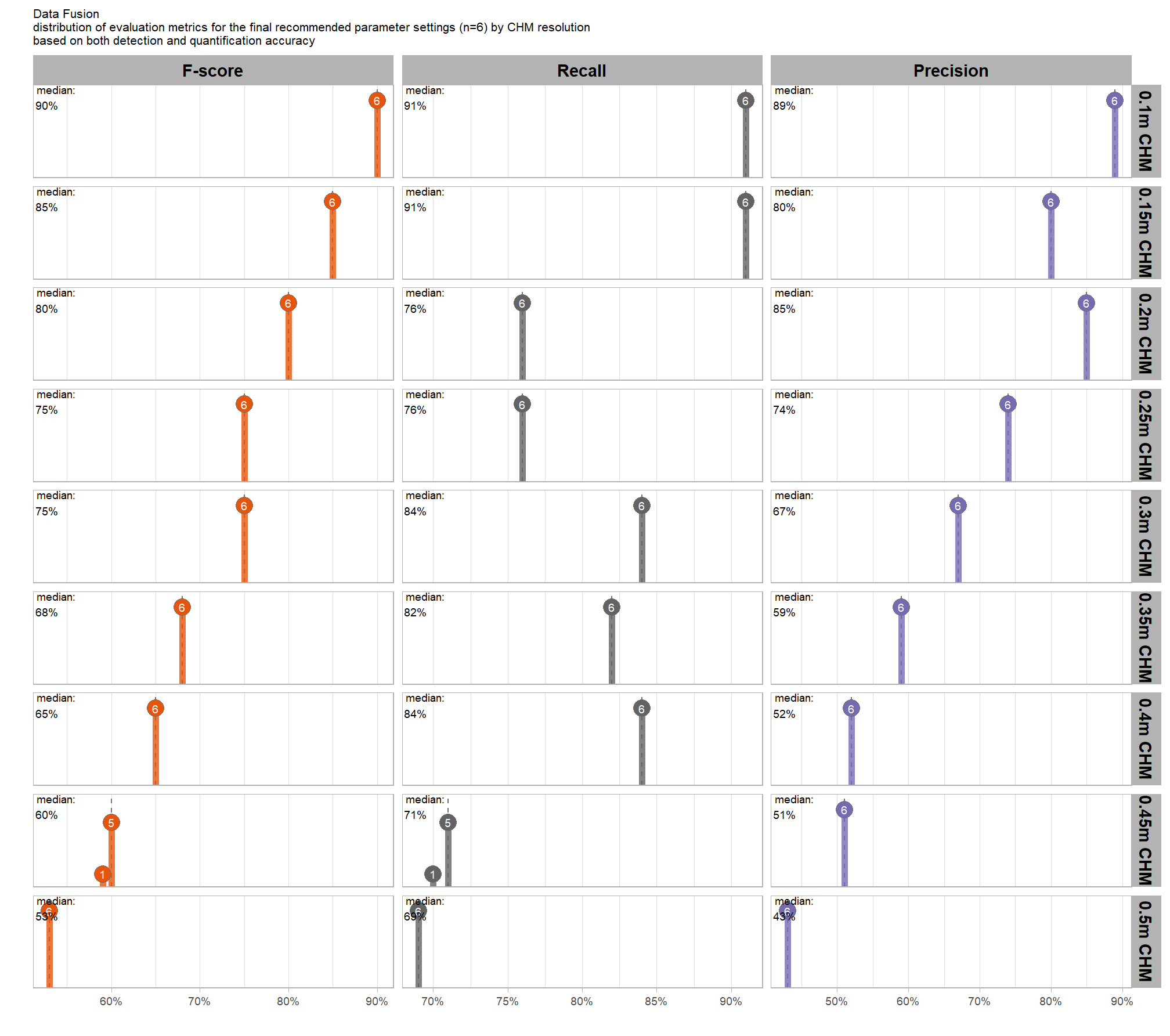
WHAT DID WE LEARN FROM THIS
what is the expected MAPE of the final 6 recommended settings by CHM resolution?
# plot it
plt_form_quantification_dist2(
  df = param_combos_spectral_ranked %>% dplyr::filter(is_final_selection_chm) %>% dplyr::select(!tidyselect::contains("_pct_rank_"))
  , quant_metric = "mape"
  , paste0(
    "Data Fusion"
    , "\ndistribution of pile form quantification metrics for the final recommended parameter settings"
    , " (n="
    , scales::comma(n_th_top_chm,accuracy=1)
    , ") by CHM resolution"
    , "\nbased on both detection and quantification accuracy"
  )
)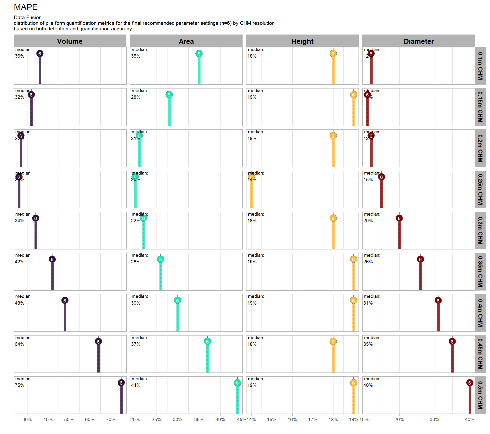
WHAT DID WE LEARN FROM THIS
what is the expected Mean Error (ME) of the final 6 recommended settings by CHM resolution?
# plot it
plt_form_quantification_dist2(
  df = param_combos_spectral_ranked %>% dplyr::filter(is_final_selection_chm) %>% dplyr::select(!tidyselect::contains("_pct_rank_"))
  , quant_metric = "mean"
  , paste0(
    "Data Fusion"
    , "\ndistribution of pile form quantification metrics for the final recommended parameter settings"
    , " (n="
    , scales::comma(n_th_top_chm,accuracy=1)
    , ") by CHM resolution"
    , "\nbased on both detection and quantification accuracy"
  )
)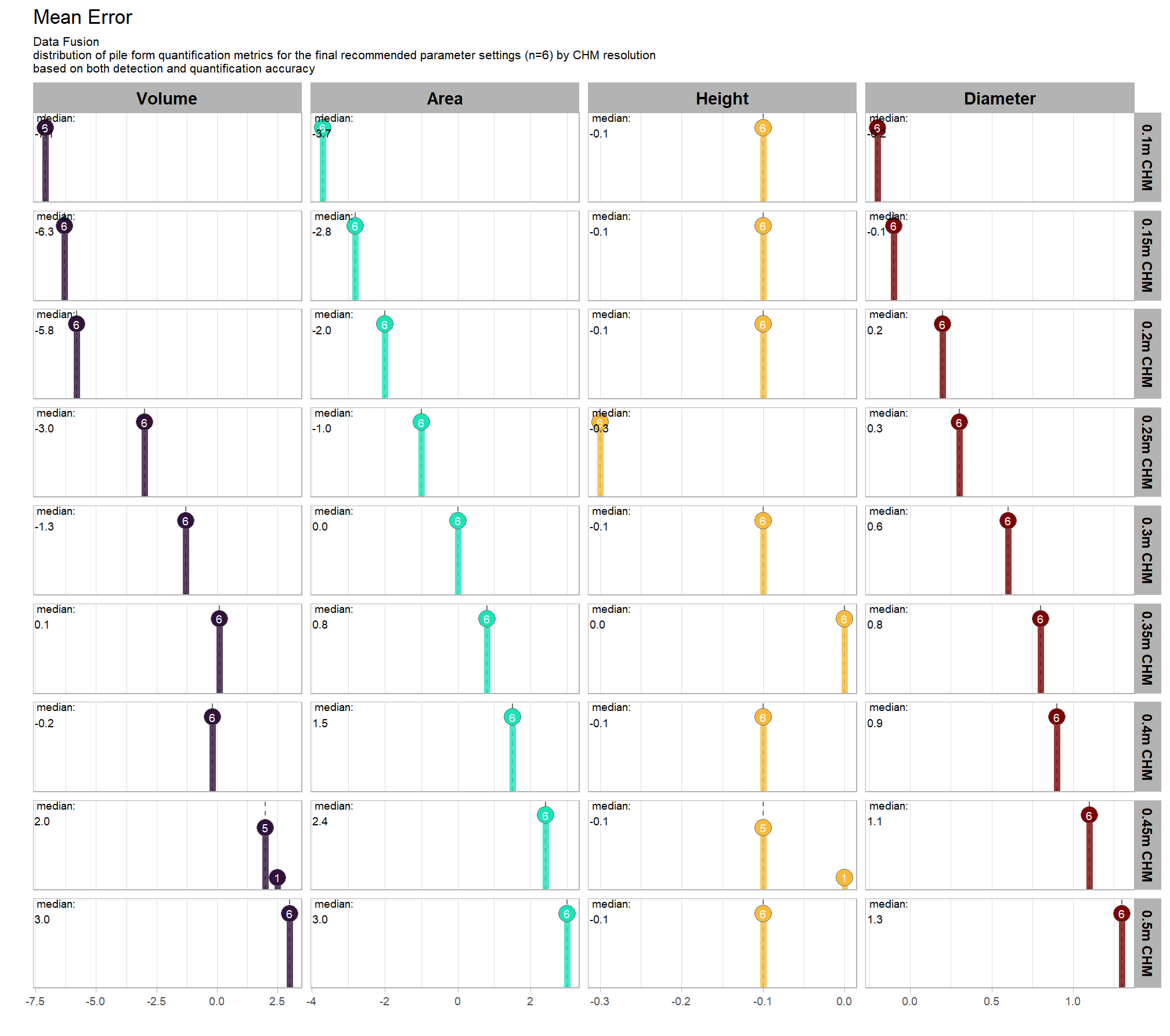
WHAT DID WE LEARN FROM THIS
what is the expected RMSE of the final 6 recommended settings by CHM resolution?
# plot it
plt_form_quantification_dist2(
  df = param_combos_spectral_ranked %>% dplyr::filter(is_final_selection_chm) %>% dplyr::select(!tidyselect::contains("_pct_rank_"))
  , quant_metric = "rmse"
  , paste0(
    "Data Fusion"
    , "\ndistribution of pile form quantification metrics for the final recommended parameter settings"
    , " (n="
    , scales::comma(n_th_top_chm,accuracy=1)
    , ") by CHM resolution"
    , "\nbased on both detection and quantification accuracy"
  )
)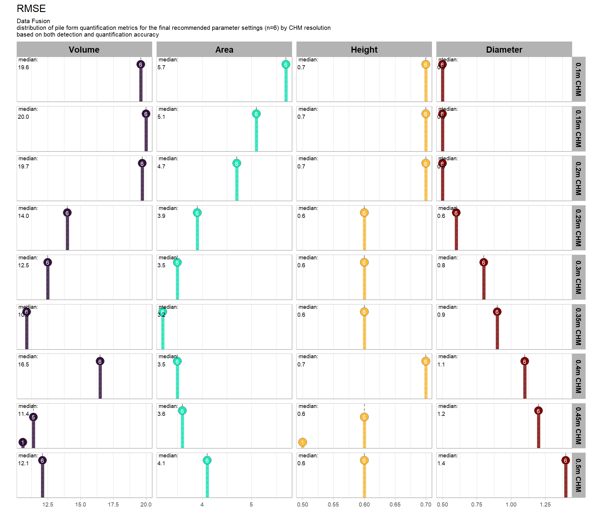
WHAT DID WE LEARN FROM THIS
9.7 Statistical Testing of Hypothoses
using all tested parameter combinations, we’re going build a statistical model to test the following hypotheses about the slash pile detection methodology:
- does CHM resolution influences detection and quantification accuracy?
- does the effect of CHM resolution change based on the inclusion of spectral data versus using only structural data?
- does the use of spectral data have a meaningful impact on detection and quantification accuracy
once the model has been fitted, we can then use it to predict the optimal CHM resolution and other parameter settings for a given approach
the analysis data will include all parameter combinations tested to include all information available for use in the modelling. as such, our analysis data set will be the param_combos_spectral_gt_agg data which includes accuracy measurements at the parameter combination level using both structural only and structural+spectral data. in this data, a row is unique by the full set of parameters tested: max_ht_m, max_area_m2, convexity_pct, circle_fit_iou_pct, chm_res_m, spectral_weight
# convert spectral weight to factor for modelling
param_combos_spectral_gt_agg <- param_combos_spectral_gt_agg %>% dplyr::mutate(spectral_weight = factor(spectral_weight))
# check out this data
param_combos_spectral_gt_agg %>%
  dplyr::select(
    names(param_combos_df), spectral_weight, spectral_weight_fact
    , f_score, precision, recall
    , tidyselect::ends_with("_mape")
  ) %>%
  dplyr::glimpse()
## Rows: 77,466
## Columns: 15
## $ rn <dbl> 1, 2, 3, 4, 5, 6, 7, 8, 9, 10, 11, 12, 13, …
## $ max_ht_m <dbl> 2, 2, 2, 2, 2, 2, 2, 2, 2, 2, 2, 2, 2, 2, 2…
## $ min_area_m2 <dbl> 2, 2, 2, 2, 2, 2, 2, 2, 2, 2, 2, 2, 2, 2, 2…
## $ max_area_m2 <dbl> 10, 10, 10, 10, 10, 10, 10, 10, 10, 10, 10,…
## $ convexity_pct <dbl> 0.3, 0.3, 0.3, 0.3, 0.3, 0.3, 0.4, 0.4, 0.4…
## $ circle_fit_iou_pct <dbl> 0.3, 0.4, 0.5, 0.6, 0.7, 0.8, 0.3, 0.4, 0.5…
## $ spectral_weight <fct> 1, 1, 1, 1, 1, 1, 1, 1, 1, 1, 1, 1, 1, 1, 1…
## $ spectral_weight_fact <fct> structural+spectral, structural+spectral, s…
## $ f_score <dbl> 0.7874016, 0.8200837, 0.8384279, 0.8396226,…
## $ precision <dbl> 0.7518797, 0.8305085, 0.8888889, 0.9780220,…
## $ recall <dbl> 0.8264463, 0.8099174, 0.7933884, 0.7355372,…
## $ pct_diff_area_field_mape <dbl> 0.3508412, 0.3491516, 0.3494401, 0.3469688,…
## $ pct_diff_diameter_mape <dbl> 0.1253545, 0.1257875, 0.1264195, 0.1283161,…
## $ pct_diff_height_mape <dbl> 0.1153659, 0.1167828, 0.1179042, 0.1191909,…
## $ pct_diff_volume_field_mape <dbl> 0.3535689, 0.3529049, 0.3543701, 0.3547730,…a row is unique by the full set of parameters tested: max_ht_m, max_area_m2, convexity_pct, circle_fit_iou_pct, chm_res_m, spectral_weight
# a row is unique by max_ht_m, max_area_m2, convexity_pct, circle_fit_iou_pct, chm_res_m, and spectral_weight
identical(
  param_combos_spectral_gt_agg %>% dplyr::distinct(max_ht_m, max_area_m2, convexity_pct, circle_fit_iou_pct, chm_res_m, spectral_weight) %>% nrow()
  , param_combos_spectral_gt_agg %>% nrow()
)
## [1] TRUEhere are the number of records which returned valid predicted slash pile polygons by CHM resolution and data input setting (i.e. structural only versus data fusion). the number of records for the data fusion approach (“structural+spectral”) should be roughly five times the number of records as the structural only approach because we tested five different settings of the structural_weight parameter from the lowest weighting of the spectral data of “1” (only one spectral index threshold must be met) to the highest weighting of spectral data “5” (all spectral index thresholds must be met)
param_combos_spectral_gt_agg %>%
  dplyr::count(chm_res_m_desc,spectral_weight_fact) %>%
  ggplot2::ggplot(mapping = ggplot2::aes(x=n,y=spectral_weight_fact, color = spectral_weight_fact, fill = spectral_weight_fact)) +
    ggplot2::geom_col(width = 0.6) +
    ggplot2::geom_text(
      mapping = ggplot2::aes(label=scales::comma(n))
      , color = "black", size = 3
      , hjust = -0.1
    ) +
    ggplot2::facet_grid(rows = dplyr::vars(chm_res_m_desc)) +
    harrypotter::scale_fill_hp_d(option = "slytherin") +
    harrypotter::scale_color_hp_d(option = "slytherin") +
    ggplot2::scale_x_continuous(labels = scales::comma, expand = ggplot2::expansion(mult = c(0,.1))) +
    ggplot2::labs(y="") +
    ggplot2::theme_light() +
    ggplot2::theme(
      legend.position = "none"
      , strip.text.y = ggplot2::element_text(size = 9, color = "black", face = "bold")
    )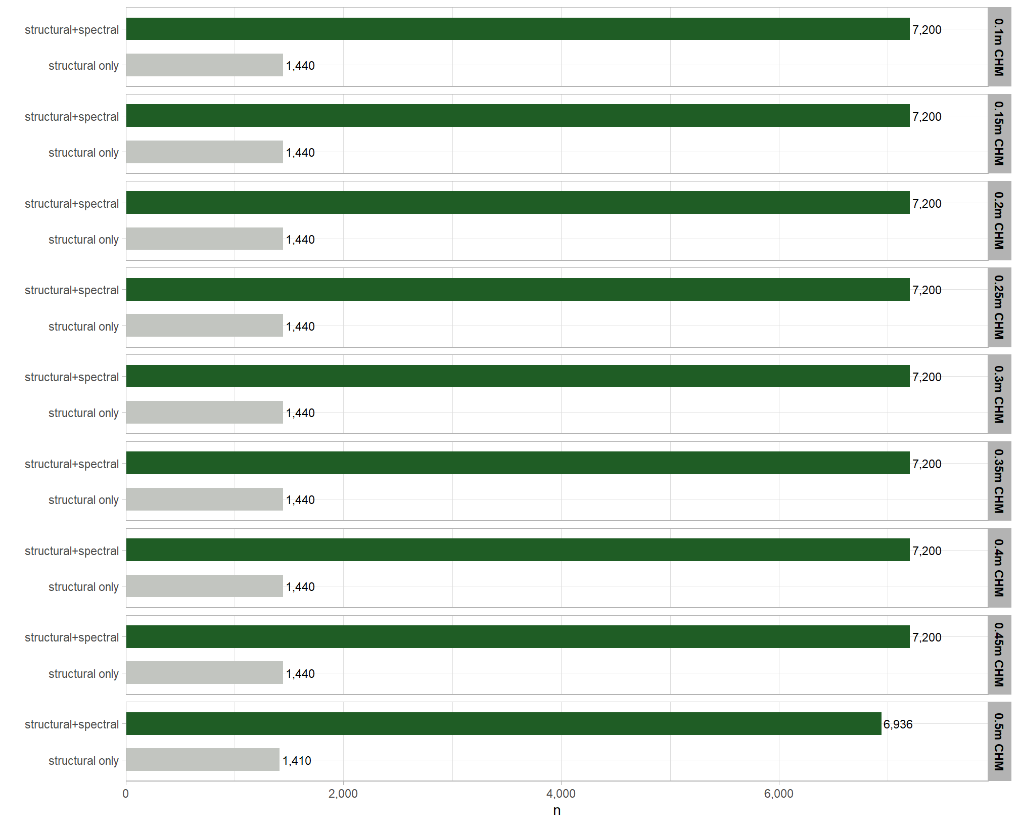
9.7.1 Bayesian generalized linear model (GLM)
given that our data contains only one observation per parameter combination, we’re going to use a Bayesian Beta regression model to ensure a statistically sound approach and interpretable relationships between each parameter and the dependent variable (e.g. F-score). our model will treat the parameters as a mix of continuous and nominal variables, preventing model saturation (where the model has as many parameters to estimate as data points, so the data perfectly explains the model). A Bayesian hierarchical model would not be appropriate for this structure, since it is designed for datasets with nested or grouped observations (e.g. if we had evaluated the method across different plots or study sites).
Our Bayesian Beta regression models the F-score with a Beta distribution because it is a proportion between 0 and 1, which ensures that the predictions and uncertainty estimates are always within the valid range. We’re treating the four structural parameters (e.g. max_ht_m and circle_fit_iou_pct) and the CHM resolution (chm_res_m) as metric (i.e., continuous) variables, as this is statistically sound for our data and allows for a continuous interpretation where the model coefficient will represent the change in F-score for a one-unit change in the parameter value. The spectral_weight parameter, however, will be treated as nominal to capture its discrete effects without assuming a linear relationship. Finally, we’ll include an interaction between chm_res_m and spectral_weight to directly compare the effect of CHM resolution with and without the use of spectral data.
we’ll generally follow Kurz (2023a; 2023b; 2025 for multiple linear regression model building using the brms Bayesian model framework based on McElreath (2015, Ch. 5,7) and Kruschke (2015, Ch. 18)
the fully factored Bayesian statistical model that details the likelihood, linear model, and priors used is:
\[\begin{align*} \text{F-score}_i \sim & \operatorname{Beta}(\mu_{i}, \phi) \\ \operatorname{logit}(\mu_i) = & \beta_0 \\ & + \beta_1 \cdot \text{max_ht_m}_i + \beta_2 \cdot \text{max_area_m2}_i \\ & + \beta_3 \cdot \text{convexity_pct}_i + \\ & + \beta_4 \cdot \text{circle_fit_iou_pct}_i + \beta_5 \cdot \text{circle_fit_iou_pct}^{2}_{i} \\ & + \beta_6 \cdot \text{chm_res_m}_i \\ & + \beta_7 \cdot \text{spectral_weight}_{i,1} + \dots + \beta_{11} \cdot \text{spectral_weight}_{i,5} \\ & + \beta_{12} \cdot \text{chm_res_m}_i \cdot \text{spectral_weight}_{i,1} + \dots + \beta_{16} \cdot \text{chm_res_m}_i \cdot \text{spectral_weight}_{i,5} \\ \beta_j \sim & \operatorname{Normal}(0, \sigma_j) \quad \text{for } j = 0, \dots, 16 \\ \sigma_j \sim & \operatorname{Student T}(3,0,2.5) \quad \text{for } j = 0, \dots, 16 \\ \phi \sim & \operatorname{Gamma}(0.01,0.01) \\ \end{align*}\]
where, \(i\) represents a single observation in the dataset which corresponds to a specific combination of the six parameters (, max_ht_m, max_area_m2, convexity_pct, circle_fit_iou_pct, chm_res_m, and spectral_weight) and its resulting F-score. and j is used to index the different beta coefficients, which correspond to the intercept and the effects of each of the independent variables and their interactions.
prior to building the model let’s check out the correlations between our predictor variables to make sure we properly captured the relationships between the parameters
let’s fit the model using the brms framework to fit Bayesian regression models using the Stan probabilistic programming language. if we want to set the prior for \(\beta_0\) given a non-centered predictors, then we need to use the 0 + Intercept syntax to fit the model (see Kurz 2025 for full discussion), but we’ll just fit the model with the brsm::brm() default settings which automatically mean centers the predictors and also set the intercept to 0 so that we get explicit coefficient estimates for each level of our spectral_weight nominal variable which determines the intercept in this model
brms_f_score_mod <- brms::brm(
  formula = f_score ~
    # 0 + Intercept + ## to set prior for b0
    # 1 + # not setting prior for b0
    0 + # no intercept to allow all values of spectral_weight to be shown instead of set as the baseline
    max_ht_m + max_area_m2 + convexity_pct +
    circle_fit_iou_pct + I(circle_fit_iou_pct^2) +
    chm_res_m + spectral_weight + chm_res_m:spectral_weight
  , data = param_combos_spectral_gt_agg %>% dplyr::slice_sample(prop = 0.2)
  , family = Beta(link = "logit")
  # , prior = c(
  #   brms::prior(student_t(3, 0, 5), class = "b")
  #   , brms::prior(gamma(0.01, 0.01), class = "phi")
  # )
  # mcmc
  , iter = 20000, warmup = 10000
  , chains = 4
  # , control = list(adapt_delta = 0.999, max_treedepth = 13)
  , cores = lasR::half_cores()
  , file = paste0("../data/", "brms_f_score_mod")
)
# brms::make_stancode(brms_f_score_mod)
# brms::prior_summary(brms_f_score_mod)
# print(brms_f_score_mod)
# brms::neff_ratio(brms_f_score_mod)
# brms::rhat(brms_f_score_mod)
# brms::nuts_params(brms_f_score_mod)
The brms::brm model summary
brms_f_score_mod %>%
  brms::posterior_summary() %>%
  as.data.frame() %>%
  tibble::rownames_to_column(var = "parameter") %>%
  dplyr::rename_with(tolower) %>%
  dplyr::filter(
    stringr::str_starts(parameter, "b_")
    | parameter == "phi"
  ) %>%
  dplyr::mutate(
    dplyr::across(
      dplyr::where(is.numeric)
      , ~ dplyr::case_when(
        stringr::str_ends(parameter,"_pct") ~ .x*0.01 # convert to percentage point change
        , T ~ .x
      )
    )
  ) %>%
  kableExtra::kbl(digits = 3, caption = "Bayesian model for F-score") %>%
kableExtra::kable_styling()| parameter | estimate | est.error | q2.5 | q97.5 |
|---|---|---|---|---|
| b_max_ht_m | -0.028 | 0.002 | -0.033 | -0.023 |
| b_max_area_m2 | 0.003 | 0.000 | 0.002 | 0.003 |
| b_convexity_pct | 0.000 | 0.000 | 0.000 | 0.001 |
| b_circle_fit_iou_pct | 0.175 | 0.001 | 0.172 | 0.177 |
| b_Icircle_fit_iou_pctE2 | -18.193 | 0.114 | -18.417 | -17.973 |
| b_chm_res_m | -4.229 | 0.053 | -4.334 | -4.125 |
| b_spectral_weight0 | -2.483 | 0.038 | -2.558 | -2.409 |
| b_spectral_weight1 | -2.477 | 0.039 | -2.553 | -2.403 |
| b_spectral_weight2 | -2.488 | 0.039 | -2.564 | -2.413 |
| b_spectral_weight3 | -2.419 | 0.038 | -2.494 | -2.345 |
| b_spectral_weight4 | -1.956 | 0.038 | -2.032 | -1.881 |
| b_spectral_weight5 | -2.777 | 0.038 | -2.853 | -2.703 |
| b_chm_res_m:spectral_weight1 | -0.055 | 0.077 | -0.205 | 0.097 |
| b_chm_res_m:spectral_weight2 | -0.030 | 0.076 | -0.178 | 0.121 |
| b_chm_res_m:spectral_weight3 | -0.122 | 0.075 | -0.269 | 0.026 |
| b_chm_res_m:spectral_weight4 | -0.691 | 0.076 | -0.841 | -0.541 |
| b_chm_res_m:spectral_weight5 | 1.556 | 0.074 | 1.409 | 1.700 |
| phi | 22.146 | 0.194 | 21.772 | 22.525 |
note the quadratic coefficient, Kruschke (2015) provides some insight on how to interpret:
A quadratic has the form \(y = \beta_{0} + \beta_{1}x + \beta_{2}x2\). When \(\beta_{2}\) is zero, the form reduces to a line. Therefore, this extended model can produce any fit that the linear model can. When \(\beta_{2}\) is positive, a plot of the curve is a parabola that opens upward. When \(\beta_{2}\) is negative, the curve is a parabola that opens downward. We have no reason to think that the curvature in the family-income data is exactly a parabola, but the quadratic trend might describe the data much better than a line alone. (p. 496)
9.7.1.1 Posterior Predictive Checks
Markov chain Monte Carlo (MCMC) simulations were conducted using the brms package (Bürkner 2017) to estimate posterior predictive distributions of the parameters of interest. We ran xxx chains of xxx iterations with the first xxx discarded as burn-in. Trace-plots were utilized to visually assess model convergence.
check the trace plots for problems with convergence of the Markov chains
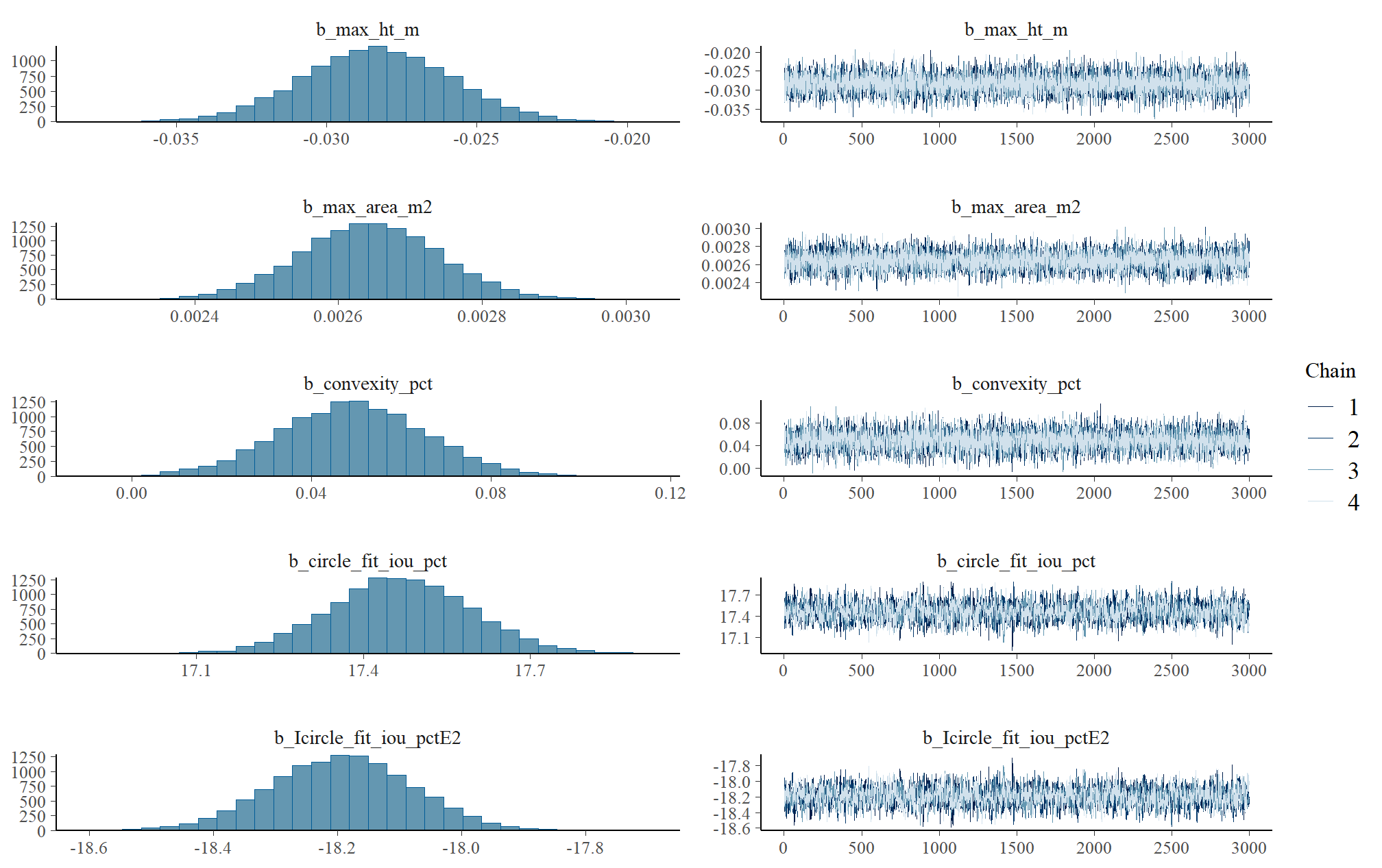
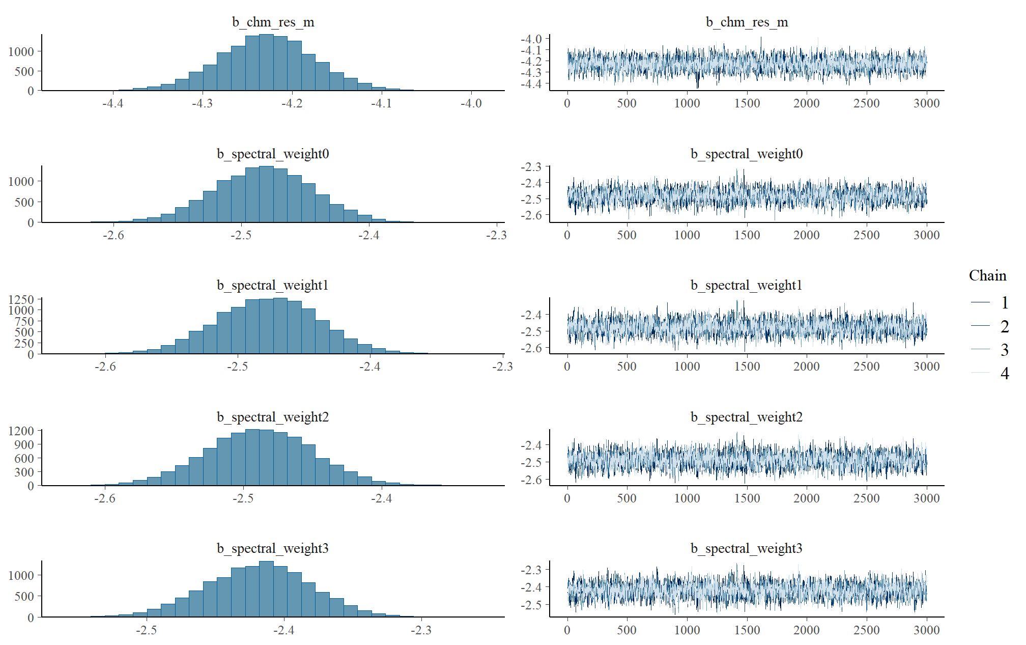
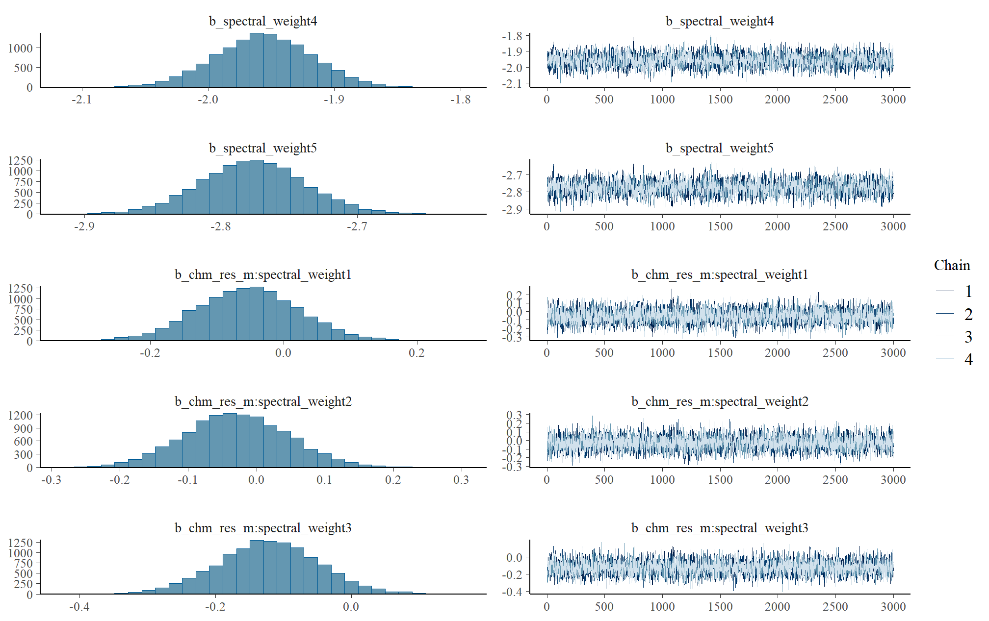
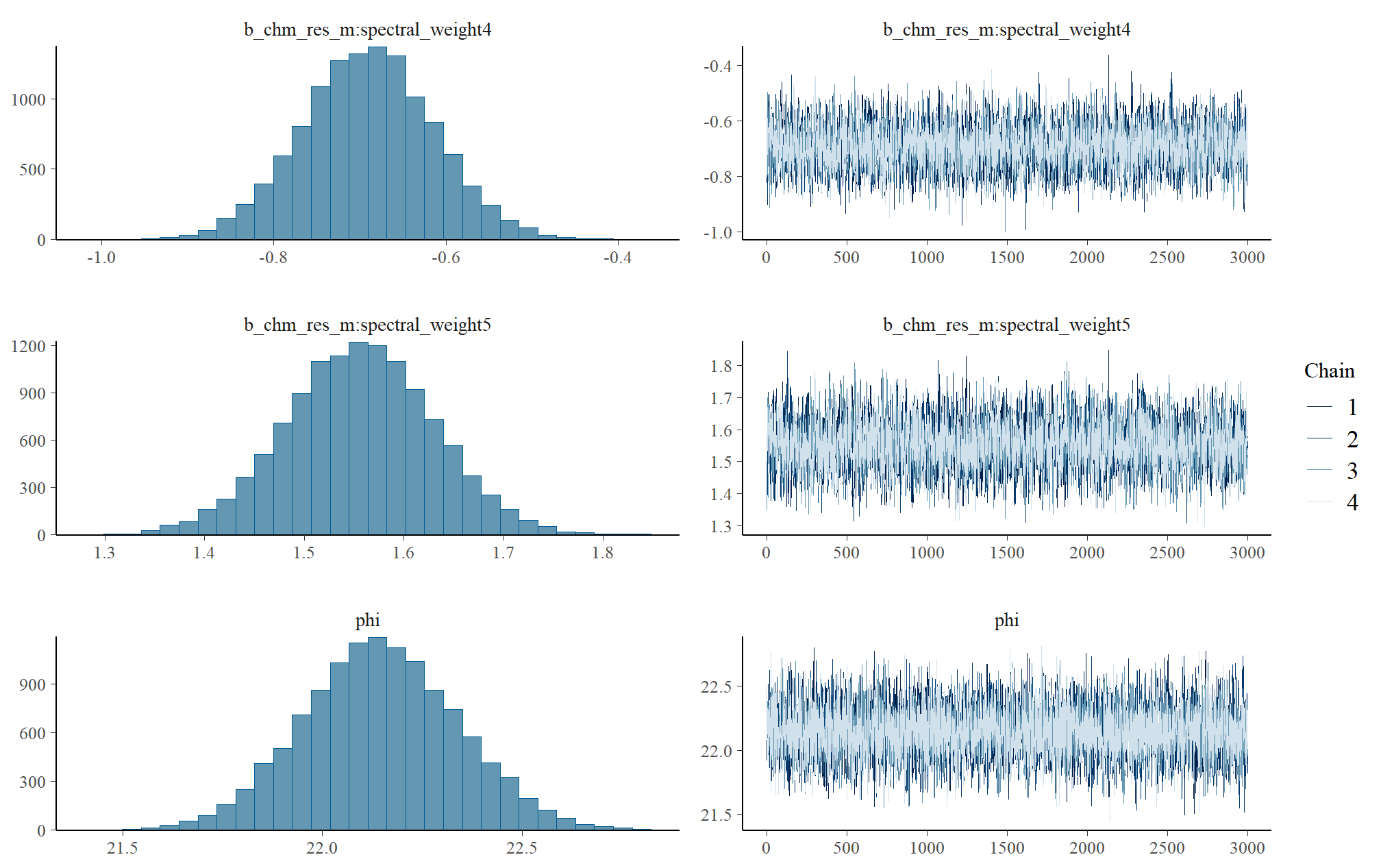
Sufficient convergence was checked with \(\hat{R}\) values near 1 (Brooks & Gelman, 1998).
check our \(\hat{R}\) values
brms::mcmc_plot(brms_f_score_mod, type = "rhat_hist") +
  ggplot2::scale_x_continuous(breaks = scales::breaks_extended(n = 6)) +
  ggplot2::theme_light() +
  ggplot2::theme(
    legend.position = "top", legend.direction = "horizontal"
  )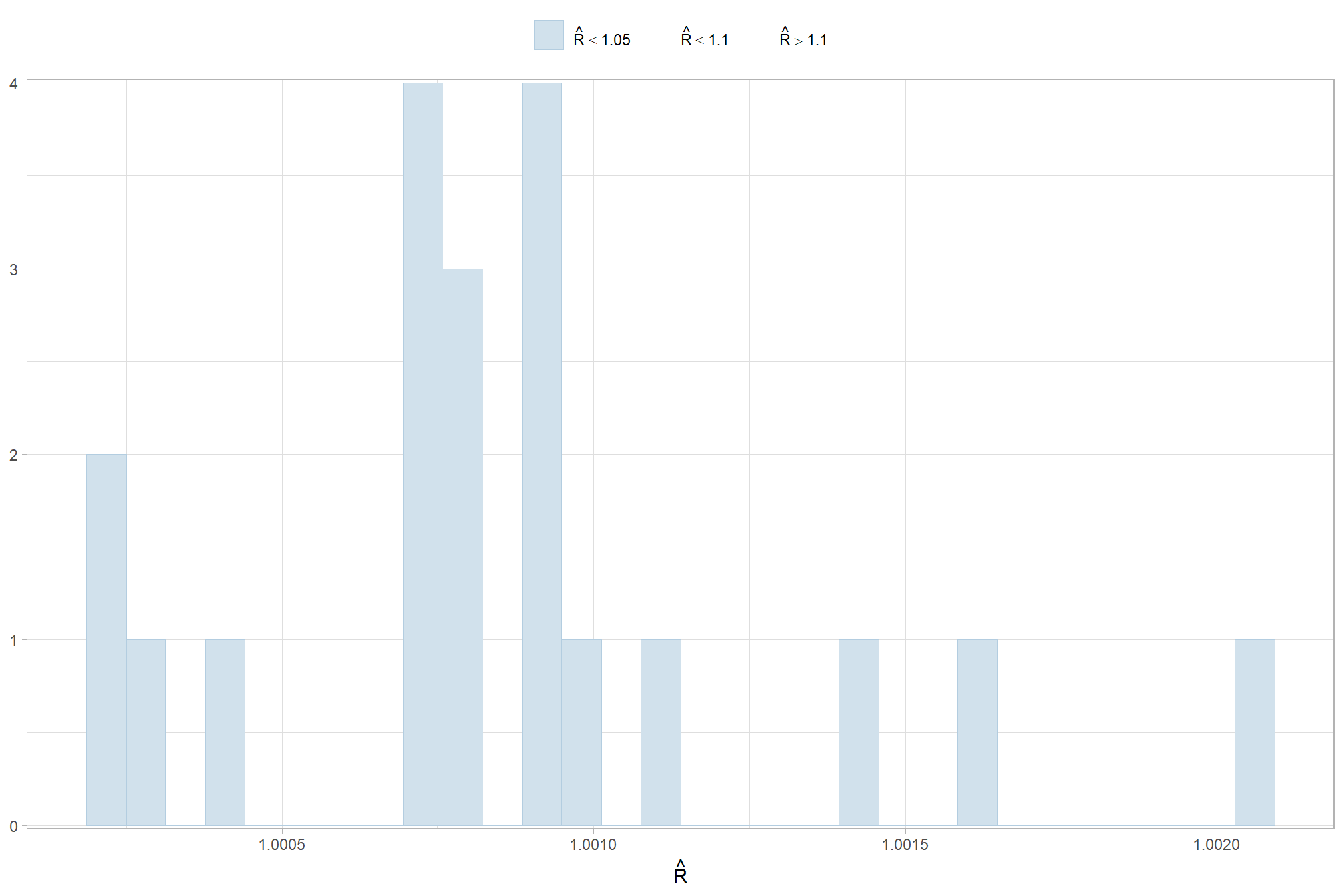
The effective length of an MCMC chain is indicated by the effective sample size (ESS), which refers to the sample size of the MCMC chain not to the sample size of the data Kruschke (2015) notes:
One simple guideline is this: For reasonably accurate and stable estimates of the limits of the 95% HDI, an ESS of 10,000 is recommended. This is merely a heuristic based on experience with practical applications, it is not a requirement. If accuracy of the HDI limits is not crucial for your application, then a smaller ESS may be sufficient. (p.184)
# get ess values from model summary
summary(brms_f_score_mod) %>%
  purrr::pluck("fixed") %>%
  dplyr::as_tibble() %>%
  dplyr::rename(ess = Bulk_ESS) %>%
  dplyr::mutate(parameter = dplyr::row_number(), chk = ess<10000) %>%
  ggplot2::ggplot(ggplot2::aes(x = ess, y = parameter, color = chk, fill = chk)) +
  ggplot2::geom_vline(xintercept = 10000, linetype = "dashed", color = "gray44", lwd = 1.2) +
  ggplot2::geom_segment( ggplot2::aes(x = 0, xend=ess, yend=parameter), color="black") +
  ggplot2::geom_point() +
  ggplot2::scale_fill_manual(values = c("red3", "blue3")) +
  ggplot2::scale_color_manual(values = c("red3", "blue3")) +
  ggplot2::scale_y_continuous(NULL, breaks = NULL) +
  ggplot2::scale_x_continuous(labels = scales::comma) +
  ggplot2::labs(
    x = "ESS"
    , subtitle = "MCMC chain resolution check for effective sample size (ESS) values"
    , y = ""
    , title = "F-Score"
  ) +
  ggplot2::theme_light() +
  ggplot2::theme(
    legend.position = "none"
    , axis.text.y = ggplot2::element_text(size = 4)
    , panel.grid.major.x = ggplot2::element_blank()
    , panel.grid.minor.x = ggplot2::element_blank()
    , plot.subtitle = ggplot2::element_text(size = 8)
    , plot.title = ggplot2::element_text(size = 9)
  )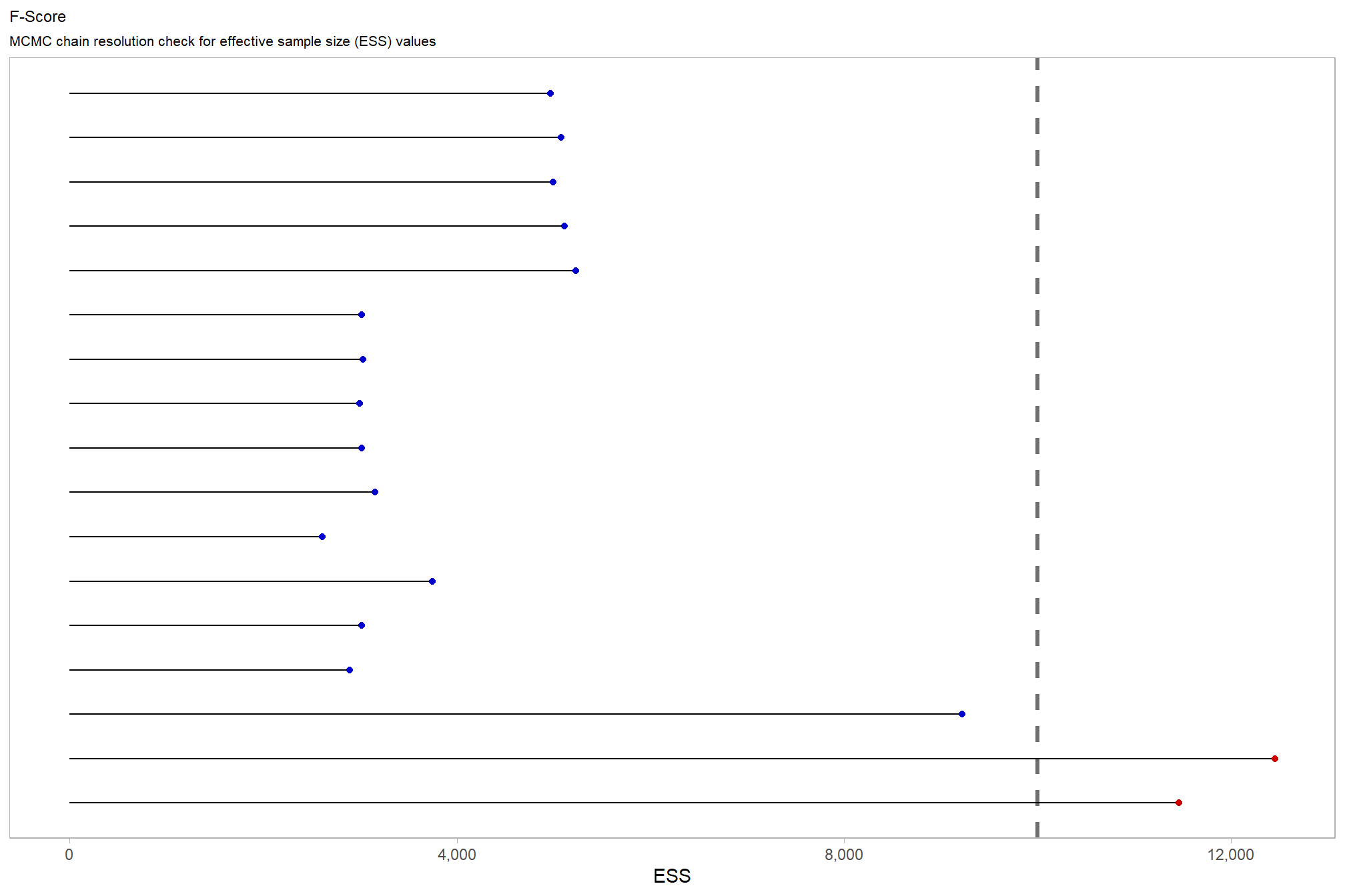
# # and another effective sample size check
# brms::mcmc_plot(brms_f_score_mod, type = "neff_hist") +
#   theme_light() +
#   theme(
#     legend.position = "top", legend.direction = "horizontal"
#   )
Posterior predictive checks were used to evaluate model goodness-of-fit by comparing data simulated from the model with the observed data used to estimate the model parameters (Hobbs & Hooten, 2015). Calculating the proportion of MCMC iterations in which the test statistic (i.e., mean and sum of squares) from the simulated data and observed data are more extreme than one another provides the Bayesian p-value. Lack of fit is indicated by a value close to 0 or 1 while a value of 0.5 indicates perfect fit (Hobbs & Hooten, 2015).
To learn more about this approach to posterior predictive checks, check out Gabry’s (2022) vignette, Graphical posterior predictive checks using the bayesplot package.
posterior-predictive check to make sure the model does an okay job simulating data that resemble the sample data
# posterior predictive check
brms::pp_check(
    brms_f_score_mod
    , type = "dens_overlay"
    , ndraws = 100
  ) +
  ggplot2::labs(subtitle = "posterior-predictive check (overlaid densities)") +
  ggplot2::theme_light() +
  ggplot2::scale_y_continuous(NULL, breaks = NULL) +
  ggplot2::theme(
    legend.position = "top", legend.direction = "horizontal"
    , legend.text = ggplot2::element_text(size = 14)
    , plot.subtitle = ggplot2::element_text(size = 8)
    , plot.title = ggplot2::element_text(size = 9)
  )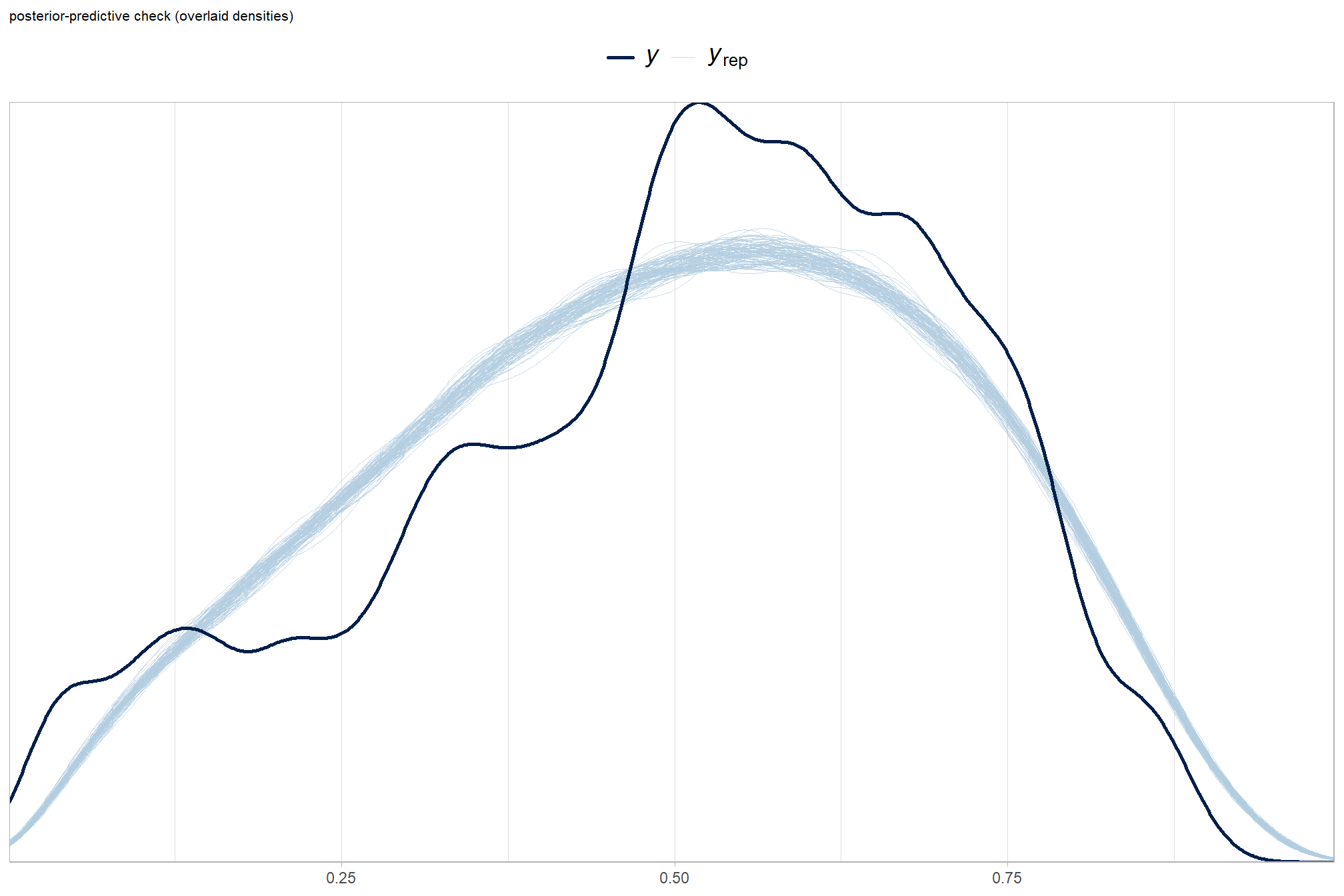
another way
brms::pp_check(brms_f_score_mod, type = "ecdf_overlay", ndraws = 100) +
  ggplot2::labs(subtitle = "posterior-predictive check (ECDF: empirical cumulative distribution function)") +
  ggplot2::theme_light() +
  ggplot2::theme(
    legend.position = "top", legend.direction = "horizontal"
    , legend.text = ggplot2::element_text(size = 14)
  )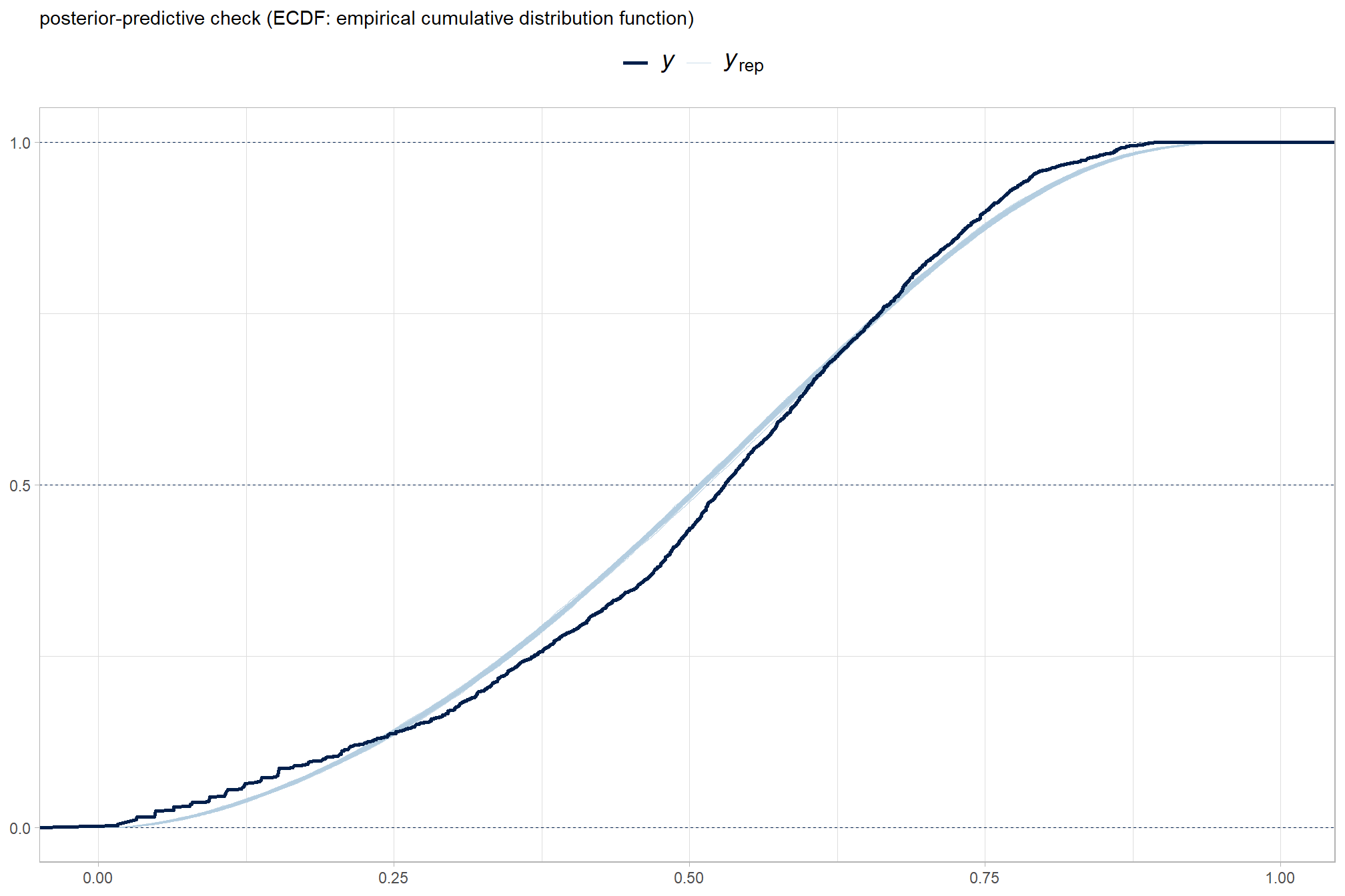
and another posterior predictive check for the overall model combining mean and sd
brms::pp_check(brms_f_score_mod, type = "stat_2d", ndraws = 888) +
  ggplot2::theme_light() +
  ggplot2::labs(title = "F-Score") +
  ggplot2::theme(
    legend.position = "top", legend.direction = "horizontal"
    , legend.text = ggplot2::element_text(size = 8)
    , plot.title = ggplot2::element_text(size = 9)
  )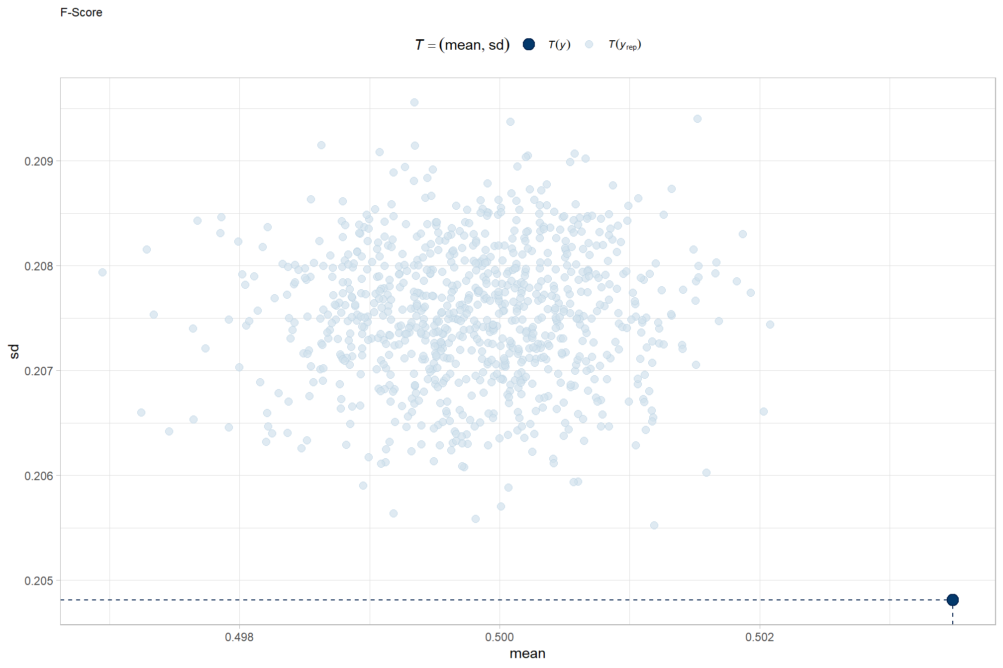
9.7.2 Conditional Effects
let’s check for the main effects of the individual variables on F-score (averages across all other effects)
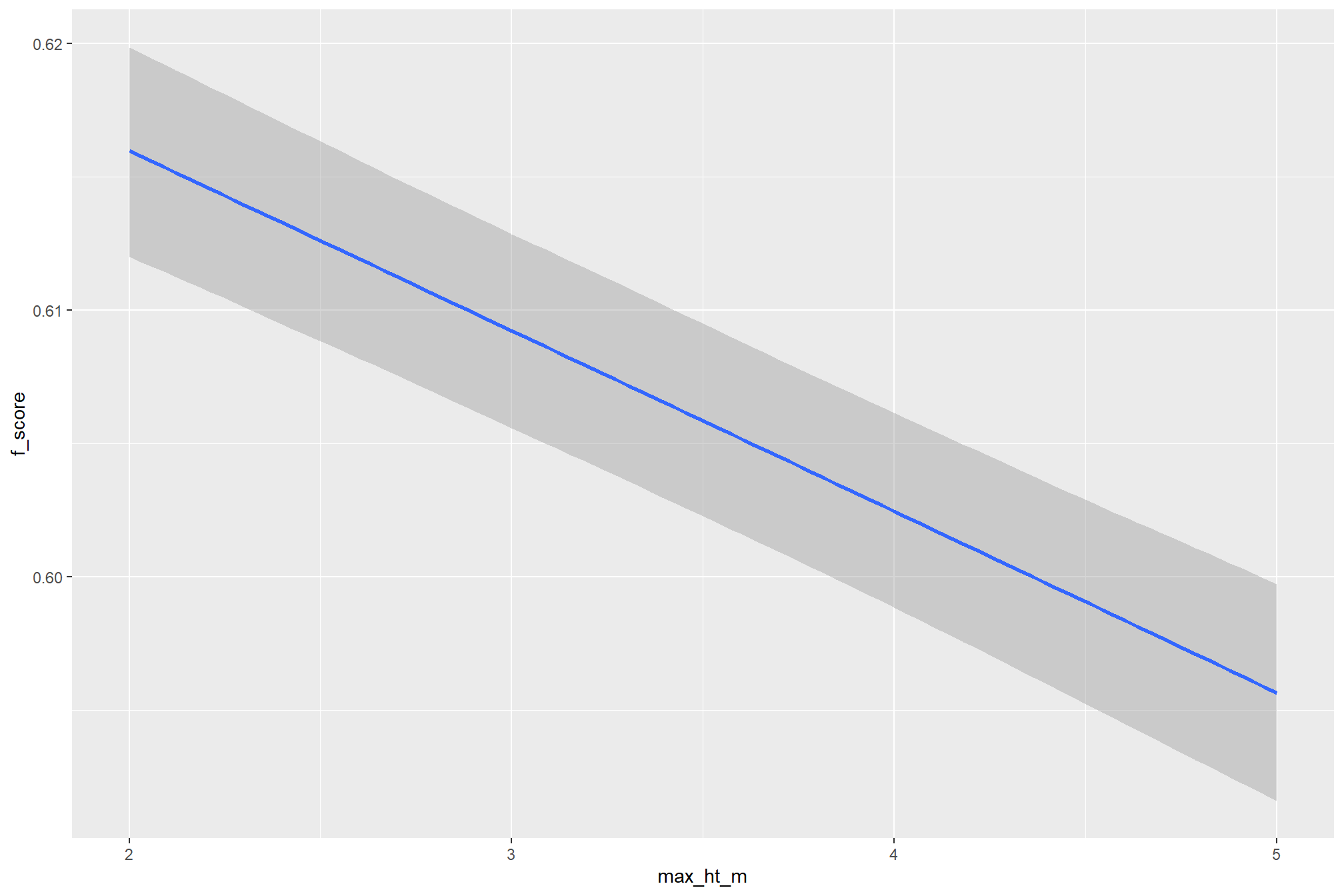
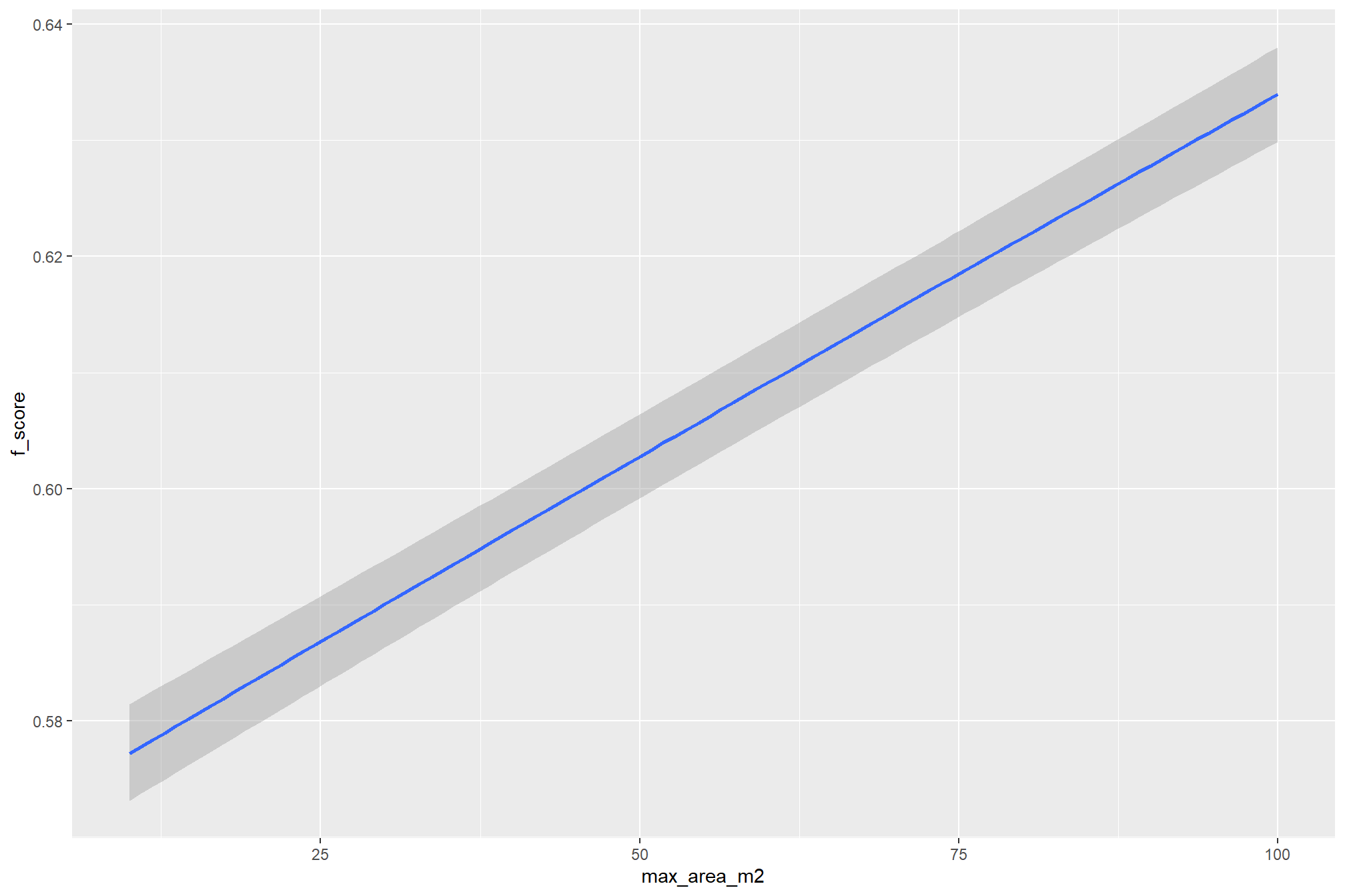
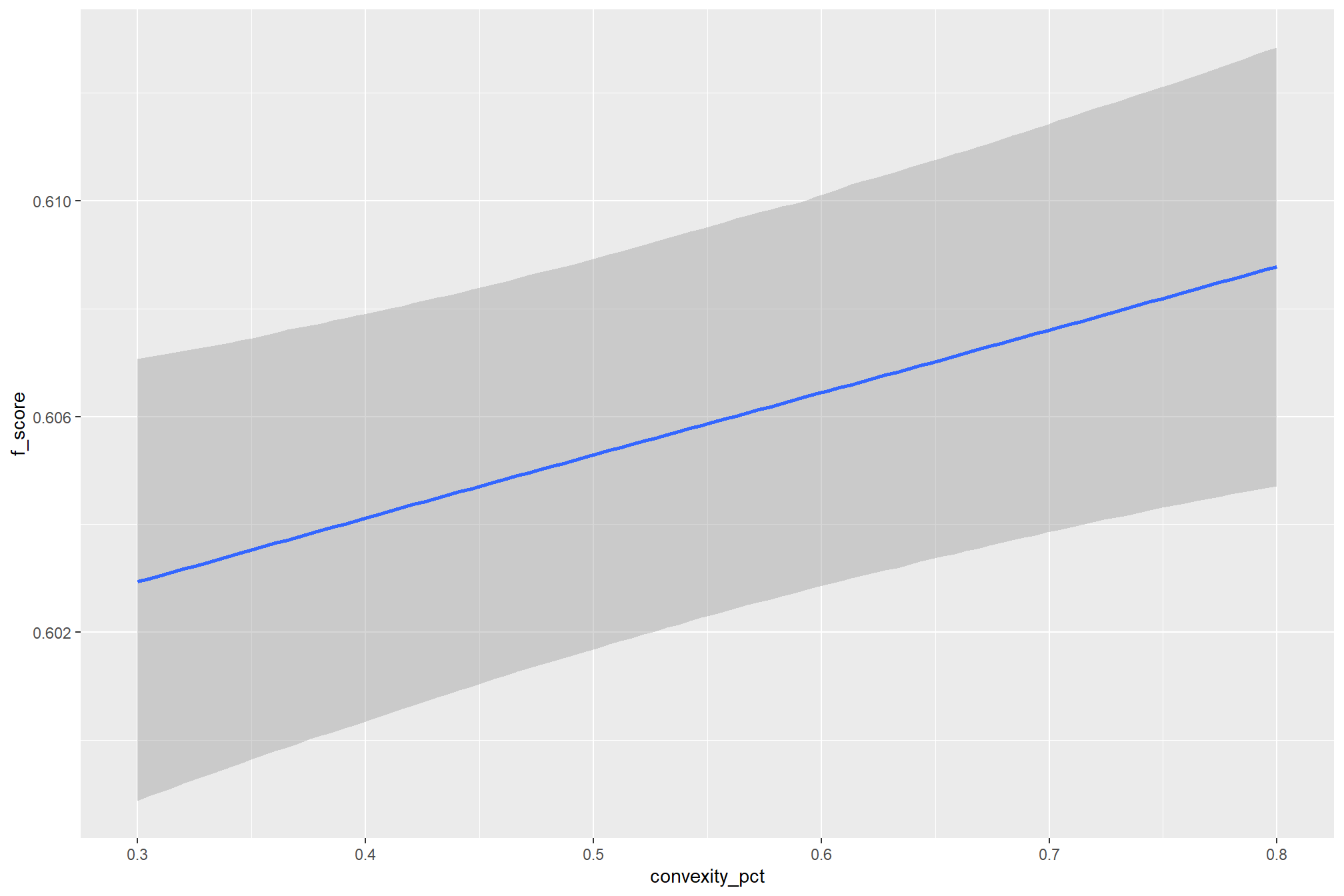
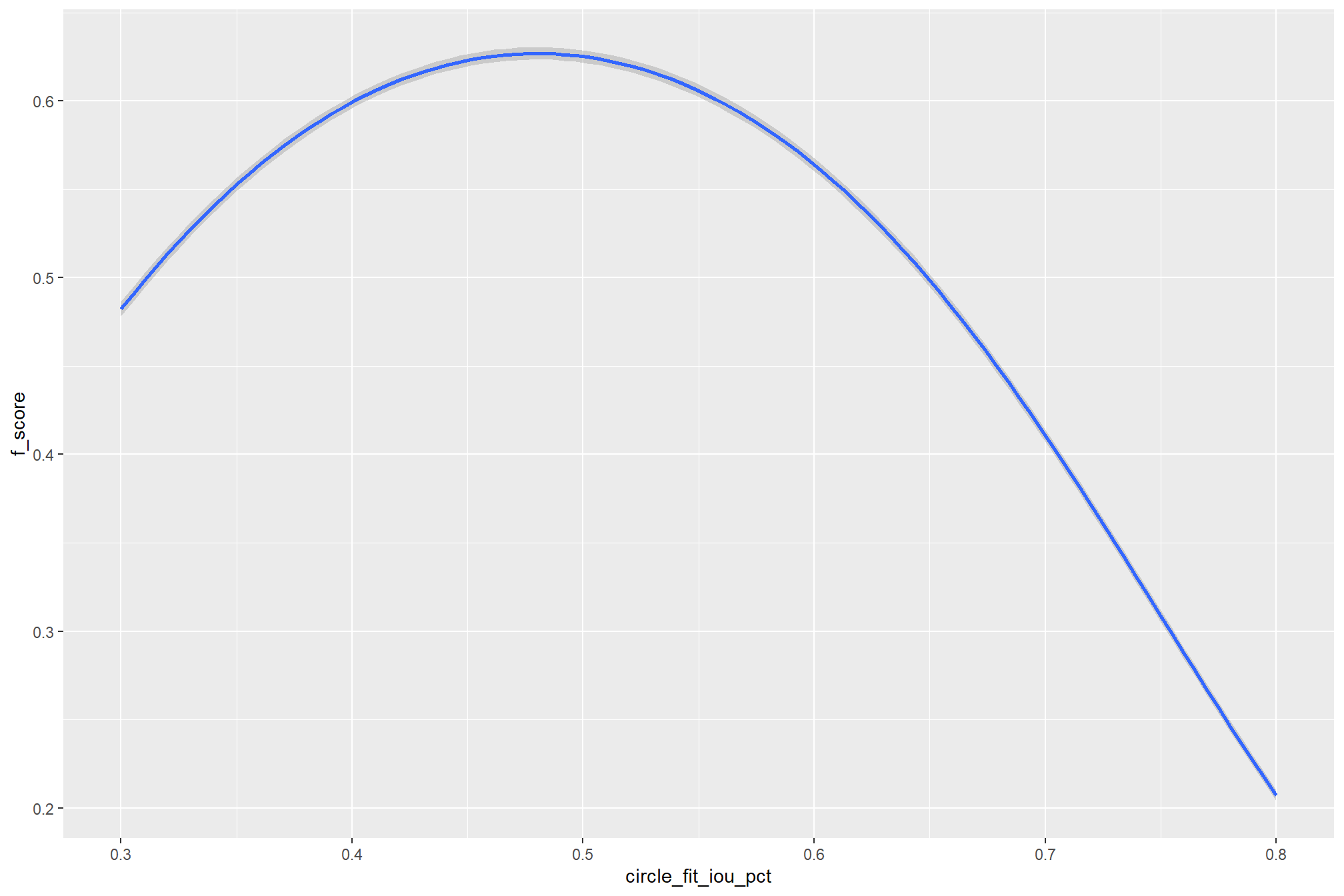
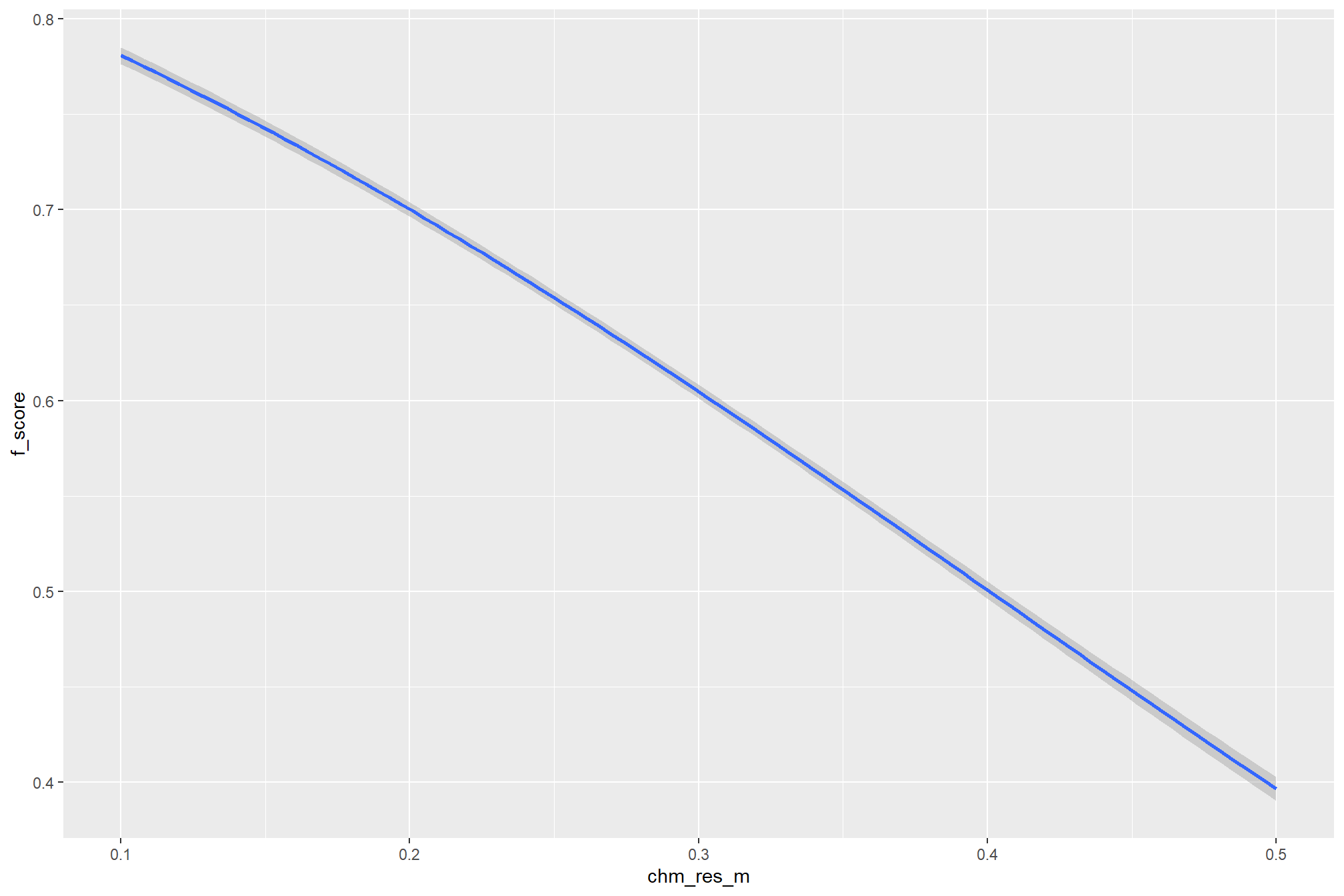
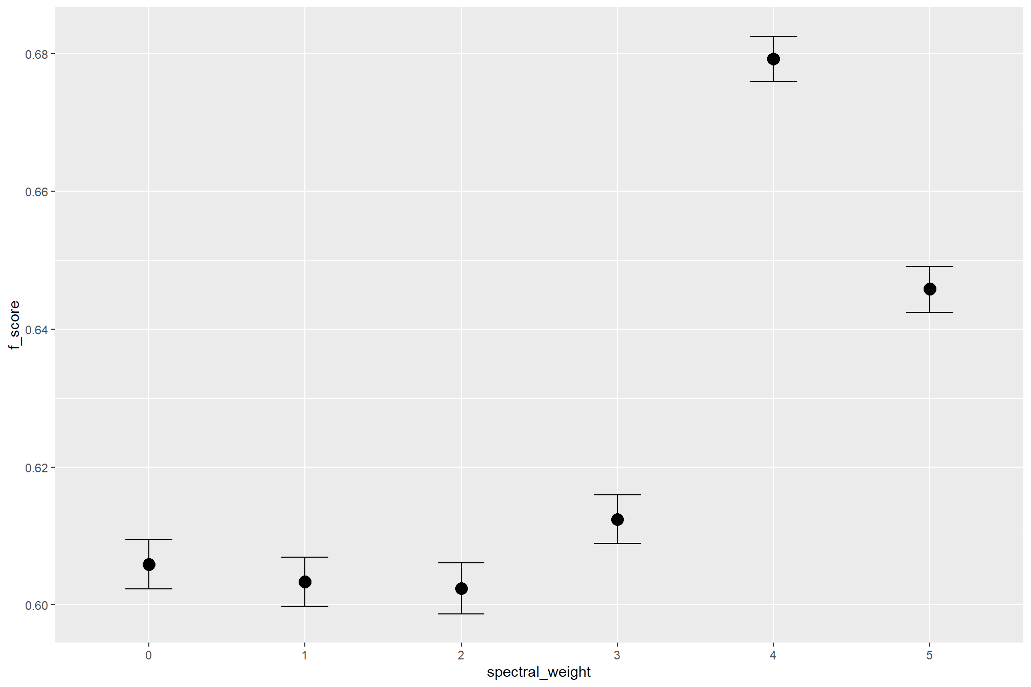
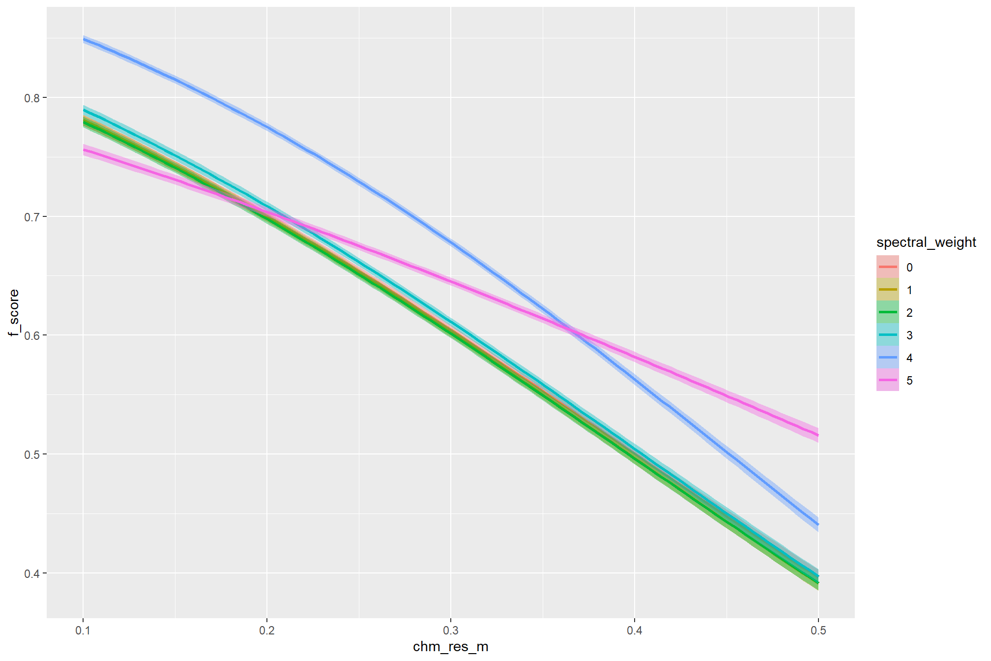
### ggplot version
# brms::conditional_effects(brms_f_score_mod) %>%
#   purrr::pluck("max_ht_m") %>%
#   ggplot(aes(x = max_ht_m)) +
#   geom_ribbon(aes(ymin = lower__, ymax = upper__), fill = "blue", alpha = 0.2) +
#   geom_line(aes(y = estimate__), color = "blue") +
#   labs(
#     x = "max_ht_m",
#     y = "F-score",
#     title = "Conditional Effects"
#   )
and we can test if the structural parameter settings (e.g. model coefficients) have a non-zero impact on F-score
# easy way to get the default coeff plot
# brms::mcmc_plot(brms_f_score_mod)
# custom coeff plot
struct_draws_temp <-
  brms::as_draws_df(brms_f_score_mod) %>%
  # dplyr::select(b_circle_fit_iou_pct) %>% ggplot(aes(x=b_circle_fit_iou_pct)) + tidybayes::stat_halfeye()
  dplyr::select(tidyselect::starts_with("b_")) %>%
  tidyr::pivot_longer(dplyr::everything()) %>%
  dplyr::mutate(
    name = stringr::str_remove(name, "\\bb_") %>%
      stringr::str_remove("\\bI")
  ) %>%
  dplyr::filter(
    name %in% c("max_ht_m" , "max_area_m2" , "convexity_pct" , "circle_fit_iou_pct" )
    | stringr::str_ends(name,"E2")
  ) %>%
  dplyr::group_by(name) %>%
  dplyr::mutate(
    value = dplyr::case_when(
      stringr::str_ends(name,"_pct") ~ value*0.01 # convert to percentage point change
      , T ~ value # convert to percentage point change
    )
    , median_hdi_est = tidybayes::median_hdi(value)$y
    , median_hdi_lower = tidybayes::median_hdi(value)$ymin
    , median_hdi_upper = tidybayes::median_hdi(value)$ymax
  ) %>%
  dplyr::ungroup() %>%
  dplyr::mutate(
    col_grp = dplyr::case_when(
      # 0>median_hdi_lower & 0<median_hdi_upper ~ "no effect"
      median_hdi_est==0 ~ "no effect"
      , median_hdi_est>0 ~ "positive effect"
      , median_hdi_est<0 ~ "negative effect"
    )
    , name = stringr::str_replace(name,"E2$$","^2")
  )
# struct_draws_temp %>% dplyr::glimpse()
# struct_draws_temp %>% dplyr::count(name)


# plot each one individually to allow for unique axes
plt_list_temp <- struct_draws_temp$name %>%
  unique() %>%
  sort() %>%
  purrr::map(\(x)
    struct_draws_temp %>%
      dplyr::filter(name==x) %>%
      ggplot2::ggplot(
        mapping = ggplot2::aes(x = value, fill = col_grp)
      ) +
      ggplot2::geom_vline(xintercept = 0, color = "black") +
      tidybayes::stat_halfeye(
        point_interval = median_hdi, .width = .95
        , alpha = 0.8
        # , color = "firebrick"
        # , point_size = 4, lwd = 7
      ) +
      ggplot2::facet_wrap(facets = dplyr::vars(name), scales = "free_x") +
      ggplot2::scale_y_continuous(NULL, breaks = NULL) +
      ggplot2::scale_color_manual(values = c("negative effect"="firebrick","no effect"="gray44","positive effect"="navy")) +
      ggplot2::scale_fill_manual(values = c("negative effect"="firebrick","no effect"="gray44","positive effect"="navy")) +
      ggplot2::labs(
        x = "coefficient", y = ""
        , color = "", fill = ""
      ) +
      ggplot2::theme_light() +
      ggplot2::theme(
        legend.position = "top"
        , axis.title.x = ggplot2::element_text(size = 7)
        , strip.text = ggplot2::element_text(size = 10, face = "bold", color = "black")
      ) +
      ggplot2::guides(
        fill = ggplot2::guide_legend(override.aes = list(shape = NA, linetype = 0, size = 5, alpha = 1))
        , shape = "none"
        , color = "none"
      )
  )
patchwork::wrap_plots(
    plt_list_temp
    , ncol = 2
    , guides = "collect"
  ) &
  ggplot2::theme(legend.position = "bottom")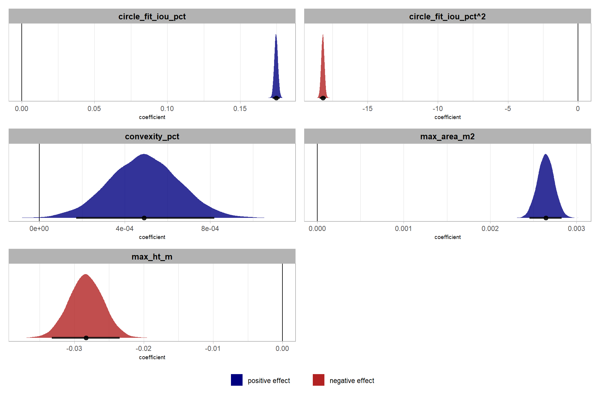
question 1: does CHM resolution influences detection accuracy?
to properly understand this question with our model, we must consider the credible slope of the CHM resolution predictor as a function of the spectral_weight parameter (e.g. Kurz 2025; Kruschke (2015, Ch. 18))
brms::as_draws_df(brms_f_score_mod) %>%
  dplyr::select(tidyselect::starts_with("b_")) %>%
  dplyr::mutate(
    dplyr::across(
      .cols = tidyselect::contains(":spectral_weight")
      , ~ .x + b_chm_res_m
    )
  ) %>%
  dplyr::select(tidyselect::starts_with("b_chm_res_m")) %>%
  tidyr::pivot_longer(dplyr::everything()) %>%
  dplyr::mutate(
    name = stringr::str_remove(name, "\\bb_")
    , spectral_weight =
      dplyr::case_when(
        # get the last character which is the spectral weight
        stringr::str_detect(name, ":spectral_weight") ~ stringr::str_sub(name, -1, -1)
        , T ~ "0"
      ) %>%
      as.numeric() %>%
      factor() %>%
      forcats::fct_rev()
  ) %>%
  dplyr::group_by(spectral_weight) %>%
  dplyr::mutate(
    median_hdi_est = tidybayes::median_hdi(value)$y
    , median_hdi_lower = tidybayes::median_hdi(value)$ymin
    , median_hdi_upper = tidybayes::median_hdi(value)$ymax
  ) %>%
  dplyr::ungroup() %>%
  dplyr::mutate(
    col_grp = dplyr::case_when(
      # 0>median_hdi_lower & 0<median_hdi_upper ~ "no effect"
       median_hdi_est==0 ~ "no effect"
      , median_hdi_est>0 ~ "positive effect"
      , median_hdi_est<0 ~ "negative effect"
    )
  ) %>%
  ggplot2::ggplot(
    mapping = ggplot2::aes(x = value, y = spectral_weight, fill = col_grp)
    # mapping = ggplot2::aes(x = value, y = name)
  ) +
  ggplot2::geom_vline(xintercept = 0, color = "black") +
  # ggplot2::geom_linerange(mapping = ggplot2::aes(xmin=median_hdi_lower, xmax=median_hdi_upper), lwd = 2) +
  tidybayes::stat_halfeye(
    point_interval = median_hdi, .width = .95
    , alpha = 0.8
    # , color = "firebrick"
    # , point_size = 4, lwd = 7
  ) +
  ggplot2::scale_color_manual(values = c("negative effect"="firebrick","no effect"="gray44","positive effect"="navy")) +
  ggplot2::scale_fill_manual(values = c("negative effect"="firebrick","no effect"="gray44","positive effect"="navy")) +
  ggplot2::labs(
    x = "slope of CHM resolution (`chm_res_m`)", y = "spectral_weight"
    , color = "", fill = ""
  ) +
  ggplot2::theme_light() +
  ggplot2::theme(
    legend.position = "bottom"
    , axis.title.x = ggplot2::element_text(size = 7)
  ) +
  ggplot2::guides(
    fill = ggplot2::guide_legend(override.aes = list(shape = NA, linetype = 0, size = 5, alpha = 1))
    , shape = "none"
    , color = "none"
  )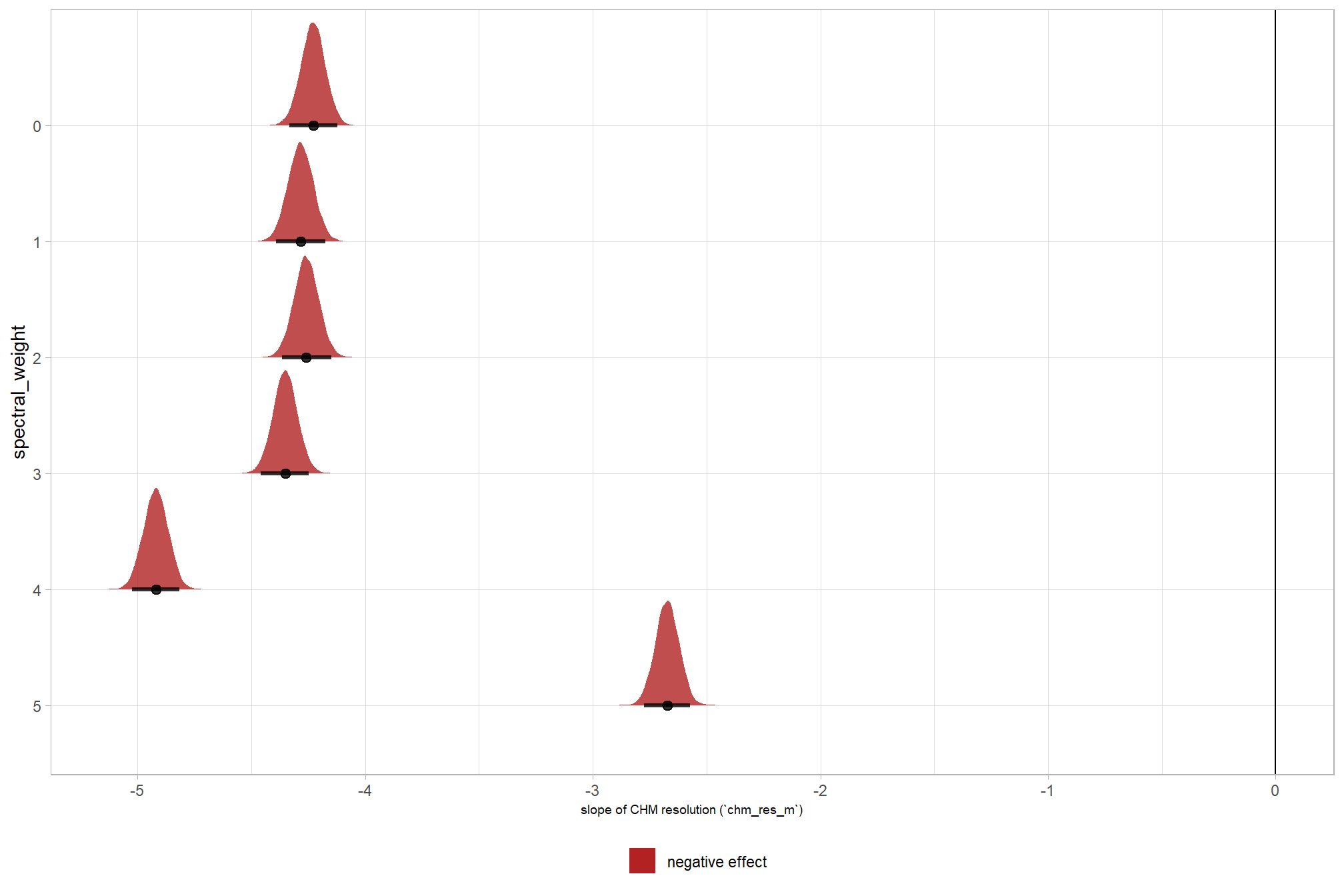
question 3: does the use of spectral data have a meaningful impact on detection and quantification accuracy
brms::as_draws_df(brms_f_score_mod) %>%
  dplyr::select(tidyselect::starts_with("b_spectral_weight")) %>%
  tidyr::pivot_longer(dplyr::everything()) %>%
  dplyr::mutate(
    name = stringr::str_remove(name, "\\bb_")
    , spectral_weight = stringr::str_sub(name, -1, -1) %>%
      as.numeric() %>%
      factor() %>%
      forcats::fct_rev()
  ) %>%
  dplyr::group_by(spectral_weight) %>%
  dplyr::mutate(
    median_hdi_est = tidybayes::median_hdi(value)$y
    , median_hdi_lower = tidybayes::median_hdi(value)$ymin
    , median_hdi_upper = tidybayes::median_hdi(value)$ymax
  ) %>%
  dplyr::ungroup() %>%
  dplyr::mutate(
    col_grp = dplyr::case_when(
      # 0>median_hdi_lower & 0<median_hdi_upper ~ "no effect"
      median_hdi_est==0 ~ "no"
      , median_hdi_est>0 ~ "positive"
      , median_hdi_est<0 ~ "negative"
    )
  ) %>%
  ggplot2::ggplot(
    mapping = ggplot2::aes(x = value, y = spectral_weight, fill = col_grp)
    # mapping = ggplot2::aes(x = value, y = name)
  ) +
  ggplot2::geom_vline(xintercept = 0, color = "black") +
  tidybayes::stat_halfeye(
    point_interval = median_hdi, .width = .95
    , alpha = 0.8
    # , color = "firebrick"
    # , point_size = 4, lwd = 7
  ) +
  ggplot2::scale_color_manual(values = c("negative"="firebrick","no"="gray44","positive"="navy")) +
  ggplot2::scale_fill_manual(values = c("negative"="firebrick","no"="gray44","positive"="navy")) +
  ggplot2::labs(
    x = "intercept", y = "spectral_weight"
    , color = "", fill = ""
  ) +
  ggplot2::theme_light() +
  ggplot2::theme(
    legend.position = "none"
    , axis.title.x = ggplot2::element_text(size = 7)
  ) +
  ggplot2::guides(
    fill = ggplot2::guide_legend(override.aes = list(shape = NA, linetype = 0, size = 5, alpha = 1))
    , shape = "none"
    , color = "none"
  )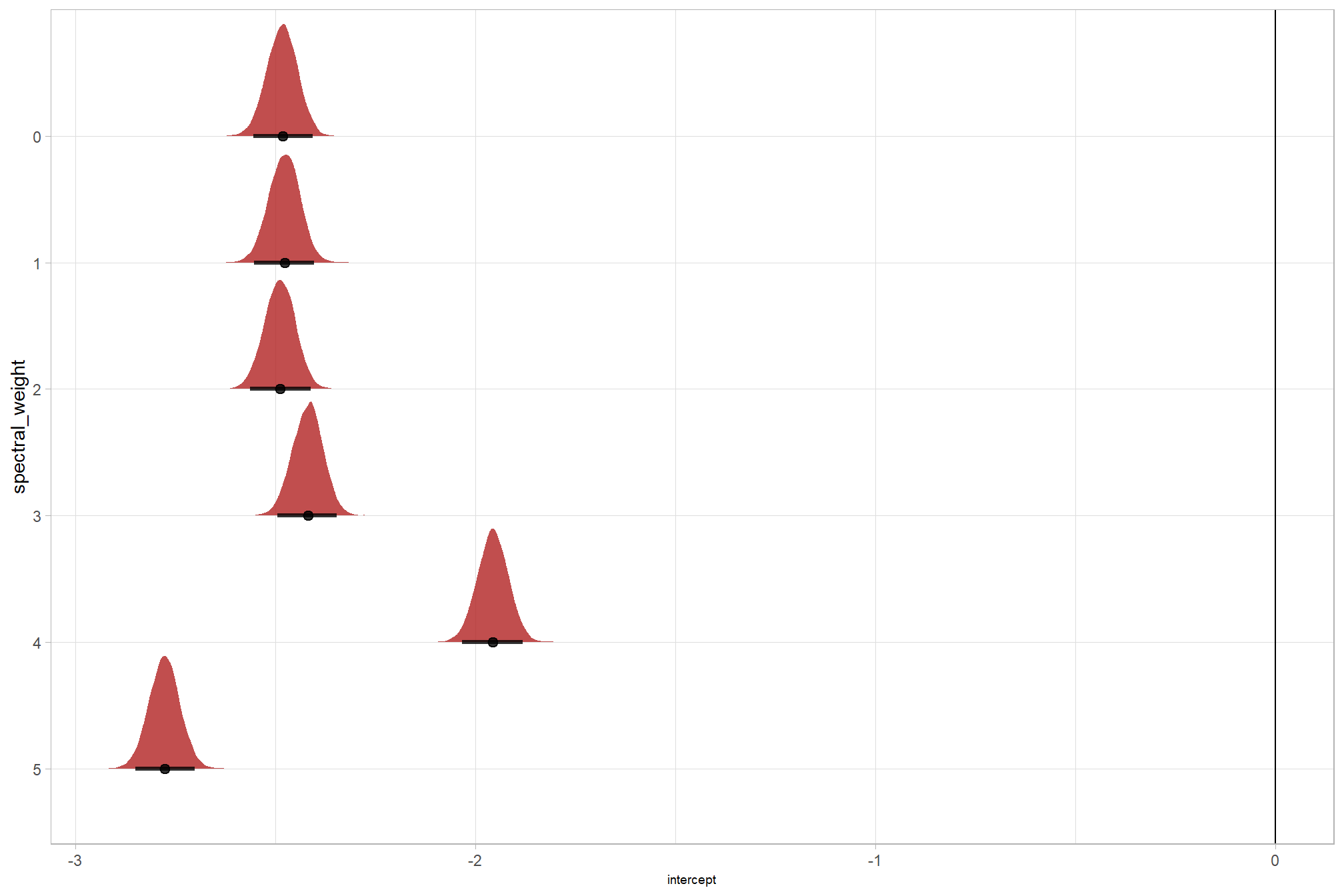
averaging across all other parameters to look at the main effect of including spectral data with the spectral_weight parameter, these results align with what we saw during our data summarization exploration: increasing the spectral_weight (where “5” requires all spectral index thresholds to be met) had minimal impact on metrics until a value of “3”, at which point F-score saw a minimal increase; at a spectral_weight of “4”, the F-score significantly improved, but at a value of “5” F-score was lower than not including the spectral data at all.
to actually compare the different levels of spectral_weight, we’ll use the MCMC draws to contrast the posterior predictions at different levels of the parameter (see below)
9.7.3 Posterior Predictive Expectation
we’re going to test our hypotheses with the posterior predictive distribution (i.e. posterior distributions of means)
to do this, we’ll fix the four structural parameters (e.g. max_ht_m and circle_fit_iou_pct) tested at the settings most frequently occurring in the top percentile of our detection+quantification accuracy assessment
# let's fix the structural parameters at the structural settings most frequently occurring
# in the top percentile of our detection+quantification accuracy assessment
structural_params_settings <-
  dplyr::bind_rows(
    # structural only
    param_combos_ranked %>% dplyr::filter(is_top_overall) %>% dplyr::select(max_ht_m,max_area_m2,convexity_pct,circle_fit_iou_pct)
    # fusion
    , param_combos_spectral_ranked %>%
      dplyr::ungroup() %>%
      dplyr::filter(is_top_overall & spectral_weight!=0) %>%
      dplyr::arrange(ovrall_balanced_rank) %>% # same number of records as structural only
      dplyr::filter(dplyr::row_number()<=sum(param_combos_ranked$is_top_overall)) %>%
      dplyr::select(max_ht_m,max_area_m2,convexity_pct,circle_fit_iou_pct)
  ) %>%
    tidyr::pivot_longer(
      cols = dplyr::everything()
      , names_to = "metric"
      , values_to = "value"
    ) %>%
    dplyr::count(metric, value) %>%
    dplyr::group_by(metric) %>%
    dplyr::arrange(metric,desc(n),value) %>%
    dplyr::slice(1) %>%
    dplyr::select(-n) %>%
    tidyr::pivot_wider(names_from = metric, values_from = value)
# huh?
structural_params_settings %>% dplyr::glimpse()
## Rows: 1
## Columns: 4
## $ circle_fit_iou_pct <dbl> 0.6
## $ convexity_pct <dbl> 0.7
## $ max_area_m2 <dbl> 10
## $ max_ht_m <dbl> 2get the posterior predictive draws
draws_temp <-
  tidyr::crossing(
    structural_params_settings
    , param_combos_spectral_gt_agg %>% dplyr::distinct(spectral_weight_fact, spectral_weight)
    , param_combos_spectral_gt_agg %>% dplyr::distinct(chm_res_m)
  ) %>%
  tidybayes::add_epred_draws(brms_f_score_mod) %>%
  dplyr::rename(value = .epred)
# # huh?
# draws_temp %>% dplyr::glimpse()
question 2: does the effect of CHM resolution change based on the inclusion of spectral data versus using only structural data?
first, we’ll look at the impact of changing CHM resolution by the spectral_weight parameter where a value of “0” indicates no spectral data was used (i.e. structural only), the lowest weighting of the spectral data is “1” (only one spectral index threshold must be met), and the highest weighting of spectral data is “5” (all spectral index thresholds must be met).
pal_spectral_weight <- c("gray77", harrypotter::hp(n=5, option = "gryffindor", direction = 1)) # %>%  scales::show_col()
# brms::posterior_summary(brms_f_score_mod)
draws_temp %>%
  ggplot2::ggplot(mapping = ggplot2::aes(x = chm_res_m, y = value, color = spectral_weight)) +
  # tidybayes::stat_halfeye() +
  tidybayes::stat_lineribbon(point_interval = "median_hdi", .width = c(0.95)) +
  # ggplot2::facet_wrap(facets = dplyr::vars(spectral_weight))
  ggplot2::scale_fill_brewer(palette = "Greys") +
  ggplot2::scale_color_manual(values = pal_spectral_weight) +
  ggplot2::scale_y_continuous(labels = scales::percent) +
  ggplot2::labs(x = "CHM resolution", y = "F-score") +
  ggplot2::theme_light() +
  ggplot2::theme(
    legend.position = "top"
  ) +
  ggplot2::guides(
    color = ggplot2::guide_legend(override.aes = list(shape = 15, lwd = 8, fill = NA))
    , fill = "none"
  )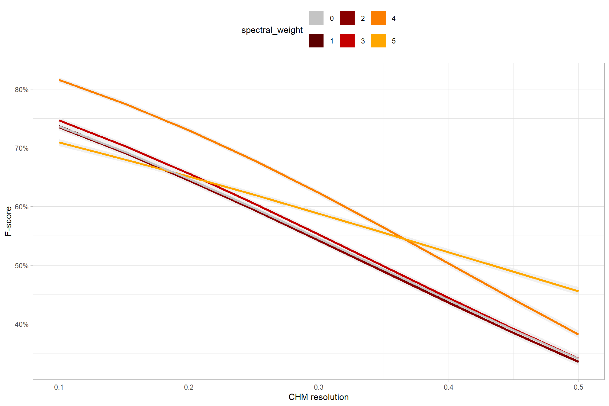
there are a few takeaways from this plot:
- including spectral data and setting the
spectral_weightto “1”, “2”, or “3” appears to be not much different than not including spectral data at all (but we’ll probabilistically test this) - including spectral data and setting the
spectral_weightto “4” yields a larger negative impact of decreasing CHM resolution on detection accuracy - including spectral data and setting the
spectral_weightto “5” yields a smaller negative impact of decreasing CHM resolution on detection accuracy and beyond a CHM resolution of ~0.375 m detection accuracy is maximized when setting thespectral_weightto “5”. this makes intuitive sense because as the structural information about slash piles becomes less fine grain (i.e. more coarse), we should put more weight into the spectral data for detecting slash piles
all of this is to say that the impact of CHM resolution varies based on the spectral_weight setting and vice-versa
let’s test including predictions at CHM resolutions outside of the bounds of the data tested (e.g. > 0.5 m resolution)
tidyr::crossing(
    structural_params_settings
    , param_combos_spectral_gt_agg %>% dplyr::distinct(spectral_weight_fact, spectral_weight)
    , chm_res_m = seq(0.1,1,by = 0.1)
  ) %>%
  tidybayes::add_epred_draws(brms_f_score_mod) %>%
  dplyr::rename(value = .epred) %>%
  ggplot2::ggplot(mapping = ggplot2::aes(x = chm_res_m, y = value, color = spectral_weight)) +
  # tidybayes::stat_halfeye() +
  tidybayes::stat_lineribbon(point_interval = "median_hdi", .width = c(0.95)) +
  # ggplot2::facet_wrap(facets = dplyr::vars(spectral_weight))
  ggplot2::scale_fill_brewer(palette = "Greys") +
  ggplot2::scale_color_manual(values = pal_spectral_weight) +
  ggplot2::scale_y_continuous(labels = scales::percent) +
  ggplot2::labs(x = "CHM resolution", y = "F-score") +
  ggplot2::theme_light() +
  ggplot2::theme(
    legend.position = "top"
  ) +
  ggplot2::guides(
    color = ggplot2::guide_legend(override.aes = list(shape = 15, lwd = 8, fill = NA))
    , fill = "none"
  )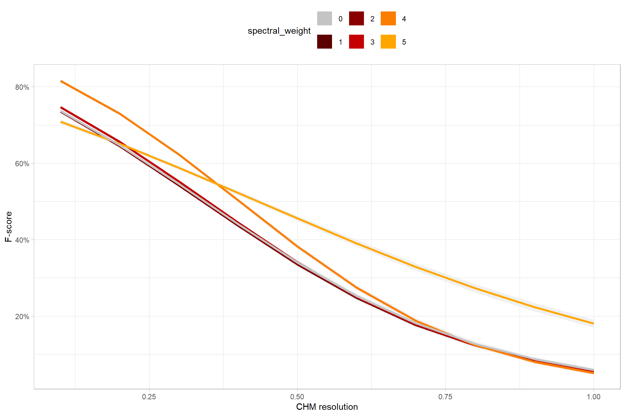
even at the coarse CHM resolutions not represented in the data, the model is still confident that increased resolution decreases detection accuracy
let’s make contrasts of the posterior predictions to probabilistically quantify the influence of CHM resolution at a given spectral weight. before we do this we’re going to borrow code from (Tinkham and Woolsey 2024) to make and plot the Bayesian contrasts
############################################
# make the variables for the contrast
############################################
make_contrast_vars = function(my_data){
  my_data %>%
    dplyr::mutate(
      # get median_hdi
      median_hdi_est = tidybayes::median_hdci(value)$y
      , median_hdi_lower = tidybayes::median_hdci(value)$ymin
      , median_hdi_upper = tidybayes::median_hdci(value)$ymax
      # check probability of contrast
      , pr_gt_zero = mean(value > 0) %>%
          scales::percent(accuracy = 1)
      , pr_lt_zero = mean(value < 0) %>%
          scales::percent(accuracy = 1)
      # check probability that this direction is true
      , is_diff_dir = dplyr::case_when(
        median_hdi_est >= 0 ~ value > 0
        , median_hdi_est < 0 ~ value < 0
      )
      , pr_diff = mean(is_diff_dir)
      # make a label
      , pr_diff_lab = dplyr::case_when(
          median_hdi_est > 0 ~ paste0(
            "Pr("
            , stringr::word(contrast, 1, sep = fixed("-")) %>%
              stringr::str_squish()
            , ">"
            , stringr::word(contrast, 2, sep = fixed("-")) %>%
              stringr::str_squish()
            , ")="
            , pr_diff %>% scales::percent(accuracy = 1)
          )
          , median_hdi_est < 0 ~ paste0(
            "Pr("
            , stringr::word(contrast, 2, sep = fixed("-")) %>%
              stringr::str_squish()
            , ">"
            , stringr::word(contrast, 1, sep = fixed("-")) %>%
              stringr::str_squish()
            , ")="
            , pr_diff %>% scales::percent(accuracy = 1)
          )
        )
      # make a SMALLER label
      , pr_diff_lab_sm = dplyr::case_when(
        median_hdi_est >= 0 ~ paste0(
          "Pr(>0)="
          , pr_diff %>% scales::percent(accuracy = 1)
        )
        , median_hdi_est < 0 ~ paste0(
          "Pr(<0)="
          , pr_diff %>% scales::percent(accuracy = 1)
        )
      )
      , pr_diff_lab_pos = dplyr::case_when(
        median_hdi_est > 0 ~ median_hdi_upper
        , median_hdi_est < 0 ~ median_hdi_lower
      ) * 1.075
      , sig_level = dplyr::case_when(
        pr_diff > 0.99 ~ 0
        , pr_diff > 0.95 ~ 1
        , pr_diff > 0.9 ~ 2
        , pr_diff > 0.8 ~ 3
        , T ~ 4
      ) %>%
      factor(levels = c(0:4), labels = c(">99%","95%","90%","80%","<80%"), ordered = T)
    )
}

############################################
# plot the contrast
############################################
plt_contrast <- function(
    my_data
    , x = "value"
    , y = "contrast"
    , fill = "pr_diff"
    , label = "pr_diff_lab"
    , label_pos = "pr_diff_lab_pos"
    , label_size = 3
    , x_expand = c(0.1, 0.1)
    , facet = NA
    , y_axis_title = ""
    , caption_text = "" # form_temp
    , annotate_size = 2.2
    , annotate_which = "both" # "both", "left", "right"
    ) {
  # df for annotation
  get_annotation_df <- function(
        my_text_list = c(
          "Bottom Left (h0,v0)","Top Left (h0,v1)"
          ,"Bottom Right h1,v0","Top Right h1,v1"
          )
        , hjust = c(0,0,1,1) # higher values = right, lower values = left
        , vjust = c(0,1.3,0,1.3) # higher values = down, lower values = up
    ){
      df = data.frame(
        xpos = c(-Inf,-Inf,Inf,Inf)
        , ypos =  c(-Inf, Inf,-Inf,Inf)
        , annotate_text = my_text_list
        , hjustvar = hjust
        , vjustvar = vjust
      )
      return(df)
  }

  if(annotate_which=="left"){
    text_list <- c(
      "","L.H.S. < R.H.S."
      ,"",""
    )
  }else if(annotate_which=="right"){
    text_list <- c(
      "",""
      ,"","L.H.S. > R.H.S."
    )
  }else{
    text_list <- c(
      "","L.H.S. < R.H.S."
      ,"","L.H.S. > R.H.S."
    )
  }

  # plot
  plt =
    my_data %>%
    ggplot(aes(x = .data[[x]], y = .data[[y]])) +
      geom_vline(xintercept = 0, linetype = "solid", color = "gray33", lwd = 1.1) +
      tidybayes::stat_halfeye(
        mapping = aes(fill = .data[[fill]])
        , point_interval = median_hdi, .width = c(0.5,0.95)
        # , slab_fill = "gray22", slab_alpha = 1
        , interval_color = "black", point_color = "black", point_fill = "black"
        , point_size = 0.9
        , justification = -0.01
      ) +
      geom_text(
        data = get_annotation_df(
          my_text_list = text_list
        )
        , mapping = aes(
          x = xpos, y = ypos
          , hjust = hjustvar, vjust = vjustvar
          , label = annotate_text
          , fontface = "bold"
        )
        , size = annotate_size
        , color = "gray30" # "#2d2a4d" #"#204445"
      ) +
      # scale_fill_fermenter(
      #   n.breaks = 5 # 10 use 10 if can go full range 0-1
      #   , palette = "PuOr" # "RdYlBu"
      #   , direction = 1
      #   , limits = c(0.5,1) # use c(0,1) if can go full range 0-1
      #   , labels = scales::percent
      # ) +
      scale_fill_stepsn(
        n.breaks = 5 # 10 use 10 if can go full range 0-1
        , colors = harrypotter::hp(n=5, option="ravenclaw", direction = -1) # RColorBrewer::brewer.pal(11,"PuOr")[c(3,4,8,10,11)]
        , limits = c(0.5,1) # use c(0,1) if can go full range 0-1
        , labels = scales::percent
      ) +
      scale_x_continuous(expand = expansion(mult = x_expand)) +
      labs(
        y = y_axis_title
        , x = "difference (F-score)"
        , fill = "Pr(contrast)"
        , subtitle = "posterior predictive distribution of group constrasts with 95% & 50% HDI"
        , caption = caption_text
      ) +
      theme_light() +
      theme(
        legend.text = element_text(size = 7)
        , legend.title = element_text(size = 8)
        , axis.text.x = element_text(angle = 90, vjust = 0.5, hjust = 1.05)
        , strip.text = element_text(color = "black", face = "bold")
      ) +
      guides(fill = guide_colorbar(theme = theme(
        legend.key.width  = unit(1, "lines"),
        legend.key.height = unit(12, "lines")
      )))

  # label or not
  if(!is.na(label) && !is.na(label_pos) && !is.na(label_size)){
    plt <- plt +
      geom_text(
          data = my_data %>%
            dplyr::filter(pr_diff_lab_pos>=0) %>%
            dplyr::ungroup() %>%
            dplyr::select(tidyselect::all_of(c(
              y
              , fill
              , label
              , label_pos
              , facet
            ))) %>%
            dplyr::distinct()
          , mapping = aes(x = .data[[label_pos]], label = .data[[label]])
          , vjust = -1, hjust = 0, size = label_size
        ) +
        geom_text(
          data = my_data %>%
            dplyr::filter(pr_diff_lab_pos<0) %>%
            dplyr::ungroup() %>%
            dplyr::select(tidyselect::all_of(c(
              y
              , fill
              , label
              , label_pos
              , facet
            ))) %>%
            dplyr::distinct()
          , mapping = aes(x = .data[[label_pos]], label = .data[[label]])
          , vjust = -1, hjust = +1, size = label_size
        )
  }

  # return facet or not
  if(max(is.na(facet))==0){
    return(
      plt +
        facet_grid(cols = vars(.data[[facet]]))
    )
  }
  else{return(plt)}
}
first, what is the impact of CHM resolution on detection accuracy based on the inclusion of spectral data?
contrast_temp <-
  draws_temp %>%
  dplyr::filter(
    round(chm_res_m,2) == round(chm_res_m,1) # let's just look at every 0.1 m (10 cm)
  ) %>%
  dplyr::group_by(spectral_weight) %>%
  tidybayes::compare_levels(
    value
    , by = chm_res_m
    , comparison =
      # tidybayes::emmeans_comparison("revpairwise")
      "pairwise"
  ) %>%
  # dplyr::glimpse()
  dplyr::rename(contrast = chm_res_m) %>%
  # group the data before calculating contrast variables %>%
  dplyr::group_by(spectral_weight, contrast) %>%
  make_contrast_vars() %>%
  # relabel the label for the facets
  dplyr::mutate(spectral_weight = forcats::fct_relabel(spectral_weight,~paste0("spectral_weight: ", .x, recycle0 = T)))
# huh?
# contrast_temp %>% dplyr::glimpse()

# plot it
plt_contrast(
  contrast_temp
  # , caption_text = form_temp
  , y_axis_title = "CHM resolution contrast"
  , facet = "spectral_weight"
  , label_size = NA
  , x_expand = c(0,0.1)
  , annotate_which = "left"
) +
  labs(
    subtitle = "posterior predictive distribution of group constrasts with 95% & 50% HDI\nby `spectral_weight`"
  )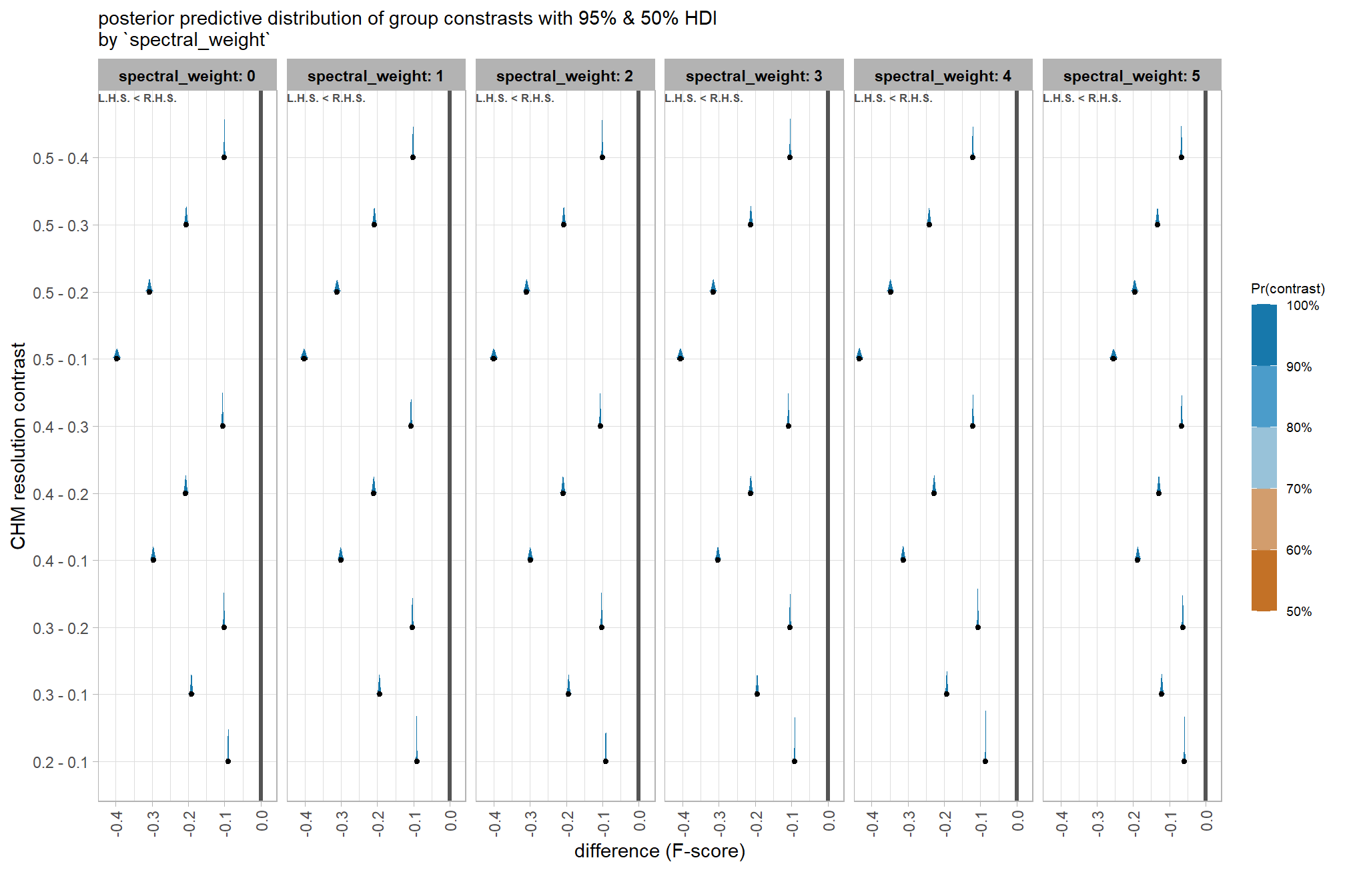
let’s table it
contrast_temp %>%
    dplyr::distinct(
      spectral_weight, contrast
      , median_hdi_est, median_hdi_lower, median_hdi_upper
      , pr_lt_zero # , pr_gt_zero
    ) %>%
    dplyr::arrange(spectral_weight, contrast) %>%
    kableExtra::kbl(
      digits = 2
      , caption = "brms::brm model: 95% HDI of the posterior predictive distribution of group constrasts"
      , col.names = c(
        "spectral_weight", "CHM res. contrast"
        , "difference (F-score)"
        , "HDI low", "HDI high"
        , "Pr(diff<0)"
      )
      , escape = F
    ) %>%
    kableExtra::kable_styling() %>%
    kableExtra::collapse_rows(columns = 1, valign = "top") %>%
kableExtra::scroll_box(height = "8in")| spectral_weight | CHM res. contrast | difference (F-score) | HDI low | HDI high | Pr(diff<0) |
|---|---|---|---|---|---|
| spectral_weight: 0 | 0.2 - 0.1 | -0.09 | -0.09 | -0.09 | 100% |
| 0.3 - 0.1 | -0.19 | -0.20 | -0.19 | 100% | |
| 0.3 - 0.2 | -0.10 | -0.10 | -0.10 | 100% | |
| 0.4 - 0.1 | -0.30 | -0.30 | -0.29 | 100% | |
| 0.4 - 0.2 | -0.21 | -0.21 | -0.20 | 100% | |
| 0.4 - 0.3 | -0.11 | -0.11 | -0.10 | 100% | |
| 0.5 - 0.1 | -0.40 | -0.40 | -0.39 | 100% | |
| 0.5 - 0.2 | -0.31 | -0.31 | -0.30 | 100% | |
| 0.5 - 0.3 | -0.21 | -0.21 | -0.20 | 100% | |
| 0.5 - 0.4 | -0.10 | -0.10 | -0.10 | 100% | |
| spectral_weight: 1 | 0.2 - 0.1 | -0.09 | -0.09 | -0.09 | 100% |
| 0.3 - 0.1 | -0.19 | -0.20 | -0.19 | 100% | |
| 0.3 - 0.2 | -0.10 | -0.11 | -0.10 | 100% | |
| 0.4 - 0.1 | -0.30 | -0.31 | -0.29 | 100% | |
| 0.4 - 0.2 | -0.21 | -0.21 | -0.20 | 100% | |
| 0.4 - 0.3 | -0.11 | -0.11 | -0.10 | 100% | |
| 0.5 - 0.1 | -0.40 | -0.41 | -0.39 | 100% | |
| 0.5 - 0.2 | -0.31 | -0.32 | -0.30 | 100% | |
| 0.5 - 0.3 | -0.21 | -0.21 | -0.20 | 100% | |
| 0.5 - 0.4 | -0.10 | -0.10 | -0.10 | 100% | |
| spectral_weight: 2 | 0.2 - 0.1 | -0.09 | -0.09 | -0.09 | 100% |
| 0.3 - 0.1 | -0.19 | -0.20 | -0.19 | 100% | |
| 0.3 - 0.2 | -0.10 | -0.10 | -0.10 | 100% | |
| 0.4 - 0.1 | -0.30 | -0.31 | -0.29 | 100% | |
| 0.4 - 0.2 | -0.21 | -0.21 | -0.20 | 100% | |
| 0.4 - 0.3 | -0.11 | -0.11 | -0.10 | 100% | |
| 0.5 - 0.1 | -0.40 | -0.41 | -0.39 | 100% | |
| 0.5 - 0.2 | -0.31 | -0.32 | -0.30 | 100% | |
| 0.5 - 0.3 | -0.21 | -0.21 | -0.20 | 100% | |
| 0.5 - 0.4 | -0.10 | -0.10 | -0.10 | 100% | |
| spectral_weight: 3 | 0.2 - 0.1 | -0.09 | -0.09 | -0.09 | 100% |
| 0.3 - 0.1 | -0.19 | -0.20 | -0.19 | 100% | |
| 0.3 - 0.2 | -0.10 | -0.11 | -0.10 | 100% | |
| 0.4 - 0.1 | -0.30 | -0.31 | -0.30 | 100% | |
| 0.4 - 0.2 | -0.21 | -0.22 | -0.21 | 100% | |
| 0.4 - 0.3 | -0.11 | -0.11 | -0.11 | 100% | |
| 0.5 - 0.1 | -0.41 | -0.41 | -0.40 | 100% | |
| 0.5 - 0.2 | -0.32 | -0.32 | -0.31 | 100% | |
| 0.5 - 0.3 | -0.21 | -0.22 | -0.21 | 100% | |
| 0.5 - 0.4 | -0.10 | -0.11 | -0.10 | 100% | |
| spectral_weight: 4 | 0.2 - 0.1 | -0.09 | -0.09 | -0.08 | 100% |
| 0.3 - 0.1 | -0.19 | -0.20 | -0.19 | 100% | |
| 0.3 - 0.2 | -0.11 | -0.11 | -0.10 | 100% | |
| 0.4 - 0.1 | -0.31 | -0.32 | -0.31 | 100% | |
| 0.4 - 0.2 | -0.23 | -0.23 | -0.22 | 100% | |
| 0.4 - 0.3 | -0.12 | -0.12 | -0.12 | 100% | |
| 0.5 - 0.1 | -0.43 | -0.44 | -0.43 | 100% | |
| 0.5 - 0.2 | -0.35 | -0.36 | -0.34 | 100% | |
| 0.5 - 0.3 | -0.24 | -0.25 | -0.24 | 100% | |
| 0.5 - 0.4 | -0.12 | -0.12 | -0.12 | 100% | |
| spectral_weight: 5 | 0.2 - 0.1 | -0.06 | -0.06 | -0.06 | 100% |
| 0.3 - 0.1 | -0.12 | -0.13 | -0.12 | 100% | |
| 0.3 - 0.2 | -0.06 | -0.07 | -0.06 | 100% | |
| 0.4 - 0.1 | -0.19 | -0.19 | -0.18 | 100% | |
| 0.4 - 0.2 | -0.13 | -0.13 | -0.12 | 100% | |
| 0.4 - 0.3 | -0.07 | -0.07 | -0.06 | 100% | |
| 0.5 - 0.1 | -0.25 | -0.26 | -0.24 | 100% | |
| 0.5 - 0.2 | -0.20 | -0.20 | -0.19 | 100% | |
| 0.5 - 0.3 | -0.13 | -0.14 | -0.13 | 100% | |
| 0.5 - 0.4 | -0.07 | -0.07 | -0.06 | 100% |
now, what is the impact of the inclusion of spectral data on detection accuracy based on the CHM resolution?
contrast_temp <-
  draws_temp %>%
  dplyr::filter(
    round(chm_res_m,2) == round(chm_res_m,1) # let's just look at every 0.1 m (10 cm)
  ) %>%
  dplyr::group_by(chm_res_m) %>%
  tidybayes::compare_levels(
    value
    , by = spectral_weight
    , comparison =
      # tidybayes::emmeans_comparison("revpairwise")
      "pairwise"
  ) %>%
  # dplyr::glimpse()
  dplyr::rename(contrast = spectral_weight) %>%
  # group the data before calculating contrast variables %>%
  dplyr::group_by(chm_res_m, contrast) %>%
  make_contrast_vars() %>%
  # relabel the label for the facets
  dplyr::mutate(chm_res_m = chm_res_m %>% factor() %>% forcats::fct_relabel(~paste0("CHM resolution: ", .x, recycle0 = T)))
# huh?
# contrast_temp %>% dplyr::glimpse()

# plot it
plt_contrast(
  contrast_temp
  # , caption_text = form_temp
  , y_axis_title = "`spectral_weight` contrast"
  , facet = "chm_res_m"
  , label_size = 2
  , x_expand = c(0.5,0.5)
) +
  labs(
    subtitle = "posterior predictive distribution of group constrasts with 95% & 50% HDI\nby `chm_res_m`"
  )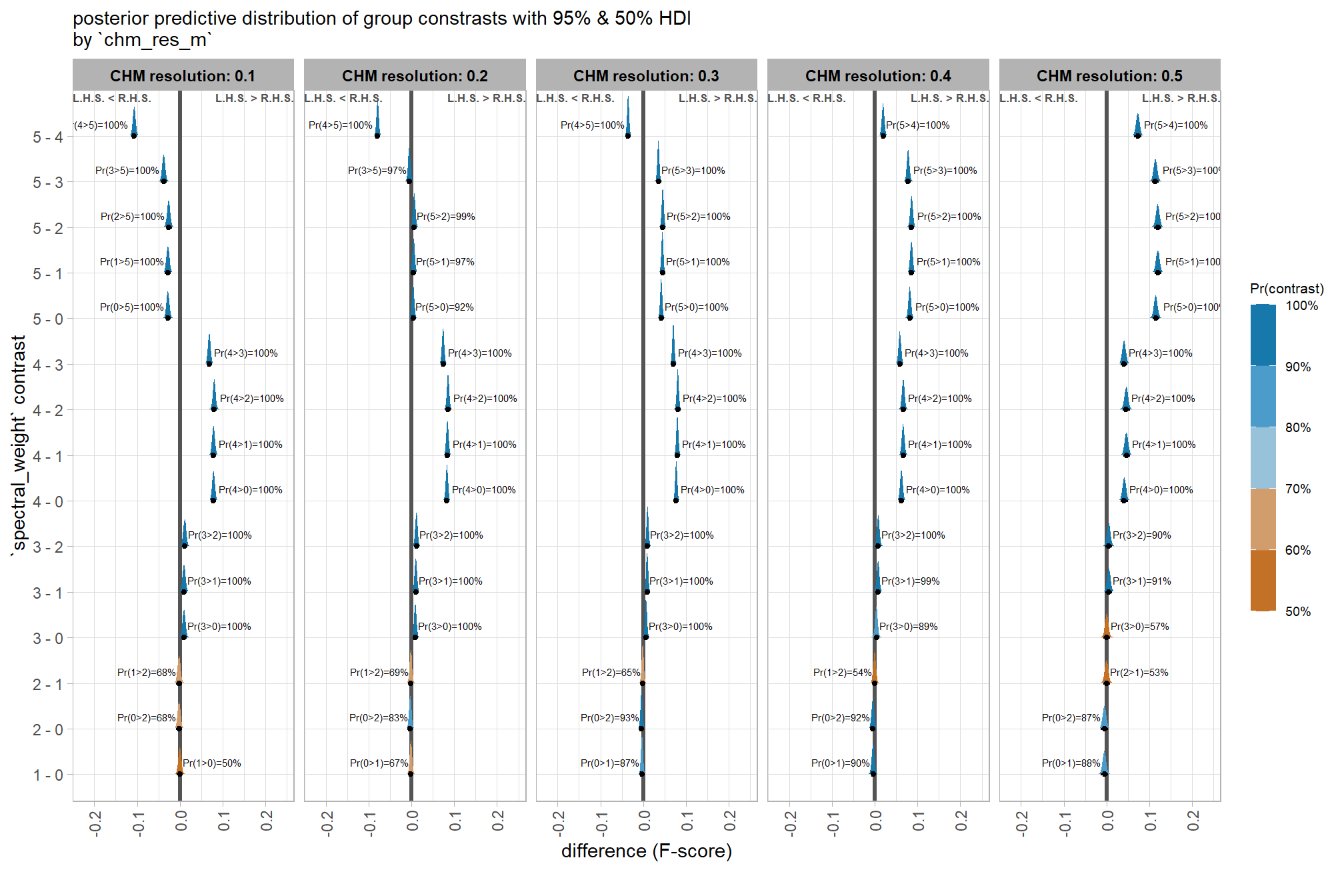
let’s table it
contrast_temp %>%
    dplyr::distinct(
      chm_res_m, contrast
      , median_hdi_est, median_hdi_lower, median_hdi_upper
      # , pr_lt_zero
      , pr_gt_zero
    ) %>%
    dplyr::arrange(chm_res_m, contrast) %>%
    kableExtra::kbl(
      digits = 2
      , caption = "brms::brm model: 95% HDI of the posterior predictive distribution of group constrasts"
      , col.names = c(
        "CHM resolution", "spectral_weight"
        , "difference (F-score)"
        , "HDI low", "HDI high"
        # , "Pr(diff<0)"
        , "Pr(diff>0)"
      )
      , escape = F
    ) %>%
    kableExtra::kable_styling() %>%
    kableExtra::collapse_rows(columns = 1, valign = "top") %>%
kableExtra::scroll_box(height = "8in")| CHM resolution | spectral_weight | difference (F-score) | HDI low | HDI high | Pr(diff>0) |
|---|---|---|---|---|---|
| CHM resolution: 0.1 | 1 - 0 | 0.00 | -0.01 | 0.01 | 50% |
| 2 - 0 | 0.00 | -0.01 | 0.01 | 32% | |
| 2 - 1 | 0.00 | -0.01 | 0.01 | 32% | |
| 3 - 0 | 0.01 | 0.00 | 0.02 | 100% | |
| 3 - 1 | 0.01 | 0.00 | 0.02 | 100% | |
| 3 - 2 | 0.01 | 0.00 | 0.02 | 100% | |
| 4 - 0 | 0.08 | 0.07 | 0.09 | 100% | |
| 4 - 1 | 0.08 | 0.07 | 0.09 | 100% | |
| 4 - 2 | 0.08 | 0.07 | 0.09 | 100% | |
| 4 - 3 | 0.07 | 0.06 | 0.07 | 100% | |
| 5 - 0 | -0.03 | -0.03 | -0.02 | 0% | |
| 5 - 1 | -0.03 | -0.03 | -0.02 | 0% | |
| 5 - 2 | -0.03 | -0.03 | -0.02 | 0% | |
| 5 - 3 | -0.04 | -0.04 | -0.03 | 0% | |
| 5 - 4 | -0.11 | -0.11 | -0.10 | 0% | |
| CHM resolution: 0.2 | 1 - 0 | 0.00 | -0.01 | 0.00 | 33% |
| 2 - 0 | 0.00 | -0.01 | 0.00 | 17% | |
| 2 - 1 | 0.00 | -0.01 | 0.00 | 31% | |
| 3 - 0 | 0.01 | 0.00 | 0.01 | 100% | |
| 3 - 1 | 0.01 | 0.00 | 0.02 | 100% | |
| 3 - 2 | 0.01 | 0.01 | 0.02 | 100% | |
| 4 - 0 | 0.08 | 0.08 | 0.09 | 100% | |
| 4 - 1 | 0.08 | 0.08 | 0.09 | 100% | |
| 4 - 2 | 0.09 | 0.08 | 0.09 | 100% | |
| 4 - 3 | 0.07 | 0.07 | 0.08 | 100% | |
| 5 - 0 | 0.00 | 0.00 | 0.01 | 92% | |
| 5 - 1 | 0.01 | 0.00 | 0.01 | 97% | |
| 5 - 2 | 0.01 | 0.00 | 0.01 | 99% | |
| 5 - 3 | -0.01 | -0.01 | 0.00 | 3% | |
| 5 - 4 | -0.08 | -0.08 | -0.07 | 0% | |
| CHM resolution: 0.3 | 1 - 0 | 0.00 | -0.01 | 0.00 | 13% |
| 2 - 0 | 0.00 | -0.01 | 0.00 | 7% | |
| 2 - 1 | 0.00 | -0.01 | 0.00 | 35% | |
| 3 - 0 | 0.01 | 0.00 | 0.01 | 100% | |
| 3 - 1 | 0.01 | 0.00 | 0.01 | 100% | |
| 3 - 2 | 0.01 | 0.01 | 0.02 | 100% | |
| 4 - 0 | 0.08 | 0.07 | 0.08 | 100% | |
| 4 - 1 | 0.08 | 0.08 | 0.08 | 100% | |
| 4 - 2 | 0.08 | 0.08 | 0.09 | 100% | |
| 4 - 3 | 0.07 | 0.07 | 0.08 | 100% | |
| 5 - 0 | 0.04 | 0.04 | 0.05 | 100% | |
| 5 - 1 | 0.04 | 0.04 | 0.05 | 100% | |
| 5 - 2 | 0.05 | 0.04 | 0.05 | 100% | |
| 5 - 3 | 0.04 | 0.03 | 0.04 | 100% | |
| 5 - 4 | -0.04 | -0.04 | -0.03 | 0% | |
| CHM resolution: 0.4 | 1 - 0 | 0.00 | -0.01 | 0.00 | 10% |
| 2 - 0 | 0.00 | -0.01 | 0.00 | 8% | |
| 2 - 1 | 0.00 | -0.01 | 0.01 | 46% | |
| 3 - 0 | 0.00 | 0.00 | 0.01 | 89% | |
| 3 - 1 | 0.01 | 0.00 | 0.01 | 99% | |
| 3 - 2 | 0.01 | 0.00 | 0.01 | 100% | |
| 4 - 0 | 0.06 | 0.06 | 0.07 | 100% | |
| 4 - 1 | 0.07 | 0.06 | 0.07 | 100% | |
| 4 - 2 | 0.07 | 0.06 | 0.07 | 100% | |
| 4 - 3 | 0.06 | 0.05 | 0.06 | 100% | |
| 5 - 0 | 0.08 | 0.08 | 0.09 | 100% | |
| 5 - 1 | 0.09 | 0.08 | 0.09 | 100% | |
| 5 - 2 | 0.09 | 0.08 | 0.09 | 100% | |
| 5 - 3 | 0.08 | 0.07 | 0.08 | 100% | |
| 5 - 4 | 0.02 | 0.01 | 0.03 | 100% | |
| CHM resolution: 0.5 | 1 - 0 | 0.00 | -0.01 | 0.00 | 12% |
| 2 - 0 | 0.00 | -0.01 | 0.00 | 13% | |
| 2 - 1 | 0.00 | -0.01 | 0.01 | 53% | |
| 3 - 0 | 0.00 | -0.01 | 0.01 | 57% | |
| 3 - 1 | 0.01 | 0.00 | 0.01 | 91% | |
| 3 - 2 | 0.01 | 0.00 | 0.01 | 90% | |
| 4 - 0 | 0.04 | 0.03 | 0.05 | 100% | |
| 4 - 1 | 0.05 | 0.04 | 0.05 | 100% | |
| 4 - 2 | 0.05 | 0.04 | 0.05 | 100% | |
| 4 - 3 | 0.04 | 0.03 | 0.05 | 100% | |
| 5 - 0 | 0.12 | 0.11 | 0.12 | 100% | |
| 5 - 1 | 0.12 | 0.11 | 0.13 | 100% | |
| 5 - 2 | 0.12 | 0.11 | 0.13 | 100% | |
| 5 - 3 | 0.11 | 0.11 | 0.12 | 100% | |
| 5 - 4 | 0.07 | 0.06 | 0.08 | 100% |
let’s identify the optimal spectral weight to use at a certain CHM resolution and then highlight the contrast between this optimal spectral_weight setting and not including any spectral data at all (i.e. structural data only)
draws_temp %>%
  dplyr::mutate(chm_res_m = chm_res_m %>% factor() %>% forcats::fct_relabel(~paste0("CHM resolution: ", .x, recycle0 = T))) %>%
  ggplot2::ggplot(mapping = ggplot2::aes(y=value, x=spectral_weight)) +
  tidybayes::stat_eye(
    mapping = ggplot2::aes(fill = spectral_weight)
    , point_interval = median_hdi, .width = .95
    , slab_alpha = 0.95
    , interval_color = "gray44", linewidth = 1
    , point_color = "gray44", point_fill = "gray44", point_size = 1
  ) +
  ggplot2::facet_grid(cols = dplyr::vars(chm_res_m)) +
  ggplot2::scale_fill_manual(values = pal_spectral_weight) +
  ggplot2::scale_y_continuous(labels = scales::percent) +
  ggplot2::labs(x = "spectral_weight", y = "F-score") +
  ggplot2::theme_light() +
  ggplot2::theme(
    legend.position = "none"
    , strip.text = ggplot2::element_text(size = 8, color = "black", face = "bold")
  )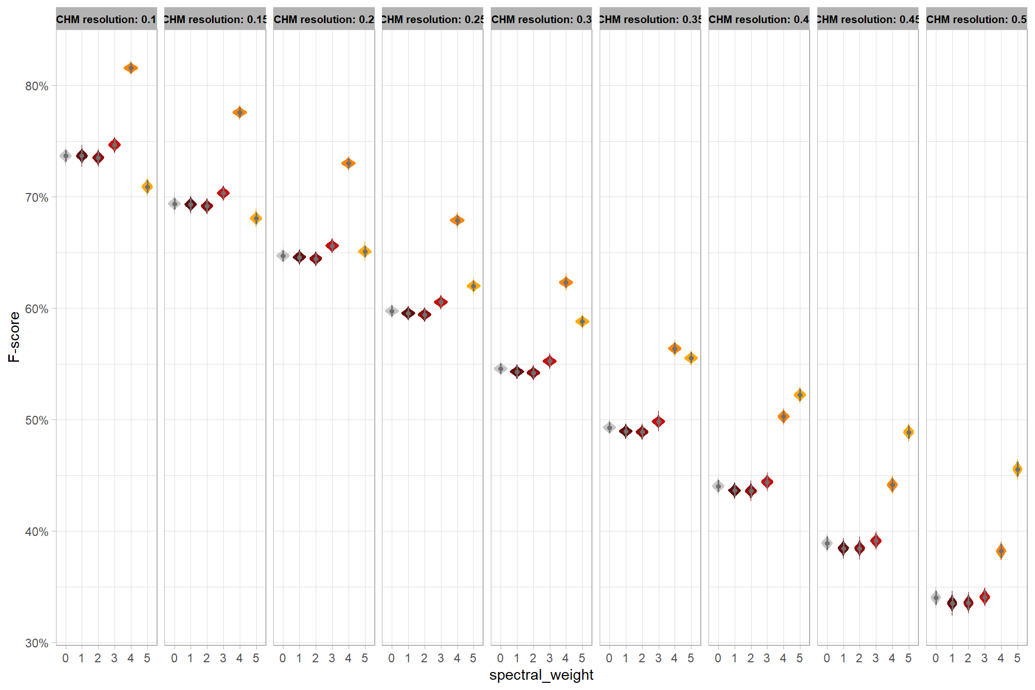
let’s table this and save the information
draws_temp %>%
  dplyr::group_by(chm_res_m,spectral_weight) %>%
  dplyr::summarise(
    # get median_hdi
    median_hdi_est = tidybayes::median_hdci(value)$y
    , median_hdi_lower = tidybayes::median_hdci(value)$ymin
    , median_hdi_upper = tidybayes::median_hdci(value)$ymax
  ) %>%
  dplyr::glimpse()
  dplyr::distinct(
    chm_res_m,spectral_weight,tidyselect
  )
#
# contrast_temp %>% dplyr::glimpse()
#     dplyr::distinct(
#       chm_res_m, contrast
#       , median_hdi_est, median_hdi_lower, median_hdi_upper
#       # , pr_lt_zero
#       , pr_gt_zero
#     ) %>%
#   dplyr::glimpse()