Section 6 Watershed Segmentation: Sensitivity Testing
Now we’ll perform sensitivity testing of our rules-based slash pile detection methodology which uses a CHM input raster generated directly from the aerial point cloud data. This method does not require any training data for model building and can potentially be used broadly across different domains.
The rule-based method for slash pile detection using CHM raster data generally follows this outline:
- CHM Generation: A Canopy Height Model (CHM) is generated from the point cloud data. The CHM is generated by removing the ground surface effectively representing a Digital Surface Model (DSM) without ground, ensuring all values are heights above bare earth.
- CHM Height Filtering: A maximum height filter is applied to the CHM to retaining only raster cells below a maximum expected slash pile height (e.g. 4 m), isolating a “slice” of the CHM.
- Candidate Segmentation: Watershed segmentation is performed on the filtered CHM raster to identify and delineate initial candidate piles based on their structural form.
- First Irregularity Filtering: Candidate pile locations are initially filtered to remove highly irregular shapes by assessing their overlap with their convex hull (e.g. >70% overlap). This step helps exclude lower tree branches (objects with holes in the lower CHM slice) and unorganized coarse woody debris.
- Area Filtering: A filter is applied based on the minimum and maximum expected pile areas.
- Circularity Filtering: A final geometric screen uses least squares circle fitting on each candidate pile, removing any that do not have a strong overlap (based on an Intersection over Union, or IoU, threshold) with the best-fit circle (e.g., >50%). This removes non-circular features such as rectangular boulders and downed tree stems.
* Raster Smoothing: The remaining segmented candidate raster is smoothed to generalize boundaries and aggregate disconnected segments. This process is only applied when the smoothing window (requiring a minimum window size of 3x3 raster cells) would be less than or equal to half the expected minimum pile area, ensuring that coarser rasters are not over-smoothed, which would increase the chance of including non-pile areas.* Second Irregularity and Area Filtering: A second pass of the area and irregularity filtering, using the convex hull process, is applied to remove any new irregular shapes that may have been generated during the smoothing - Shape Refinement & Overlap Removal: Lastly, segments are smoothed using their convex hull to remove the “blocky” raster edges (like they were made in Minecraft). Overlapping convex hull shapes are then removed to prevent false positives from clustered small trees or shrubs, ensuring singular pile detections.
the raster smoothing of the filtered segments worked well at very low chm resolutions (<=0.2m) for improving f-score and stabilizing slash pile footprint predictions when comparing the estimated diameter to field-measured values. however, at resolutions around 0.2 m, this process led to overestimation of pile diameter and a distorted trend in our accuracy metrics when compared across CHM resolutions. as a result, we have removed the raster smoothing step. our final detection process now relies on smoothing the filtered segments using their convex hull to remove “blocky” raster edges. the removal of any overlapping shapes is then used as the final step to prevent false positives from clustered small trees or shrubs.
6.1 Watershed Pile Detection Function
Let’s package all of the steps we demonstrated when formulating the methodology into a single function which can possibly be integrated into the cloud2trees package.
The parameters are defined as follows:
max_ht_m: numeric. The maximum height (in meters) a slash pile is expected to be. This value helps us focus on a specific “slice” of the data, ignoring anything taller than a typical pile.min_area_m2: numeric. The smallest 2D area (in square meters) a detected pile must cover to be considered valid.max_area_m2: numeric. The largest 2D area (in square meters) a detected pile can cover to be considered valid.convexity_pct: numeric. A value between 0 and 1 that controls how strict the filtering is for regularly shaped piles. A value of 1 means only piles that are perfectly smooth and rounded, with no dents or inward curves are kept. A value of 0 allows for both perfectly regular and very irregular shapes. This filter works alongsidecircle_fit_iou_pctto refine the pile’s overall shape.circle_fit_iou_pct: numeric. A value between 0 and 1 that controls how the filtering is for circular pile shapes. Setting it to 1 means only piles that are perfectly circular are kept. A value of 0 allows for a wide range of shapes, including very circular and non-circular ones (like long, straight lines).smooth_segs: logical. Setting this option to TRUE will: 1) smooth out the “blocky” edges of detected piles (which can look like they were made in Minecraft) by using their overall shape; and 2) remove any detected piles that overlap significantly with other smoothed piles to help ensure each detection is a single slash pile, not a cluster of small trees or shrubs.
# function to calculate the diamater of an sf polygon that is potentially irregularly shaped
# using the distance between the farthest points
st_calculate_diameter <- function(polygon) {
  # compute the convex hull
  ch <- sf::st_convex_hull(polygon)

  # cast to multipoint then point to get individual vertices
  ch_points <- sf::st_cast(sf::st_cast(ch, 'MULTIPOINT'), 'POINT')

  # calculate the distances between all pairs of points
  distances <- sf::st_distance(ch_points)

  # find the maximum distance, which is the diameter
  diameter <- as.numeric(max(distances,na.rm=T))
  return(diameter)
}
# rounds to nearest odd since ws for terra::focal() only takes odd
round_to_nearest_odd <- function(x) {
  rounded_int <- round(x)

  # step 2: check if the rounded integer is already odd
  is_odd <- (rounded_int %% 2 != 0)

  # step 3: for numbers that rounded to an even integer, find the nearest odd
  odd_down <- rounded_int - 1
  odd_up <- rounded_int + 1

  # calculate the absolute distances from the original number 'x'
  dist_down <- abs(x - odd_down)
  dist_up <- abs(x - odd_up)

  # step 4: use ifelse for vectorized conditional logic
  result <- ifelse(
    is_odd
    , rounded_int # if the initially rounded integer is odd, use it
    , ifelse(
      dist_down < dist_up
      , odd_down # if odd_down is strictly closer
      , odd_up # if odd_up is closer or equidistant
    )
  )

  return(result)
}
# round_to_nearest_odd(c(2,2.2,1.5,0))

# find window size given res and min expected area
ws_for_smooth_fn <- function(chm_res,min_area_m2){
  if(length(min_area_m2)>1){stop("min_area_m2 must be a single numeric value")}
  # return
  dplyr::case_when(
    T ~ 0 ## all will be 0 so smoothing won't happen
    ###!!!!!! original attempt down here...just remove T ~ 0 !!!!!!###
    , (chm_res*3) > (min_area_m2/2) ~ 0 # the minimum ws of 3 exceeds half of the expected area (coarse)
    , T ~ round( (min_area_m2/4) / chm_res ) %>% round_to_nearest_odd() %>% max(3) # has to be odd and at least 3
  )
}
# dplyr::tibble(res = seq(0.01,0.5,by=0.01)) %>%
#   dplyr::rowwise() %>%
#   dplyr::mutate(
#     ws = ws_for_smooth_fn(res, 2) # min_area_m2=2
#     , area = ifelse(ws==0, res*res,
#       (res^2) * (ws^2))
#     , area_prop = area/2 # min_area_m2=2
#   ) %>%
# ggplot() +
#   # geom_line(aes(x=res,y=ws)) +
#   # geom_line(aes(x=res,y=area)) +
#   geom_line(aes(x=res,y=area_prop)) +
#   # scale_y_continuous(breaks = scales::breaks_extended(n=22)) +
#   scale_y_continuous(breaks = scales::breaks_extended(n=22), labels = scales::percent) +
#   scale_x_continuous(breaks = scales::breaks_extended(n=20))


# detect funciton
slash_pile_detect_watershed <- function(
  chm_rast
  #### height and area thresholds for the detected piles
  # these should be based on data from the literature or expectations based on the prescription
  , max_ht_m = 4 # set the max expected pile height (could also do a minimum??)
  , min_area_m2 = 2 # set the min expected pile area
  , max_area_m2 = 50 # set the max expected pile area
  #### irregularity filtering
  # 1 = perfectly convex (no inward angles); 0 = so many inward angles
  # values closer to 1 remove more irregular segments;
    # values closer to 0 keep more irregular segments (and also regular segments)
  # these will all be further filtered for their circularity and later smoothed to remove blocky edges
  # and most inward angles by applying a convex hull to the original detected segment
  , convexity_pct = 0.7 # min required overlap between the predicted pile and the convex hull of the predicted pile
  #### circularity filtering
  # 1 = perfectly circular; 0 = not circular (e.g. linear) but also circular
  # min required IoU between the predicted pile and the best fit circle of the predicted pile
  , circle_fit_iou_pct = 0.5
  #### shape refinement & overlap removal
  ## smooth_segs = T ... convex hulls of raster detected segments are returned, any that overlap are removed
  ## smooth_segs = F ... raster detected segments are returned (blocky) if they meet all prior rules
  , smooth_segs = T
) {
    # checks
  if(!inherits(chm_rast,"SpatRaster")){stop("`chm_rast` must be raster data with the class `SpatRaster` ")}
  # just get the first layer and "slice" the raster based on the height threshold
  chm_rast <- chm_rast %>%
    terra::subset(subset = 1) %>%
    terra::clamp(upper = max_ht_m, lower = 0, values = F)

  # could make this a parameter
  # could automatically adjust for raster cell size:
    # higher res (smaller cell size) get bigger ws, lower res (larger cell size) get smaller/no ws???
  # get resolution which will be used to test against the minimum expected pile area
  chm_res <- max(terra::res(chm_rast)[1:2],na.rm = T)

  ws_for_smooth <- ws_for_smooth_fn(chm_res = chm_res, min_area_m2 = min_area_m2) # 3 # needs to be the same for the watershed seg and CHM smooth
  # search_area = (res^2) * (ws^2)

  ########################################################################################
  ## 1) watershed segmentation
  ########################################################################################
    # let's run watershed segmentation using `lidR::watershed()` which is based on the bioconductor package `EBIimage`
    # return is a raster with the first layer representing the identified watershed segments
    watershed_ans <- lidR::watershed(
        chm = chm_rast
        , th_tree = 0.5 # this would be the minimum expected pile height
      )()
    names(watershed_ans) <- "pred_id"

    # vectors of segments
    watershed_ans_poly <-
      watershed_ans %>%
      terra::as.polygons(round = F, aggregate = T, values = T, extent = F, na.rm = T) %>%
      setNames("pred_id") %>%
      sf::st_as_sf() %>%
      sf::st_simplify() %>%
      sf::st_make_valid() %>%
      dplyr::filter(sf::st_is_valid(.)) %>%
      # simplify multipolygons by keeping the largest polygon of each multipolygon
      dplyr::mutate(treeID=pred_id) %>%
      cloud2trees::simplify_multipolygon_crowns() %>%
      dplyr::select(-treeID)

  ########################################################################################
  ## 2) irregularity filtering
  ########################################################################################
    # let's first filter out segments that have holes in them
    # or are very irregularly shaped by comparing the area of the polygon and convex hull

    # convexity_pct = min required overlap between the predicted pile and the convex hull of the predicted pile
    if(convexity_pct>0){
      # apply the irregularity filtering on the polygons
      watershed_ans_poly <- watershed_ans_poly %>%
        st_irregular_remove(pct_chull_overlap = convexity_pct)
    }

    # check return
    if(dplyr::coalesce(nrow(watershed_ans_poly),0)==0){
      stop(paste0(
        "no segments detected using the given CHM and irregularity expectations"
        , "\n     try adjusting `convexity_pct` "
      ))
    }

  ########################################################################################
  ## 3) area filtering
  ########################################################################################
    # filter out the segments that don't meet the size thresholds
    watershed_ans_poly <- watershed_ans_poly %>%
      dplyr::mutate(area_xxxx = sf::st_area(.) %>% as.numeric()) %>%
      dplyr::filter(
        dplyr::coalesce(area_xxxx,0) >= min_area_m2
        & dplyr::coalesce(area_xxxx,0) <= max_area_m2
      ) %>%
      dplyr::select(-c(area_xxxx))

  ########################################################################################
  ## 4) circularity filtering
  ########################################################################################
    # let's apply a circle-fitting algorithm to remove non-circular segments from the remaining segments
    # let's apply the `sf_data_circle_fit()` function that
    # fits the best circle using `lidR::fit_circle()` to each watershed detected segment
    # to get a spatial data frame with the best fitting circle for each segment

    # apply the sf_data_circle_fit() which takes each segment polygon, transforms it to points, and the fits the best circle
    watershed_ans_poly_circle_fit <- sf_data_circle_fit(watershed_ans_poly)

    # filter using the intersection over union (IoU) between the circle and the predicted segment.
    # we'll use the IoU function we defined
    # we map over this to only compare the segment to it's own best circle fit...not all
    # we should consider doing this in bulk.....another day
    watershed_circle_fit_iou <-
      watershed_ans_poly$pred_id %>%
      unique() %>%
      purrr::map(\(x)
        ground_truth_single_match(
          gt_inst = watershed_ans_poly %>%
            dplyr::filter(pred_id == x)
          , gt_id = "pred_id"
          , predictions = watershed_ans_poly_circle_fit %>%
            dplyr::filter(pred_id == x) %>%
            dplyr::select(pred_id) %>% # keeping other columns causes error?
            dplyr::rename(circ_pred_id = pred_id)
          , pred_id = "circ_pred_id"
          , min_iou_pct = 0 # set to 0 just to return pct
        )
      ) %>%
      dplyr::bind_rows()

    # threshold for the minimum IoU to further filter for segments that are approximately round,
    # this filter should remove linear objects from the watershed detections
      # compare iou
      if(circle_fit_iou_pct==0){
        watershed_keep_circle_fit_pred_id <- watershed_keep_overlaps_chull_pred_id
      }else{
        watershed_keep_circle_fit_pred_id <- watershed_circle_fit_iou %>%
          dplyr::filter(iou>=circle_fit_iou_pct) %>%
          dplyr::pull(pred_id)
      }

    if(
      identical(watershed_keep_circle_fit_pred_id, numeric(0))
      || any(is.null(watershed_keep_circle_fit_pred_id))
      || any(is.na(watershed_keep_circle_fit_pred_id))
      || length(watershed_keep_circle_fit_pred_id)<1
    ){
      stop(paste0(
        "no segments detected using the given CHM and circularity expectations"
        , "\n     try adjusting `circle_fit_iou_pct` "
      ))
    }

  ########################################################################################
  ## 5) raster smoothing
  ########################################################################################
    ########################################
    # use the remaining segments that meet the geometric and area filtering
    # to smooth the watershed raster
    ########################################
    smooth_watershed_ans <- watershed_ans %>%
      terra::mask(
        watershed_ans_poly %>% #these are irregularity and area filtered already
          dplyr::filter(pred_id %in% watershed_keep_circle_fit_pred_id) %>%
          terra::vect()
        , updatevalue=NA
      )
    if(dplyr::coalesce(ws_for_smooth,0)>=3){
      # smooths the raster using the majority value
      smooth_watershed_ans <- smooth_watershed_ans %>%
        terra::focal(w = ws_for_smooth, fun = "modal", na.rm = T, na.policy = "only") # only fill NA cells
    }

    names(smooth_watershed_ans) <- "pred_id"

    ########################################
    # mask the chm rast to these remaining segments and smooth to match the smoothing for the segments
    ########################################
    smooth_chm_rast <- chm_rast %>%
      terra::mask(smooth_watershed_ans)

    if(dplyr::coalesce(ws_for_smooth,0)>=3){
      # smooths the raster to match the smoothing in the watershed segments
      smooth_chm_rast <- smooth_chm_rast %>%
        terra::focal(w = ws_for_smooth, fun = "mean", na.rm = T, na.policy = "only") #only for cells that are NA
    }

    # now mask the watershed_ans raster to only keep cells that are in the originating CHM
    smooth_watershed_ans <- smooth_watershed_ans %>%
      terra::mask(smooth_chm_rast)

  ########################################################################################
  ## calculate raster-based area and volume
  ########################################################################################
    # first, calculate the area of each cell
    area_rast <- terra::cellSize(smooth_chm_rast)
    names(area_rast) <- "area_m2"
    # area_rast %>% terra::plot()
    # then, multiply area by the CHM (elevation) for each cell to get a raster with cell volumes
    vol_rast <- area_rast*smooth_chm_rast
    names(vol_rast) <- "volume_m3"
    # vol_rast %>% terra::plot()
    # sum area within each segment to get the total area
    area_df <- terra::zonal(x = area_rast, z = smooth_watershed_ans, fun = "sum", na.rm = T)
    # sum volume within each segment to get the total volume
    vol_df <- terra::zonal(x = vol_rast, z = smooth_watershed_ans, fun = "sum", na.rm = T)
    # max ht within each segment to get the max ht
    ht_df <- terra::zonal(x = smooth_chm_rast, z = smooth_watershed_ans, fun = "max", na.rm = T) %>%
      dplyr::rename(max_height_m=2)

    # let's convert the smoothed and filtered watershed-detected segments from raster to vector data
    # vectors of segments
    watershed_ans_poly <-
      smooth_watershed_ans %>%
      terra::as.polygons(round = F, aggregate = T, values = T, extent = F, na.rm = T) %>%
      sf::st_as_sf() %>%
      sf::st_simplify() %>%
      sf::st_make_valid() %>%
      dplyr::filter(sf::st_is_valid(.)) %>%
      dplyr::mutate(treeID=pred_id) %>%
      cloud2trees::simplify_multipolygon_crowns() %>%
      dplyr::select(-treeID)

    # add area and volume to our vector data
    # we'll do this with a slick trick to perform multiple joins succinctly using purrr::reduce
    watershed_ans_poly <-
      purrr::reduce(
        list(watershed_ans_poly, area_df, vol_df, ht_df)
        , dplyr::left_join
        , by = 'pred_id'
      ) %>%
      dplyr::mutate(
        volume_per_area = volume_m3/area_m2
      ) %>%
      # filter out the segments that don't meet the size thresholds
      dplyr::filter(
        dplyr::coalesce(area_m2,0) >= min_area_m2
        & dplyr::coalesce(area_m2,0) <= max_area_m2
      ) %>%
      # do one more pass of the irregularity filtering
      st_irregular_remove(pct_chull_overlap = convexity_pct)

      if(dplyr::coalesce(nrow(watershed_ans_poly),0)==0){
        stop(paste0(
          "no segments detected using the given CHM and expected size thresholds"
          , "\n     try adjusting `max_ht_m`, `min_area_m2`, `max_area_m2` "
        ))
      }


  ########################################################################################
  ## 4) shape refinement & overlap removal
  ########################################################################################
    # use the convex hull shapes of our remaining segments.
    # This helps to smooth out the often 'blocky' edges of raster-based segments
    # , which can look like they were generated in Minecraft.
    # Additionally, by removing any segments with overlapping convex hull shapes,
    # we can likely reduce false detections that are actually groups of small trees or shrubs,
    # ensuring our results represent singular slash piles.

    if(smooth_segs){
      return_dta <- watershed_ans_poly %>%
        sf::st_convex_hull() %>%
        sf::st_simplify() %>%
        sf::st_make_valid() %>%
        dplyr::filter(sf::st_is_valid(.)) %>%
        dplyr::filter(pred_id %in% watershed_keep_circle_fit_pred_id) %>%
        st_remove_overlaps() %>%
        # now we need to re-do the volume and area calculations
        dplyr::mutate(
          area_m2 = sf::st_area(.) %>% as.numeric()
          , volume_m3 = area_m2*volume_per_area
        )
    }else{
      return_dta <- watershed_ans_poly %>%
        dplyr::filter(pred_id %in% watershed_keep_circle_fit_pred_id)
    }

    # calculate diameter
    return_dta <- return_dta %>%
      sf::st_set_geometry("geometry") %>%
      dplyr::rowwise() %>%
      dplyr::mutate(diameter_m = st_calculate_diameter(geometry)) %>%
      dplyr::ungroup()

  # return
    return(return_dta)
}
let’s test this real quick
chm_temp <-
  cloud2raster_ans$chm_rast %>%
  terra::crop(
    slash_piles_points %>%
      sf::st_zm() %>%
      dplyr::slice_sample(n=1) %>%
      sf::st_buffer(100) %>%
      sf::st_transform(terra::crs(cloud2raster_ans$chm_rast)) %>%
      terra::vect()
  )
# terra::plot(chm_temp)
slash_pile_detect_watershed_ans_temp <- slash_pile_detect_watershed(chm_temp)
# what did we get?
slash_pile_detect_watershed_ans_temp %>% dplyr::glimpse()
## Rows: 52
## Columns: 8
## $ pred_id <dbl> 11, 82, 133, 176, 199, 204, 232, 266, 308, 337, 348, 3…
## $ area_m2 <dbl> 2.94, 4.00, 18.80, 3.68, 2.94, 3.54, 5.40, 2.90, 4.14,…
## $ volume_m3 <dbl> 4.774188, 11.286335, 27.944571, 4.519090, 8.009647, 5.…
## $ max_height_m <dbl> 3.997000, 3.961000, 3.921000, 3.869588, 3.834000, 3.83…
## $ volume_per_area <dbl> 1.6238736, 2.8215838, 1.4864134, 1.2280136, 2.7243698,…
## $ pct_chull <dbl> 0.7755102, 0.9000000, 0.8021277, 0.8260870, 0.8707483,…
## $ geometry <POLYGON [m]> POLYGON ((499474.4 4317941,..., POLYGON ((4994…
## $ diameter_m <dbl> 2.607681, 2.842534, 6.082763, 2.473863, 2.154066, 2.44…how does it look overlaid on the CHM?
terra::plot(chm_temp, col = viridis::plasma(100), axes = F)
terra::plot(slash_pile_detect_watershed_ans_temp %>% terra::vect(),add = T, border = "gray44", col = NA, lwd = 2)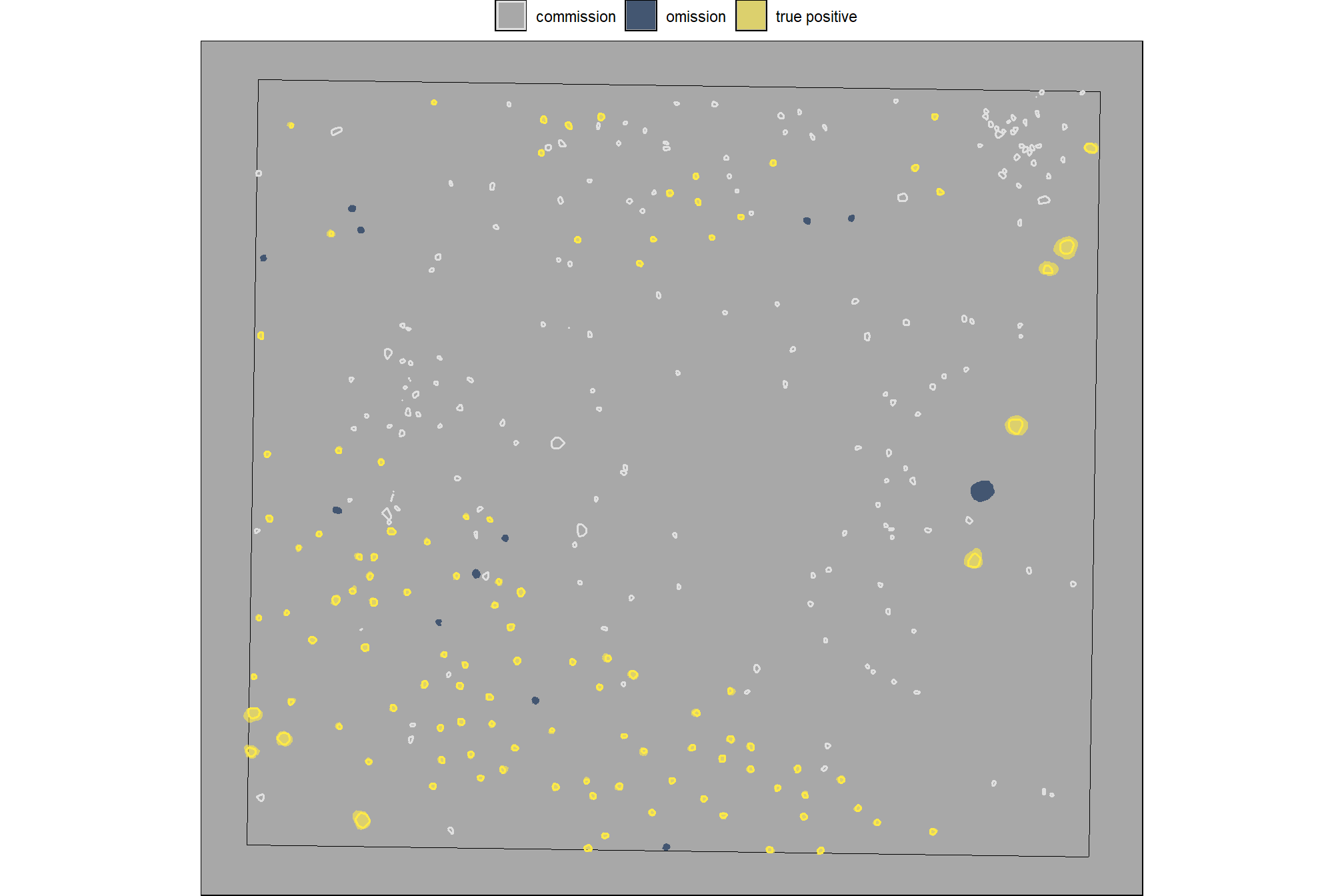
how do the area and volume metrics look?
p1_temp <- slash_pile_detect_watershed_ans_temp %>%
  ggplot2::ggplot() +
  ggplot2::geom_sf(mapping = ggplot2::aes(fill = area_m2)) +
  ggplot2::scale_fill_distiller(palette = "Blues", direction = 1) +
  ggplot2::labs(x="",y="") +
  ggplot2::theme_light() +
  ggplot2::theme(legend.position = "top", axis.text = ggplot2::element_blank())
p2_temp <- slash_pile_detect_watershed_ans_temp %>%
  ggplot2::ggplot() +
  ggplot2::geom_sf(mapping = ggplot2::aes(fill = volume_m3)) +
  ggplot2::scale_fill_distiller(palette = "BuGn", direction = 1) +
  ggplot2::labs(x="",y="") +
  ggplot2::theme_light() +
  ggplot2::theme(legend.position = "top", axis.text = ggplot2::element_blank())
p3_temp <- slash_pile_detect_watershed_ans_temp %>%
  ggplot2::ggplot() +
  ggplot2::geom_sf(mapping = ggplot2::aes(fill = max_height_m)) +
  ggplot2::scale_fill_distiller(palette = "YlOrBr", direction = 1) +
  ggplot2::labs(x="",y="") +
  ggplot2::theme_light() +
  ggplot2::theme(legend.position = "top", axis.text = ggplot2::element_blank())
p4_temp <- slash_pile_detect_watershed_ans_temp %>%
  ggplot2::ggplot() +
  ggplot2::geom_sf(mapping = ggplot2::aes(fill = diameter_m)) +
  ggplot2::scale_fill_distiller(palette = "PuRd", direction = 1) +
  ggplot2::labs(x="",y="") +
  ggplot2::theme_light() +
  ggplot2::theme(legend.position = "top", axis.text = ggplot2::element_blank())
(p1_temp + p2_temp) / (p3_temp + p4_temp)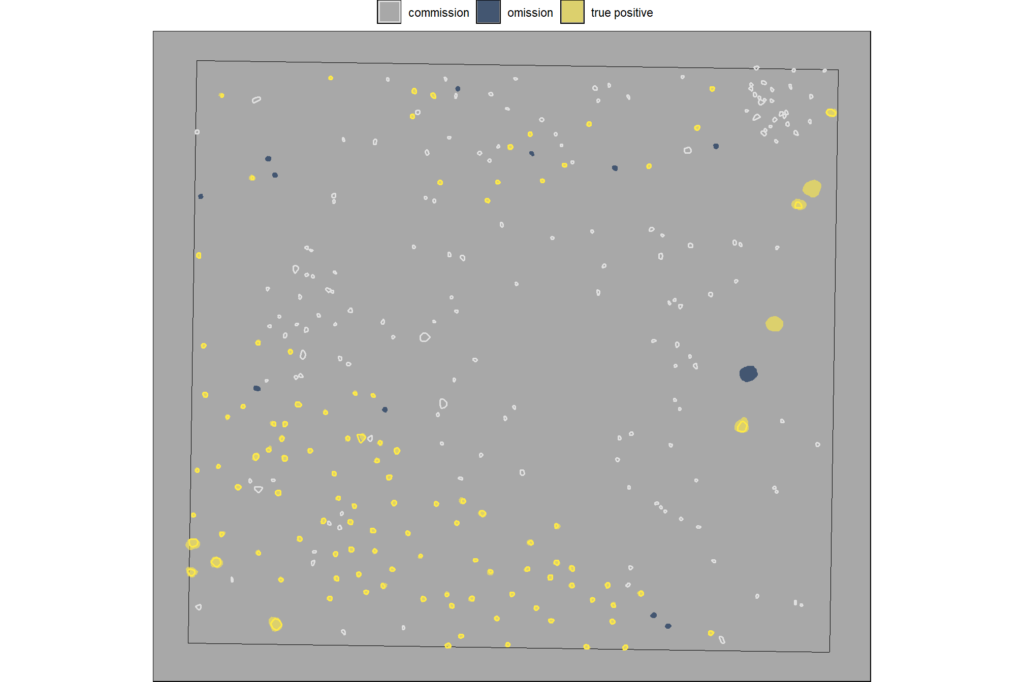
the volume per area ratio (volume_per_area) quantifies the “effective” height or depth of that volume relative to the area it occupies; this ratio may not be very useful for anything other than scaling estimates to relate a three-dimensional quantity (volume) to a two-dimensional quantity (area)
6.2 Parameter sensitivity testing
Parameter sensitivity testing is a systematic process of evaluating how changes to the specific thresholds and settings within the detection methodology impact the final results. Since the method doesn’t use training data, its performance is highly dependent on these manually defined parameters. The objective of this testing is to understand the robustness of the method and identify the optimal combination of settings that yield the best detection performance, balancing factors like detection rate (recall) and accuracy of positive predictions (precision).
Here are the general steps to accomplish this testing:
- Define Parameter Ranges and Increments: For each identified parameter, determine a reasonable range of values to test and the step size for incrementing through that range. For example, if a threshold is currently 0.5, you might test from 0.3 to 0.7 in increments of 0.05.
- Automate the Detection Workflow: Create a script or automated process that can run your entire rules-based slash pile detection method using different combinations of these parameter values.
- Execute Tests: Run the automated workflow for each defined parameter combination.
- Collect Performance Metrics: For every run, calculate the key performance metrics against your image-annotated validation data (e.g. recall, precision, F-score)
- Analyze and Visualize Results: Plot the performance metrics against the varying parameter values or combinations. This will help you visualize trends, identify sweet spots where performance is maximized, and understand trade-offs (e.g., increasing recall might decrease precision).
- Select Optimal Parameters: Based on the analysis and the specific goals of the project (e.g., minimizing false negatives for safety, or maximizing overall accuracy), select the parameter set that provides the most desirable performance. This might involve choosing a balance between precision and recall, or prioritizing one over the other.
param_combos_df <-
  tidyr::crossing(
    max_ht_m = seq(from = 2, to =  5, by = 1) # set the max expected pile height (could also do a minimum??)
    , min_area_m2 = c(2) # seq(from = 1, to =  2, by = 1) # set the min expected pile area
    , max_area_m2 = seq(from = 10, to =  100, by = 10) # set the max expected pile area
    , convexity_pct = seq(from = 0.3, to =  0.8, by = 0.1) # min required overlap between the predicted pile and the convex hull of the predicted pile
    , circle_fit_iou_pct = seq(from = 0.3, to = 0.8, by = 0.1)
  ) %>%
  dplyr::mutate(rn = dplyr::row_number()) %>%
  dplyr::relocate(rn)
# huh?
param_combos_df %>% dplyr::glimpse()
## Rows: 1,440
## Columns: 6
## $ rn <int> 1, 2, 3, 4, 5, 6, 7, 8, 9, 10, 11, 12, 13, 14, 15, …
## $ max_ht_m <dbl> 2, 2, 2, 2, 2, 2, 2, 2, 2, 2, 2, 2, 2, 2, 2, 2, 2, …
## $ min_area_m2 <dbl> 2, 2, 2, 2, 2, 2, 2, 2, 2, 2, 2, 2, 2, 2, 2, 2, 2, …
## $ max_area_m2 <dbl> 10, 10, 10, 10, 10, 10, 10, 10, 10, 10, 10, 10, 10,…
## $ convexity_pct <dbl> 0.3, 0.3, 0.3, 0.3, 0.3, 0.3, 0.4, 0.4, 0.4, 0.4, 0…
## $ circle_fit_iou_pct <dbl> 0.3, 0.4, 0.5, 0.6, 0.7, 0.8, 0.3, 0.4, 0.5, 0.6, 0…that might be too many combinations but we’ll give it a shot
6.2.1 Workflow over parameter combinations
to automate the detection workflow we can simply map these combinations over our slash_pile_detect_watershed() function. however, that would result in us running the same watershed segmentation process repeatedly with the same settings. as such, let’s make a function to efficiently perform the detection workflow using the same watershed segmentation and circle fitting for use with the different filtering combinations.
#########################################################################
# 1)
# function to apply watershed seg over a list of max_ht_m
# function to apply watershed segmentation over a list of different maximum height threshold (`max_ht_m`) which determines the "slice" of the CHM to use
#########################################################################
chm_watershed_seg_fn <- function(chm_rast,max_ht_m) {
# get unique hts
max_ht_m <- unique(as.numeric(max_ht_m))
max_ht_m <- max_ht_m[!is.na(max_ht_m)]
if(
dplyr::coalesce(length(max_ht_m),0)<1
){stop("could not detect `max_ht_m` parameter setting which should be numeric list")}
# checks
if(!inherits(chm_rast,"SpatRaster")){stop("`chm_rast` must be raster data with the class `SpatRaster` ")}
# just get the first layer
chm_rast <- chm_rast %>% terra::subset(subset = 1)
# # first, calculate the area of each cell
# area_rast <- terra::cellSize(chm_rast)
# names(area_rast) <- "area_m2"
# map over the max_ht_m to get the raster slice
chm_ret_rast <- max_ht_m %>%
purrr::map(\(x)
terra::clamp(chm_rast, upper = x, lower = 0, values = F)
) %>%
terra::rast()
# name
names(chm_ret_rast) <- as.character(max_ht_m)
# chm_ret_rast
# chm_ret_rast %>% terra::subset(1) %>% terra::plot()
# chm_ret_rast %>% terra::subset(2) %>% terra::plot()
# chm_rast[[1]]
# # map over the volume
# # then, multiply area by the CHM (elevation) for each cell to get a raster with cell volumes
# vol_ret_rast <-
# 1:terra::nlyr(chm_ret_rast) %>%
# purrr::map(function(x){
# vol_rast <- area_rast*chm_ret_rast[[x]]
# names(vol_rast) <- "volume_m3"
# return(vol_rast)
# }) %>%
# terra::rast()
# # name
# names(vol_ret_rast) <- as.character(max_ht_m)
# map over the watershed
# let's run watershed segmentation using `lidR::watershed()` which is based on the bioconductor package `EBIimage`
# return is a raster with the first layer representing the identified watershed segments
ret_rast <-
1:terra::nlyr(chm_ret_rast) %>%
purrr::map(\(x)
lidR::watershed(
chm = chm_ret_rast[[x]]
, th_tree = 0.5 # this would be the minimum expected pile height
)()
) %>%
terra::rast()
# name
names(ret_rast) <- as.character(max_ht_m)
# ret_rast
# ret_rast %>% terra::subset(1) %>% terra::as.factor() %>% terra::plot()
# ret_rast %>% terra::subset(2) %>% terra::as.factor() %>% terra::plot()
return(list(
chm_rast = chm_ret_rast # length = length(max_ht_m)
# , area_rast = area_rast # length = 1
# , volume_rast = vol_ret_rast # length = length(max_ht_m)
, watershed_rast = ret_rast # length = length(max_ht_m)
))
}
# xxx <- chm_watershed_seg_fn(
# cloud2raster_ans$chm_rast %>%
# terra::crop(
# stand_boundary %>%
# dplyr::slice(1) %>%
# sf::st_buffer(-80) %>%
# sf::st_transform(terra::crs(cloud2raster_ans$chm_rast)) %>%
# terra::vect()
# )
# ,c(4,5)
# )
# xxx$chm_rast %>% terra::subset( as.character(unique(c(4,5))[1]) ) %>% terra::plot()
# xxx$watershed_rast %>% terra::subset( as.character(unique(c(4,5))[1]) ) %>% terra::as.factor() %>% terra::plot()
# # xxx$volume_rast %>% terra::subset( as.character(unique(c(4,5))[1]) ) %>% terra::plot()
# # xxx$area_rast[[1]] %>% terra::minmax()
# # xxx$area_rast %>% terra::plot()
#########################################################################
# 2)
# now we need to define a function to apply the filters to the resulting watershed segmented rasters
# based on a data frame of difference combinations of filters for irregularity using the comparison to the convex hull
#########################################################################
param_combos_detect_convexity_fn <- function(
chm_watershed_seg_fn_ans
#### height and area thresholds for the detected piles
# these should be based on data from the literature or expectations based on the prescription
, max_ht_m = 4 # set the max expected pile height (could also do a minimum??)
#### irregularity filtering
# 1 = perfectly convex (no inward angles); 0 = so many inward angles
# values closer to 1 remove more irregular segments;
# values closer to 0 keep more irregular segments (and also regular segments)
# these will all be further filtered for their circularity and later smoothed to remove blocky edges
# and most inward angles by applying a convex hull to the original detected segment
, convexity_pct = 0.7 # min required overlap between the predicted pile and the convex hull of the predicted pile
) {
# extract individual elements from chm_watershed_seg_fn
chm_rast <- chm_watershed_seg_fn_ans$chm_rast %>% terra::subset( as.character(unique(max_ht_m)[1]) )
watershed_ans <- chm_watershed_seg_fn_ans$watershed_rast %>% terra::subset( as.character(unique(max_ht_m)[1]) )
names(watershed_ans) <- "pred_id"
# checks
if(!inherits(chm_rast,"SpatRaster")){stop("`chm_rast` must be raster data with the class `SpatRaster` ")}
if(!inherits(watershed_ans,"SpatRaster")){stop("`watershed_ans` must be raster data with the class `SpatRaster` ")}
########################################################################################
## convert to polys and area filters
########################################################################################
# let's convert the watershed-detected segments from raster to vector data
# and create a convex hull of the shapes for comparison
# vectors of segments
watershed_ans_poly <-
watershed_ans %>%
terra::as.polygons(round = F, aggregate = T, values = T, extent = F, na.rm = T) %>%
sf::st_as_sf() %>%
sf::st_simplify() %>%
sf::st_make_valid() %>%
dplyr::filter(sf::st_is_valid(.)) %>%
dplyr::mutate(treeID=pred_id) %>%
cloud2trees::simplify_multipolygon_crowns() %>%
dplyr::select(-treeID)
if(dplyr::coalesce(nrow(watershed_ans_poly),0)<1){
return(NULL)
}
########################################################################################
## 2) irregularity filtering
########################################################################################
# let's first filter out segments that have holes in them
# or are very irregularly shaped by comparing the area of the polygon and convex hull
# convexity_pct = min required overlap between the predicted pile and the convex hull of the predicted pile
if(convexity_pct>0){
# apply the irregularity filtering on the polygons
watershed_ans_poly <- watershed_ans_poly %>%
st_irregular_remove(pct_chull_overlap = convexity_pct)
}
if(dplyr::coalesce(nrow(watershed_ans_poly),0)==0){
return(NULL)
}else{
return(watershed_ans_poly %>% dplyr::mutate(max_ht_m = max_ht_m, convexity_pct = convexity_pct))
}
}
# # just get the unique combinations needed for this param_combos_detect_convexity_fn function
# param_combos_convexity_df <-
# param_combos_df %>%
# dplyr::filter(max_ht_m %in% as.numeric(names(xxx$chm_rast))) %>% ## !!!!!!!!!!take this out
# dplyr::distinct(max_ht_m,convexity_pct)
# # apply this using our data frame to map over the combinations
# ### takes ~40 mins
# param_combos_detect_convexity_ans <-
# 1:nrow(param_combos_convexity_df) %>%
# sample(2) %>%
# purrr::map(\(x)
# param_combos_detect_convexity_fn(
# chm_watershed_seg_fn_ans = xxx ## !!!!!!!!!!change this
# , max_ht_m = param_combos_convexity_df$max_ht_m[x]
# , convexity_pct = param_combos_convexity_df$convexity_pct[x]
# )
# , .progress = T
# ) %>%
# dplyr::bind_rows()
# # param_combos_detect_convexity_ans %>% dplyr::glimpse()
# # param_combos_detect_convexity_ans %>% sf::st_drop_geometry() %>% dplyr::count(max_ht_m,convexity_pct)
# # param_combos_detect_convexity_ans %>%
# # dplyr::mutate(area_xxxx = sf::st_area(.) %>% as.numeric()) %>%
# # sf::st_drop_geometry() %>%
# # dplyr::group_by(max_ht_m,convexity_pct) %>%
# # dplyr::summarise(dplyr::across(area_xxxx, list(min = min, max = max), .names = "{.col}.{.fn}"))
#
# # now just join to filter for area
# # expands to row unique by max_ht_m,convexity_pct,min_area_m2,max_area_m2,pred_id
# param_combos_area <-
# param_combos_detect_convexity_ans %>%
# dplyr::mutate(area_xxxx = sf::st_area(.) %>% as.numeric()) %>%
# dplyr::inner_join(
# # add area ranges
# param_combos_df %>%
# dplyr::distinct(max_ht_m,convexity_pct,min_area_m2,max_area_m2)
# , by = dplyr::join_by(
# max_ht_m, convexity_pct
# , area_xxxx>=min_area_m2
# , area_xxxx<=max_area_m2
# )
# , relationship = "many-to-many"
# )
# # dplyr::filter(
# # area_xxxx>=min_area_m2
# # , area_xxxx<=max_area_m2
# # )
# param_combos_area %>% dplyr::glimpse()
# param_combos_area %>%
# sf::st_drop_geometry() %>%
# dplyr::group_by(max_ht_m,convexity_pct,min_area_m2,max_area_m2) %>%
# dplyr::summarise(dplyr::across(area_xxxx, list(min = min, max = max), .names = "{.col}.{.fn}"))
#
# # geometries are unique by max_ht_m,pred_id
# param_combos_area %>%
# dplyr::filter(
# pred_id == param_combos_area$pred_id[111]
# , max_ht_m == param_combos_area$max_ht_m[111]
# ) %>%
# dplyr::mutate(lab = stringr::str_c(max_ht_m,convexity_pct,min_area_m2,max_area_m2, sep = ":")) %>%
# ggplot() + geom_sf(aes(linetype = lab, color = lab),fill=NA) + facet_wrap(facets = dplyr::vars(lab)) + theme_void()
# param_combos_area %>%
# dplyr::group_by(max_ht_m,pred_id) %>%
# dplyr::filter(dplyr::row_number()==1) %>%
# dplyr::select(max_ht_m,pred_id) %>%
# dplyr::ungroup() %>%
# # dplyr::glimpse()
# ggplot() + geom_sf(aes(color = factor(max_ht_m)),fill=NA) + facet_wrap(facets = dplyr::vars(max_ht_m))
# unique_geometries_cf <- sf_data_circle_fit(
# param_combos_area %>%
# dplyr::group_by(max_ht_m,pred_id) %>%
# dplyr::filter(dplyr::row_number()==1) %>%
# dplyr::select(max_ht_m,pred_id) %>%
# dplyr::ungroup()
# )
# unique_geometries_cf %>% dplyr::glimpse()
# function to smooth
raster_smooth_smoother <- function(
chm_watershed_seg_fn_ans
, max_ht_m = 4
, watershed_ans_poly
, min_area_m2 = 2
) {
# extract individual elements from chm_watershed_seg_fn
chm_rast <- chm_watershed_seg_fn_ans$chm_rast %>% terra::subset( as.character(unique(max_ht_m)[1]) )
watershed_ans <- chm_watershed_seg_fn_ans$watershed_rast %>% terra::subset( as.character(unique(max_ht_m)[1]) )
names(watershed_ans) <- "pred_id"
# checks
if(!inherits(chm_rast,"SpatRaster")){stop("`chm_rast` must be raster data with the class `SpatRaster` ")}
if(!inherits(watershed_ans,"SpatRaster")){stop("`watershed_ans` must be raster data with the class `SpatRaster` ")}
chm_res <- max(terra::res(chm_rast)[1:2],na.rm = T)
ws_for_smooth <- ws_for_smooth_fn(chm_res = chm_res, min_area_m2 = min_area_m2) # 3 # needs to be the same for the watershed seg and CHM smooth
# search_area = (res^2) * (ws^2)
########################################################################################
## 5) raster smoothing
########################################################################################
########################################
# use the remaining segments that meet the geometric and area filtering
# to smooth the watershed raster
########################################
smooth_watershed_ans <- watershed_ans %>%
terra::mask(
watershed_ans_poly %>% #these are irregularity and area filtered already
terra::vect()
, updatevalue=NA
)
if(dplyr::coalesce(ws_for_smooth,0)>=3){
# smooths the raster using the majority value
smooth_watershed_ans <- smooth_watershed_ans %>%
terra::focal(w = ws_for_smooth, fun = "modal", na.rm = T, na.policy = "only") # only fill NA cells
}
names(smooth_watershed_ans) <- "pred_id"
########################################
# mask the chm rast to these remaining segments and smooth to match the smoothing for the segments
########################################
smooth_chm_rast <- chm_rast %>%
terra::mask(smooth_watershed_ans)
if(dplyr::coalesce(ws_for_smooth,0)>=3){
# smooths the raster to match the smoothing in the watershed segments
smooth_chm_rast <- smooth_chm_rast %>%
terra::focal(w = ws_for_smooth, fun = "mean", na.rm = T, na.policy = "only") #only for cells that are NA
}
# now mask the watershed_ans raster to only keep cells that are in the originating CHM
smooth_watershed_ans <- smooth_watershed_ans %>%
terra::mask(smooth_chm_rast)
########################################################################################
## calculate raster-based area and volume
########################################################################################
# first, calculate the area of each cell
area_rast <- terra::cellSize(smooth_chm_rast)
names(area_rast) <- "area_m2"
# area_rast %>% terra::plot()
# then, multiply area by the CHM (elevation) for each cell to get a raster with cell volumes
vol_rast <- area_rast*smooth_chm_rast
names(vol_rast) <- "volume_m3"
# vol_rast %>% terra::plot()
# sum area within each segment to get the total area
area_df <- terra::zonal(x = area_rast, z = smooth_watershed_ans, fun = "sum", na.rm = T)
# sum volume within each segment to get the total volume
vol_df <- terra::zonal(x = vol_rast, z = smooth_watershed_ans, fun = "sum", na.rm = T)
# max ht within each segment to get the max ht
ht_df <- terra::zonal(x = smooth_chm_rast, z = smooth_watershed_ans, fun = "max", na.rm = T) %>%
dplyr::rename(max_height_m=2)
# let's convert the smoothed and filtered watershed-detected segments from raster to vector data
# vectors of segments
watershed_ans_poly <-
smooth_watershed_ans %>%
terra::as.polygons(round = F, aggregate = T, values = T, extent = F, na.rm = T) %>%
sf::st_as_sf() %>%
sf::st_simplify() %>%
sf::st_make_valid() %>%
dplyr::filter(sf::st_is_valid(.)) %>%
dplyr::mutate(treeID=pred_id) %>%
cloud2trees::simplify_multipolygon_crowns() %>%
dplyr::select(-treeID)
# add area and volume to our vector data
# we'll do this with a slick trick to perform multiple joins succinctly using purrr::reduce
watershed_ans_poly <-
purrr::reduce(
list(watershed_ans_poly, area_df, vol_df, ht_df)
, dplyr::left_join
, by = 'pred_id'
) %>%
dplyr::mutate(
volume_per_area = volume_m3/area_m2
)
# # filter out the segments that don't meet the size thresholds
# dplyr::filter(
# dplyr::coalesce(area_m2,0) >= min_area_m2
# & dplyr::coalesce(area_m2,0) <= max_area_m2
# ) %>%
# # do one more pass of the irregularity filtering
# st_irregular_remove(pct_chull_overlap = convexity_pct)
if(dplyr::coalesce(nrow(watershed_ans_poly),0)==0){
return(NULL)
}else{
return(watershed_ans_poly)
}
}
# param_combos_piles %>% dplyr::slice_head(n=222) %>%
# # sf::st_geometry() %>%
# sf::st_set_geometry("geometry") %>%
# dplyr::slice(1:3) %>%
# dplyr::rowwise() %>%
# dplyr::mutate(diam = st_calculate_diameter(geometry)) %>%
# dplyr::ungroup() %>%
# dplyr::glimpse()
# function to do the whole thing
param_combos_piles_detect_fn <- function(
chm
, param_combos_df
, smooth_segs = T
, ofile = "../data/param_combos_piles.gpkg"
) {
########################################################################################
## 1) chm slice and watershed segmentation
########################################################################################
# apply chm_watershed_seg_fn
### takes ~37 mins
chm_watershed_seg_ans <- chm_watershed_seg_fn(chm, max_ht_m = unique(param_combos_df$max_ht_m))
# # what did we get?
# chm_watershed_seg_ans %>%
# terra::subset( as.character(unique(param_combos_df$max_ht_m)[3]) ) %>%
# terra::plot()
########################################################################################
## 2) irregularity filter
########################################################################################
# just get the unique combinations needed for this param_combos_detect_convexity_fn function
param_combos_convexity_df <-
param_combos_df %>%
dplyr::distinct(max_ht_m,convexity_pct)
# apply this using our data frame to map over the combinations
### takes ~40 mins
param_combos_detect_convexity_ans <-
1:nrow(param_combos_convexity_df) %>%
purrr::map(\(x)
param_combos_detect_convexity_fn(
chm_watershed_seg_fn_ans = chm_watershed_seg_ans
, max_ht_m = param_combos_convexity_df$max_ht_m[x]
, convexity_pct = param_combos_convexity_df$convexity_pct[x]
)
, .progress = "convexity filtering"
) %>%
dplyr::bind_rows()
# param_combos_detect_convexity_ans %>% dplyr::glimpse()
# param_combos_detect_convexity_ans %>% sf::st_drop_geometry() %>% dplyr::count(max_ht_m,convexity_pct)
# param_combos_detect_convexity_ans %>%
# dplyr::mutate(area_xxxx = sf::st_area(.) %>% as.numeric()) %>%
# sf::st_drop_geometry() %>%
# dplyr::group_by(max_ht_m,convexity_pct) %>%
# dplyr::summarise(dplyr::across(area_xxxx, list(min = min, max = max), .names = "{.col}.{.fn}"))
########################################################################################
## 3) area filter
########################################################################################
# now just join to filter for area
# expands to row unique by max_ht_m,convexity_pct,min_area_m2,max_area_m2,pred_id
param_combos_area <-
param_combos_detect_convexity_ans %>%
dplyr::mutate(area_xxxx = sf::st_area(.) %>% as.numeric()) %>%
dplyr::inner_join(
# add area ranges
param_combos_df %>%
dplyr::distinct(max_ht_m,convexity_pct,min_area_m2,max_area_m2)
, by = dplyr::join_by(
max_ht_m, convexity_pct
, area_xxxx>=min_area_m2
, area_xxxx<=max_area_m2
)
, relationship = "many-to-many"
) %>%
dplyr::select(-area_xxxx)
# dplyr::filter(
# area_xxxx>=min_area_m2
# , area_xxxx<=max_area_m2
# )
# param_combos_area %>% dplyr::glimpse()
# param_combos_area %>%
# sf::st_drop_geometry() %>%
# dplyr::group_by(max_ht_m,convexity_pct,min_area_m2,max_area_m2) %>%
# dplyr::summarise(dplyr::across(area_xxxx, list(min = min, max = max), .names = "{.col}.{.fn}"))
# !!!!!!!!!!!!!!!!!!!!!!geometries are unique by max_ht_m,pred_id!!!!!!!!!!!!!!!!!!!!!!
# param_combos_area %>%
# dplyr::filter(
# pred_id == param_combos_area$pred_id[111]
# , max_ht_m == param_combos_area$max_ht_m[111]
# ) %>%
# dplyr::mutate(lab = stringr::str_c(max_ht_m,convexity_pct,min_area_m2,max_area_m2, sep = ":")) %>%
# ggplot() + geom_sf(aes(linetype = lab, color = lab),fill=NA) + facet_wrap(facets = dplyr::vars(lab)) + theme_void()
# param_combos_area %>%
# dplyr::group_by(max_ht_m,pred_id) %>%
# dplyr::filter(dplyr::row_number()==1) %>%
# dplyr::select(max_ht_m,pred_id) %>%
# dplyr::ungroup() %>%
# # dplyr::glimpse()
# ggplot() + geom_sf(aes(color = factor(max_ht_m)),fill=NA) + facet_wrap(facets = dplyr::vars(max_ht_m))
########################################################################################
## 4) circle filter
########################################################################################
# !!!!!!!!!!!!!!!!!!!!!!geometries are unique by max_ht_m,pred_id!!!!!!!!!!!!!!!!!!!!!!
unique_geometries <- param_combos_area %>%
dplyr::group_by(max_ht_m,pred_id) %>%
dplyr::filter(dplyr::row_number()==1) %>%
dplyr::ungroup() %>%
dplyr::select(max_ht_m,pred_id) %>%
dplyr::mutate(record_id = dplyr::row_number())
# param_combos_detect_convexity_ans %>% dplyr::glimpse()
# and we'll apply the circle fitting to this spatial data
# apply the sf_data_circle_fit() which takes each segment polygon, transforms it to points, and the fits the best circle
unique_geometries_cf <- sf_data_circle_fit(unique_geometries)
# param_combos_detect_cf_ans %>% sf::st_write("../data/param_combos_detect_cf_ans.gpkg")
# param_combos_detect_cf_ans %>% dplyr::glimpse()
# nrow(param_combos_detect_cf_ans)
# nrow(param_combos_detect_convexity_ans)
# we'll use the IoU function we defined
# we map over this to only compare the segment to it's own best circle fit...not all
# we should consider doing this in bulk.....another day
param_combos_detect_cf_iou <-
unique_geometries$record_id %>%
purrr::map(\(x)
ground_truth_single_match(
gt_inst = unique_geometries %>%
dplyr::filter(record_id == x)
, gt_id = "record_id"
, predictions = unique_geometries_cf %>%
dplyr::filter(record_id == x) %>%
dplyr::select(record_id) %>% # keeping other columns causes error?
dplyr::rename(circ_record_id = record_id)
, pred_id = "circ_record_id"
, min_iou_pct = 0 # set to 0 just to return pct
)
) %>%
dplyr::bind_rows()
# param_combos_detect_cf_iou %>% dplyr::glimpse()
### now we need a function to map over all the different filters for circularity by combination of the other settings
### this is going to be highly custom to this particular task :\
param_combos_circle_fit <-
param_combos_area %>%
# expands row to unique by max_ht_m,min_area_m2,max_area_m2,convexity_pct,circle_fit_iou_pct,pred_id
dplyr::inner_join(
param_combos_df
, by = dplyr::join_by(max_ht_m,min_area_m2,max_area_m2,convexity_pct)
, relationship = "many-to-many"
) %>%
# join unique geoms
dplyr::inner_join(
unique_geometries %>%
sf::st_drop_geometry() %>%
dplyr::select(max_ht_m,pred_id,record_id)
, by = dplyr::join_by(max_ht_m,pred_id)
) %>%
# join circle fits
dplyr::left_join(
param_combos_detect_cf_iou %>% dplyr::select(record_id,iou)
, by = "record_id"
) %>%
dplyr::filter(dplyr::coalesce(iou,0)>=circle_fit_iou_pct)
############################################################
# get unique sets of pred_id by height so we only need to smooth the raster for these sets
############################################################
rn_geom_lookup <- param_combos_circle_fit %>%
sf::st_drop_geometry() %>%
dplyr::arrange(rn,max_ht_m,pred_id) %>%
dplyr::group_by(rn,max_ht_m) %>%
dplyr::summarise(preds = paste(sort(pred_id), collapse = "_"),n=dplyr::n()) %>%
dplyr::ungroup() %>%
dplyr::arrange(max_ht_m,desc(n))
# now just get the unique sets by max_ht_m
rn_geom_lookup <- rn_geom_lookup %>%
dplyr::inner_join(
rn_geom_lookup %>%
dplyr::distinct(max_ht_m,preds) %>%
dplyr::mutate(set_id = dplyr::row_number())
, by = dplyr::join_by(max_ht_m,preds)
) %>%
dplyr::select(set_id,rn,max_ht_m)
# rn_geom_lookup %>% dplyr::glimpse()
# now just get the unique max_ht_m and actual geoms
geom_sets <-
param_combos_circle_fit %>%
dplyr::select(rn,max_ht_m,pred_id) %>%
dplyr::inner_join(
rn_geom_lookup %>%
dplyr::group_by(set_id) %>%
dplyr::filter(dplyr::row_number()==1) %>%
dplyr::ungroup() %>%
dplyr::select(rn,set_id)
, by = dplyr::join_by(rn)
)
# dplyr::relocate(set_id) %>%
# dplyr::arrange(set_id,pred_id) %>%
# dplyr::glimpse()
########
########################################################################################
## 6) raster smooth
########################################################################################
geom_sets_smooth <-
geom_sets$set_id %>%
unique() %>%
purrr::map(\(x)
raster_smooth_smoother(
chm_watershed_seg_fn_ans = chm_watershed_seg_ans
, max_ht_m = (geom_sets %>% sf::st_drop_geometry() %>% dplyr::filter(set_id==x) %>% dplyr::slice(1) %>% dplyr::pull(max_ht_m))
, watershed_ans_poly = geom_sets %>% dplyr::filter(set_id==x)
, min_area_m2 = min(param_combos_df$min_area_m2,na.rm=T) ##### this fixes the parameter
# .......... so won't work if param_combos_df contains multiple values #ohwell...just don't test min_area_m2
) %>%
dplyr::mutate(
set_id = x
, max_ht_m = (geom_sets %>% sf::st_drop_geometry() %>% dplyr::filter(set_id==x) %>% dplyr::slice(1) %>% dplyr::pull(max_ht_m))
)
, .progress = "smooth smoothing it"
) %>%
dplyr::bind_rows()
# geom_sets_smooth %>% dplyr::glimpse()
# ggplot() +
# geom_sf(
# data = geom_sets_smooth %>% dplyr::filter(set_id == geom_sets_smooth$set_id[1])
# , fill = "navy"
# , alpha = 0.8
# ) +
# geom_sf(
# data = geom_sets %>% dplyr::filter(set_id == geom_sets_smooth$set_id[1])
# , fill = NA
# , color = "gold"
# ) +
# theme_void()
# # these polygons are unique
# # diameter
# message("diametering.....")
# geom_sets_smooth <- geom_sets_smooth %>%
# sf::st_set_geometry("geometry") %>%
# dplyr::rowwise() %>%
# dplyr::mutate(diameter_m = st_calculate_diameter(geometry)) %>%
# dplyr::ungroup()
########################################################################################
## 6.3) second irregular filter
########################################################################################
# get set, convexity combinations to map over st_irregular_remove
set_convexity_combo <-
rn_geom_lookup %>%
# add in convexity pct to get unique set_id, convexity
dplyr::inner_join(
param_combos_df %>%
dplyr::select(rn,convexity_pct)
, by = "rn"
) %>%
dplyr::distinct(set_id,convexity_pct)
# filter for convexity
geom_sets_convexity <-
1:nrow(set_convexity_combo) %>%
purrr::map(\(x)
st_irregular_remove(
sf_data = geom_sets_smooth %>% dplyr::filter(set_id==set_convexity_combo$set_id[x])
, pct_chull_overlap = set_convexity_combo$convexity_pct[x]
) %>%
dplyr::mutate(
set_id = set_convexity_combo$set_id[x]
, convexity_pct = set_convexity_combo$convexity_pct[x]
)
, .progress = "second irregularity filter"
) %>%
dplyr::bind_rows()
# row is unique by set_id,convexity_pct,pred_id
# geom_sets_convexity %>% dplyr::glimpse()
# geom_sets_convexity %>% sf::st_drop_geometry() %>% dplyr::count(set_id,convexity_pct)
########################################################################################
## 6.6) second area filter
########################################################################################
# filter for area
message("expanding to final param combos.....")
filtered_final <-
geom_sets_convexity %>%
dplyr::select(-c(max_ht_m)) %>%
# expand to full param_combos_df
dplyr::inner_join(
param_combos_df %>%
dplyr::inner_join(
rn_geom_lookup %>% dplyr::select(rn,set_id)
, by = "rn"
)
, by = dplyr::join_by(set_id,convexity_pct)
, relationship = "many-to-many"
) %>%
# filter for area
dplyr::filter(
dplyr::coalesce(area_m2,0) >= min_area_m2
& dplyr::coalesce(area_m2,0) <= max_area_m2
) %>%
dplyr::select(-c(set_id)) %>%
dplyr::relocate(names(param_combos_df))
# filtered_final %>% dplyr::glimpse()
########################################################################################
## 7) shape refinement & overlap removal
########################################################################################
# use the convex hull shapes of our remaining segments.
# This helps to smooth out the often 'blocky' edges of raster-based segments
# , which can look like they were generated in Minecraft.
# Additionally, by removing any segments with overlapping convex hull shapes,
# we can likely reduce false detections that are actually groups of small trees or shrubs,
# ensuring our results represent singular slash piles.
smooth_segs <- T
if(smooth_segs){
# smooth unique polygons
message("shape refinement and diametering.....")
##### just work with unique polygons
##### geom_sets_smooth row is unique by: set_id,pred_id
geom_sets_final <- geom_sets_smooth %>%
dplyr::select( -dplyr::any_of(c(
"hey_xxxxxxxxxx"
, "max_ht_m"
))) %>%
# join to filter geoms
dplyr::inner_join(
rn_geom_lookup %>%
dplyr::inner_join(
filtered_final %>%
sf::st_drop_geometry() %>%
dplyr::distinct(rn,pred_id)
, by = dplyr::join_by(rn)
, relationship = "one-to-many"
) %>%
# just get the unique geoms now
dplyr::distinct(set_id,pred_id)
, by = dplyr::join_by(set_id,pred_id)
, relationship = "one-to-one"
) %>%
# smooth
sf::st_convex_hull() %>%
sf::st_simplify() %>%
sf::st_make_valid() %>%
dplyr::filter(sf::st_is_valid(.)) %>%
# diameter
sf::st_set_geometry("geometry") %>%
dplyr::rowwise() %>%
dplyr::mutate(diameter_m = st_calculate_diameter(geometry)) %>%
dplyr::ungroup() %>%
# now we need to re-do the volume and area calculations
dplyr::mutate(
area_m2 = sf::st_area(.) %>% as.numeric()
, volume_m3 = area_m2*volume_per_area
)
# ##### geom_sets_final row is unique by: set_id,pred_id
# geom_sets_final %>% dplyr::glimpse()
# ggplot() +
# geom_sf(
# # post smooth (should be slightly larger)
# data = geom_sets_final %>% dplyr::filter(set_id == geom_sets_final$set_id[1])
# , fill = "navy"
# , alpha = 0.8
# , color = "gray"
# , lwd = 0.2
# ) +
# theme_void()
# ggplot() +
# geom_sf(
# # post smooth (should be slightly larger)
# data = geom_sets_final %>% dplyr::filter(set_id == geom_sets_final$set_id[1])
# , fill = "navy"
# , alpha = 0.8
# , color = "gray"
# , lwd = 0.2
# ) +
# geom_sf(
# # pre-smooth
# data = geom_sets %>% dplyr::filter(set_id == geom_sets_final$set_id[1])
# , fill = NA
# , color = "gold"
# ) +
# theme_void()
# sf::st_read("c:/data/usfs/manitou_slash_piles/data/param_combos_piles_chm0.45m.gpkg") %>%
# dplyr::mutate(xxxarea_m2 = sf::st_area(.) %>% as.numeric()) %>%
# sf::st_drop_geometry() %>%
# dplyr::slice_sample(n=33333) %>%
# ggplot2::ggplot(mapping = ggplot2::aes(x = xxxarea_m2, y =area_m2)) +
# ggplot2::geom_abline(lwd = 1) +
# ggplot2::geom_point() +
# ggplot2::geom_smooth(method = "lm", se=F, color = "tomato", linetype = "dashed") +
# ggplot2::scale_color_viridis_c(option = "mako", direction = -1, alpha = 0.8) +
# ggplot2::theme_light()
# ##### geom_sets_final row is unique by: set_id,pred_id
# overlapping convex hull shapes are then removed to prevent false positives from clustered small trees or shrubs
# have to map over this to do overlaps only on one set at a time
geom_sets_final_olaps <-
geom_sets_final$set_id %>%
unique() %>%
purrr::map(\(x)
geom_sets_final %>%
dplyr::filter(set_id==x) %>%
st_remove_overlaps()
) %>%
dplyr::bind_rows()
# ##### geom_sets_final_olaps row is unique by: set_id,pred_id
# geom_sets_final %>% dplyr::glimpse()
# geom_sets_final_olaps %>% dplyr::glimpse()
# ggplot() +
# geom_sf(
# # post smooth (should be slightly larger)
# data = geom_sets_final_olaps %>% dplyr::filter(set_id == geom_sets_final_olaps$set_id[1])
# , fill = "navy"
# , alpha = 0.8
# , color = "gray"
# , lwd = 0.2
# ) +
# geom_sf(
# # pre-smooth
# data = geom_sets_final %>% dplyr::filter(set_id == geom_sets_final_olaps$set_id[1])
# , fill = NA
# , color = "gold"
# , lwd = 1
# ) +
# theme_void()
# join back to param_combos list
final_ans <- geom_sets_final_olaps %>%
# join to lookup
# expands row to unique by set_id,rn,pred_id
dplyr::inner_join(
rn_geom_lookup %>%
dplyr::select(rn,set_id)
, by = dplyr::join_by(set_id)
, relationship = "many-to-many"
) %>%
# join with filtered_final which have pred_id
dplyr::inner_join(
filtered_final %>%
sf::st_drop_geometry() %>%
dplyr::distinct(rn,pred_id)
, by = dplyr::join_by(rn,pred_id)
, relationship = "one-to-one"
) %>%
# add param_combos_df data
dplyr::inner_join(
param_combos_df
, by = "rn"
, relationship = "many-to-one"
)
# nrow(filtered_final)
# nrow(final_ans) # should be less
}else{
message("diametering.....")
##### just work with unique polygons
##### geom_sets_smooth row is unique by: set_id,pred_id
geom_sets_final <- geom_sets_smooth %>%
dplyr::select( -dplyr::any_of(c(
"hey_xxxxxxxxxx"
, "max_ht_m"
))) %>%
# join to filter geoms
dplyr::inner_join(
rn_geom_lookup %>%
dplyr::inner_join(
filtered_final %>%
sf::st_drop_geometry() %>%
dplyr::distinct(rn,pred_id)
, by = dplyr::join_by(rn)
, relationship = "one-to-many"
) %>%
# just get the unique geoms now
dplyr::distinct(set_id,pred_id)
, by = dplyr::join_by(set_id,pred_id)
, relationship = "one-to-one"
) %>%
# diameter
sf::st_set_geometry("geometry") %>%
dplyr::rowwise() %>%
dplyr::mutate(diameter_m = st_calculate_diameter(geometry)) %>%
dplyr::ungroup()
# join back to param_combos list
final_ans <- geom_sets_final %>%
# join to lookup
# expands row to unique by set_id,rn,pred_id
dplyr::inner_join(
rn_geom_lookup %>%
dplyr::select(rn,set_id)
, by = dplyr::join_by(set_id)
, relationship = "many-to-many"
) %>%
# join with filtered_final which have pred_id
dplyr::inner_join(
filtered_final %>%
sf::st_drop_geometry() %>%
dplyr::distinct(rn,pred_id)
, by = dplyr::join_by(rn,pred_id)
, relationship = "one-to-one"
) %>%
# add param_combos_df data
dplyr::inner_join(
param_combos_df
, by = "rn"
, relationship = "many-to-one"
)
}
if(stringr::str_length(ofile)>1){
final_ans %>% sf::st_write(ofile, append = F, quiet = T)
}
# return
return(final_ans)
}
# param_combos_piles <-
# param_combos_df$rn %>%
# # sample(3) %>% ## !!!!!!!!!!!!!!!!!!!! remove after testing
# purrr::map(\(x)
# slash_pile_detect_watershed(
# chm_rast = cloud2raster_ans$chm_rast
# , max_ht_m = param_combos_df$max_ht_m[x]
# , min_area_m2 = param_combos_df$min_area_m2[x]
# , max_area_m2 = param_combos_df$max_area_m2[x]
# , convexity_pct = param_combos_df$convexity_pct[x]
# , circle_fit_iou_pct = param_combos_df$circle_fit_iou_pct[x]
# ) %>%
# dplyr::mutate(
# rn = param_combos_df$rn[x]
# , max_ht_m = param_combos_df$max_ht_m[x]
# , min_area_m2 = param_combos_df$min_area_m2[x]
# , max_area_m2 = param_combos_df$max_area_m2[x]
# , convexity_pct = param_combos_df$convexity_pct[x]
# , circle_fit_iou_pct = param_combos_df$circle_fit_iou_pct[x]
# )
# ) %>%
# dplyr::bind_rows()
# param_combos_piles %>%
# sf::st_write("../data/param_combos_piles.gpkg", append = F)
# # param_combos_piles <- sf::st_read("../data/param_combos_piles.gpkg")apply our function using the data frame of the parameter combinations
f_temp <- "../data/param_combos_piles.gpkg"
  # "f:/PFDP_Data/sens_test_param_combos/param_combos_piles.gpkg"
if(!file.exists(f_temp)){
  param_combos_piles <- param_combos_piles_detect_fn(
    chm = cloud2raster_ans$chm_rast
    , param_combos_df = param_combos_df
    , smooth_segs = T
    , ofile = f_temp
  )
  # param_combos_piles %>% dplyr::glimpse()

  # save it
  sf::st_write(param_combos_piles, f_temp, append = F, quiet = T)
}else{
  param_combos_piles <- sf::st_read(f_temp, quiet = T)
}
what did we get?
## Rows: 451,567
## Columns: 14
## $ rn                 <int> 217, 217, 217, 217, 217, 217, 217, 217, 217, 217, 2…
## $ max_ht_m           <dbl> 2, 2, 2, 2, 2, 2, 2, 2, 2, 2, 2, 2, 2, 2, 2, 2, 2, …
## $ min_area_m2        <dbl> 2, 2, 2, 2, 2, 2, 2, 2, 2, 2, 2, 2, 2, 2, 2, 2, 2, …
## $ max_area_m2        <dbl> 70, 70, 70, 70, 70, 70, 70, 70, 70, 70, 70, 70, 70,…
## $ convexity_pct      <dbl> 0.3, 0.3, 0.3, 0.3, 0.3, 0.3, 0.3, 0.3, 0.3, 0.3, 0…
## $ circle_fit_iou_pct <dbl> 0.3, 0.3, 0.3, 0.3, 0.3, 0.3, 0.3, 0.3, 0.3, 0.3, 0…
## $ pred_id            <dbl> 14, 16, 17, 22, 24, 25, 27, 32, 33, 39, 40, 57, 61,…
## $ area_m2            <dbl> 4.403522, 24.059243, 8.446756, 16.252999, 35.588464…
## $ volume_m3          <dbl> 6.930014, 30.282873, 7.859209, 15.506141, 37.801728…
## $ max_height_m       <dbl> 2.000, 2.000, 2.000, 2.000, 2.000, 2.000, 2.000, 2.…
## $ volume_per_area    <dbl> 1.5737435, 1.2586794, 0.9304411, 0.9540480, 1.06219…
## $ diameter_m         <dbl> 3.492850, 6.997142, 3.720215, 5.813777, 8.765843, 4…
## $ pct_chull          <dbl> 0.9282700, 0.8301105, 0.9254386, 0.8962472, 0.74674…
## $ geom               <MULTIPOLYGON [m]> MULTIPOLYGON (((499573.2 43..., MULTIP…
# param_combos_piles %>% sf::st_drop_geometry() %>% dplyr::count(rn) %>% dplyr::slice_head(n=6)
# terra::plot(cloud2raster_ans$chm_rast, col = viridis::plasma(100), axes = F)
# terra::plot(param_combos_piles %>% dplyr::filter(rn==param_combos_piles$rn[2222]) %>% terra::vect(),add = T, border = "gray44", col = NA, lwd = 3)6.2.2 Validation over parameter combinations
now we need to validate these combinations against the ground truth data and we can map over the ground_truth_prediction_match() function to get true positive, false positive (commission), and false negative (omission) classifications for the predicted and ground truth piles
f_temp <- "../data/param_combos_gt.csv"
if(!file.exists(f_temp)){
  param_combos_gt <-
    unique(param_combos_df$rn) %>%
    purrr::map(\(x)
      ground_truth_prediction_match(
        ground_truth = slash_piles_polys %>%
          dplyr::filter(is_in_stand) %>%
          dplyr::arrange(desc(diameter)) %>%
          sf::st_transform(sf::st_crs(param_combos_piles))
        , gt_id = "pile_id"
        , predictions = param_combos_piles %>%
          dplyr::filter(rn == x) %>%
          dplyr::filter(
            pred_id %in% (param_combos_piles %>%
              dplyr::filter(rn == x) %>%
              sf::st_intersection(
                stand_boundary %>%
                  sf::st_transform(sf::st_crs(param_combos_piles))
              ) %>%
              sf::st_drop_geometry() %>%
              dplyr::pull(pred_id))
          )
        , pred_id = "pred_id"
        , min_iou_pct = 0.05
      ) %>%
      dplyr::mutate(rn=x)
    ) %>%
    dplyr::bind_rows()
  param_combos_gt %>% readr::write_csv(f_temp, append = F, progress = F)
}else{
  param_combos_gt <- readr::read_csv(f_temp, progress = F, show_col_types = F)
}
# huh?
param_combos_gt %>% dplyr::glimpse()
# param_combos_gt %>% dplyr::filter(pile_id==120)
to evaluate the method’s ability to properly quantify slash pile form, we will perform a detailed comparison between our predicted data and ground truth measurements. the process involves a series of calculations and comparisons:
1) Data Preparation and Pile Measurement Quantification:
first, we will prepare the data by isolating only those piles that intersect with the stand boundary. next, we will perform the following form quantification calculations:
- ground truth piles
- area assumes a perfectly circular base using the field-measured diameter
- volume assumes a paraboloid shape, with volume calculated using the field-measured diameter (as the width) and height
- predicted piles
- height calculated as the maximum height from the height-filtered CHM “slice”
- diameter calculated as the maximum internal distance of the segment’s polygon, which identifies the longest straight line that can be drawn between any two points within the pile’s footprint.
- volume (irregular) calculated from the elevation profile of the pile segment’s footprint, without assuming a specific geometric shape.
- area calculated from the irregular shape of the pile segment detected by the raster-based watershed method
2) Form Quantification Accuracy Evaluation:
after these measurements are quantified, we will assess the method’s accuracy by comparing the true-positive matches using the following metrics:
- Volume compares the predicted volume from the irregular elevation profile and footprint to the ground truth paraboloid volume
- Diameter compares the predicted diameter (from the maximum internal distance) to the ground truth field-measured diameter.
- Area compares the predicted area from the irregular shape to the ground truth assumed circular area
- Height compares the predicted maximum height from the CHM to the ground truth field-measured height
# let's attach a flag to only work with piles that intersect with the stand boundary
# and caclulate the "diameter" of the piles
# add in/out to piles data
param_combos_piles <- param_combos_piles %>%
  dplyr::left_join(
    param_combos_piles %>%
      sf::st_intersection(
        stand_boundary %>%
          sf::st_transform(sf::st_crs(param_combos_piles))
      ) %>%
      sf::st_drop_geometry() %>%
      dplyr::select(rn,pred_id) %>%
      dplyr::mutate(is_in_stand = T)
    , by = dplyr::join_by(rn,pred_id)
  ) %>%
  dplyr::mutate(
    is_in_stand = dplyr::coalesce(is_in_stand,F)
  ) %>%
  # get the length (diameter) and width of the polygon
  # st_bbox_by_row(dimensions = T) %>% # gets shape_length, where shape_length=length of longest bbox side
  # and paraboloid volume
  dplyr::mutate(
    # paraboloid_volume_m3 = (1/8) * pi * (shape_length^2) * max_height_m
    paraboloid_volume_m3 = (1/8) * pi * (diameter_m^2) * max_height_m
  )
# param_combos_piles %>% dplyr::glimpse()

# param_combos_piles %>%
#   ggplot2::ggplot(mapping=ggplot2::aes(x=area_m2)) +
#   geom_boxplot() +
#   facet_wrap(facets = vars(max_area_m2), scales = "free_x")
#
# param_combos_piles %>% sf::st_drop_geometry() %>% dplyr::group_by(max_area_m2) %>% dplyr::summarise(min = min(area_m2,na.rm=T),max = max(area_m2,na.rm=T))

# param_combos_piles %>% dplyr::glimpse()
# param_combos_gt %>% dplyr::glimpse()
# param_combos_gt %>% dplyr::slice_sample(prop = 0.05) %>% dplyr::count(match_grp)
# add it to validation
param_combos_gt <-
  param_combos_gt %>%
  dplyr::mutate(pile_id = as.numeric(pile_id)) %>%
  # add area of gt
  dplyr::left_join(
    slash_piles_polys %>%
      sf::st_drop_geometry() %>%
      dplyr::select(pile_id,image_gt_area_m2,field_gt_area_m2,image_gt_volume_m3,field_gt_volume_m3,height_m,field_diameter_m) %>%
      dplyr::rename(
        gt_height_m = height_m
        , gt_diameter_m = field_diameter_m
      ) %>%
      dplyr::mutate(pile_id=as.numeric(pile_id))
    , by = "pile_id"
  ) %>%
  # add info from predictions
  dplyr::left_join(
    param_combos_piles %>%
      sf::st_drop_geometry() %>%
      dplyr::select(
        rn,pred_id
        ,is_in_stand
        , area_m2, volume_m3, max_height_m, diameter_m
        , paraboloid_volume_m3
        # , shape_length # , shape_width
      ) %>%
      dplyr::rename(
        pred_area_m2 = area_m2, pred_volume_m3 = volume_m3
        , pred_height_m = max_height_m, pred_diameter_m = diameter_m
        , pred_paraboloid_volume_m3 = paraboloid_volume_m3
      )
    , by = dplyr::join_by(rn,pred_id)
  ) %>%
  dplyr::mutate(
    is_in_stand = dplyr::case_when(
      is_in_stand == T ~ T
      , is_in_stand == F ~ F
      , match_grp == "omission" ~ T
      , T ~ F
    )
    ### calculate these based on the formulas below...agg_ground_truth_match() depends on those formulas
    # ht diffs
    , height_diff = pred_height_m-gt_height_m
    , pct_diff_height = (gt_height_m-pred_height_m)/gt_height_m
    # diameter
    , diameter_diff = pred_diameter_m-gt_diameter_m
    , pct_diff_diameter = (gt_diameter_m-pred_diameter_m)/gt_diameter_m
    # area diffs
    # , area_diff_image = pred_area_m2-image_gt_area_m2
    # , pct_diff_area_image = (image_gt_area_m2-pred_area_m2)/image_gt_area_m2
    , area_diff_field = pred_area_m2-field_gt_area_m2
    , pct_diff_area_field = (field_gt_area_m2-pred_area_m2)/field_gt_area_m2
    # volume diffs
    # , volume_diff_image = pred_volume_m3-image_gt_volume_m3
    # , pct_diff_volume_image = (image_gt_volume_m3-pred_volume_m3)/image_gt_volume_m3
    , volume_diff_field = pred_volume_m3-field_gt_volume_m3
    , pct_diff_volume_field = (field_gt_volume_m3-pred_volume_m3)/field_gt_volume_m3
    # volume diffs cone
    # # , paraboloid_volume_diff_image = pred_paraboloid_volume_m3-image_gt_volume_m3
    # , paraboloid_volume_diff_field = pred_paraboloid_volume_m3-field_gt_volume_m3
    # , pct_diff_paraboloid_volume_field = (field_gt_volume_m3-pred_paraboloid_volume_m3)/field_gt_volume_m3
  )
# what?
param_combos_gt %>% dplyr::glimpse()
let’s look at one combination spatially
# plot it
ggplot2::ggplot() +
  ggplot2::geom_sf(
    data = stand_boundary %>%
      sf::st_transform(sf::st_crs(param_combos_piles))
    , color = "black", fill = NA
  ) +
  ggplot2::geom_sf(
    data =
      slash_piles_polys %>%
      dplyr::filter(is_in_stand) %>%
      sf::st_transform(sf::st_crs(param_combos_piles)) %>%
      dplyr::mutate(pile_id=as.numeric(pile_id)) %>%
        dplyr::left_join(
          param_combos_gt %>%
            dplyr::filter(rn == param_combos_gt$rn[1]) %>%
            dplyr::select(pile_id,match_grp)
          , by = "pile_id"
        )
    , mapping = ggplot2::aes(fill = match_grp)
    , color = NA ,alpha=0.6
  ) +
  ggplot2::geom_sf(
    data =
      param_combos_piles %>%
        dplyr::filter(rn == param_combos_gt$rn[1] & is_in_stand) %>%
        dplyr::left_join(
          param_combos_gt %>%
            dplyr::filter(rn == param_combos_gt$rn[1] & is_in_stand) %>%
            dplyr::select(pred_id,match_grp)
          , by = "pred_id"
        )
    , mapping = ggplot2::aes(fill = match_grp, color = match_grp)
    , alpha = 0
    , lwd = 0.7
  ) +
  ggplot2::scale_fill_manual(values = pal_match_grp, name = "", na.value = "red") +
  ggplot2::scale_color_manual(values = pal_match_grp, name = "", na.value = "red") +
  ggplot2::theme_void() +
  ggplot2::theme(
    legend.position = "top"
    , panel.background = ggplot2::element_rect(fill = "gray66")
  ) +
  ggplot2::guides(
    fill = ggplot2::guide_legend(override.aes = list(color = c(pal_match_grp["commission"],NA,NA)))
    , color = "none"
  )
6.2.3 Aggregate assessment metrics
to prepare our results for analysis, we will develop a function that aggregates the single-pile-level data into a single record for each parameter combination. this function will calculate detection performance metrics such as F-score, precision, and recall, as well as quantification accuracy metrics including Root Mean Squared Error (RMSE), Mean Error (ME), and Mean Absolute Percentage Error (MAPE) to assess the accuracy of our pile form measurements. this could be a valuable function for any future analysis comparing predictions to ground truth data.
here are the accuracy metric formulas:
\[ \textrm{RMSE} = \sqrt{ \frac{ \sum_{i=1}^{N} (y_{i} - \hat{y_{i}})^{2}}{N}} \]
\[ \textrm{ME} = \frac{ \sum_{i=1}^{N} (\hat{y_{i}} - y_{i})}{N} \] \[ \textrm{MAPE} = \frac{1}{N} \sum_{i=1}^{N} \left| \frac{y_{i} - \hat{y_{i}}}{y_{i}} \right| \]
Where \(N\) is equal to the total number of correctly matched piles, \(y_i\) is the ground truth measured value and \(\hat{y_i}\) is the predicted value of \(i\)
we could also calculate Relative RMSE (RRMSE)
\[ \textrm{RRMSE} = \frac{\text{RMSE}}{\bar{y}} \times 100\% \]
where, \(\bar{y}\) represents the mean of the ground truth values. the interpretations of RMSE and RRMSE are:
- RMSE: Measures the average magnitude of the differences between predicted and the actual observed values, expressed in the same units as the metric.
- RRMSE: Expresses RMSE as a percentage of the mean of the observed values, providing a scale-independent measure to compare model accuracy across different datasets or models.
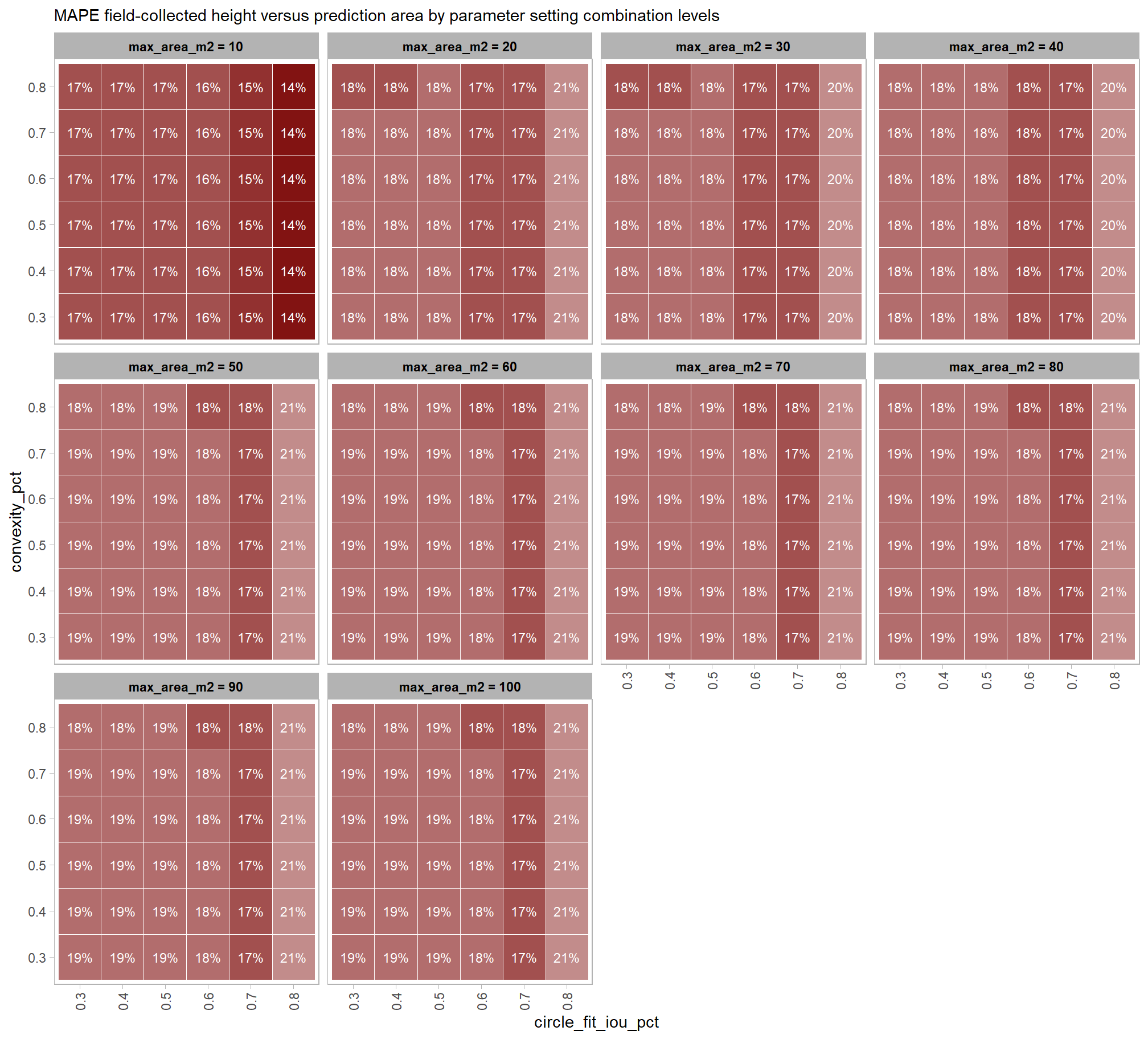
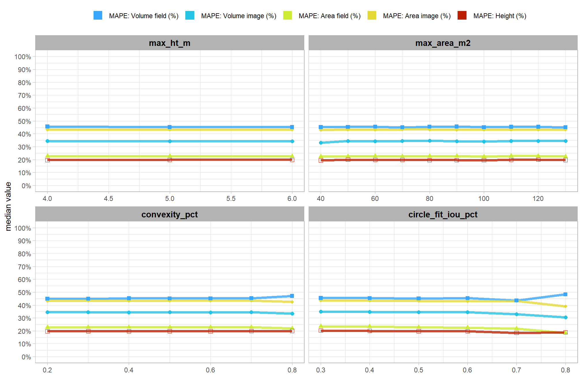
for this analysis, we’ll show how to calculate RRMSE but we’ll only investigate MAPE:
- Use MAPE when: You need an easily understandable metric for comparing prediction accuracy across different series or models with varying scales, particularly when zeros or near-zero actual values are not present in your data.
- Use RRMSE when: You need a metric that is more robust to small or zero actual values and you want to penalize larger errors more heavily due to the squaring of errors in its calculation.
as a reminder regarding the form quantification accuracy evaluation, we will assess the method’s accuracy by comparing the true-positive matches using the following metrics:
- Volume compares the predicted volume from the irregular elevation profile and footprint to the ground truth paraboloid volume
- Diameter compares the predicted diameter (from the maximum internal distance) to the ground truth field-measured diameter.
- Area compares the predicted area from the irregular shape to the ground truth assumed circular area
- Height compares the predicted maximum height from the CHM to the ground truth field-measured height
# first function takes df with cols tp_n, fp_n, and fn_n to calculate rate
confusion_matrix_scores_fn <- function(df) {
  df %>%
  dplyr::mutate(
    omission_rate = dplyr::case_when(
      (tp_n+fn_n) == 0  ~ as.numeric(NA)
      , T ~ fn_n/(tp_n+fn_n)
    ) # False Negative Rate or Miss Rate
    , commission_rate = dplyr::case_when(
      (tp_n+fp_n) == 0  ~ as.numeric(NA)
      , T ~ fp_n/(tp_n+fp_n)
    ) # False Positive Rate
    , precision = dplyr::case_when(
      (tp_n+fp_n) == 0  ~ as.numeric(NA)
      , T ~ tp_n/(tp_n+fp_n)
    )
    , recall = dplyr::case_when(
      (tp_n+fn_n) == 0  ~ as.numeric(NA)
      , T ~ tp_n/(tp_n+fn_n)
    )
    , f_score = dplyr::case_when(
      is.na(precision) | is.na(recall) ~ as.numeric(NA)
      , (precision+recall) == 0 ~ 0
      , T ~ 2 * ( (precision*recall)/(precision+recall) )
    )
  )
}
# aggregate results from ground_truth_prediction_match()
agg_ground_truth_match <- function(ground_truth_prediction_match_ans) {
  if(nrow(ground_truth_prediction_match_ans)==0){return(NULL)}
  if( !(names(ground_truth_prediction_match_ans) %>% stringr::str_equal("match_grp") %>% any()) ){stop("ground_truth_prediction_match_ans must contain `match_grp` column")}

  # check for difference columns (contains "_diff") and calc rmse for only those to return a single line df with colums for each diff_rmse
    if(
      (ground_truth_prediction_match_ans %>%
        dplyr::select(tidyselect::contains("_diff") & !tidyselect::starts_with("pct_")) %>%
        ncol() )>0
    ){
      # get rmse and mean difference/error for all columns with "_diff" but not "pct_diff"
      # get mape for all columns with "pct_diff" but not "diff_"
      rmse_df <- ground_truth_prediction_match_ans %>%
        dplyr::select(
          (tidyselect::contains("_diff") & !tidyselect::starts_with("pct_"))
          | tidyselect::starts_with("pct_diff")
        ) %>%
        tidyr::pivot_longer(dplyr::everything(), values_drop_na = T) %>%
        dplyr::group_by(name) %>%
        dplyr::summarise(
          sq = sum(value^2, na.rm = T)
          , mean = mean(value, na.rm = T)
          , sumabs = sum(abs(value), na.rm = T)
          , nomiss = sum(!is.na(value))
        ) %>%
        dplyr::ungroup() %>%
        dplyr::mutate(
          rmse = dplyr::case_when(
            dplyr::coalesce(nomiss,0)==0 ~ as.numeric(NA)
            , T ~ sqrt(sq/nomiss)
          )
          , mape = dplyr::case_when(
            dplyr::coalesce(nomiss,0)==0 ~ as.numeric(NA)
            , T ~ sumabs/nomiss
          )
        ) %>%
        # NA nonsense values
        dplyr::mutate(
          mape = dplyr::case_when(
            stringr::str_starts(name, "pct_diff") ~ mape
            , T ~ as.numeric(NA)
          )
          , rmse = dplyr::case_when(
            stringr::str_starts(name, "pct_diff") ~ as.numeric(NA)
            , T ~ rmse
          )
          , mean = dplyr::case_when(
            stringr::str_starts(name, "pct_diff") ~ as.numeric(NA)
            , T ~ mean
          )
        ) %>%
        dplyr::select(name,rmse,mean,mape) %>%
        tidyr::pivot_wider(
          names_from = name
          , values_from = c(rmse,mean,mape)
          , names_glue = "{name}_{.value}"
        ) %>%
        # remove columns with NA in all rows
        dplyr::select( dplyr::where( ~!all(is.na(.x)) ) )

      if(
        dplyr::coalesce(nrow(rmse_df),0)==0
        || dplyr::coalesce(ncol(rmse_df),0)==0
      ){
        # empty df
        rmse_df <- dplyr::tibble()
      }
    }else{
      # empty df
      rmse_df <- dplyr::tibble()
    }

  # count by match group
    agg <-
      ground_truth_prediction_match_ans %>%
      dplyr::count(match_grp) %>%
      dplyr::mutate(
        match_grp = dplyr::case_match(
          match_grp
          , "true positive"~"tp"
          , "commission"~"fp"
          , "omission"~"fn"
        )
      )
    # true positive, false positive, false negative rates
    return_df <- dplyr::tibble(match_grp = c("tp","fp","fn")) %>%
      dplyr::left_join(agg, by = "match_grp") %>%
      dplyr::mutate(dplyr::across(.cols = c(n), .fn = ~dplyr::coalesce(.x,0))) %>%
      tidyr::pivot_wider(
        names_from = match_grp
        , values_from = c(n)
        , names_glue = "{match_grp}_{.value}"
      )
    # rates, precision, recall, f-score
    return_df <- return_df %>%
      confusion_matrix_scores_fn() %>%
      # add rmse
      dplyr::bind_cols(rmse_df)
  # return
  return(return_df)
}
now let’s apply it at the parameter combination level
param_combos_gt_agg <- unique(param_combos_gt$rn) %>%
  purrr::map(\(x)
    agg_ground_truth_match(
      param_combos_gt %>%
        dplyr::filter(
          is_in_stand
          & rn == x
        )
    ) %>%
    dplyr::mutate(rn = x)
  ) %>%
  dplyr::bind_rows() %>%
  # add in info on all parameter combinations
  dplyr::inner_join(
    param_combos_piles %>%
    sf::st_drop_geometry() %>%
    dplyr::distinct(
      rn,max_ht_m,min_area_m2,max_area_m2,convexity_pct,circle_fit_iou_pct
    )
    , by = "rn"
    , relationship = "one-to-one"
  )

# we can also add the relative rmse (rrmse) by comparing the rmse to the mean value of the ground truth data
param_combos_gt_agg <- param_combos_gt_agg %>%
  dplyr::bind_cols(
    # add means of gt
    slash_piles_polys %>%
      sf::st_drop_geometry() %>%
      dplyr::select(image_gt_area_m2,field_gt_area_m2,image_gt_volume_m3,field_gt_volume_m3,height_m,field_diameter_m) %>%
      dplyr::ungroup() %>%
      dplyr::summarise(dplyr::across(dplyr::everything(), ~mean(.x,na.rm=T))) %>%
      dplyr::rename_with(~ paste0("gt_", .x, recycle0 = TRUE))
  ) %>%
  dplyr::mutate(
    area_diff_field_rrmse = area_diff_field_rmse/gt_field_gt_area_m2
    # , area_diff_image_rrmse = area_diff_image_rmse/gt_image_gt_area_m2
    , volume_diff_field_rrmse = volume_diff_field_rmse/gt_field_gt_volume_m3
    # , volume_diff_image_rrmse = volume_diff_image_rmse/gt_image_gt_volume_m3
    # , paraboloid_volume_diff_field_rrmse = paraboloid_volume_diff_field_rmse/gt_field_gt_volume_m3
    # , paraboloid_volume_diff_image_rrmse = paraboloid_volume_diff_image_rmse/gt_image_gt_volume_m3
    , height_diff_rrmse = height_diff_rmse/gt_height_m
    , diameter_diff_rrmse = diameter_diff_rmse/gt_field_diameter_m
  ) %>%
  dplyr::select(!tidyselect::starts_with("gt_"))
# what is this?
param_combos_gt_agg %>% dplyr::glimpse()
## Rows: 1,440
## Columns: 30
## $ tp_n <dbl> 79, 73, 65, 54, 32, 4, 79, 73, 65, 54, 32, …
## $ fp_n <dbl> 44, 32, 17, 9, 0, 0, 44, 32, 17, 9, 0, 0, 4…
## $ fn_n <dbl> 42, 48, 56, 67, 89, 117, 42, 48, 56, 67, 89…
## $ omission_rate <dbl> 0.3471074, 0.3966942, 0.4628099, 0.5537190,…
## $ commission_rate <dbl> 0.3577236, 0.3047619, 0.2073171, 0.1428571,…
## $ precision <dbl> 0.6422764, 0.6952381, 0.7926829, 0.8571429,…
## $ recall <dbl> 0.65289256, 0.60330579, 0.53719008, 0.44628…
## $ f_score <dbl> 0.6475410, 0.6460177, 0.6403941, 0.5869565,…
## $ area_diff_field_rmse <dbl> 1.611770, 1.664736, 1.626639, 1.638681, 1.6…
## $ diameter_diff_rmse <dbl> 0.7485177, 0.7525893, 0.7488925, 0.7384185,…
## $ height_diff_rmse <dbl> 0.3094341, 0.3178506, 0.3062417, 0.3100133,…
## $ volume_diff_field_rmse <dbl> 2.134892, 2.206145, 2.192266, 2.191718, 2.0…
## $ area_diff_field_mean <dbl> 0.022080324, 0.021422253, -0.002900846, -0.…
## $ diameter_diff_mean <dbl> 0.6528961, 0.6522134, 0.6509824, 0.6366149,…
## $ height_diff_mean <dbl> -0.2040260, -0.2230022, -0.2209795, -0.2303…
## $ volume_diff_field_mean <dbl> -0.8267348, -0.8985110, -0.8974220, -0.8900…
## $ pct_diff_area_field_mape <dbl> 0.1775634, 0.1861107, 0.1824384, 0.1827844,…
## $ pct_diff_diameter_mape <dbl> 0.2236866, 0.2242669, 0.2226649, 0.2205699,…
## $ pct_diff_height_mape <dbl> 0.1295703, 0.1335366, 0.1332140, 0.1357417,…
## $ pct_diff_volume_field_mape <dbl> 0.2357586, 0.2456211, 0.2479493, 0.2558522,…
## $ rn <dbl> 1, 2, 3, 4, 5, 6, 7, 8, 9, 10, 11, 12, 13, …
## $ max_ht_m <dbl> 2, 2, 2, 2, 2, 2, 2, 2, 2, 2, 2, 2, 2, 2, 2…
## $ min_area_m2 <dbl> 2, 2, 2, 2, 2, 2, 2, 2, 2, 2, 2, 2, 2, 2, 2…
## $ max_area_m2 <dbl> 10, 10, 10, 10, 10, 10, 10, 10, 10, 10, 10,…
## $ convexity_pct <dbl> 0.3, 0.3, 0.3, 0.3, 0.3, 0.3, 0.4, 0.4, 0.4…
## $ circle_fit_iou_pct <dbl> 0.3, 0.4, 0.5, 0.6, 0.7, 0.8, 0.3, 0.4, 0.5…
## $ area_diff_field_rrmse <dbl> 0.1519422, 0.1569353, 0.1533438, 0.1544791,…
## $ volume_diff_field_rrmse <dbl> 0.1396832, 0.1443452, 0.1434371, 0.1434012,…
## $ height_diff_rrmse <dbl> 0.1417985, 0.1456554, 0.1403356, 0.1420639,…
## $ diameter_diff_rrmse <dbl> 0.2162193, 0.2173954, 0.2163276, 0.2133020,…6.3 Parameter Sensitivity Test Results
let’s get a quick summary of the evaluation metrics across all parameter combinations
# pal
pal_eval_metric <- c(
  RColorBrewer::brewer.pal(3,"Oranges")[3]
  , RColorBrewer::brewer.pal(3,"Greys")[3]
  , RColorBrewer::brewer.pal(3,"Purples")[3]
)
# summary
param_combos_gt_agg %>%
  dplyr::select(f_score,recall,precision,tidyselect::ends_with("_mape")) %>%
  summary()
## f_score recall precision pct_diff_area_field_mape
## Min. :0.0640 Min. :0.03306 Min. :0.2905 Min. :0.1062
## 1st Qu.:0.5062 1st Qu.:0.48760 1st Qu.:0.5119 1st Qu.:0.2193
## Median :0.5986 Median :0.69421 Median :0.6456 Median :0.2270
## Mean :0.5474 Mean :0.60348 Mean :0.6569 Mean :0.2227
## 3rd Qu.:0.6900 3rd Qu.:0.84298 3rd Qu.:0.8020 3rd Qu.:0.2346
## Max. :0.7572 Max. :0.91736 Max. :1.0000 Max. :0.2569
## pct_diff_diameter_mape pct_diff_height_mape pct_diff_volume_field_mape
## Min. :0.1343 Min. :0.09824 Min. :0.1032
## 1st Qu.:0.2404 1st Qu.:0.14032 1st Qu.:0.2832
## Median :0.2493 Median :0.17690 Median :0.2962
## Mean :0.2440 Mean :0.16937 Mean :0.2919
## 3rd Qu.:0.2564 3rd Qu.:0.19214 3rd Qu.:0.3151
## Max. :0.3053 Max. :0.20849 Max. :0.34246.3.1 Overall: pile detection
let’s check out the distribution of the instance segmentation (i.e. pile detection) results by looking at the detection accuracy metrics where:
- Precision precision measures how many of the objects our method detected as slash piles were actually correct. A high precision means the method has a low rate of false alarms.
- Recall recall (i.e. detection rate) indicates how many actual (ground truth) slash piles our method successfully identified. High recall means the method is good at finding most existing piles, minimizing omissions.
- F-score provides a single, balanced measure that combines both precision and recall. A high F-score indicates overall effectiveness in both finding most piles and ensuring most detections are correct.
# this is a lot of work, so we're going to make it a function
plt_detection_dist <- function(
  df
  , my_subtitle = ""
  , show_rug = T
) {
  pal_eval_metric <- c(
    RColorBrewer::brewer.pal(3,"Oranges")[3]
    , RColorBrewer::brewer.pal(3,"Greys")[3]
    , RColorBrewer::brewer.pal(3,"Purples")[3]
  )

  df_temp <- df %>%
    tidyr::pivot_longer(
      cols = c(precision,recall,f_score)
      , names_to = "metric"
      , values_to = "value"
    ) %>%
    dplyr::mutate(
      metric = dplyr::case_when(
          metric == "f_score" ~ 1
          , metric == "recall" ~ 2
          , metric == "precision" ~ 3
        ) %>%
        factor(
          ordered = T
          , levels = 1:3
          , labels = c(
            "F-score"
            , "Recall"
            , "Precision"
          )
        )
    )

  # plot
  # if(nrow(df)<=15 && (df_temp %>% dplyr::count(metric,value) %>% dplyr::pull(n) %>% max())>1 ){
  if(nrow(df)<=15){
    # round
    df_temp <- df_temp %>%
      dplyr::mutate(
        value = round(value,2)
      )
    # agg for median plotting
      xxxdf_temp <- df_temp %>%
        dplyr::group_by(metric) %>%
        dplyr::summarise(value = median(value,na.rm=T)) %>%
        dplyr::ungroup() %>%
        dplyr::mutate(
          value_lab = paste0(
            "median:\n"
            , scales::percent(value,accuracy=1)
          )
        )

    # plot
    plt <- df_temp %>%
      dplyr::count(metric,value) %>%
      ggplot2::ggplot(
        mapping = ggplot2::aes(x = value, fill = metric, color = metric)
      ) +
      ggplot2::geom_vline(
        data = xxxdf_temp
        , mapping = ggplot2::aes(xintercept = value)
        , color = "gray44", linetype = "dashed"
      ) +
      # ggplot2::geom_jitter(mapping = ggplot2::aes(y=-0.2), width = 0, height = 0.1) +
      # ggplot2::geom_boxplot(width = 0.1, color = "black", fill = NA, outliers = F) +
      ggplot2::geom_segment(
        mapping = ggplot2::aes(y=n,yend=0)
        , lwd = 2, alpha = 0.8
      ) +
      ggplot2::geom_point(
        mapping = ggplot2::aes(y=n)
        , alpha = 1
        , shape = 21, color = "gray44", size = 5
      ) +
      ggplot2::geom_text(
        mapping = ggplot2::aes(y=n,label=n)
        , size = 2.5, color = "white"
        # , vjust = -0.01
      ) +
      ggplot2::geom_text(
        data = xxxdf_temp
        , mapping = ggplot2::aes(
          x = -Inf, y = Inf # always in upper left?
          # x = value, y = 0
          , label = value_lab
        )
        , hjust = -0.1, vjust = 1 # always in upper left?
        # , hjust = -0.1, vjust = -5
        , size = 2.5, color = "black"
      ) +
      # ggplot2::geom_rug() +
      ggplot2::scale_fill_manual(values = pal_eval_metric) +
      ggplot2::scale_color_manual(values = pal_eval_metric) +
      ggplot2::scale_x_continuous(
        labels = scales::percent_format(accuracy = 1)
        # , limits = c(0,1)
      ) +
      ggplot2::scale_y_continuous(expand = ggplot2::expansion(mult = c(0, .1))) +
      ggplot2::facet_grid(cols = dplyr::vars(metric), scales = "free") +
      ggplot2::labs(
        x = "", y = ""
        , subtitle = my_subtitle
      ) +
      ggplot2::theme_light() +
      ggplot2::theme(
        legend.position = "none"
        , strip.text = ggplot2::element_text(size = 11, color = "black", face = "bold")
        , axis.text.x = ggplot2::element_text(size = 7)
        , axis.text.y = ggplot2::element_blank()
        , axis.ticks.y = ggplot2::element_blank()
        , panel.grid.major.y = ggplot2::element_blank()
        , panel.grid.minor.y = ggplot2::element_blank()
        , plot.subtitle = ggplot2::element_text(size = 8)
      )
  }else{
    # agg for median plotting
      xxxdf_temp <- df_temp %>%
        dplyr::group_by(metric) %>%
        dplyr::summarise(value = median(value,na.rm=T)) %>%
        dplyr::ungroup() %>%
        dplyr::mutate(
          value_lab = paste0(
            "median:\n"
            , scales::percent(value,accuracy=1)
          )
        )

    plt <- df_temp %>%
      ggplot2::ggplot(
        mapping = ggplot2::aes(x = value, fill = metric, color = metric)
      ) +
      ggplot2::geom_density(color = NA, alpha = 0.8) +
      # ggplot2::geom_rug(
      #   # # setting these makes the plotting more computationally intensive
      #   # alpha = 0.5
      #   # , length = ggplot2::unit(0.01, "npc")
      # ) +
      ggplot2::geom_vline(
        data = xxxdf_temp
        , mapping = ggplot2::aes(xintercept = value)
        , color = "gray44", linetype = "dashed"
      ) +
      ggplot2::geom_text(
        data = xxxdf_temp
        , mapping = ggplot2::aes(
          x = -Inf, y = Inf # always in upper left?
          # x = value, y = 0
          , label = value_lab
        )
        , hjust = -0.1, vjust = 1 # always in upper left?
        # , hjust = -0.1, vjust = -5
        , size = 2.5, color = "black"
      ) +
      ggplot2::scale_fill_manual(values = pal_eval_metric) +
      ggplot2::scale_color_manual(values = pal_eval_metric) +
      ggplot2::scale_x_continuous(
        labels = scales::percent_format(accuracy = 1)
        # , limits = c(0,1)
      ) +
      ggplot2::facet_grid(cols = dplyr::vars(metric), scales = "free") +
      ggplot2::labs(
        x = "", y = ""
        , subtitle = my_subtitle
      ) +
      ggplot2::theme_light() +
      ggplot2::theme(
        legend.position = "none"
        , strip.text = ggplot2::element_text(size = 11, color = "black", face = "bold")
        , axis.text.x = ggplot2::element_text(size = 7)
        , axis.text.y = ggplot2::element_blank()
        , axis.ticks.y = ggplot2::element_blank()
        , panel.grid.major.y = ggplot2::element_blank()
        , panel.grid.minor.y = ggplot2::element_blank()
        , plot.subtitle = ggplot2::element_text(size = 8)
      )
    if(show_rug){
      plt <- plt +
        ggplot2::geom_rug(
          # # setting these makes the plotting more computationally intensive
          # alpha = 0.5
          # , length = ggplot2::unit(0.01, "npc")
        )
    }
  }
  return(plt)
}

# plot it
plt_detection_dist(
  df = param_combos_gt_agg
  , paste0(
     "distribution of pile detection accuracy metrics for all"
     , " (n="
     , scales::comma(nrow(param_combos_gt_agg), accuracy = 1)
     , ") "
     , "parameter combinations tested"
    )
)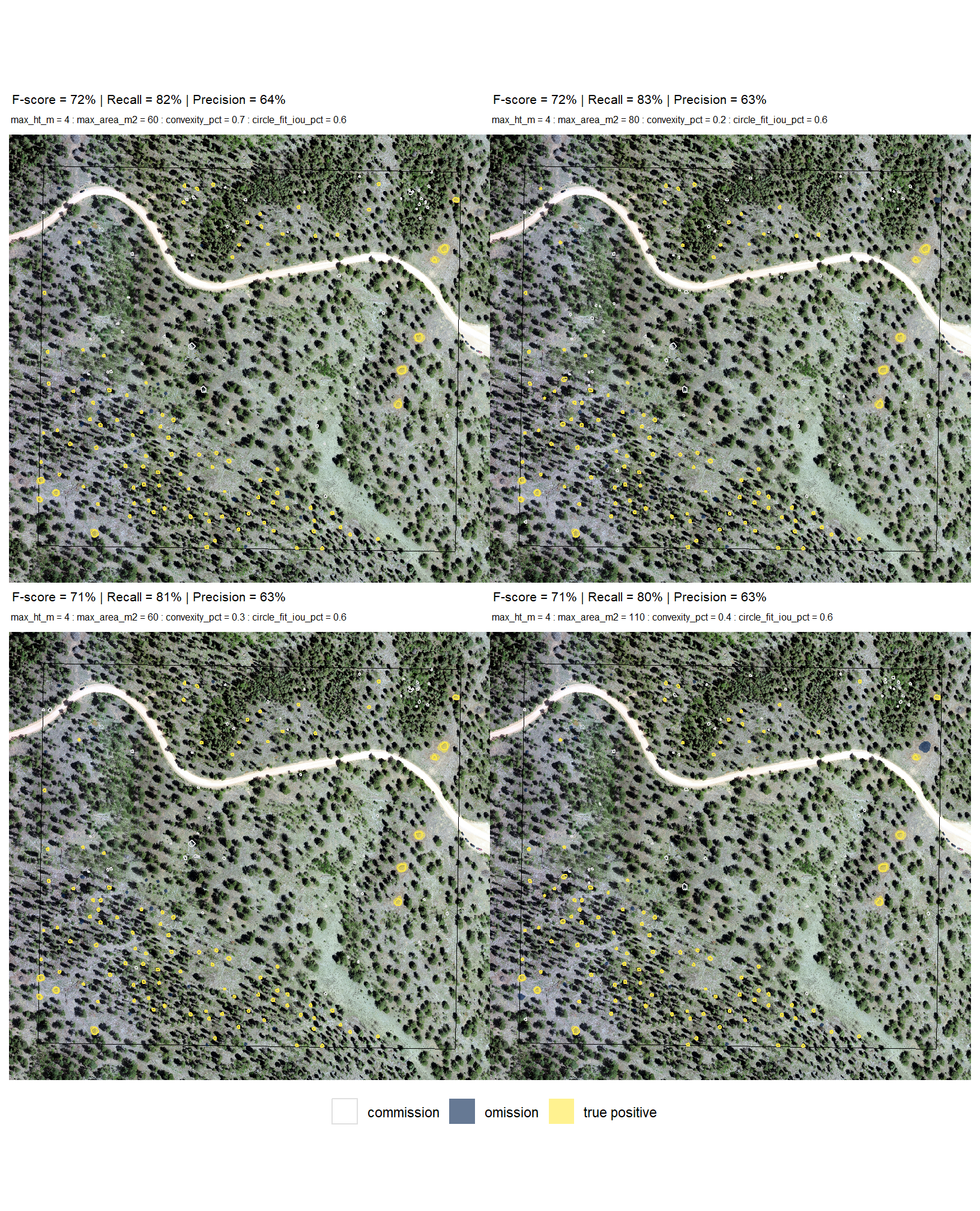
6.3.2 Overall: form quantification
let’s check out the the ability of the method to properly extract the form of the piles by looking at the quantification accuracy metrics where:
- Mean Error (ME) represents the direction of bias (over or under-prediction) in the original units
- RMSE represents the typical magnitude of error in the original units, with a stronger penalty for large errors
- MAPE represents the typical magnitude of error as a percentage, allowing for scale-independent comparisons
as a reminder regarding the form quantification accuracy evaluation, we will assess the method’s accuracy by comparing the true-positive matches using the following metrics:
- Volume compares the predicted volume from the irregular elevation profile and footprint to the ground truth paraboloid volume
- Diameter compares the predicted diameter (from the maximum internal distance) to the ground truth field-measured diameter.
- Area compares the predicted area from the irregular shape to the ground truth assumed circular area
- Height compares the predicted maximum height from the CHM to the ground truth field-measured height
# this is a lot of work, so we're going to make it a function
plt_form_quantification_dist <- function(
  df
  , my_subtitle = ""
  , show_rug = T
) {
  # reshape data to go long by evaluation metric
  df_temp <-
    df %>%
    dplyr::ungroup() %>%
    dplyr::mutate(
      # label combining params
      lab = stringr::str_c(max_ht_m,max_area_m2,convexity_pct,circle_fit_iou_pct, sep = ":") %>%
        forcats::fct_reorder(f_score) # %>% forcats::fct_rev()
    ) %>%
    dplyr::select(
      max_ht_m,max_area_m2,convexity_pct,circle_fit_iou_pct
      , lab
      # quantification
      , tidyselect::ends_with("_rmse")
      , tidyselect::ends_with("_rrmse")
      , tidyselect::ends_with("_mean")
      , tidyselect::ends_with("_mape")
    ) %>%
    tidyr::pivot_longer(
      cols = c(
        tidyselect::ends_with("_rmse")
        , tidyselect::ends_with("_rrmse")
        , tidyselect::ends_with("_mean")
        , tidyselect::ends_with("_mape")
      )
      , names_to = "metric"
      , values_to = "value"
    ) %>%
    dplyr::mutate(
      eval_metric = stringr::str_extract(metric, "(_rmse|_rrmse|_mean|_mape)$") %>%
        stringr::str_remove_all("_") %>%
        stringr::str_replace_all("mean","me") %>%
        toupper() %>%
        factor(
          ordered = T
          , levels = c("ME","RMSE","RRMSE","MAPE")
        )
      , pile_metric = metric %>%
        stringr::str_remove("(_rmse|_rrmse|_mean|_mape)$") %>%
        stringr::str_extract("(paraboloid_volume|volume|area|height|diameter)") %>%
        factor(
          ordered = T
          , levels = c(
            "volume"
            , "paraboloid_volume"
            , "area"
            , "height"
            , "diameter"
          )
          , labels = c(
            "Volume"
            , "Volume paraboloid"
            , "Area"
            , "Height"
            , "Diameter"
          )
        )
    )

  # plot
  # !!! we map over the ggplot function to allow for differnt formatting of the x axis
  # !!! and to allow for different axis ranges for each individual panel which is not possible when faceting
  plt_list_temp <-
    # get factors in order
    df_temp %>%
    dplyr::filter(eval_metric!="RRMSE") %>%
    dplyr::count(eval_metric) %>%
    pull(eval_metric) %>%
    purrr::map(function(x, my_show_rug=show_rug){
      if(nrow(df)<=15){
        df_temp <- df_temp %>%
          dplyr::filter(eval_metric==x) %>%
          dplyr::mutate(
            value = dplyr::case_when(
              eval_metric %in% c("RRMSE", "MAPE") ~ round(value,2)
              , T ~ round(value,1)
            )
          )
        # aggregate
        xxxdf_temp <- df_temp %>%
          dplyr::group_by(pile_metric,eval_metric) %>%
          dplyr::summarise(value = median(value,na.rm=T)) %>%
          dplyr::ungroup() %>%
          dplyr::mutate(
            value_lab = paste0(
                "median:\n"
              , dplyr::case_when(
                eval_metric %in% c("RRMSE", "MAPE") ~ scales::percent(value,accuracy=1)
                , eval_metric == "ME" ~ scales::comma(value,accuracy=0.1)
                , T ~ scales::comma(value,accuracy=0.1)
              )
            )
          )
        # plot
        p <- df_temp %>%
          dplyr::count(eval_metric,pile_metric,value) %>%
          ggplot2::ggplot(
            mapping = ggplot2::aes(x = value, fill = pile_metric, color = pile_metric)
          ) +
          ggplot2::geom_vline(
            data = xxxdf_temp
            , mapping = ggplot2::aes(xintercept = value)
            , color = "gray44", linetype = "dashed"
          ) +
          # ggplot2::geom_jitter(mapping = ggplot2::aes(y=-0.2), width = 0, height = 0.1) +
          # ggplot2::geom_boxplot(width = 0.1, color = "black", fill = NA, outliers = F) +
          ggplot2::geom_segment(
            mapping = ggplot2::aes(y=n,yend=0)
            , lwd = 2, alpha = 0.8
          ) +
          ggplot2::geom_point(
            mapping = ggplot2::aes(y=n)
            , alpha = 1
            , shape = 21, color = "gray44", size = 5
          ) +
          ggplot2::geom_text(
            mapping = ggplot2::aes(y=n,label=n)
            , size = 2.5, color = "white"
            # , vjust = -0.01
          ) +
          ggplot2::geom_text(
            data = xxxdf_temp
            , mapping = ggplot2::aes(
              x = -Inf, y = Inf # always in upper left?
              # x = value, y = 0
              , label = value_lab
            )
            , hjust = -0.1, vjust = 1 # always in upper left?
            # , hjust = -0.1, vjust = -5
            , size = 2.5, color = "black"
          ) +
          # ggplot2::geom_rug() +
          ggplot2::scale_fill_viridis_d(option = "turbo") +
          ggplot2::scale_color_viridis_d(option = "turbo") +
          ggplot2::scale_y_continuous(expand = ggplot2::expansion(mult = c(0, .33))) +
          ggplot2::facet_grid(
            cols = dplyr::vars(pile_metric), rows = dplyr::vars(eval_metric)
            , scales = "free"
            , switch = "y" # moves y facet label to left
          ) +
          ggplot2::labs(x = "", y = "") +
          ggplot2::theme_light() +
          ggplot2::theme(
            legend.position = "none"
            , strip.placement = "outside"
            , strip.text.y = ggplot2::element_text(size = 11, color = "black", face = "bold")
            , strip.text.y.left = ggplot2::element_text(angle = 0)
            , strip.background.y = ggplot2::element_rect(color = NA, fill = NA)
            , strip.text.x = ggplot2::element_text(size = 8, color = "black", face = "bold")
            , axis.text.x = ggplot2::element_text(size = 6.5)
            , axis.text.y = ggplot2::element_blank()
            , axis.ticks.y = ggplot2::element_blank()
            , panel.grid.major.y = ggplot2::element_blank()
            , panel.grid.minor.y = ggplot2::element_blank()
          )
      }else{
        # aggregate
        xxxdf_temp <- df_temp %>%
          dplyr::group_by(pile_metric,eval_metric) %>%
          dplyr::summarise(value = median(value,na.rm=T)) %>%
          dplyr::ungroup() %>%
          dplyr::mutate(
            value_lab = paste0(
                "median:\n"
              , dplyr::case_when(
                eval_metric %in% c("RRMSE", "MAPE") ~ scales::percent(value,accuracy=1)
                , eval_metric == "ME" ~ scales::comma(value,accuracy=0.1)
                , T ~ scales::comma(value,accuracy=0.1)
              )
            )
          )
        p <- df_temp %>%
          dplyr::filter(eval_metric==x) %>%
          ggplot2::ggplot() +
          # ggplot2::geom_vline(xintercept = 0, color = "gray") +
          ggplot2::geom_density(mapping = ggplot2::aes(x = value, fill = pile_metric), color = NA, alpha = 0.8) +
          # ggplot2::geom_rug(mapping = ggplot2::aes(x = value, color = pile_metric)) +
          ggplot2::scale_fill_viridis_d(option = "turbo") +
          ggplot2::scale_color_viridis_d(option = "turbo") +
          ggplot2::geom_vline(
            data = xxxdf_temp %>% dplyr::filter(eval_metric==x)
            , mapping = ggplot2::aes(xintercept = value)
            , color = "gray44", linetype = "dashed"
          ) +
          ggplot2::geom_text(
            data = xxxdf_temp %>% dplyr::filter(eval_metric==x)
            , mapping = ggplot2::aes(
              x = -Inf, y = Inf # always in upper left?
              # x = value, y = 0
              , label = value_lab
            )
            , hjust = -0.1, vjust = 1 # always in upper left?
            # , hjust = -0.1, vjust = -5
            , size = 2.5
          ) +
          ggplot2::facet_grid(
            cols = dplyr::vars(pile_metric), rows = dplyr::vars(eval_metric)
            , scales = "free"
            , switch = "y" # moves y facet label to left
          ) +
          ggplot2::labs(x = "", y = "") +
          ggplot2::theme_light() +
          ggplot2::theme(
            legend.position = "none"
            , strip.placement = "outside"
            , strip.text.y = ggplot2::element_text(size = 11, color = "black", face = "bold")
            , strip.text.y.left = ggplot2::element_text(angle = 0)
            , strip.background.y = ggplot2::element_rect(color = NA, fill = NA)
            , strip.text.x = ggplot2::element_text(size = 8, color = "black", face = "bold")
            , axis.text.x = ggplot2::element_text(size = 6.5)
            , axis.text.y = ggplot2::element_blank()
            , axis.ticks.y = ggplot2::element_blank()
            , panel.grid.major.y = ggplot2::element_blank()
            , panel.grid.minor.y = ggplot2::element_blank()
          )

        if(my_show_rug){
          p <- p + ggplot2::geom_rug(mapping = ggplot2::aes(x = value, color = pile_metric))
        }
      }

      if(x %in% c("RRMSE", "MAPE")){
        return(p+ggplot2::scale_x_continuous(labels = scales::percent_format(accuracy = 1)))
      }else{
        return(p)
      }
    })
  # combine
  # plt_list_temp
  patchwork::wrap_plots(
      plt_list_temp
      , ncol = 1
  ) + patchwork::plot_annotation(
      # title = paste0(aoi_sf$study_site_lab, " - ALS")
      subtitle = my_subtitle
        # paste0(
        #      "distribution of pile form quantification accuracy metrics for all"
        #      # , scales::percent(1-pct_rank_th_top,accuracy=1)
        #      , " (n="
        #      , scales::comma(nrow(param_combos_gt_agg), accuracy = 1)
        #      , ") "
        #      , "parameter combinations tested"
        #   )
      # , caption = "hey"
      , theme = ggplot2::theme(
        plot.subtitle = ggplot2::element_text(size = 8)
      )
    )
}
# plot it
plt_form_quantification_dist(
  df = param_combos_gt_agg
  , paste0(
     "distribution of pile form quantification accuracy metrics for all"
     , " (n="
     , scales::comma(nrow(param_combos_gt_agg), accuracy = 1)
     , ") "
     , "parameter combinations tested"
  )
)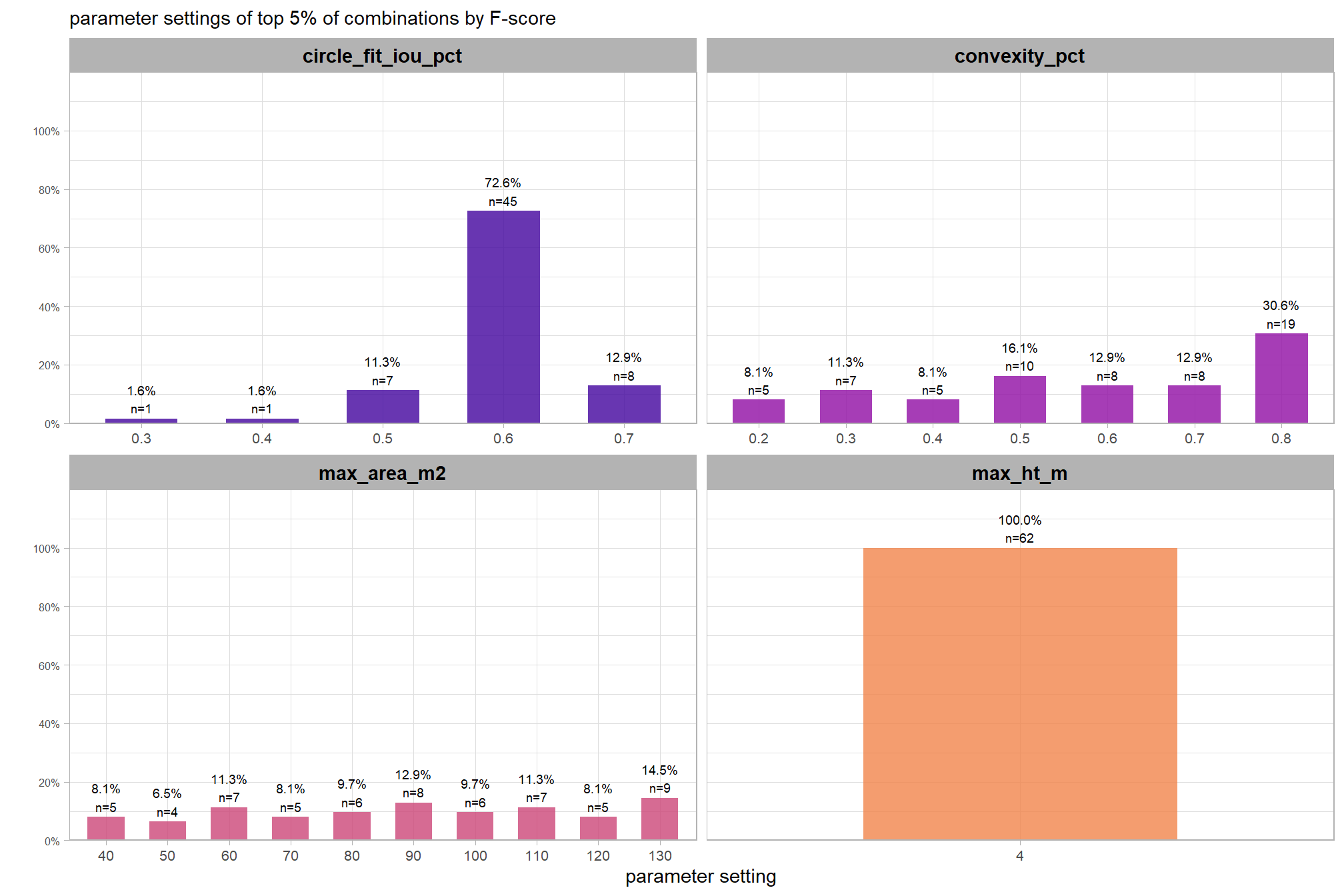
6.3.3 Main Effects: pile detection
let’s average across all other factors to look at the main effect by parameter for instance segmentation performance (i.e. pile detection)
param_combos_gt_agg %>%
  tidyr::pivot_longer(
    cols = c(precision,recall,f_score)
    , names_to = "metric"
    , values_to = "value"
  ) %>%
  tidyr::pivot_longer(
    cols = c(max_ht_m,max_area_m2,convexity_pct,circle_fit_iou_pct)
    , names_to = "param"
    , values_to = "param_value"
  ) %>%
  dplyr::group_by(param, param_value, metric) %>%
  dplyr::summarise(
    median = median(value,na.rm=T)
    , q25 = stats::quantile(value,na.rm=T,probs = 0.25)
    , q75 = stats::quantile(value,na.rm=T,probs = 0.75)
  ) %>%
  dplyr::ungroup() %>%
  dplyr::mutate(
    param = dplyr::case_when(
        param == "max_ht_m" ~ 1
        , param == "min_area_m2" ~ 2
        , param == "max_area_m2" ~ 3
        , param == "convexity_pct" ~ 4
        , param == "circle_fit_iou_pct" ~ 5
      ) %>%
      factor(
        ordered = T
        , levels = 1:5
        , labels = c(
          "max_ht_m"
          , "min_area_m2"
          , "max_area_m2"
          , "convexity_pct"
          , "circle_fit_iou_pct"
        )
      )
    , metric = dplyr::case_when(
        metric == "f_score" ~ 1
        , metric == "recall" ~ 2
        , metric == "precision" ~ 3
      ) %>%
      factor(
        ordered = T
        , levels = 1:3
        , labels = c(
          "F-score"
          , "Recall"
          , "Precision"
        )
      )
  ) %>%
  ggplot2::ggplot(
    mapping = ggplot2::aes(y = median, x = param_value, color = metric, fill = metric, group = metric, shape = metric)
  ) +
  ggplot2::geom_ribbon(
    mapping = ggplot2::aes(ymin = q25, ymax = q75)
    , alpha = 0.2, color = NA
  ) +
  ggplot2::geom_line(lwd = 1.5, alpha = 0.8) +
  ggplot2::geom_point(size = 2) +
  ggplot2::facet_wrap(facets = dplyr::vars(param), scales = "free_x") +
  # ggplot2::scale_color_viridis_d(begin = 0.2, end = 0.8) +
  ggplot2::scale_fill_manual(values = pal_eval_metric) +
  ggplot2::scale_color_manual(values = pal_eval_metric) +
  ggplot2::scale_y_continuous(limits = c(0,1), labels = scales::percent, breaks = scales::breaks_extended(10)) +
  ggplot2::labs(x = "", y = "median value", color = "", fill = "") +
  ggplot2::theme_light() +
  ggplot2::theme(
    legend.position = "top"
    , strip.text = ggplot2::element_text(size = 11, color = "black", face = "bold")
  ) +
  ggplot2::guides(
    color = ggplot2::guide_legend(override.aes = list(shape = 15, linetype = 0, size = 5, alpha = 1))
    , shape = "none"
  )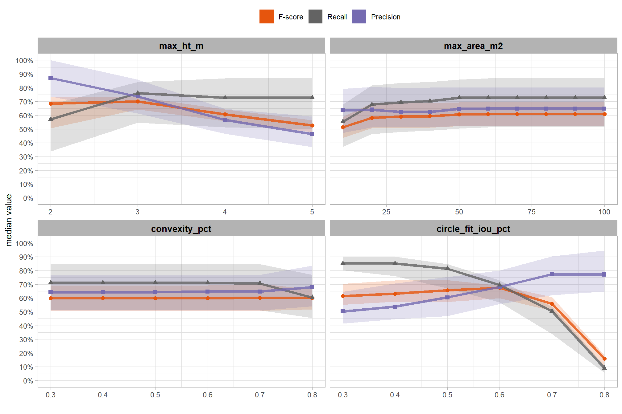
based on these main effect aggregated results:
- increasing the
max_ht_m(determines the “slice” of the CHM to use) reduces precision and F-score with minimal impact on recall - increasing the
max_area_m2(determines the maximum pile area) has minimal impact on all three evaluation metrics - increasing
convexity_pcttoward 1 to favor regular shapes had minimal impact on metrics until parameter values exceeded 0.7, at which point recall decreased, but precision and F-score slightly improved - increasing
circle_fit_iou_pcttoward 1 to favor circular shapes minimally affected recall while improving precision and F-score up to parameter values of 0.5. Beyond this, recall significantly dropped, with only modest F-score improvements, and overall accuracy measured by F-score crashed past 0.7
6.3.4 Main Effects: form quantification
let’s average across all other factors to look at the main effect by parameter for the MAPE metrics quantifying the pile form accuracy
param_combos_gt_agg %>%
  tidyr::pivot_longer(
    cols = c(tidyselect::ends_with("_mape"))
    , names_to = "metric"
    , values_to = "value"
  ) %>%
  tidyr::pivot_longer(
    cols = c(max_ht_m,max_area_m2,convexity_pct,circle_fit_iou_pct)
    , names_to = "param"
    , values_to = "param_value"
  ) %>%
  dplyr::group_by(param, param_value, metric) %>%
  dplyr::summarise(
    median = median(value,na.rm=T)
    , q25 = stats::quantile(value,na.rm=T,probs = 0.25)
    , q75 = stats::quantile(value,na.rm=T,probs = 0.75)
  ) %>%
  dplyr::ungroup() %>%
  dplyr::mutate(
    param = dplyr::case_when(
        param == "max_ht_m" ~ 1
        , param == "min_area_m2" ~ 2
        , param == "max_area_m2" ~ 3
        , param == "convexity_pct" ~ 4
        , param == "circle_fit_iou_pct" ~ 5
      ) %>%
      factor(
        ordered = T
        , levels = 1:5
        , labels = c(
          "max_ht_m"
          , "min_area_m2"
          , "max_area_m2"
          , "convexity_pct"
          , "circle_fit_iou_pct"
        )
      )
    , metric = dplyr::case_when(
        metric == "f_score" ~ 1
        , metric == "recall" ~ 2
        , metric == "precision" ~ 3
        # rmse
        , metric == "pct_diff_volume_field_mape" ~ 4
        , metric == "pct_diff_paraboloid_volume_field_mape" ~ 5
        , metric == "pct_diff_area_field_mape" ~ 6
        , metric == "pct_diff_height_mape" ~ 7
        , metric == "pct_diff_diameter_mape" ~ 8
      ) %>%
      factor(
        ordered = T
        , levels = 1:8
        , labels = c(
          "F-score"
          , "Recall"
          , "Precision"
          , "MAPE: Volume irregular (%)"
          , "MAPE: Volume paraboloid (%)"
          , "MAPE: Area (%)"
          , "MAPE: Height (%)"
          , "MAPE: Diameter (%)"
        )
      )
  ) %>%
  ggplot2::ggplot(
    mapping = ggplot2::aes(y = median, x = param_value, color = metric, fill = metric, group = metric, shape = metric)
  ) +
  # ggplot2::geom_ribbon(
  #   mapping = ggplot2::aes(ymin = q25, ymax = q75)
  #   , alpha = 0.2, color = NA
  # ) +
  ggplot2::geom_line(lwd = 1.5, alpha = 0.8) +
  ggplot2::geom_point(size = 2) +
  ggplot2::facet_wrap(facets = dplyr::vars(param), scales = "free_x") +
  ggplot2::scale_fill_viridis_d(option = "turbo") +
  ggplot2::scale_color_viridis_d(option = "turbo") +
  # ggplot2::scale_fill_manual(values = pal_get_pairs_fn(6)[1:5]) +
  # ggplot2::scale_color_manual(values = pal_get_pairs_fn(6)[1:5]) +
  ggplot2::scale_shape_manual(values = c(15,16,17,18,0)) +
  ggplot2::scale_y_continuous(limits = c(0,1), labels = scales::percent, breaks = scales::breaks_extended(10)) +
  ggplot2::labs(x = "", y = "median value", color = "", fill = "") +
  ggplot2::theme_light() +
  ggplot2::theme(
    legend.position = "top"
    , strip.text = ggplot2::element_text(size = 11, color = "black", face = "bold")
  ) +
  ggplot2::guides(
    color = ggplot2::guide_legend(override.aes = list(shape = 15, linetype = 0, size = 5, alpha = 1))
    , shape = "none"
  )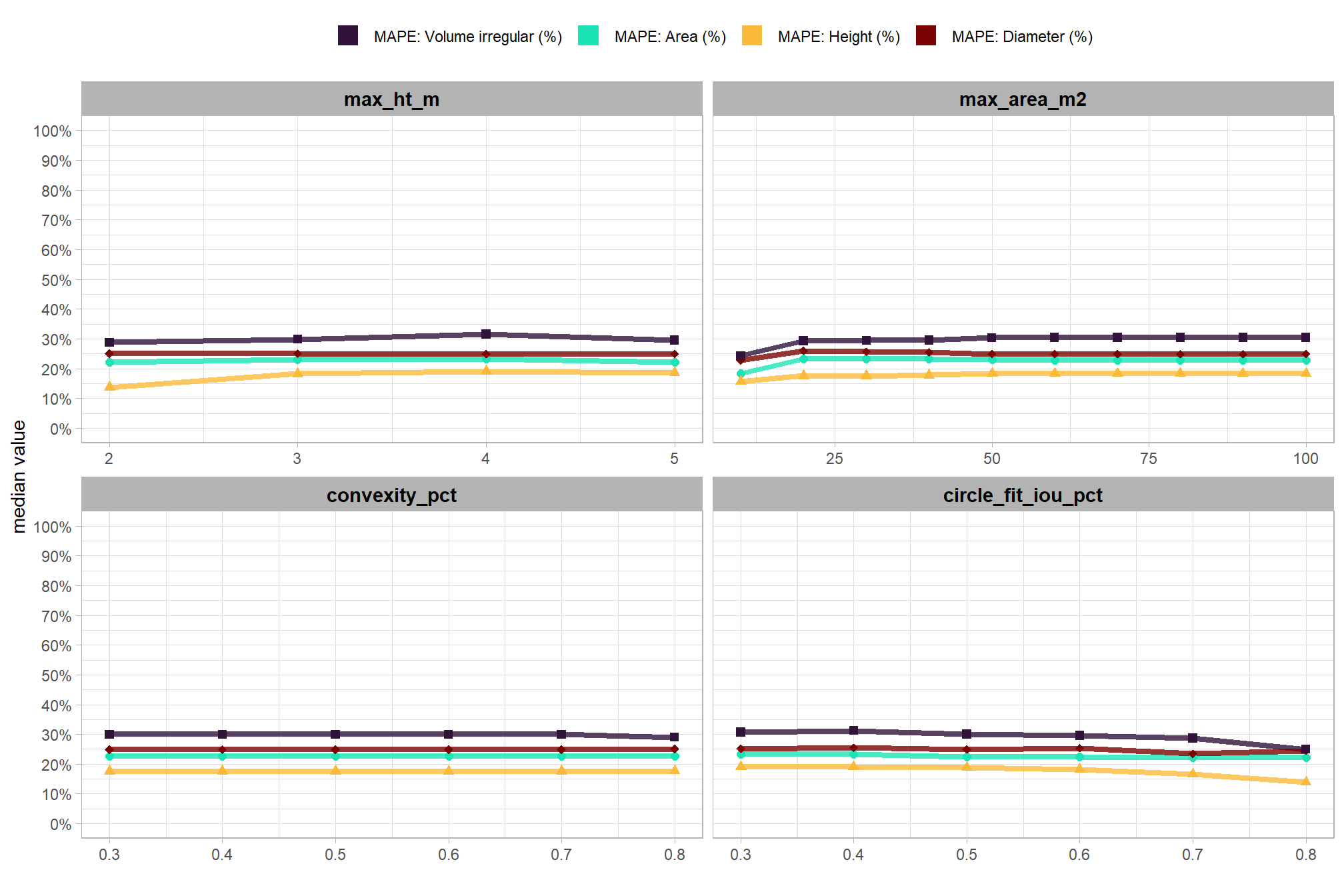
these results indicate that the method’s accuracy in outlining slash pile form is robust to parameter changes, as the relevant shape accuracy metrics remain consistent across various settings
6.3.5 Best results: detection accuracy
we can cut to the chase and just look at the parameter combinations that achieved the best results based on the detection accuracy metrics
pct_rank_th_temp <- 0.95
df_temp <-
  param_combos_gt_agg %>%
  dplyr::ungroup() %>%
  dplyr::arrange(desc(f_score), desc(recall), desc(precision), pct_diff_volume_field_mape) %>%
  dplyr::mutate(
    # label combining params
    lab = stringr::str_c(max_ht_m,max_area_m2,convexity_pct,circle_fit_iou_pct, sep = ":")
    , dplyr::across(
      .cols = c(f_score,precision,recall)
      , .fn = dplyr::percent_rank
      , .names = "pct_rank_{.col}"
    )
    , sort_lab = dplyr::row_number()
  ) %>%
  # dplyr::select(precision, pct_rank_precision) %>%
  # dplyr::arrange(desc(precision), desc(pct_rank_precision)) %>%
  # View()
  # now get the max of these pct ranks by row
  dplyr::rowwise() %>%
  dplyr::mutate(
    pct_rank_max = max(
      dplyr::c_across(
        tidyselect::starts_with("pct_rank")
      )
      , na.rm = T
    )
  ) %>%
  dplyr::ungroup() %>%
  dplyr::filter(pct_rank_max>=pct_rank_th_temp) %>%
  dplyr::select(
    rn,max_ht_m,max_area_m2,convexity_pct,circle_fit_iou_pct
    , lab, sort_lab
    , tidyselect::starts_with("pct_rank")
    , c(f_score,precision,recall)
    , -c(pct_rank_max)
  ) %>%
  # expand data to unique lab, pct_rank
  tidyr::pivot_longer(
    cols = tidyselect::starts_with("pct_rank")
    , names_to = "metric"
    , values_to = "value"
  ) %>%
  # keep only relevant records
  dplyr::filter(value>=pct_rank_th_temp) %>%
  dplyr::group_by(metric) %>%
  dplyr::arrange(desc(value),desc(f_score), desc(recall), desc(precision)) %>%
  dplyr::filter(dplyr::row_number()<=11) %>%
  dplyr::ungroup() %>%
  dplyr::mutate(
    rank_lab = stringr::str_remove(metric,"pct_rank_") %>%
      factor(
        ordered = T
        , levels = c(
          "f_score"
          , "recall"
          , "precision"
        )
        , labels = c(
          paste0("top ", scales::percent(1-pct_rank_th_temp, accuracy = 1), " F-Score") %>% stringr::str_wrap(width = 14)
          , paste0("top ", scales::percent(1-pct_rank_th_temp, accuracy = 1), " Recall") %>% stringr::str_wrap(width = 14)
          , paste0("top ", scales::percent(1-pct_rank_th_temp, accuracy = 1), " Precision") %>% stringr::str_wrap(width = 14)
        )
      )
  ) %>%
  dplyr::select(-c(metric,value))

# df_temp %>% dplyr::count(rank_lab)
# df_temp %>% dplyr::glimpse()

# plot
df_temp %>%
  tidyr::pivot_longer(
    cols = c(precision,recall,f_score)
    , names_to = "metric"
    , values_to = "value"
  ) %>%
  dplyr::mutate(
    metric = dplyr::case_when(
        metric == "f_score" ~ 1
        , metric == "recall" ~ 2
        , metric == "precision" ~ 3
      ) %>%
      factor(
        ordered = T
        , levels = 1:3
        , labels = c(
          "F-score"
          , "Recall"
          , "Precision"
        )
      )
    , lab = forcats::fct_reorder(lab, sort_lab) %>% forcats::fct_rev()
    , val_lab = scales::percent(value, accuracy = 0.1)
  ) %>%
  ggplot2::ggplot(
    mapping = ggplot2::aes(x = value, y = lab, fill = metric, label = val_lab)
  ) +
  ggplot2::geom_col(width = 0.6) +
  ggplot2::geom_text(color = "black", size = 2, hjust = -0.2) +
  ggplot2::scale_fill_manual(values = pal_eval_metric) +
  ggplot2::scale_x_continuous(
    labels = scales::percent_format(accuracy = 1)
    , limits = c(0,1.11)
    # , expand = expansion(mult = c(0, .08))
  ) +
  ggplot2::facet_grid(cols = dplyr::vars(metric), rows = dplyr::vars(rank_lab), scales = "free_y") +
  ggplot2::labs(
    x = "", y = "max_ht_m : max_area_m2 : convexity_pct : circle_fit_iou_pct"
    , fill = ""
    , subtitle = "top parameter combinations by evaluation metrics"
  ) +
  ggplot2::theme_light() +
  ggplot2::theme(
    legend.position = "none"
    , strip.text = ggplot2::element_text(size = 11, color = "black", face = "bold")
    , axis.text = ggplot2::element_text(size = 6)
  )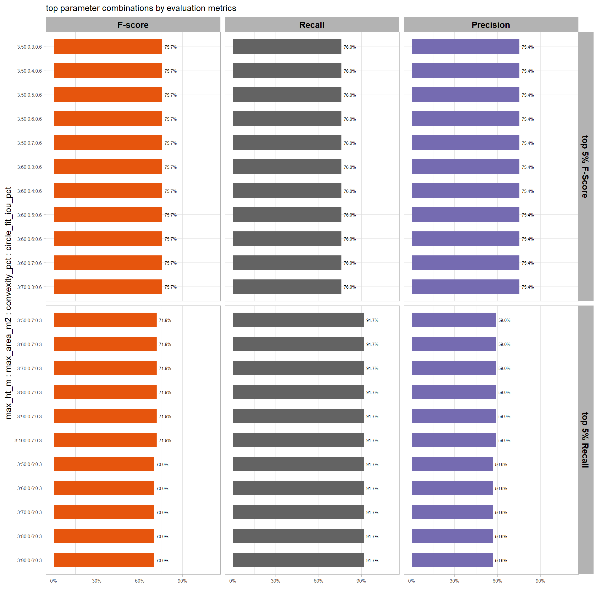
let’s make a table of these results
df_temp %>%
  dplyr::select(
    rank_lab
    , max_ht_m,max_area_m2,convexity_pct,circle_fit_iou_pct
    , f_score, recall, precision
  ) %>%
  dplyr::ungroup() %>%
  dplyr::arrange(rank_lab,desc(f_score), desc(recall), desc(precision)) %>%
  dplyr::mutate(dplyr::across(
    .cols = c(f_score, recall, precision)
    , .fn = ~ scales::percent(.x, accuracy = 1)
  )) %>%
  dplyr::mutate(blank= "   " ) %>%
  dplyr::relocate(blank, .before = f_score) %>%
  kableExtra::kbl(
    caption = "parameter combinations that achieved the best slash pile detection results"
    , col.names = c(
      "."
      ,"max_ht_m","max_area_m2","convexity_pct","circle_fit_iou_pct"
      , "   "
      , "F-score", "Recall", "Precision"
    )
    , escape = F
  ) %>%
  kableExtra::kable_styling(font_size = 11) %>%
  kableExtra::collapse_rows(columns = 1, valign = "top") %>%
kableExtra::add_header_above(c(" "=6, "Evaluation Metric" = 3))| . | max_ht_m | max_area_m2 | convexity_pct | circle_fit_iou_pct | F-score | Recall | Precision | |
|---|---|---|---|---|---|---|---|---|
| top 5% F-Score | 3 | 50 | 0.3 | 0.6 | 76% | 76% | 75% | |
| 3 | 50 | 0.4 | 0.6 | 76% | 76% | 75% | ||
| 3 | 50 | 0.5 | 0.6 | 76% | 76% | 75% | ||
| 3 | 50 | 0.6 | 0.6 | 76% | 76% | 75% | ||
| 3 | 50 | 0.7 | 0.6 | 76% | 76% | 75% | ||
| 3 | 60 | 0.3 | 0.6 | 76% | 76% | 75% | ||
| 3 | 60 | 0.4 | 0.6 | 76% | 76% | 75% | ||
| 3 | 60 | 0.5 | 0.6 | 76% | 76% | 75% | ||
| 3 | 60 | 0.6 | 0.6 | 76% | 76% | 75% | ||
| 3 | 60 | 0.7 | 0.6 | 76% | 76% | 75% | ||
| 3 | 70 | 0.3 | 0.6 | 76% | 76% | 75% | ||
| top 5% Recall | 3 | 50 | 0.7 | 0.3 | 72% | 92% | 59% | |
| 3 | 60 | 0.7 | 0.3 | 72% | 92% | 59% | ||
| 3 | 70 | 0.7 | 0.3 | 72% | 92% | 59% | ||
| 3 | 80 | 0.7 | 0.3 | 72% | 92% | 59% | ||
| 3 | 90 | 0.7 | 0.3 | 72% | 92% | 59% | ||
| 3 | 100 | 0.7 | 0.3 | 72% | 92% | 59% | ||
| 3 | 50 | 0.6 | 0.3 | 70% | 92% | 57% | ||
| 3 | 60 | 0.6 | 0.3 | 70% | 92% | 57% | ||
| 3 | 70 | 0.6 | 0.3 | 70% | 92% | 57% | ||
| 3 | 80 | 0.6 | 0.3 | 70% | 92% | 57% | ||
| 3 | 90 | 0.6 | 0.3 | 70% | 92% | 57% |
let’s check out maps of the pile detection results for the parameter combinations with the highest F-score
df_temp <-
  df_temp %>%
  dplyr::ungroup() %>%
  dplyr::arrange(desc(f_score), desc(recall), desc(precision)) %>%
  dplyr::select(
    rn, rank_lab
    , max_ht_m,max_area_m2,convexity_pct,circle_fit_iou_pct
    , f_score, recall, precision
  ) %>%
  dplyr::distinct() %>%
  dplyr::slice_head(n=4)
# ortho
ortho_plt_temp <- ortho_plt_fn(
    stand = sf::st_bbox(stand_boundary) %>%
      sf::st_as_sfc() %>%
      sf::st_transform(sf::st_crs(param_combos_piles))
    , buffer = 10
  )
# plot it
plt_list_temp <- 1:nrow(df_temp) %>%
  purrr::map(\(x)
    ortho_plt_temp +
    # ggplot2::ggplot() +
      ggplot2::geom_sf(
        data = stand_boundary %>%
          sf::st_transform(sf::st_crs(param_combos_piles))
        , color = "black", fill = NA
      ) +
      ggplot2::geom_sf(
        data =
          slash_piles_polys %>%
          dplyr::filter(is_in_stand) %>%
          sf::st_transform(sf::st_crs(param_combos_piles)) %>%
          dplyr::mutate(pile_id=as.numeric(pile_id)) %>%
            dplyr::left_join(
              param_combos_gt %>%
                dplyr::filter(rn == df_temp$rn[x]) %>%
                dplyr::select(pile_id,match_grp)
              , by = "pile_id"
            )
        , mapping = ggplot2::aes(fill = match_grp)
        , color = NA ,alpha=0.6
      ) +
      ggplot2::geom_sf(
        data =
          param_combos_piles %>%
            dplyr::filter(rn == df_temp$rn[x] & is_in_stand) %>%
            dplyr::left_join(
              param_combos_gt %>%
                dplyr::filter(rn == df_temp$rn[x] & is_in_stand) %>%
                dplyr::select(pred_id,match_grp)
              , by = "pred_id"
            )
        , mapping = ggplot2::aes(fill = match_grp, color = match_grp)
        , alpha = 0
        , lwd = 0.5
      ) +
      ggplot2::scale_fill_manual(values = pal_match_grp, name = "", na.value = "red") +
      ggplot2::scale_color_manual(values = pal_match_grp, name = "", na.value = "red") +
      ggplot2::labs(
        title = paste0(
          " F-score = ", scales::percent(df_temp$f_score[x], accuracy = 1)
          ," | Recall = ", scales::percent(df_temp$recall[x], accuracy = 1)
          ," | Precision = ", scales::percent(df_temp$precision[x], accuracy = 1)
        )
        , subtitle = paste0(
          " max_ht_m = ", (df_temp$max_ht_m[x])
          ," : max_area_m2 = ", (df_temp$max_area_m2[x])
          ," : convexity_pct = ", (df_temp$convexity_pct[x])
          ," : circle_fit_iou_pct = ", (df_temp$circle_fit_iou_pct[x])
          , "\n"
        )
      ) +
      ggplot2::theme_void() +
      ggplot2::theme(
        legend.position = "top"
        # , panel.background = ggplot2::element_rect(fill = "gray66")
        , plot.title = ggplot2::element_text(size = 8)
        , plot.subtitle = ggplot2::element_text(size = 6)
      ) +
      ggplot2::guides(
        fill = ggplot2::guide_legend(override.aes = list(color = c(pal_match_grp["commission"],NA,NA)))
        , color = "none"
      )
)patchwork::wrap_plots(
plt_list_temp
, ncol = 2
, guides = "collect"
) &
ggplot2::theme(legend.position = "bottom")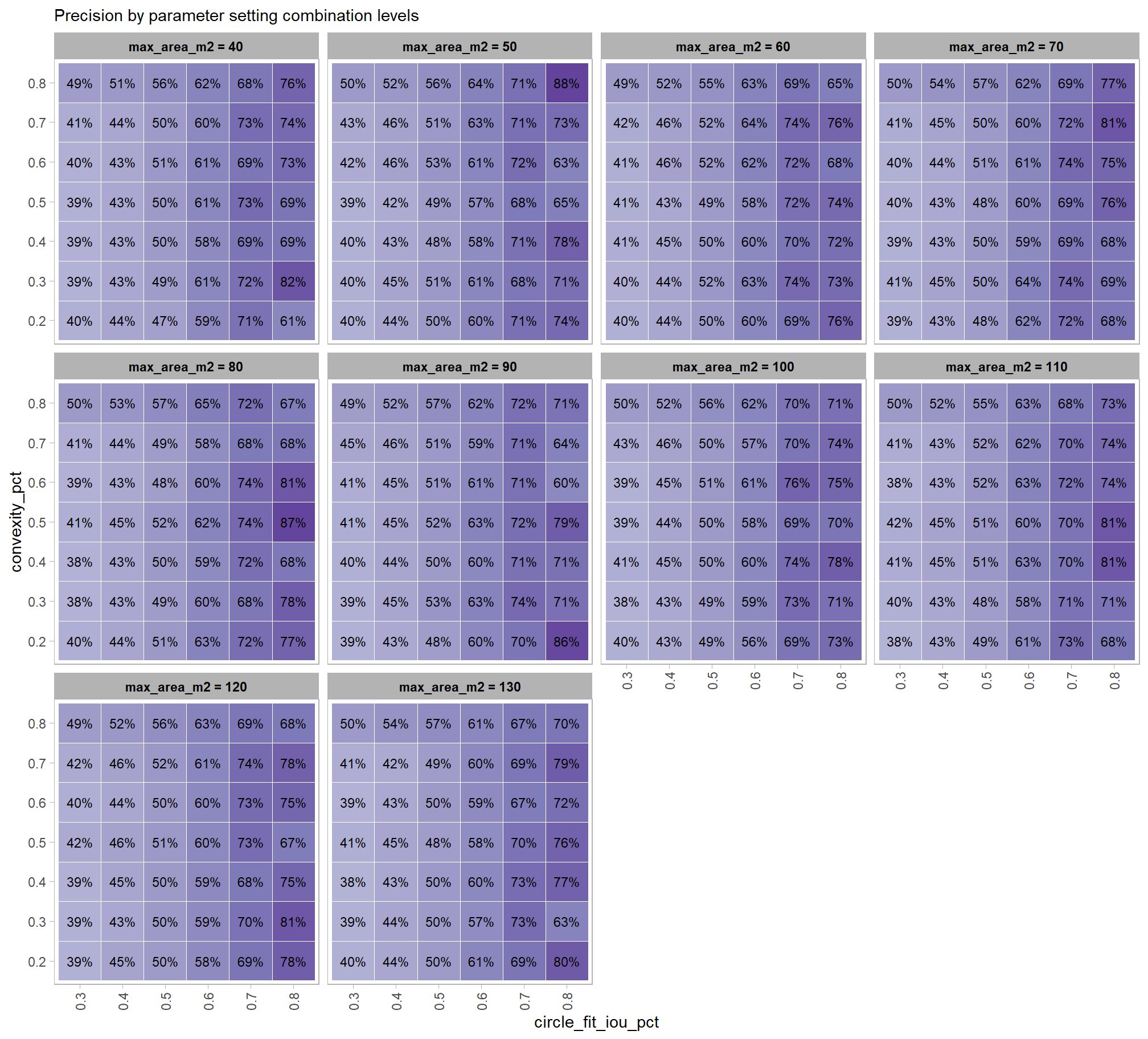
it looks like even for these best performing pile detection parameter combinations, there were false positive (commission) detections in areas with trees. These incorrect detections appear to be mostly in aspen groves where the short, clumped low trees resemble slash piles structurally. The integration of the spectral data should help to filter out these false positive predictions
let’s look at only the top 5% of parameter combinations by F-score
# filter parameter combos for top x pct
top_x_pct_fscore <-
  param_combos_gt_agg %>%
    dplyr::ungroup() %>%
    dplyr::arrange(desc(f_score)) %>%
    dplyr::mutate(
      pct_rank_f_score = dplyr::percent_rank(f_score)
    ) %>%
    dplyr::filter(pct_rank_f_score>=pct_rank_th_top)
# plot it
plt_detection_dist(
  df = top_x_pct_fscore
  , paste0(
     "distribution of evaluation metrics for top "
     , scales::percent(1-pct_rank_th_top,accuracy=1)
     , " (n="
     , scales::comma(nrow(top_x_pct_fscore), accuracy = 1)
     , ") "
     , "of parameter combinations by F-score using structural data only"
  )
)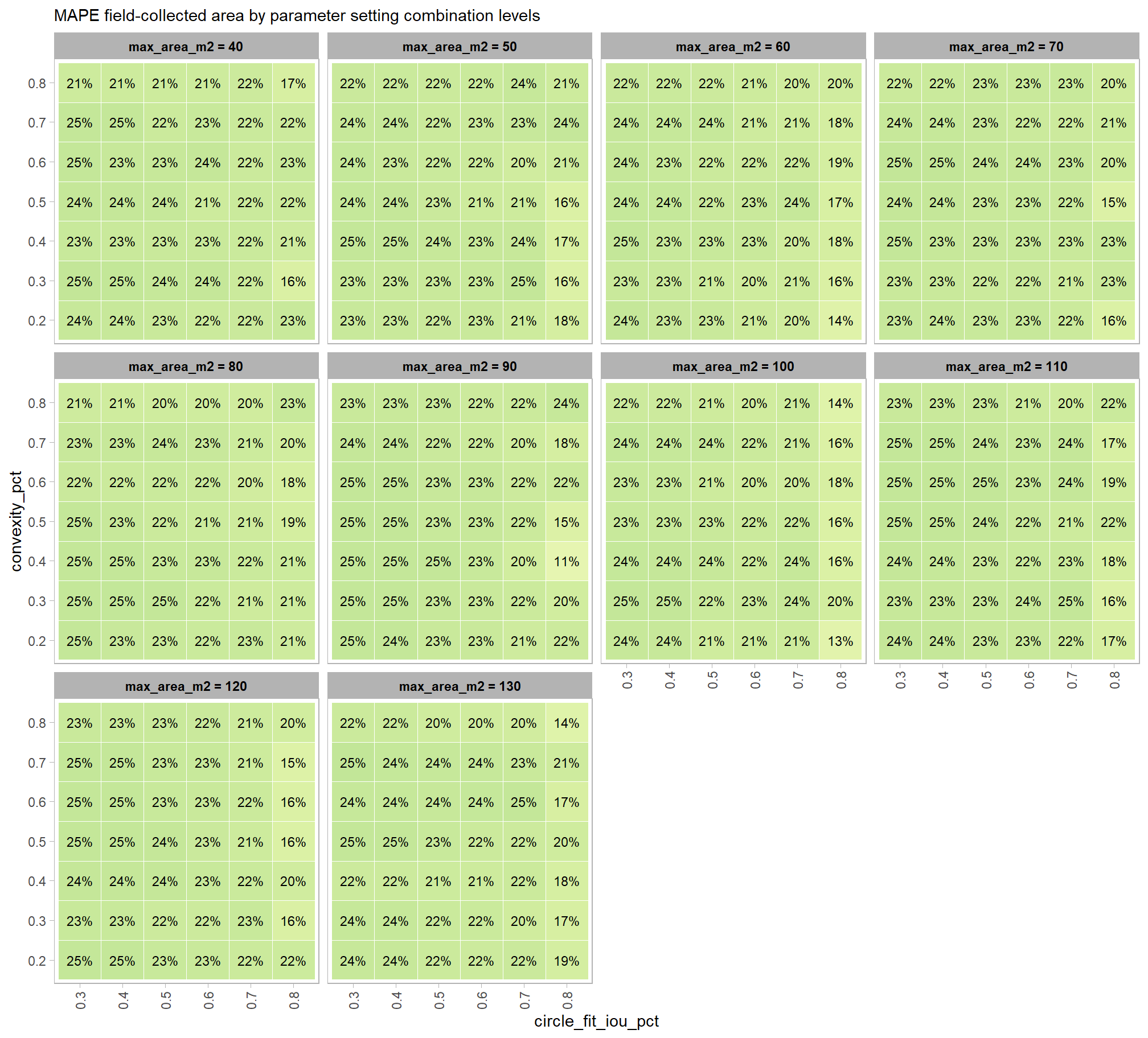
if we look at only the top 5% of parameter combinations by F-score, what is the distribution of individual parameter settings?
pal_param <- viridis::plasma(n=5, begin = 0.1, end = 0.9, alpha = 0.8)
top_x_pct_fscore %>%
  dplyr::select(tidyselect::contains("f_score"), max_ht_m,max_area_m2,convexity_pct,circle_fit_iou_pct) %>%
  tidyr::pivot_longer(
    cols = c(max_ht_m,max_area_m2,convexity_pct,circle_fit_iou_pct)
    , names_to = "metric"
    , values_to = "value"
  ) %>%
  dplyr::count(metric, value) %>%
  dplyr::group_by(metric) %>%
  dplyr::mutate(
    pct=n/sum(n)
    , lab = paste0(scales::percent(pct,accuracy=0.1), "\nn=", scales::comma(n,accuracy=1))
  ) %>%
  ggplot2::ggplot(
    mapping = ggplot2::aes(x = factor(value), y=pct, label=lab, fill = metric)
  ) +
  ggplot2::geom_col(width = 0.6) +
  ggplot2::geom_text(color = "black", size = 2.5, vjust = -0.2) +
  ggplot2::facet_wrap(facets = dplyr::vars(metric), ncol=2, scales = "free_x") +
  ggplot2::scale_y_continuous(
    breaks = seq(0,1,by=0.2)
    , labels = scales::percent
    , expand = ggplot2::expansion(mult = c(0,0.2))
  ) +
  ggplot2::scale_fill_manual(values = pal_param[1:4]) +
  ggplot2::labs(
    x = "parameter setting", y = ""
    , fill = ""
    , subtitle = paste0(
       "parameter settings of top "
       , scales::percent(1-pct_rank_th_top,accuracy=1)
       , " (n="
       , scales::comma(nrow(top_x_pct_fscore), accuracy = 1)
       , ") "
       , "of parameter combinations by F-score using structural data only"
    )
  ) +
  ggplot2::theme_light() +
  ggplot2::theme(
    legend.position = "none"
    , strip.text = ggplot2::element_text(size = 11, color = "black", face = "bold")
    , axis.text.y = ggplot2::element_text(size = 6)
    , axis.text.x = ggplot2::element_text(size = 8)
    , plot.subtitle = ggplot2::element_text(size = 8)
  )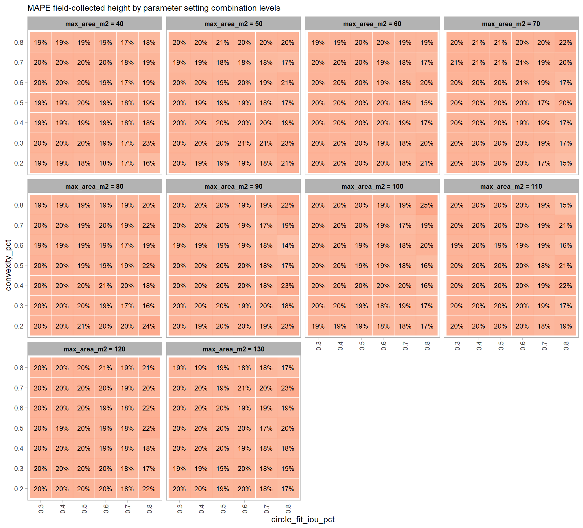
6.3.6 Best results: quantification accuracy
we can cut to the chase and just look at the parameter combinations that achieved the best results based on the form quantification accuracy metrics
pct_rank_th_temp <- 0.99
df_temp <-
  param_combos_gt_agg %>%
  dplyr::arrange(pct_diff_volume_field_mape, pct_diff_diameter_mape, pct_diff_area_field_mape, pct_diff_height_mape) %>%
  dplyr::mutate(
    # label combining params
    lab = stringr::str_c(max_ht_m,max_area_m2,convexity_pct,circle_fit_iou_pct, sep = ":")
    , dplyr::across(
      .cols = c(tidyselect::ends_with("_mape"))
      , .fn = dplyr::percent_rank
      , .names = "pct_rank_{.col}"
    )
  ) %>%
  # dplyr::arrange(pct_diff_diameter_mape) %>%
  # dplyr::select(pct_diff_diameter_mape, pct_rank_pct_diff_diameter_mape) %>%
  # now get the max of these pct ranks by row
  dplyr::rowwise() %>%
  dplyr::mutate(
    pct_rank_min = min(
      dplyr::c_across(
        tidyselect::starts_with("pct_rank")
      )
      , na.rm = T
    )
  ) %>%
  dplyr::ungroup() %>%
  dplyr::filter(pct_rank_min<=(1-pct_rank_th_temp)) %>%
  dplyr::select(
    max_ht_m,max_area_m2,convexity_pct,circle_fit_iou_pct
    , lab
    , tidyselect::starts_with("pct_rank")
    , tidyselect::starts_with("pct_diff")
    , -c(pct_rank_min)
  ) %>%
  # get sort for lab
  dplyr::group_by(lab) %>%
  dplyr::mutate(sort_lab = pct_rank_pct_diff_volume_field_mape) %>%
  dplyr::ungroup() %>%
  # expand data to unique lab, pct_rank
  tidyr::pivot_longer(
    cols = tidyselect::starts_with("pct_rank")
    , names_to = "metric"
    , values_to = "value"
  ) %>%
  # keep only relevant records
  dplyr::filter(value<=(1-pct_rank_th_temp)) %>%
  dplyr::group_by(metric) %>%
  dplyr::arrange(pct_diff_volume_field_mape, pct_diff_diameter_mape, pct_diff_area_field_mape, pct_diff_height_mape) %>%
  dplyr::filter(dplyr::row_number()<=11) %>%
  dplyr::ungroup() %>%
  dplyr::mutate(
    rank_lab = stringr::str_remove(metric,"pct_rank_") %>%
      factor(
        ordered = T
        , levels = c(
          "pct_diff_volume_field_mape"
          , "pct_diff_paraboloid_volume_field_mape"
          , "pct_diff_area_field_mape"
          , "pct_diff_height_mape"
          , "pct_diff_diameter_mape"
        )
        , labels = c(
          paste0("top ", scales::percent(1-pct_rank_th_temp, accuracy = 1), " MAPE Volume irregular") %>% stringr::str_wrap(width = 14)
          , paste0("top ", scales::percent(1-pct_rank_th_temp, accuracy = 1), " MAPE Volume paraboloid") %>% stringr::str_wrap(width = 14)
          , paste0("top ", scales::percent(1-pct_rank_th_temp, accuracy = 1), " MAPE Area") %>% stringr::str_wrap(width = 14)
          , paste0("top ", scales::percent(1-pct_rank_th_temp, accuracy = 1), " MAPE Height") %>% stringr::str_wrap(width = 14)
          , paste0("top ", scales::percent(1-pct_rank_th_temp, accuracy = 1), " MAPE Diameter") %>% stringr::str_wrap(width = 14)
        )
      )
  ) %>%
  dplyr::select(-c(metric,value))

  # dplyr::group_by(lab) %>%
  # dplyr::mutate(xxx = dplyr::n()) %>%
  # dplyr::ungroup() %>%
  # dplyr::arrange(desc(xxx), lab) %>%
  # View()
# df_temp %>% dplyr::glimpse()

df_temp %>%
  tidyr::pivot_longer(
    cols = tidyselect::starts_with("pct_diff_")
    , names_to = "metric"
    , values_to = "value"
  ) %>%
  dplyr::mutate(
    metric = dplyr::case_when(
        metric == "pct_diff_volume_field_mape" ~ 1
        , metric == "pct_diff_paraboloid_volume_field_mape" ~ 2
        , metric == "pct_diff_area_field_mape" ~ 3
        , metric == "pct_diff_height_mape" ~ 4
        , metric == "pct_diff_diameter_mape" ~ 5
      ) %>%
      factor(
        ordered = T
        , levels = 1:5
        , labels = c(
          "MAPE Volume irregular"
          , "MAPE Volume paraboloid"
          , "MAPE Area"
          , "MAPE Height"
          , "MAPE Diameter"
        )
      )
    , lab = forcats::fct_reorder(lab, sort_lab) %>% forcats::fct_rev()
    , val_lab = scales::percent(value, accuracy = 0.1)
  ) %>%
  ggplot2::ggplot(
    mapping = ggplot2::aes(x = value, y = lab, fill = metric, label = val_lab)
  ) +
  ggplot2::geom_col(width = 0.6) +
  ggplot2::geom_text(color = "black", size = 2, hjust = -0.2) +
  ggplot2::scale_fill_viridis_d(option = "turbo") +
  # ggplot2::scale_fill_manual(values = pal_get_pairs_fn(6)[1:5][c(1,3,5)]) +
  ggplot2::scale_x_continuous(
    labels = scales::percent_format(accuracy = 1)
    , limits = c(0,1.05)
    # , expand = expansion(mult = c(0, .08))
  ) +
  ggplot2::facet_grid(cols = dplyr::vars(metric), rows = dplyr::vars(rank_lab), scales = "free_y") +
  ggplot2::labs(
    x = "", y = "max_ht_m : max_area_m2 : convexity_pct : circle_fit_iou_pct"
    , fill = ""
    , subtitle = paste0(
       "pile shape quantification accuracy for top "
       , scales::percent(1-pct_rank_th_temp,accuracy=1)
       , " of parameter combinations"
    )
  ) +
  ggplot2::theme_light() +
  ggplot2::theme(
    legend.position = "none"
    , strip.text = ggplot2::element_text(size = 11, color = "black", face = "bold")
    , axis.text = ggplot2::element_text(size = 6)
  )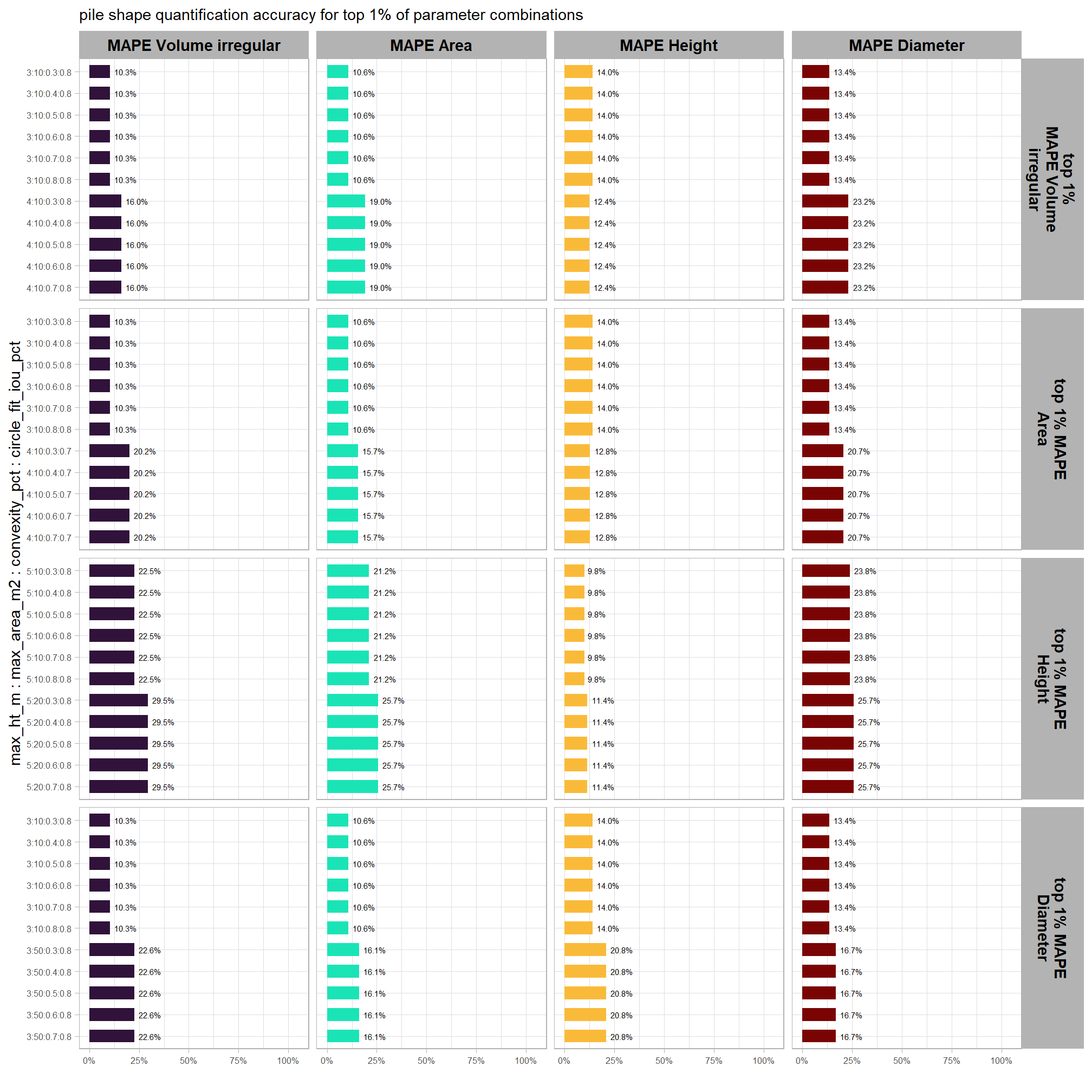
let’s make a table of these results
df_temp %>%
  dplyr::select(
    rank_lab
    , max_ht_m,max_area_m2,convexity_pct,circle_fit_iou_pct
    , pct_diff_volume_field_mape, pct_diff_area_field_mape, pct_diff_height_mape, pct_diff_diameter_mape
  ) %>%
  dplyr::ungroup() %>%
  dplyr::arrange(rank_lab,pct_diff_volume_field_mape, pct_diff_area_field_mape, pct_diff_height_mape, pct_diff_diameter_mape) %>%
  dplyr::mutate(dplyr::across(
    .cols = tidyselect::starts_with("pct_diff_")
    , .fn = ~ scales::percent(.x, accuracy = 1)
  )) %>%
  dplyr::mutate(blank= "   " ) %>%
  dplyr::relocate(blank, .before = pct_diff_volume_field_mape) %>%
  kableExtra::kbl(
    caption = "parameter combinations that achieved the best slash pile form quantification results"
    , col.names = c(
      "."
      ,"max_ht_m","max_area_m2","convexity_pct","circle_fit_iou_pct"
      , "   "
      , "MAPE Volume irregular"
      , "MAPE Area"
      , "MAPE Height"
      , "MAPE Diameter"
    )
    , escape = F
  ) %>%
  kableExtra::kable_styling(font_size = 11) %>%
  kableExtra::collapse_rows(columns = 1, valign = "top") %>%
kableExtra::add_header_above(c(" "=6, "Evaluation Metric" = 4))| . | max_ht_m | max_area_m2 | convexity_pct | circle_fit_iou_pct | MAPE Volume irregular | MAPE Area | MAPE Height | MAPE Diameter | |
|---|---|---|---|---|---|---|---|---|---|
| top 1% MAPE Volume irregular | 3 | 10 | 0.3 | 0.8 | 10% | 11% | 14% | 13% | |
| 3 | 10 | 0.4 | 0.8 | 10% | 11% | 14% | 13% | ||
| 3 | 10 | 0.5 | 0.8 | 10% | 11% | 14% | 13% | ||
| 3 | 10 | 0.6 | 0.8 | 10% | 11% | 14% | 13% | ||
| 3 | 10 | 0.7 | 0.8 | 10% | 11% | 14% | 13% | ||
| 3 | 10 | 0.8 | 0.8 | 10% | 11% | 14% | 13% | ||
| 4 | 10 | 0.3 | 0.8 | 16% | 19% | 12% | 23% | ||
| 4 | 10 | 0.4 | 0.8 | 16% | 19% | 12% | 23% | ||
| 4 | 10 | 0.5 | 0.8 | 16% | 19% | 12% | 23% | ||
| 4 | 10 | 0.6 | 0.8 | 16% | 19% | 12% | 23% | ||
| 4 | 10 | 0.7 | 0.8 | 16% | 19% | 12% | 23% | ||
| top 1% MAPE Area | 3 | 10 | 0.3 | 0.8 | 10% | 11% | 14% | 13% | |
| 3 | 10 | 0.4 | 0.8 | 10% | 11% | 14% | 13% | ||
| 3 | 10 | 0.5 | 0.8 | 10% | 11% | 14% | 13% | ||
| 3 | 10 | 0.6 | 0.8 | 10% | 11% | 14% | 13% | ||
| 3 | 10 | 0.7 | 0.8 | 10% | 11% | 14% | 13% | ||
| 3 | 10 | 0.8 | 0.8 | 10% | 11% | 14% | 13% | ||
| 4 | 10 | 0.3 | 0.7 | 20% | 16% | 13% | 21% | ||
| 4 | 10 | 0.4 | 0.7 | 20% | 16% | 13% | 21% | ||
| 4 | 10 | 0.5 | 0.7 | 20% | 16% | 13% | 21% | ||
| 4 | 10 | 0.6 | 0.7 | 20% | 16% | 13% | 21% | ||
| 4 | 10 | 0.7 | 0.7 | 20% | 16% | 13% | 21% | ||
| top 1% MAPE Height | 5 | 10 | 0.3 | 0.8 | 23% | 21% | 10% | 24% | |
| 5 | 10 | 0.4 | 0.8 | 23% | 21% | 10% | 24% | ||
| 5 | 10 | 0.5 | 0.8 | 23% | 21% | 10% | 24% | ||
| 5 | 10 | 0.6 | 0.8 | 23% | 21% | 10% | 24% | ||
| 5 | 10 | 0.7 | 0.8 | 23% | 21% | 10% | 24% | ||
| 5 | 10 | 0.8 | 0.8 | 23% | 21% | 10% | 24% | ||
| 5 | 20 | 0.3 | 0.8 | 29% | 26% | 11% | 26% | ||
| 5 | 20 | 0.4 | 0.8 | 29% | 26% | 11% | 26% | ||
| 5 | 20 | 0.5 | 0.8 | 29% | 26% | 11% | 26% | ||
| 5 | 20 | 0.6 | 0.8 | 29% | 26% | 11% | 26% | ||
| 5 | 20 | 0.7 | 0.8 | 29% | 26% | 11% | 26% | ||
| top 1% MAPE Diameter | 3 | 10 | 0.3 | 0.8 | 10% | 11% | 14% | 13% | |
| 3 | 10 | 0.4 | 0.8 | 10% | 11% | 14% | 13% | ||
| 3 | 10 | 0.5 | 0.8 | 10% | 11% | 14% | 13% | ||
| 3 | 10 | 0.6 | 0.8 | 10% | 11% | 14% | 13% | ||
| 3 | 10 | 0.7 | 0.8 | 10% | 11% | 14% | 13% | ||
| 3 | 10 | 0.8 | 0.8 | 10% | 11% | 14% | 13% | ||
| 3 | 50 | 0.3 | 0.8 | 23% | 16% | 21% | 17% | ||
| 3 | 50 | 0.4 | 0.8 | 23% | 16% | 21% | 17% | ||
| 3 | 50 | 0.5 | 0.8 | 23% | 16% | 21% | 17% | ||
| 3 | 50 | 0.6 | 0.8 | 23% | 16% | 21% | 17% | ||
| 3 | 50 | 0.7 | 0.8 | 23% | 16% | 21% | 17% |
if we look at only the top 5% of parameter combinations by F-score, which quantifies the method’s ability to accurately detect slash piles, what is the distribution of the pile form quantification accuracy metrics?
# plot it
plt_form_quantification_dist(
  df = top_x_pct_fscore
  , paste0(
     "distribution of pile form quantification metrics for the top "
     , scales::percent(1-pct_rank_th_top,accuracy=1)
     , " (n="
     , scales::comma(nrow(top_x_pct_fscore), accuracy = 1)
     , ") "
     , "of parameter combinations by F-score using structural data only"
  )
)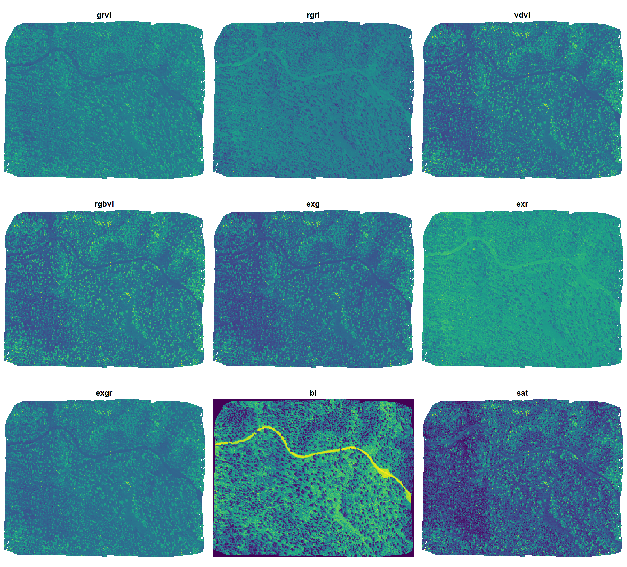
these don’t look much better than the overall form quantification accuracy metrics based on all parameter combinations tested
6.3.7 Best results: detection & quantification
as we saw immediately above, the form quantification accuracy metrics for the top 5% of parameter combinations by F-score don’t appear to be much better than the quantification accuracy metrics using all parameter combinations tested. let’s check to see if there is a relationship between the quantification and detection accuracy metrics using data from all parameter combinations tested
param_combos_gt_agg %>%
  dplyr::ungroup() %>%
  dplyr::select(
    rn,max_ht_m,max_area_m2,convexity_pct,circle_fit_iou_pct
    , f_score
    # quantification accuracy
    , tidyselect::ends_with("_mape")
  ) %>%
  tidyr::pivot_longer(
    cols = c(tidyselect::ends_with("_mape"))
    , names_to = "metric"
    , values_to = "value"
  ) %>%
  dplyr::mutate(
    eval_metric = stringr::str_extract(metric, "(_rmse|_rrmse|_mean|_mape)$") %>%
      stringr::str_remove_all("_") %>%
      stringr::str_replace_all("mean","me") %>%
      toupper() %>%
      factor(
        ordered = T
        , levels = c("ME","RMSE","RRMSE","MAPE")
      )
    , pile_metric = metric %>%
      stringr::str_remove("(_rmse|_rrmse|_mean|_mape)$") %>%
      stringr::str_extract("(paraboloid_volume|volume|area|height|diameter)") %>%
      factor(
        ordered = T
        , levels = c(
          "volume"
          , "paraboloid_volume"
          , "area"
          , "height"
          , "diameter"
        )
        , labels = c(
          "Volume"
          , "Volume paraboloid"
          , "Area"
          , "Height"
          , "Diameter"
        )
      )
  ) %>%
  # plot
  ggplot2::ggplot(mapping = ggplot2::aes(x = f_score, y = value, color = pile_metric)) +
  ggplot2::geom_point() +
  ggplot2::facet_wrap(facets = dplyr::vars(pile_metric)) +
  ggplot2::scale_color_viridis_d(option = "turbo") +
  ggplot2::scale_x_continuous(
    labels = scales::percent_format(accuracy = 1)
    , limits = c(0,1)
  ) +
  ggplot2::scale_y_continuous(
    labels = scales::percent_format(accuracy = 1)
    , limits = c(0,NA)
  ) +
  ggplot2::labs(x = "F-Score", y = "MAPE") +
  ggplot2::theme_light() +
  ggplot2::theme(
    legend.position = "none"
    , strip.text = ggplot2::element_text(size = 11, color = "black", face = "bold")
  )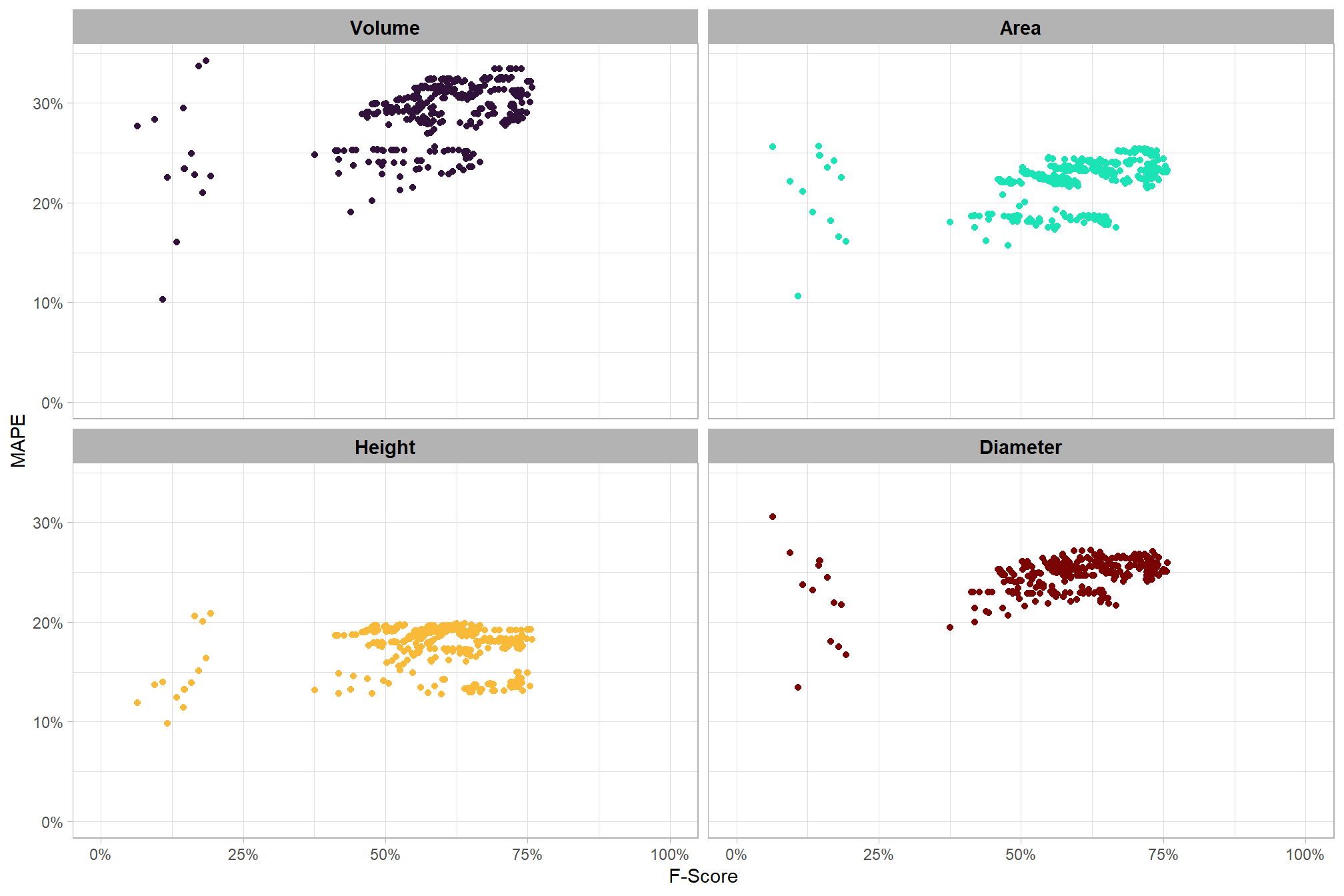
aside from a distinct cluster of points at the lower end of the F-Score range, there does not appear to be a relationship between the pile form quantification and detection accuracy metrics
let’s look at only parameter combinations that are among the best in both detection and form quantification accuracy
we’ll use the F-Score and the average rank of the MAPE metrics across all form measurements to determine the best overall list
df_temp <-
  param_combos_gt_agg %>%
  # dplyr::select(c(tidyselect::ends_with("_mape") & tidyselect::contains("volume"))) %>% names()
  dplyr::mutate(
    # label combining params
    lab = stringr::str_c(max_ht_m,max_area_m2,convexity_pct,circle_fit_iou_pct, sep = ":")
    , dplyr::across(
      .cols = c(tidyselect::ends_with("_mape"))
      # .cols = c(tidyselect::ends_with("_mape") & tidyselect::contains("volume"))
      , .fn = ~dplyr::percent_rank(-.x)
      , .names = "pct_rank_quant_{.col}"
    )
    , dplyr::across(
      .cols = c(f_score)
      # .cols = c(f_score,recall)
      , .fn = ~dplyr::percent_rank(.x)
      , .names = "pct_rank_det_{.col}"
    )
  ) %>%
  # dplyr::arrange(pct_diff_diameter_mape) %>%
  # dplyr::select(pct_diff_diameter_mape, pct_rank_pct_diff_diameter_mape) %>%
  # View()
  # now get the max of these pct ranks by row
  dplyr::rowwise() %>%
  dplyr::mutate(
    pct_rank_quant_mean = mean(
      dplyr::c_across(
        tidyselect::starts_with("pct_rank_quant_")
      )
      , na.rm = T
    )
    , pct_rank_det_mean = mean(
      dplyr::c_across(
        tidyselect::starts_with("pct_rank_det_")
      )
      , na.rm = T
    )
  ) %>%
  dplyr::ungroup() %>%
  # now make quadrant var
  dplyr::mutate(
    # this is for the quadrant plot
    overall_accuracy = dplyr::case_when(
      pct_rank_det_mean>=0.95 & pct_rank_quant_mean>=0.95 ~ 1
      , pct_rank_det_mean>=0.90 & pct_rank_quant_mean>=0.90 ~ 2
      , pct_rank_det_mean>=0.75 & pct_rank_quant_mean>=0.75 ~ 3
      , pct_rank_det_mean>=0.50 & pct_rank_quant_mean>=0.50 ~ 4
      , pct_rank_det_mean>=0.50 & pct_rank_quant_mean<0.50 ~ 5
      , pct_rank_det_mean<0.50 & pct_rank_quant_mean>=0.50 ~ 6
      , T ~ 7
    ) %>%
    factor(
      ordered = T
      , levels = 1:7
      , labels = c(
        "top 5% detection & quantification" # pct_rank_mean>=0.95 & pct_rank_f_score>=0.95 ~ 1
        , "top 10% detection & quantification" # pct_rank_mean>=0.90 & pct_rank_f_score>=0.90 ~ 2
        , "top 25% detection & quantification" # pct_rank_mean>=0.75 & pct_rank_f_score>=0.75 ~ 3
        , "top 50% detection & quantification" # pct_rank_mean>=0.50 & pct_rank_f_score>=0.50 ~ 4
        , "top 50% quantification" # pct_rank_mean>=0.50 & pct_rank_f_score<0.50 ~ 5
        , "top 50% detection" # pct_rank_mean<0.50 & pct_rank_f_score>=0.50 ~ 6
        , "bottom 50% detection & quantification"
      )
    )
  ) %>%
  dplyr::select(
    rn,max_ht_m,max_area_m2,convexity_pct,circle_fit_iou_pct
    , lab
    , f_score, recall, precision
    , tidyselect::ends_with("_mape")
    , tidyselect::starts_with("pct_rank")
    , overall_accuracy
  )

# plot
df_temp %>%
  ggplot2::ggplot(
    mapping=ggplot2::aes(x = pct_rank_det_mean, y = pct_rank_quant_mean, color = overall_accuracy)
  ) +
  ggplot2::geom_vline(xintercept = 0.5, color = "gray22") +
  ggplot2::geom_hline(yintercept = 0.5, color = "gray22") +
  ggplot2::geom_vline(xintercept = 0.75, color = "gray44") +
  ggplot2::geom_hline(yintercept = 0.75, color = "gray44") +
  ggplot2::geom_vline(xintercept = 0.9, color = "gray66") +
  ggplot2::geom_hline(yintercept = 0.9, color = "gray66") +
  ggplot2::geom_point() +
  ggplot2::scale_colour_viridis_d(option = "inferno", end = 0.8, direction = -1) +
  ggplot2::scale_x_continuous(
    labels = scales::percent_format(accuracy = 1)
    , limits = c(0,1)
  ) +
  ggplot2::scale_y_continuous(
    labels = scales::percent_format(accuracy = 1)
    , limits = c(0,1)
  ) +
  ggplot2::labs(
    x = "Percentile F-Score", y = "Percentile MAPE (mean)"
    , color = ""
  ) +
  ggplot2::theme_light() +
  ggplot2::theme(
    legend.position = "bottom"
    , legend.text = ggplot2::element_text(size = 8)
    , strip.text = ggplot2::element_text(size = 11, color = "black", face = "bold")
    , axis.text = ggplot2::element_text(size = 7)
  ) +
  ggplot2::guides(
    color = ggplot2::guide_legend(override.aes = list(shape = 15, linetype = 0, size = 5, alpha = 1))
    , shape = "none"
  )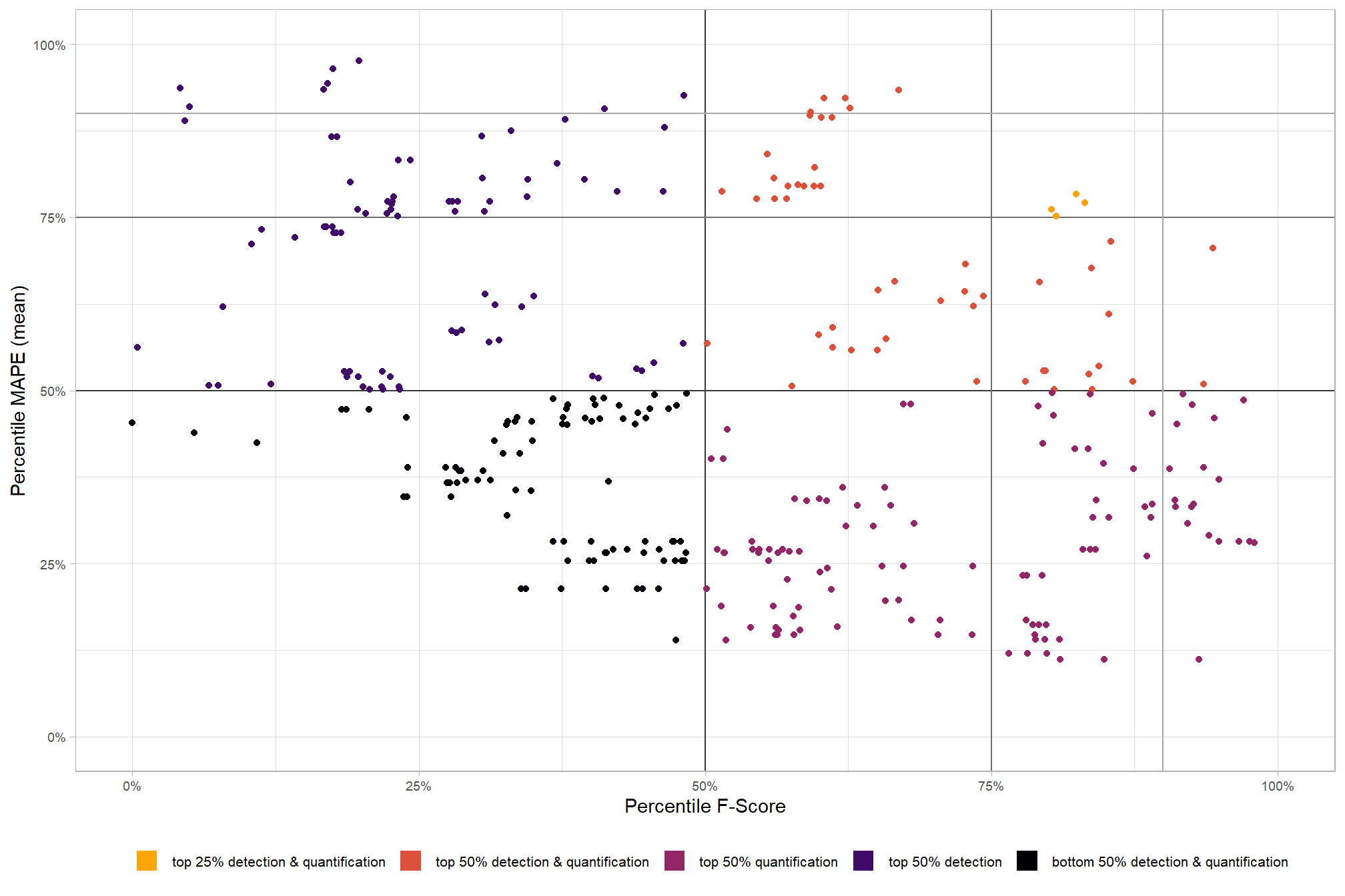
let’s look at the parameter combinations that are in the upper-right of the quadrant plot. That is, the parameter combinations that performed best at both pile detection accuracy and pile form quantification accuracy
# filter
df_temp <- df_temp %>%
  dplyr::filter(
    pct_rank_det_mean>=0.75 & pct_rank_quant_mean>=0.75
  ) %>%
  # nrow()
  dplyr::mutate(
    pct_rank_overall = (pct_rank_det_mean+pct_rank_quant_mean)/2
    , lab = forcats::fct_reorder(lab, pct_rank_overall)
  ) %>%
  dplyr::arrange(desc(pct_rank_overall)) %>%
  dplyr::mutate(rank_overall = dplyr::row_number())
# save the best overall param_combo_df record numbers
best_pile_detect_rn <- df_temp %>%
  dplyr::distinct(rn,lab,rank_overall,pct_rank_overall,pct_rank_det_mean,pct_rank_quant_mean)
# best_pile_detect_rn %>% dplyr::glimpse()
param_combos_gt_agg %>%
dplyr::ungroup() %>%
# filter for the best
dplyr::left_join(
best_pile_detect_rn %>% dplyr::distinct(rn) %>% dplyr::mutate(is_best=T)
, by = "rn"
) %>%
dplyr::mutate(is_best = dplyr::coalesce(is_best,F)) %>%
dplyr::select(
rn,max_ht_m,max_area_m2,convexity_pct,circle_fit_iou_pct
, is_best
, f_score
# quantification accuracy
, tidyselect::ends_with("_mape")
) %>%
tidyr::pivot_longer(
cols = c(tidyselect::ends_with("_mape"))
, names_to = "metric"
, values_to = "value"
) %>%
dplyr::mutate(
eval_metric = stringr::str_extract(metric, "(_rmse|_rrmse|_mean|_mape)$") %>%
stringr::str_remove_all("_") %>%
stringr::str_replace_all("mean","me") %>%
toupper() %>%
factor(
ordered = T
, levels = c("ME","RMSE","RRMSE","MAPE")
)
, pile_metric = metric %>%
stringr::str_remove("(_rmse|_rrmse|_mean|_mape)$") %>%
stringr::str_extract("(paraboloid_volume|volume|area|height|diameter)") %>%
factor(
ordered = T
, levels = c(
"volume"
, "paraboloid_volume"
, "area"
, "height"
, "diameter"
)
, labels = c(
"Volume"
, "Volume paraboloid"
, "Area"
, "Height"
, "Diameter"
)
)
, color_metric = ifelse(is_best, pile_metric, NA) %>% factor()
) %>%
dplyr::arrange(is_best) %>%
# plot
ggplot2::ggplot(mapping = ggplot2::aes(x = f_score, y = value, color = color_metric)) +
ggplot2::geom_point() +
ggplot2::facet_wrap(facets = dplyr::vars(pile_metric)) +
ggplot2::scale_color_viridis_d(option = "turbo", na.value = "gray88") +
ggplot2::scale_x_continuous(
labels = scales::percent_format(accuracy = 1)
, limits = c(0,1)
) +
ggplot2::scale_y_continuous(
labels = scales::percent_format(accuracy = 1)
, limits = c(0,NA)
) +
ggplot2::labs(x = "F-Score", y = "MAPE", caption = "*records in gray not selected") +
ggplot2::theme_light() +
ggplot2::theme(
legend.position = "none"
, strip.text = ggplot2::element_text(size = 11, color = "black", face = "bold")
)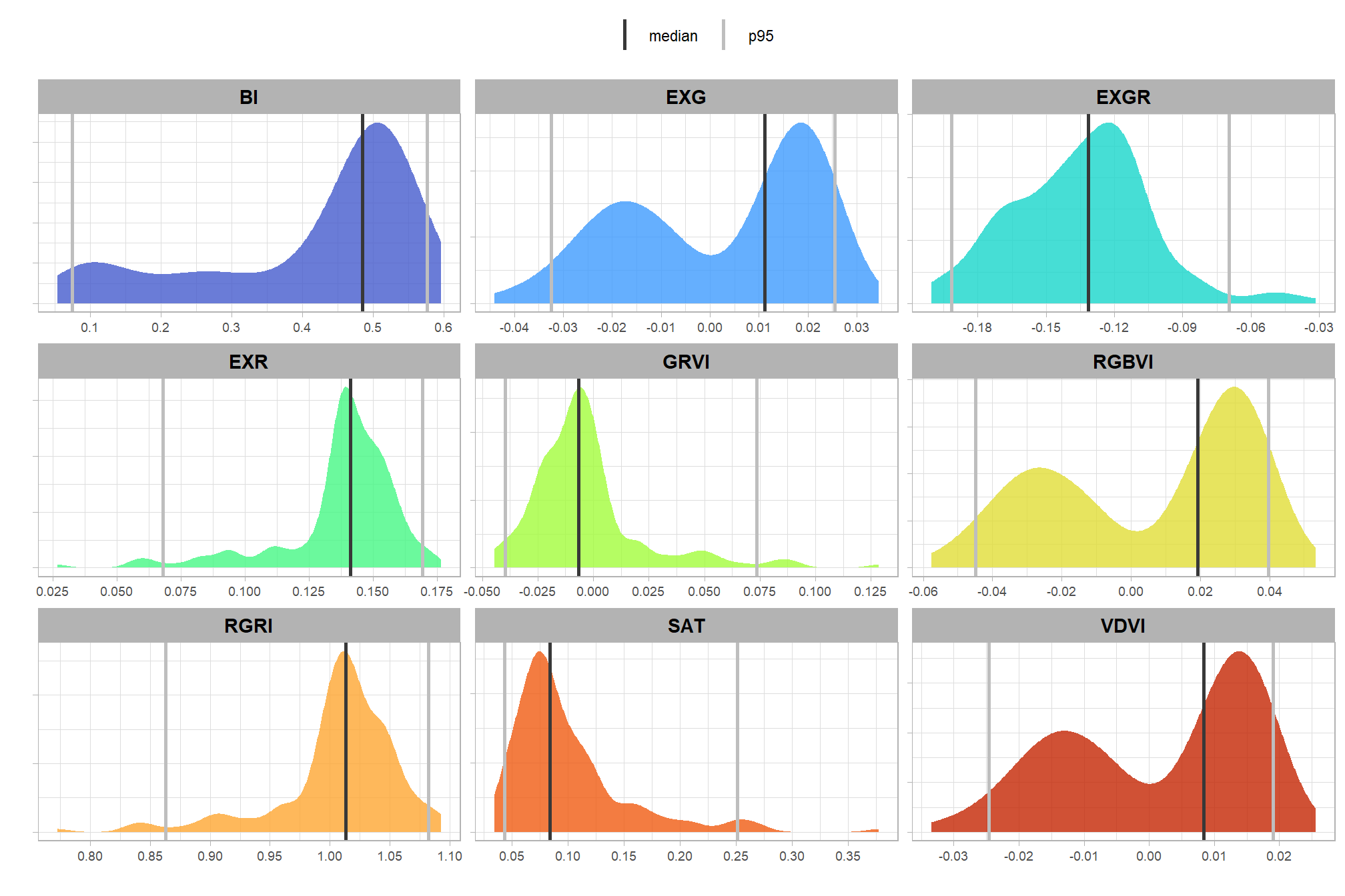
if we look at these top parameter combinations only, what can we expect regarding detection accuracy
# plot it
plt_detection_dist(
  df = param_combos_gt_agg %>%
    # filter for best of best
    dplyr::inner_join(
      best_pile_detect_rn %>% dplyr::distinct(rn)
      , by = "rn"
    )
  , paste0(
   "distribution of pile detection accuracy metrics for the top"
   , " (n="
   , scales::comma(nrow(best_pile_detect_rn), accuracy = 1)
   , ") "
   , "parameter combinations\nbased on both detection and quantification accuracy"
  )
)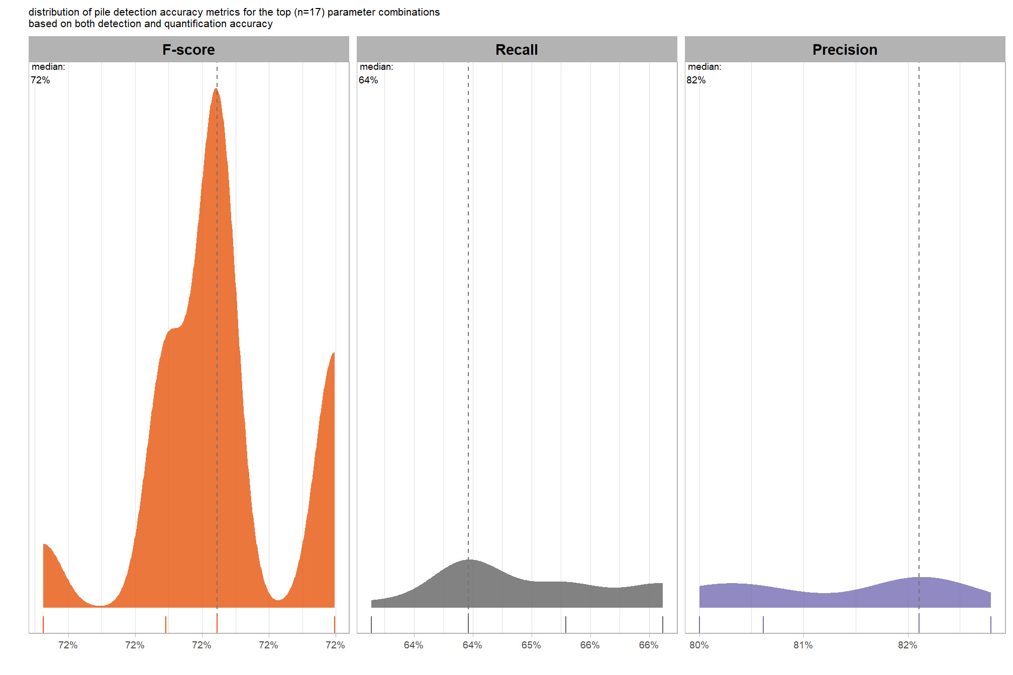
this is interesting, among the top performers in both detection (F-score) and quantification (overall MAPE), a few combinations had noticeably higher recall rates. assuming quantification accuracy is similar across this elite group, we should prioritize those with the highest recall.
but first, if we look at all these top combinations, what can we expect regarding their quantification accuracy?
# plot it
plt_form_quantification_dist(
  df = param_combos_gt_agg %>%
    dplyr::ungroup() %>%
    # filter for best of best
    dplyr::inner_join(
      best_pile_detect_rn %>% dplyr::distinct(rn)
      , by = "rn"
    )
  , paste0(
     "distribution of pile form quantification accuracy metrics for the top"
     # , scales::percent(1-pct_rank_th_top,accuracy=1)
     , " (n="
     , scales::comma(nrow(best_pile_detect_rn), accuracy = 1)
     , ") "
     , "parameter combinations\nbased on both detection and quantification accuracy"
  )
)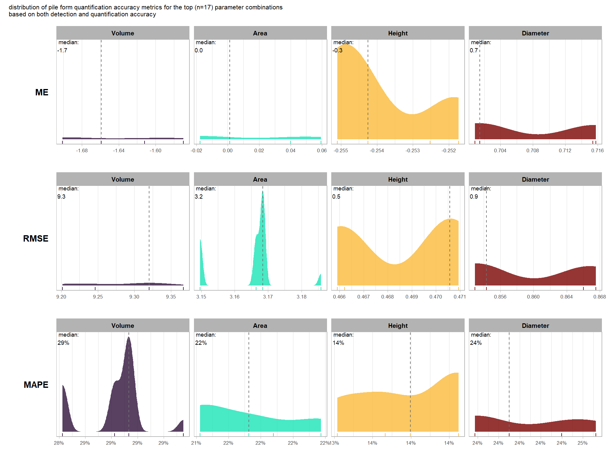
the distributions of these form quantification accuracy metrics span a narrow range (x-axis), especially with respect to MAPE. as such, we’ll focus on the best overall parameter combinations that also achieved the highest recall rates
6.4 Final recommended settings
our final step in this sensitivity testing is to identify the best-performing parameter combinations that not only balance detection and quantification accuracy but also achieve the highest recall rates. we’ll select these by choosing any combination whose recall rate is at least one standard deviation above the average for this top group. if no combinations meet this criterion, we will instead select the top 10 combinations based on their recall rates.
# put a flag in our best_pile_detect_rn data
best_pile_detect_rn <-
  best_pile_detect_rn %>%
  dplyr::left_join(
    param_combos_gt_agg %>%
      dplyr::ungroup() %>%
      # filter for best of best
      dplyr::inner_join(
        best_pile_detect_rn %>% dplyr::distinct(rn)
        , by = "rn"
      ) %>%
      # check recall rate
      dplyr::arrange(desc(recall)) %>%
      dplyr::mutate(
        is_recall_above_mean = recall >= ( mean(recall) + sd(recall)*1.5 )
        # if no records have a recall at least one stdandard dev above the mean, just take the top ten
        , is_top_recall = dplyr::case_when(
          sum(is_recall_above_mean)>4 ~ is_recall_above_mean
          , T ~ dplyr::row_number()<=10
        )
      ) %>%
      dplyr::select(rn,is_top_recall)
    , by = "rn"
  )
# huh?
# best_pile_detect_rn %>% dplyr::glimpse()
best_pile_detect_rn %>% dplyr::count(is_top_recall)
## # A tibble: 2 × 2
## is_top_recall n
## <lgl> <int>
## 1 FALSE 7
## 2 TRUE 10finally, let’s look at the pile detection accuracy metrics at the individual parameter combination level
# pal_temp %>% scales::show_col()
# filter and reshape
df_temp <-
  param_combos_gt_agg %>%
  dplyr::inner_join(
    best_pile_detect_rn %>% dplyr::filter(is_top_recall) %>%
      dplyr::select(rn,lab,rank_overall)
    , by = "rn"
  ) %>%
  dplyr::select(
    max_ht_m,max_area_m2,convexity_pct,circle_fit_iou_pct
    , lab
    # detection
    , f_score, recall, precision
    # quantification
    , tidyselect::ends_with("_rmse")
    , tidyselect::ends_with("_rrmse")
    , tidyselect::ends_with("_mean")
    , tidyselect::ends_with("_mape")
  ) %>%
  tidyr::pivot_longer(
    cols = c(
      f_score, recall, precision
      , tidyselect::ends_with("_rmse")
      , tidyselect::ends_with("_rrmse")
      , tidyselect::ends_with("_mean")
      , tidyselect::ends_with("_mape")
    )
    , names_to = "metric"
    , values_to = "value"
  ) %>%
  dplyr::mutate(
    eval_metric = stringr::str_extract(metric, "(_rmse|_rrmse|_mean|_mape|f_score|recall|precision)$") %>%
      stringr::str_remove_all("_") %>%
      stringr::str_replace_all("mean","me") %>%
      toupper() %>%
      factor(
        ordered = T
        , levels = c("FSCORE","RECALL","PRECISION", "ME","RMSE","RRMSE","MAPE")
        , labels = c("F-score","Recall","Precision", "ME","RMSE","RRMSE","MAPE")
      )
    , pile_metric = metric %>%
      stringr::str_remove("(_rmse|_rrmse|_mean|_mape)$") %>%
      stringr::str_extract("(paraboloid_volume|volume|area|height|diameter)") %>%
      dplyr::coalesce("detection") %>%
      factor(
        ordered = T
        , levels = c(
          "detection"
          , "volume"
          , "paraboloid_volume"
          , "area"
          , "height"
          , "diameter"
        )
        , labels = c(
          "Detection"
          , "Volume"
          , "Volume paraboloid"
          , "Area"
          , "Height"
          , "Diameter"
        )
      )
    , value_lab = dplyr::case_when(
        eval_metric %in% c("F-score","Recall","Precision", "RRMSE", "MAPE") ~ scales::percent(value,accuracy=0.1)
        , eval_metric == "ME" ~ scales::comma(value,accuracy=0.01)
        , T ~ scales::comma(value,accuracy=0.1)
      )
  ) %>%
  # make var for color
  dplyr::group_by(pile_metric, eval_metric) %>%
  dplyr::mutate(
    # for ME, color by abs...for f-score,recall,precision color by -value so that higher means better...
      # ...since higher means worse for quantification accuracy metrics
    value_dir = dplyr::case_when(
      eval_metric %in% c("ME") ~ abs(value)
      , eval_metric %in% c("F-score","Recall","Precision") ~ -value
      , T ~ value
    )
    , value_z = (value_dir-mean(value_dir,na.rm=T))/sd(value_dir,na.rm=T) # this is the key to the different colors within facets
  ) %>%
  dplyr::ungroup()

# how to plot all of this (without patchwork)?????
df_temp %>%
  dplyr::filter(!eval_metric %in% c("RRMSE")) %>%
  # View()
  ggplot2::ggplot(mapping = ggplot2::aes(x = eval_metric, y = lab)) +
  ggplot2::geom_tile(
    mapping = ggplot2::aes(fill = pile_metric, alpha = -value_z)
    , color = "gray"
  ) +
  ggplot2::geom_text(
    mapping = ggplot2::aes(label = value_lab, fontface = "bold")
    , color = "white"
  ) +
  ggplot2::facet_grid(cols = dplyr::vars(pile_metric), scales = "free_x") +
  ggplot2::scale_x_discrete(position = "top") +
  ggplot2::scale_fill_manual(values = c("gray33", viridis::turbo(n=4))) +
  ggplot2::scale_alpha_binned(range = c(0.55, 1)) + # this is the key to the different colors within facets
  ggplot2::theme_light() +
  ggplot2::labs(
    x = ""
    , y = "max_ht_m : max_area_m2 : convexity_pct : circle_fit_iou_pct"
    , subtitle = paste0(
       "pile detection and form quantification accuracy metrics for the top"
       # , scales::percent(1-pct_rank_th_top,accuracy=1)
       , " (n="
       , scales::comma(sum(best_pile_detect_rn$is_top_recall,na.rm=T), accuracy = 1)
       , ") "
       , "overall parameter combinations\nbased on both detection and quantification accuracy"
      )
    , caption = "*darker colors indicate relatively higher accuracy values"
  ) +
  ggplot2::theme(
    legend.position = "none"
    , panel.grid = ggplot2::element_blank()
    , strip.placement = "outside"
    , strip.text.x = ggplot2::element_text(size = 8, color = "black", face = "bold")
    , axis.text.x = ggplot2::element_text(size = 7, color = "black", face = "bold")
    , axis.title.x = ggplot2::element_blank()
    , plot.subtitle = ggplot2::element_text(size = 8)
  )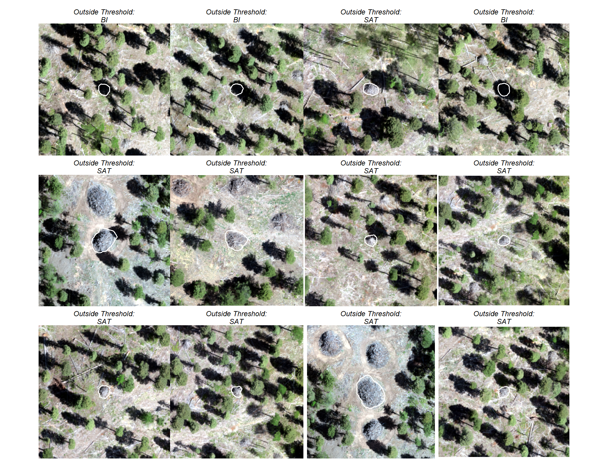
this plot allows for a simultaneous comparison of all metrics for pile detection and pile form quantification. it includes only the parameter combinations that achieved the best balanced accuracy, helping users identify the optimal settings by evaluating the trade-offs between detection and form quantification.
let’s table this
param_combos_gt_agg %>%
  dplyr::inner_join(
    best_pile_detect_rn %>% dplyr::filter(is_top_recall) %>%
      dplyr::select(rn,lab,rank_overall)
    , by = "rn"
  ) %>%
  # first select to arrange eval_metric
  dplyr::select(
    lab
    , max_ht_m,max_area_m2,convexity_pct,circle_fit_iou_pct
    # detection
    , f_score, recall, precision
    # quantification
    , tidyselect::ends_with("_mean")
    , tidyselect::ends_with("_rmse")
    # , tidyselect::ends_with("_rrmse")
    , tidyselect::ends_with("_mape")
  ) %>%
  # second select to arrange pile_metric
  dplyr::select(
    lab
    , max_ht_m,max_area_m2,convexity_pct,circle_fit_iou_pct
    # detection
    , f_score, recall, precision
    # quantification
    , c(tidyselect::contains("volume") & !tidyselect::contains("paraboloid"))
    , tidyselect::contains("area")
    , tidyselect::contains("height")
    , tidyselect::contains("diameter")
  ) %>%
  # names()
  dplyr::mutate(
    dplyr::across(
      .cols = c(f_score, recall, precision, tidyselect::ends_with("_mape"))
      , .fn = ~ scales::percent(.x, accuracy = 1)
    )
    , dplyr::across(
      .cols = c(tidyselect::ends_with("_mean"))
      , .fn = ~ scales::comma(.x, accuracy = 0.01)
    )
    , dplyr::across(
      .cols = c(tidyselect::ends_with("_rmse"))
      , .fn = ~ scales::comma(.x, accuracy = 0.1)
    )
  ) %>%
  dplyr::mutate(blank= "   " ) %>%
  dplyr::relocate(blank, .before = f_score) %>%
  dplyr::arrange(desc(lab)) %>%
  kableExtra::kbl(
    caption = paste0(
       "pile detection and form quantification accuracy metrics for the final recommended parameter settings"
       # , scales::percent(1-pct_rank_th_top,accuracy=1)
       , " (n="
       , scales::comma(sum(best_pile_detect_rn$is_top_recall,na.rm=T), accuracy = 1)
       , ")"
      )
    , col.names = c(
      ""
      ,"max_ht_m","max_area_m2","convexity_pct","circle_fit_iou_pct"
      , "   "
      , "F-score", "Recall", "Precision"
      , rep(c("ME","RMSE","MAPE"), times = 4)
    )
    , escape = F
  ) %>%
  kableExtra::kable_styling(font_size = 11) %>%
  kableExtra::add_header_above(c(
    " "=6
    , "Detection" = 3
    , "Volume" = 3
    , "Area" = 3
    , "Height" = 3
    , "Diameter" = 3
  )) %>%
  kableExtra::column_spec(seq(6,21,by=3), border_right = TRUE, include_thead = TRUE) %>%
  kableExtra::column_spec(
    column = 7:21
    , extra_css = "font-size: 10px;"
    , include_thead = T
  ) %>%
kableExtra::scroll_box(width = "740px") | max_ht_m | max_area_m2 | convexity_pct | circle_fit_iou_pct | F-score | Recall | Precision | ME | RMSE | MAPE | ME | RMSE | MAPE | ME | RMSE | MAPE | ME | RMSE | MAPE | ||
|---|---|---|---|---|---|---|---|---|---|---|---|---|---|---|---|---|---|---|---|---|
| 2:40:0.7:0.5 | 2 | 40 | 0.7 | 0.5 | 72% | 64% | 82% | -1.70 | 9.3 | 29% | -0.02 | 3.2 | 21% | -0.26 | 0.5 | 14% | 0.70 | 0.9 | 24% | |
| 2:30:0.7:0.5 | 2 | 30 | 0.7 | 0.5 | 72% | 64% | 82% | -1.70 | 9.3 | 29% | -0.02 | 3.2 | 21% | -0.26 | 0.5 | 14% | 0.70 | 0.9 | 24% | |
| 2:30:0.6:0.5 | 2 | 30 | 0.6 | 0.5 | 72% | 66% | 80% | -1.61 | 9.2 | 28% | 0.04 | 3.1 | 22% | -0.25 | 0.5 | 14% | 0.72 | 0.9 | 24% | |
| 2:30:0.5:0.5 | 2 | 30 | 0.5 | 0.5 | 72% | 66% | 80% | -1.61 | 9.2 | 28% | 0.04 | 3.1 | 22% | -0.25 | 0.5 | 14% | 0.72 | 0.9 | 24% | |
| 2:30:0.4:0.5 | 2 | 30 | 0.4 | 0.5 | 72% | 66% | 80% | -1.61 | 9.2 | 28% | 0.04 | 3.1 | 22% | -0.25 | 0.5 | 14% | 0.72 | 0.9 | 24% | |
| 2:30:0.3:0.5 | 2 | 30 | 0.3 | 0.5 | 72% | 66% | 80% | -1.61 | 9.2 | 28% | 0.04 | 3.1 | 22% | -0.25 | 0.5 | 14% | 0.72 | 0.9 | 24% | |
| 2:20:0.6:0.5 | 2 | 20 | 0.6 | 0.5 | 72% | 65% | 81% | -1.57 | 9.2 | 29% | 0.06 | 3.2 | 22% | -0.25 | 0.5 | 13% | 0.72 | 0.9 | 25% | |
| 2:20:0.5:0.5 | 2 | 20 | 0.5 | 0.5 | 72% | 65% | 81% | -1.57 | 9.2 | 29% | 0.06 | 3.2 | 22% | -0.25 | 0.5 | 13% | 0.72 | 0.9 | 25% | |
| 2:20:0.4:0.5 | 2 | 20 | 0.4 | 0.5 | 72% | 65% | 81% | -1.57 | 9.2 | 29% | 0.06 | 3.2 | 22% | -0.25 | 0.5 | 13% | 0.72 | 0.9 | 25% | |
| 2:20:0.3:0.5 | 2 | 20 | 0.3 | 0.5 | 72% | 65% | 81% | -1.57 | 9.2 | 29% | 0.06 | 3.2 | 22% | -0.25 | 0.5 | 13% | 0.72 | 0.9 | 25% |
what is the detection accuracy of these final recommended parameter settings?
# plot it
plt_detection_dist(
  df = param_combos_gt_agg %>%
    # filter for best of best
    dplyr::inner_join(
      best_pile_detect_rn %>% dplyr::filter(is_top_recall) %>% dplyr::distinct(rn)
      , by = "rn"
    )
  , paste0(
       "distribution of pile detection accuracy metrics for the final recommended parameter settings"
       # , scales::percent(1-pct_rank_th_top,accuracy=1)
       , " (n="
       , scales::comma(sum(best_pile_detect_rn$is_top_recall,na.rm=T), accuracy = 1)
       , ")"
      )
)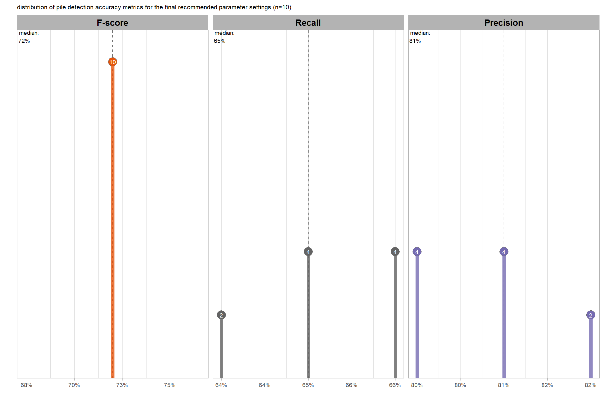
what is the quantification accuracy of these final recommended parameter settings?
# plot it
plt_form_quantification_dist(
  df = param_combos_gt_agg %>%
    # filter for best of best
    dplyr::inner_join(
      best_pile_detect_rn %>% dplyr::filter(is_top_recall) %>% dplyr::distinct(rn)
      , by = "rn"
    )
  , paste0(
       "distribution of pile form quantification accuracy metrics for the final recommended parameter settings"
       # , scales::percent(1-pct_rank_th_top,accuracy=1)
       , " (n="
       , scales::comma(sum(best_pile_detect_rn$is_top_recall,na.rm=T), accuracy = 1)
       , ")"
      )
)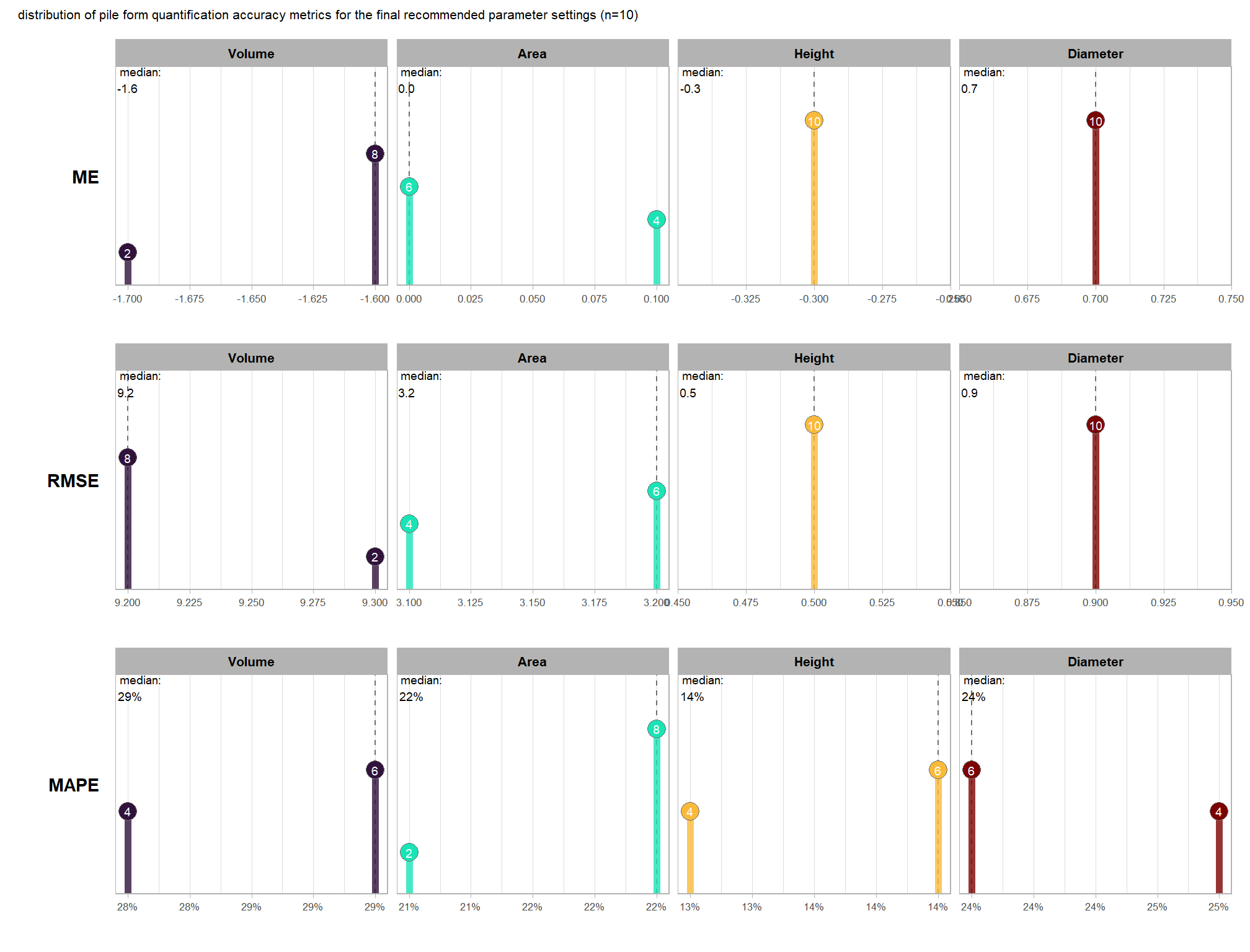
6.5 Appendix: Parameter combination drill-downs
The objective of these combination drill-down plots is to convey the pile detection evaluation results for a given set of the convexity_pct, circle_fit_iou_pct, and max_area_m2 parameter settings while holding the max_ht_m and min_area_m2 parameters constant since these should be defined based on the expected values of the treatment area. Based on our validation data, it was clear that the optimal max_ht_m value was 3.0 and that setting the value above this level resulted in understory trees being incorrectly detected as slash piles.
6.5.1 F-score
param_combos_gt_agg %>%
  dplyr::filter(
    max_ht_m == best_max_ht_m_temp
    & min_area_m2 == best_min_area_m2_temp
  ) %>%
  dplyr::mutate(
    flab = stringr::str_c("max_area_m2",max_area_m2,sep = " = ") %>%
      forcats::fct_reorder(max_area_m2)
  ) %>%
  ggplot2::ggplot(mapping = ggplot2::aes(
      y = as.factor(convexity_pct)
      , x = as.factor(circle_fit_iou_pct)
      , fill = f_score
      , label = scales::percent(f_score,accuracy = 1)
    )) +
    ggplot2::geom_tile(color = "white") +
    ggplot2::geom_text(color = "white", size = 3) +
    ggplot2::facet_wrap(facets = dplyr::vars(flab)) +
    ggplot2::scale_fill_distiller(
      palette = "Oranges"
      , direction = 1
      , labels = scales::percent_format(accuracy = 1)
      , limits = c(0,1)
    ) +
    labs(
      x = "circle_fit_iou_pct"
      , y = "convexity_pct"
      , subtitle = "F-score by parameter setting combination levels"
    ) +
    theme_light() +
    theme(
      legend.position = "none"
      , axis.text.x = element_text(angle = 90, vjust = 0.5, hjust = 1)
      , panel.background = element_blank()
      , panel.grid = element_blank()
      # , plot.title = element_text(hjust = 0.5)
      # , plot.subtitle = element_text(hjust = 0.5)
      , strip.text = element_text(color = "black", face = "bold")
    )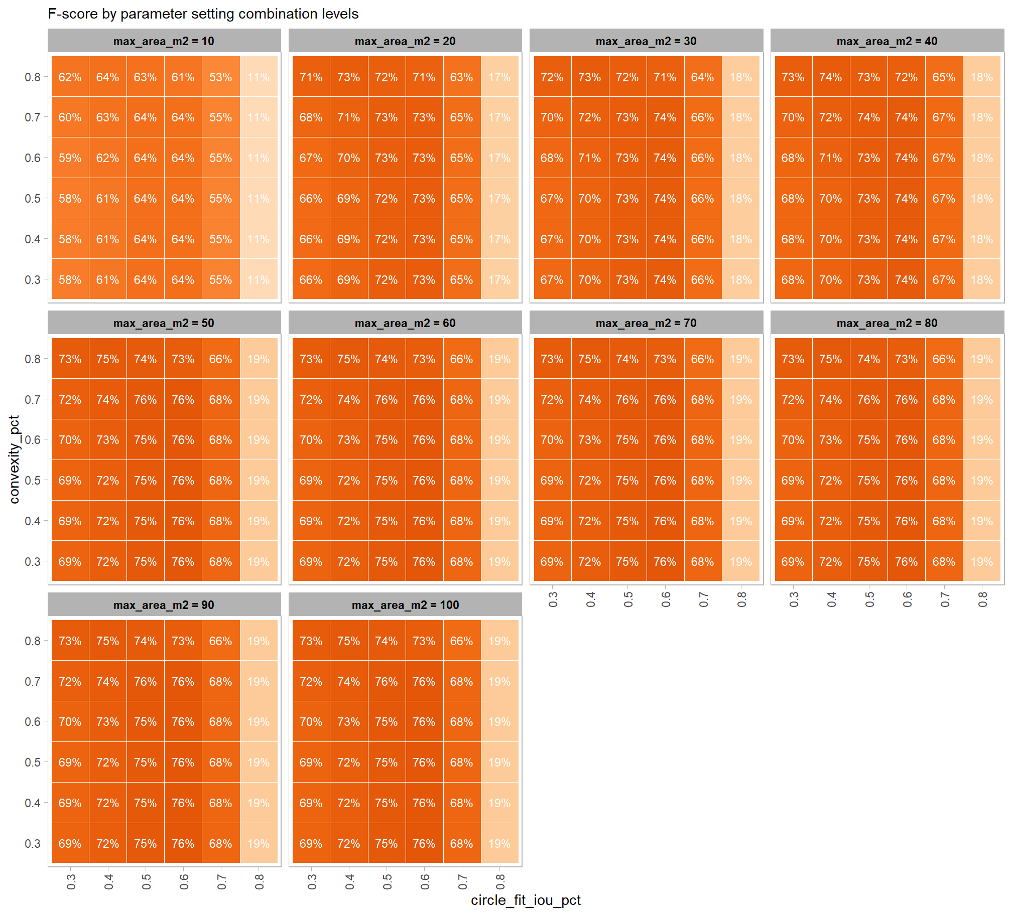
6.5.2 Recall
param_combos_gt_agg %>%
  dplyr::filter(
    max_ht_m == best_max_ht_m_temp
    & min_area_m2 == best_min_area_m2_temp
  ) %>%
  dplyr::mutate(
    flab = stringr::str_c("max_area_m2",max_area_m2,sep = " = ") %>%
      forcats::fct_reorder(max_area_m2)
  ) %>%
  ggplot2::ggplot(mapping = ggplot2::aes(
      y = as.factor(convexity_pct)
      , x = as.factor(circle_fit_iou_pct)
      , fill = recall
      , label = scales::percent(recall,accuracy = 1)
    )) +
    ggplot2::geom_tile(color = "white") +
    ggplot2::geom_text(color = "white", size = 3) +
    ggplot2::facet_wrap(facets = dplyr::vars(flab)) +
    ggplot2::scale_fill_gradient(
      low = "gray97", high = "gray27"
      , labels = scales::percent_format(accuracy = 1)
      , limits = c(0,1)
    ) +
    labs(
      x = "circle_fit_iou_pct"
      , y = "convexity_pct"
      , subtitle = "Recall by parameter setting combination levels"
    ) +
    theme_light() +
    theme(
      legend.position = "none"
      , axis.text.x = element_text(angle = 90, vjust = 0.5, hjust = 1)
      , panel.background = element_blank()
      , panel.grid = element_blank()
      # , plot.title = element_text(hjust = 0.5)
      # , plot.subtitle = element_text(hjust = 0.5)
      , strip.text = element_text(color = "black", face = "bold")
    )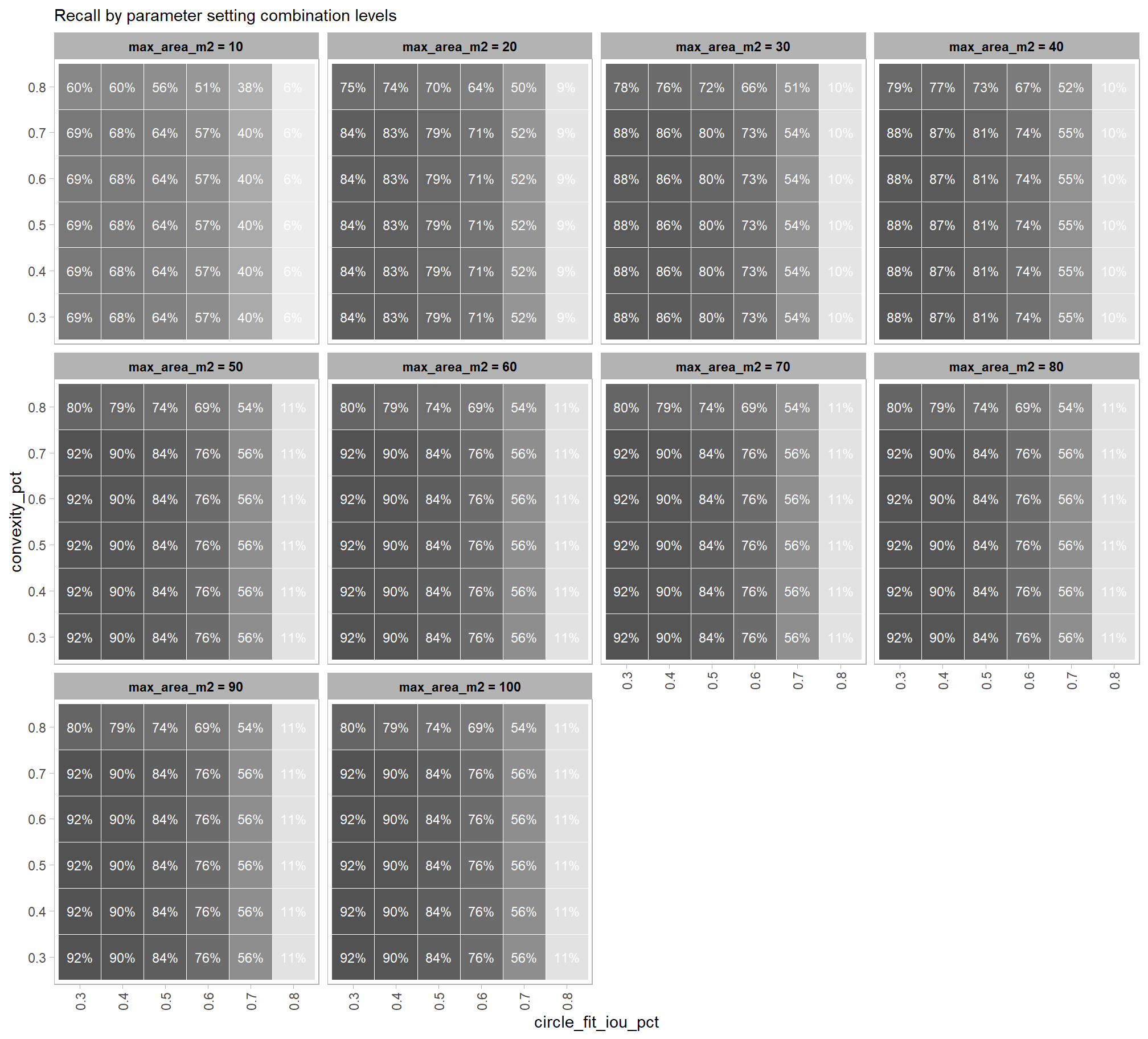
6.5.3 Precision
param_combos_gt_agg %>%
  dplyr::filter(
    max_ht_m == best_max_ht_m_temp
    & min_area_m2 == best_min_area_m2_temp
  ) %>%
  dplyr::mutate(
    flab = stringr::str_c("max_area_m2",max_area_m2,sep = " = ") %>%
      forcats::fct_reorder(max_area_m2)
  ) %>%
  ggplot2::ggplot(mapping = ggplot2::aes(
      y = as.factor(convexity_pct)
      , x = as.factor(circle_fit_iou_pct)
      , fill = precision
      , label = scales::percent(precision,accuracy = 1)
    )) +
    ggplot2::geom_tile(color = "white") +
    ggplot2::geom_text(color = "white", size = 3) +
    ggplot2::facet_wrap(facets = dplyr::vars(flab)) +
    ggplot2::scale_fill_distiller(
      palette = "Purples"
      , direction = 1
      , labels = scales::percent_format(accuracy = 1)
      , limits = c(0,1)
    ) +
    labs(
      x = "circle_fit_iou_pct"
      , y = "convexity_pct"
      , subtitle = "Precision by parameter setting combination levels"
    ) +
    theme_light() +
    theme(
      legend.position = "none"
      , axis.text.x = element_text(angle = 90, vjust = 0.5, hjust = 1)
      , panel.background = element_blank()
      , panel.grid = element_blank()
      # , plot.title = element_text(hjust = 0.5)
      # , plot.subtitle = element_text(hjust = 0.5)
      , strip.text = element_text(color = "black", face = "bold")
    )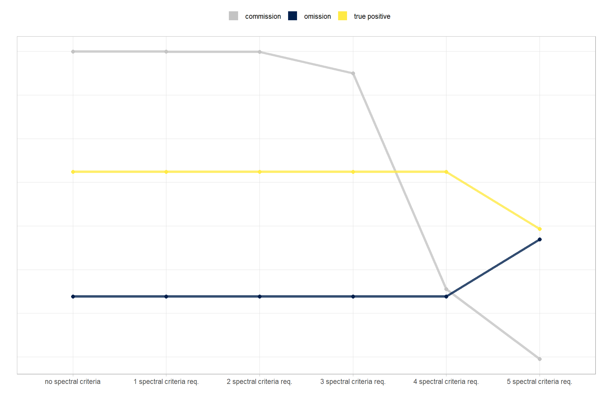
6.5.4 MAPE Volume irregular
param_combos_gt_agg %>%
  dplyr::filter(
    max_ht_m == best_max_ht_m_temp
    & min_area_m2 == best_min_area_m2_temp
  ) %>%
  dplyr::mutate(
    flab = stringr::str_c("max_area_m2",max_area_m2,sep = " = ") %>%
      forcats::fct_reorder(max_area_m2)
  ) %>%
  ggplot2::ggplot(mapping = ggplot2::aes(
      y = as.factor(convexity_pct)
      , x = as.factor(circle_fit_iou_pct)
      # , fill = pct_diff_volume_field_mape
      , label = scales::percent(pct_diff_volume_field_mape,accuracy = 1)
    )) +
    ggplot2::geom_tile(mapping = ggplot2::aes(alpha = -pct_diff_volume_field_mape), color = "white", fill = viridis::turbo(n=4)[1]) +
    ggplot2::geom_text(color = "white", size = 3) +
    ggplot2::facet_wrap(facets = dplyr::vars(flab)) +
    ggplot2::scale_alpha_binned(range = c(0.4,1)) +
    labs(
      x = "circle_fit_iou_pct"
      , y = "convexity_pct"
      , subtitle = "MAPE field-collected volume versus irregular form prediction volume by parameter setting combination levels"
    ) +
    theme_light() +
    theme(
      legend.position = "none"
      , axis.text.x = element_text(angle = 90, vjust = 0.5, hjust = 1)
      , panel.background = element_blank()
      , panel.grid = element_blank()
      # , plot.title = element_text(hjust = 0.5)
      # , plot.subtitle = element_text(hjust = 0.5)
      , strip.text = element_text(color = "black", face = "bold")
    )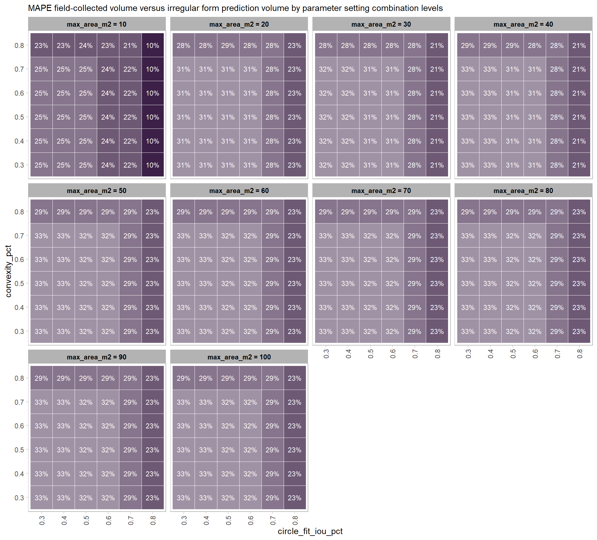
6.5.5 MAPE Diameter
param_combos_gt_agg %>%
  dplyr::filter(
    max_ht_m == best_max_ht_m_temp
    & min_area_m2 == best_min_area_m2_temp
  ) %>%
  dplyr::mutate(
    flab = stringr::str_c("max_area_m2",max_area_m2,sep = " = ") %>%
      forcats::fct_reorder(max_area_m2)
  ) %>%
  ggplot2::ggplot(mapping = ggplot2::aes(
      y = as.factor(convexity_pct)
      , x = as.factor(circle_fit_iou_pct)
      , label = scales::percent(pct_diff_diameter_mape,accuracy = 1)
    )) +
    ggplot2::geom_tile(mapping = ggplot2::aes(alpha = -pct_diff_diameter_mape), color = "white", fill = viridis::turbo(n=4)[2]) +
    ggplot2::geom_text(color = "black", size = 3) +
    ggplot2::facet_wrap(facets = dplyr::vars(flab)) +
    ggplot2::scale_alpha_binned(range = c(0.4,1)) +
    labs(
      x = "circle_fit_iou_pct"
      , y = "convexity_pct"
      , subtitle = "MAPE field-collected diameter versus prediction diameter by parameter setting combination levels"
    ) +
    theme_light() +
    theme(
      legend.position = "none"
      , axis.text.x = element_text(angle = 90, vjust = 0.5, hjust = 1)
      , panel.background = element_blank()
      , panel.grid = element_blank()
      # , plot.title = element_text(hjust = 0.5)
      # , plot.subtitle = element_text(hjust = 0.5)
      , strip.text = element_text(color = "black", face = "bold")
    )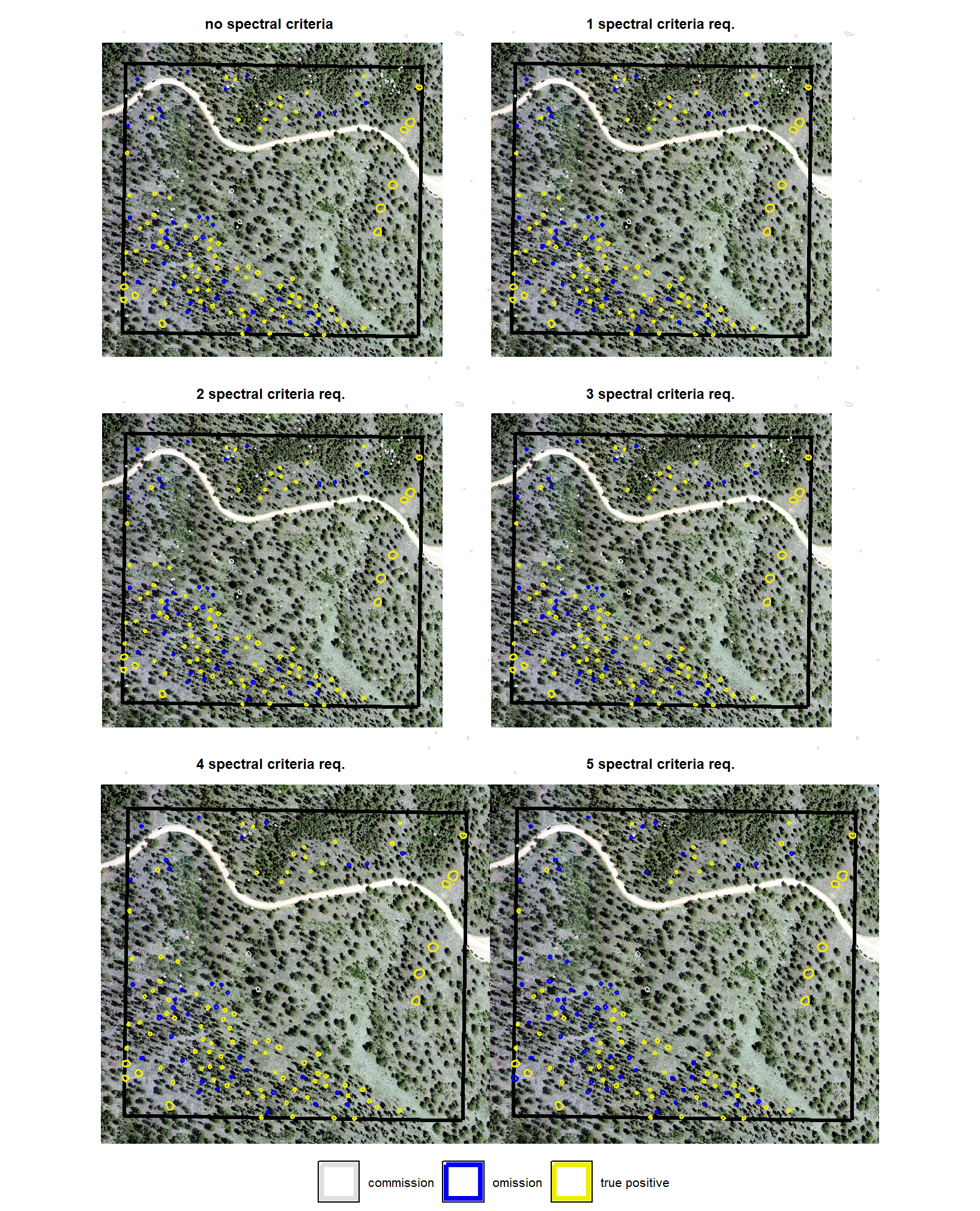
6.5.6 MAPE Area
param_combos_gt_agg %>%
  dplyr::filter(
    max_ht_m == best_max_ht_m_temp
    & min_area_m2 == best_min_area_m2_temp
  ) %>%
  dplyr::mutate(
    flab = stringr::str_c("max_area_m2",max_area_m2,sep = " = ") %>%
      forcats::fct_reorder(max_area_m2)
  ) %>%
  ggplot2::ggplot(mapping = ggplot2::aes(
      y = as.factor(convexity_pct)
      , x = as.factor(circle_fit_iou_pct)
      # , fill = pct_diff_area_field_mape
      , label = scales::percent(pct_diff_area_field_mape,accuracy = 1)
    )) +
    ggplot2::geom_tile(mapping = ggplot2::aes(alpha = -pct_diff_area_field_mape), color = "white", fill = viridis::turbo(n=4)[3]) +
    ggplot2::geom_text(color = "black", size = 3) +
    ggplot2::facet_wrap(facets = dplyr::vars(flab)) +
    ggplot2::scale_alpha_binned(range = c(0.4,1)) +
    # ggplot2::scale_fill_distiller(
    #   palette = "YlGn"
    #   , direction = 1
    #   , labels = scales::percent_format(accuracy = 1)
    #   , limits = c(0,1)
    # ) +
    labs(
      x = "circle_fit_iou_pct"
      , y = "convexity_pct"
      , subtitle = "MAPE field-collected area versus prediction area by parameter setting combination levels"
    ) +
    theme_light() +
    theme(
      legend.position = "none"
      , axis.text.x = element_text(angle = 90, vjust = 0.5, hjust = 1)
      , panel.background = element_blank()
      , panel.grid = element_blank()
      # , plot.title = element_text(hjust = 0.5)
      # , plot.subtitle = element_text(hjust = 0.5)
      , strip.text = element_text(color = "black", face = "bold")
    )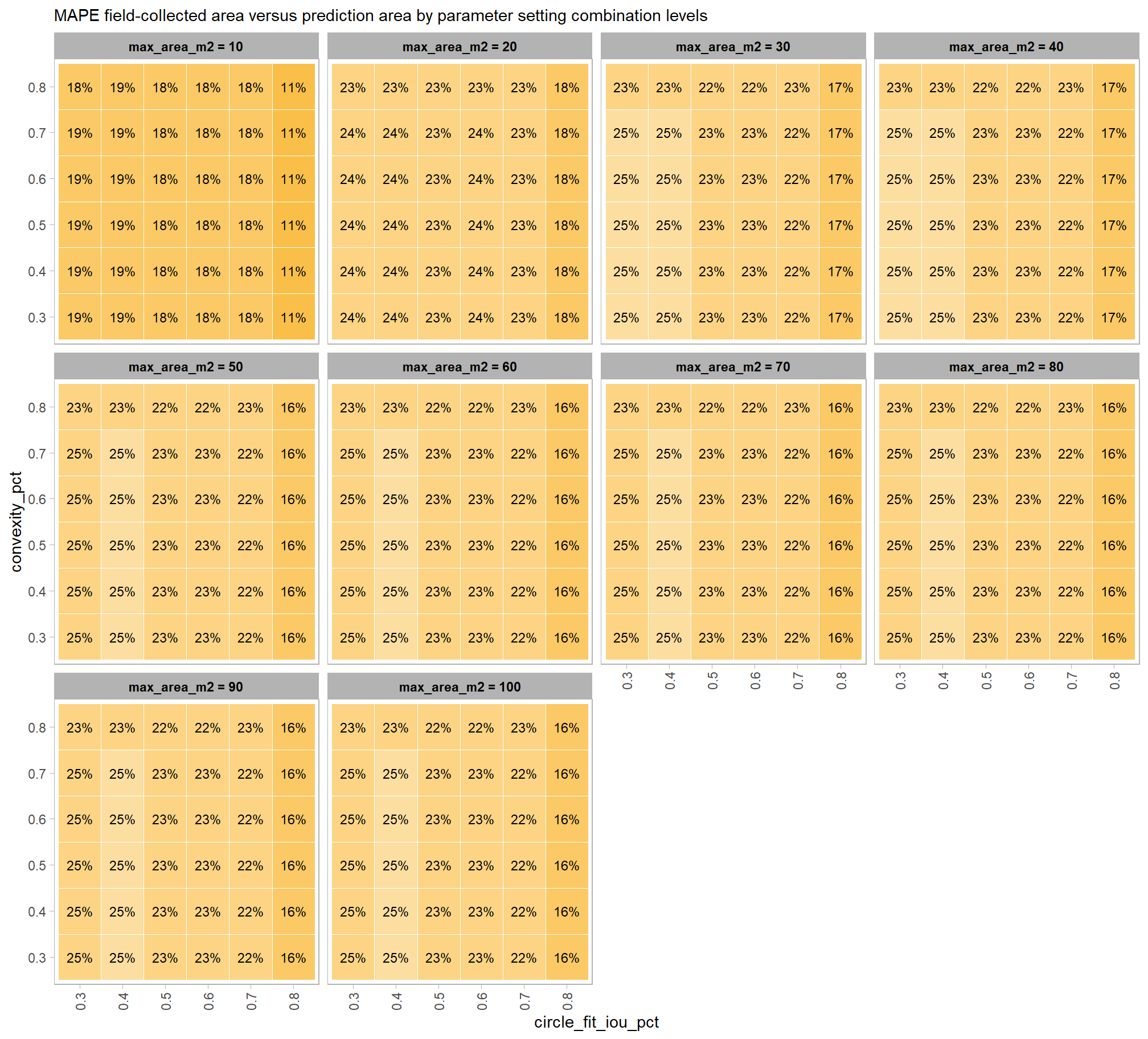
6.5.7 MAPE Height
param_combos_gt_agg %>%
  dplyr::filter(
    max_ht_m == best_max_ht_m_temp
    & min_area_m2 == best_min_area_m2_temp
  ) %>%
  dplyr::mutate(
    flab = stringr::str_c("max_area_m2",max_area_m2,sep = " = ") %>%
      forcats::fct_reorder(max_area_m2)
  ) %>%
  ggplot2::ggplot(mapping = ggplot2::aes(
      y = as.factor(convexity_pct)
      , x = as.factor(circle_fit_iou_pct)
      # , fill = pct_diff_height_mape
      , label = scales::percent(pct_diff_height_mape,accuracy = 1)
    )) +
    ggplot2::geom_tile(mapping = ggplot2::aes(alpha = -pct_diff_height_mape), color = "white", fill = viridis::turbo(n=4)[4]) +
    ggplot2::geom_text(color = "white", size = 3) +
    ggplot2::facet_wrap(facets = dplyr::vars(flab)) +
    ggplot2::scale_alpha_binned(range = c(0.4,1)) +
    # ggplot2::scale_fill_distiller(
    #   palette = "Reds"
    #   , direction = 1
    #   , labels = scales::percent_format(accuracy = 1)
    #   , limits = c(0,1)
    # ) +
    labs(
      x = "circle_fit_iou_pct"
      , y = "convexity_pct"
      , subtitle = "MAPE field-collected height versus prediction area by parameter setting combination levels"
    ) +
    theme_light() +
    theme(
      legend.position = "none"
      , axis.text.x = element_text(angle = 90, vjust = 0.5, hjust = 1)
      , panel.background = element_blank()
      , panel.grid = element_blank()
      # , plot.title = element_text(hjust = 0.5)
      # , plot.subtitle = element_text(hjust = 0.5)
      , strip.text = element_text(color = "black", face = "bold")
    )