Section 8 Data Fusion: Sensitivity Testing
Now we’ll perform sensitivity testing of our data fusion slash pile detection methodology.
We already tested the sensitivity of the parameter settings for our structural, raster-based slash pile detection methodology (see here). Now, we’ll use the set of predicted piles based on the combinations of the different parameter settings in the raster-based method to test the sensitivity of our spectral based method. In short, we’re going to use the RGB imagery to filter these candidates spectrally using different weighting (voting system) settings for the spectral data. We’ll test the spectral_weight parameter from the lowest weighting of the spectral data of “1” (only one spectral index threshold must be met) to the highest weighting of spectral data “5” (all spectral index thresholds must be met).
For evaluating our structural and spectral data fusion approach, the RGB imagery will simply serve to spectrally filter candidate slash piles initially identified by our structural, raster-based watershed segmentation approach. This means we don’t need to re-evaluate these initial candidates against ground truth to classify predictions as true positive, commission (false positive), or omission (false negative). Instead, we will determine which candidates to retain or remove from the structural list based on their spectral properties. If a structurally detected true positive is filtered out by spectral data, it will be reclassified as an omission. Additionally, any commission (false positive) from the structural detection that is filtered out spectrally will be removed from consideration since the data fusion approach successfully eliminated these incorrect predictions. No other shifts within the confusion matrix are possible, since incorporating the spectral data under this approach does not introduce any new candidate piles for evaluation against the ground truth data. Importantly, incorporating the spectral data does not alter the predicted pile form. As such, limited (no?) change is expected in the quantification accuracy metrics. The only way these could change after incorporating the spectral data is if the spectral data incorrectly removes true positive matches which are used to assess pile form quantification accuracy.
if( length(ls()[grep("param_combos_piles",ls())])!=1 ){
  param_combos_piles <- sf::st_read("../data/param_combos_piles.gpkg", quiet = T)
  # let's attach a flag to only work with piles that intersect with the stand boundary
  # and caclulate the "diameter" of the piles
  # add in/out to piles data
  param_combos_piles <- param_combos_piles %>%
    dplyr::left_join(
      param_combos_piles %>%
        sf::st_intersection(
          stand_boundary %>%
            sf::st_transform(sf::st_crs(param_combos_piles))
        ) %>%
        sf::st_drop_geometry() %>%
        dplyr::select(rn,pred_id) %>%
        dplyr::mutate(is_in_stand = T)
      , by = dplyr::join_by(rn,pred_id)
    ) %>%
    dplyr::mutate(
      is_in_stand = dplyr::coalesce(is_in_stand,F)
    ) %>%
    # get the length (diameter) and width of the polygon
    st_bbox_by_row(dimensions = T) %>% # gets shape_length, where shape_length=length of longest bbox side
    # and paraboloid volume
    dplyr::mutate(
      # paraboloid_volume_m3 = (1/8) * pi * (shape_length^2) * max_height_m
      paraboloid_volume_m3 = (1/8) * pi * (diameter_m^2) * max_height_m
    )
}
if( length(ls()[grep("param_combos_gt",ls())])!=1 ){
  param_combos_gt <- readr::read_csv("../data/param_combos_gt.csv", progress = F, show_col_types = F)
}
# param_combos_piles %>% dplyr::glimpse()
# param_combos_gt %>% dplyr::glimpse()
# param_combos_piles %>% sf::st_drop_geometry() %>% dplyr::count(max_ht_m)
# param_combos_gt %>%
#   sf::st_drop_geometry() %>%
#   dplyr::inner_join(param_combos_df, by = "rn") %>%
#   dplyr::distinct(rn,max_ht_m,min_area_m2,max_area_m2,convexity_pct,circle_fit_iou_pct) %>%
#   dplyr::count(max_ht_m)

# map over our polygon_spectral_filtering and save the result
f_temp <- "../data/param_combos_spectral_gt.csv"
if(!file.exists(f_temp)){
  param_combos_spectral_gt <-
    c(1:5) %>%
    purrr::map(function(sw){
      # polygon_spectral_filtering
      param_combos_piles_filtered <- polygon_spectral_filtering(
          sf_data = param_combos_piles
          , rgb_rast = ortho_rast
          , red_band_idx = 1
          , green_band_idx = 2
          , blue_band_idx = 3
          , spectral_weight = sw
        ) %>%
        dplyr::mutate(spectral_weight=sw)

      # dplyr::glimpse(param_combos_piles_filtered)
      # param_combos_piles_filtered %>% sf::st_drop_geometry() %>% dplyr::count(rn) %>%
      #   dplyr::inner_join(
      #     param_combos_piles %>% sf::st_drop_geometry() %>% dplyr::count(rn) %>% dplyr::rename(orig_n=n)
      #   ) %>%
      #   dplyr::arrange(desc(orig_n-n))

      # now we need to reclassify the combinations against the ground truth data
      gt_reclassify <-
        param_combos_gt %>%
          # add info from predictions
          dplyr::left_join(
            param_combos_piles_filtered %>%
              sf::st_drop_geometry() %>%
              dplyr::select(
                rn,pred_id,spectral_weight
              )
            , by = dplyr::join_by(rn,pred_id)
          ) %>%
          # dplyr::count(match_grp)
          # reclassify
          dplyr::mutate(
            # reclassify match_grp
            match_grp = dplyr::case_when(
              match_grp == "true positive" & is.na(spectral_weight) ~ "omission" # is.na(spectral_weight) => removed by spectral filtering
              , match_grp == "commission" & is.na(spectral_weight) ~ "remove" # is.na(spectral_weight) => removed by spectral filtering
              , T ~ match_grp
            )
            # update pred_id
            , pred_id = dplyr::case_when(
              match_grp == "omission" ~ NA
              , T ~ pred_id
            )
            # update spectral_weight (just adds it to this iteration's omissions)
            , spectral_weight = sw
          ) %>%
          # remove old commissions
          # dplyr::count(match_grp)
          dplyr::filter(match_grp!="remove")
      # return
      return(gt_reclassify)
    }) %>%
    dplyr::bind_rows()

    # save
    param_combos_spectral_gt %>% readr::write_csv(f_temp, append = F, progress = F)
}else{
  param_combos_spectral_gt <- readr::read_csv(f_temp, progress = F, show_col_types = F)
}
# what?
param_combos_spectral_gt %>% dplyr::glimpse()
## Rows: 1,177,690
## Columns: 8
## $ pile_id <dbl> 102, 106, 116, 119, 135, 150, 8, 115, 108, 70, 85, 93,…
## $ i_area <dbl> 9.271736, 9.578496, 8.940000, 9.053927, 9.700000, 9.10…
## $ u_area <dbl> 17.557536, 16.071629, 17.305324, 14.441571, 15.479138,…
## $ iou <dbl> 0.5280773, 0.5959878, 0.5166040, 0.6269351, 0.6266499,…
## $ pred_id <dbl> 3799, 3944, 4378, 4003, 1941, 3141, 2602, 974, 3738, 3…
## $ match_grp <chr> "true positive", "true positive", "true positive", "tr…
## $ rn <dbl> 1, 1, 1, 1, 1, 1, 1, 1, 1, 1, 1, 1, 1, 1, 1, 1, 1, 1, …
## $ spectral_weight <dbl> 1, 1, 1, 1, 1, 1, 1, 1, 1, 1, 1, 1, 1, 1, 1, 1, 1, 1, …# # a row in `param_combos_spectral_gt` is unique by:
# # spectral_weight, rn, pile_id, pred_id
# # where rn is a link to the `param_combos_df` table defining the
# # unique combination of parameters tested in our raster-based watershed pile detection method
# identical(
# param_combos_spectral_gt %>% dplyr::distinct(spectral_weight, rn, pile_id, pred_id) %>% nrow()
# , nrow(param_combos_spectral_gt)
# )
# param_combos_spectral_gt %>%
# dplyr::inner_join(param_combos_df, by = "rn") %>%
# sf::st_drop_geometry() %>%
# dplyr::count(max_ht_m)let’s attach a flag to only work with piles that intersect with the stand boundary and add the area of the ground truth and predicted piles
# add it to validation
param_combos_spectral_gt <-
  param_combos_spectral_gt %>%
  # add original candidate piles from the structural watershed method with spectral_weight=0
  dplyr::bind_rows(
    param_combos_gt %>%
      dplyr::mutate(spectral_weight=0) %>%
      dplyr::select(names(param_combos_spectral_gt))
  ) %>%
  # make a description of spectral_weight
  dplyr::mutate(
    spectral_weight_desc = factor(
      spectral_weight
      , ordered = T
      , levels = 0:5
      , labels = c(
        "no spectral criteria"
        , "1 spectral criteria req."
        , "2 spectral criteria req."
        , "3 spectral criteria req."
        , "4 spectral criteria req."
        , "5 spectral criteria req."
      )
    )
  ) %>%
  # add area of gt
  dplyr::left_join(
    slash_piles_polys %>%
      sf::st_drop_geometry() %>%
      dplyr::select(pile_id,image_gt_area_m2,field_gt_area_m2,image_gt_volume_m3,field_gt_volume_m3,height_m,field_diameter_m) %>%
      dplyr::rename(
        gt_height_m = height_m
        , gt_diameter_m = field_diameter_m
      ) %>%
      dplyr::mutate(pile_id=as.numeric(pile_id))
    , by = "pile_id"
  ) %>%
  # add info from predictions
  dplyr::left_join(
    param_combos_piles %>%
      sf::st_drop_geometry() %>%
      dplyr::select(
        rn,pred_id
        ,is_in_stand
        , area_m2, volume_m3, max_height_m, diameter_m
        , paraboloid_volume_m3
        # , shape_length # , shape_width
      ) %>%
      dplyr::rename(
        pred_area_m2 = area_m2, pred_volume_m3 = volume_m3
        , pred_height_m = max_height_m, pred_diameter_m = diameter_m
        , pred_paraboloid_volume_m3 = paraboloid_volume_m3
      )
    , by = dplyr::join_by(rn,pred_id)
  ) %>%
  dplyr::mutate(
    is_in_stand = dplyr::case_when(
      is_in_stand == T ~ T
      , is_in_stand == F ~ F
      , match_grp == "omission" ~ T
      , T ~ F
    )
    ### calculate these based on the formulas below...agg_ground_truth_match() depends on those formulas
    # ht diffs
    , height_diff = pred_height_m-gt_height_m
    , pct_diff_height = (gt_height_m-pred_height_m)/gt_height_m
    # diameter
    , diameter_diff = pred_diameter_m-gt_diameter_m
    , pct_diff_diameter = (gt_diameter_m-pred_diameter_m)/gt_diameter_m
    # area diffs
    # , area_diff_image = pred_area_m2-image_gt_area_m2
    # , pct_diff_area_image = (image_gt_area_m2-pred_area_m2)/image_gt_area_m2
    , area_diff_field = pred_area_m2-field_gt_area_m2
    , pct_diff_area_field = (field_gt_area_m2-pred_area_m2)/field_gt_area_m2
    # volume diffs
    # , volume_diff_image = pred_volume_m3-image_gt_volume_m3
    # , pct_diff_volume_image = (image_gt_volume_m3-pred_volume_m3)/image_gt_volume_m3
    , volume_diff_field = pred_volume_m3-field_gt_volume_m3
    , pct_diff_volume_field = (field_gt_volume_m3-pred_volume_m3)/field_gt_volume_m3
    # volume diffs cone
    # # , paraboloid_volume_diff_image = pred_paraboloid_volume_m3-image_gt_volume_m3
    # , paraboloid_volume_diff_field = pred_paraboloid_volume_m3-field_gt_volume_m3
    # , pct_diff_paraboloid_volume_field = (field_gt_volume_m3-pred_paraboloid_volume_m3)/field_gt_volume_m3
  )
# what?
param_combos_spectral_gt %>% dplyr::glimpse()
# param_combos_spectral_gt %>%
#   dplyr::inner_join(param_combos_df, by = "rn") %>%
#   sf::st_drop_geometry() %>%
#   dplyr::count(max_ht_m)
8.1 Example comparison by spectral weighting
let’s check out a quick plot of the slash pile prediction classification by spectral_weight which controls the strictness of our spectral filtering. as the spectral_weight parameter increases from its lowest setting (“1”, requiring only one spectral index threshold to be met) to its highest (“5”, requiring all spectral index thresholds be met), we expect a clear trade-off: commissions (false positives) should decrease while true positive matches should decrease and omissions should increase. remember, the objective of this sensitivity testing is to find the parameter combination for our rules-based slash pile detection method that best balances correctly identifying ground truth piles while minimizing incorrect positive predictions as measured by F-score to quantify overall accuracy
param_combos_spectral_gt %>%
  dplyr::count(spectral_weight,spectral_weight_desc,match_grp) %>%
  dplyr::group_by(spectral_weight,spectral_weight_desc) %>%
  dplyr::mutate(pct = n/sum(n)) %>%
  ggplot2::ggplot(
    mapping = ggplot2::aes(y = n, x = spectral_weight_desc, color = match_grp, group = match_grp)
  ) +
  ggplot2::geom_line(lwd = 1.5, alpha = 0.8) +
  ggplot2::geom_point(size = 2) +
  ggplot2::scale_color_manual(values = pal_match_grp, name = "", na.value = "red") +
  ggplot2::labs(x = "", y = "", color = "", fill = "") +
  ggplot2::theme_light() +
  ggplot2::theme(
    legend.position = "top"
    , axis.text.y = ggplot2::element_blank()
    , axis.ticks.y = ggplot2::element_blank()
  ) +
  ggplot2::guides(
    color = ggplot2::guide_legend(override.aes = list(shape = 15, linetype = 0, size = 5, alpha = 1))
    , shape = "none"
  )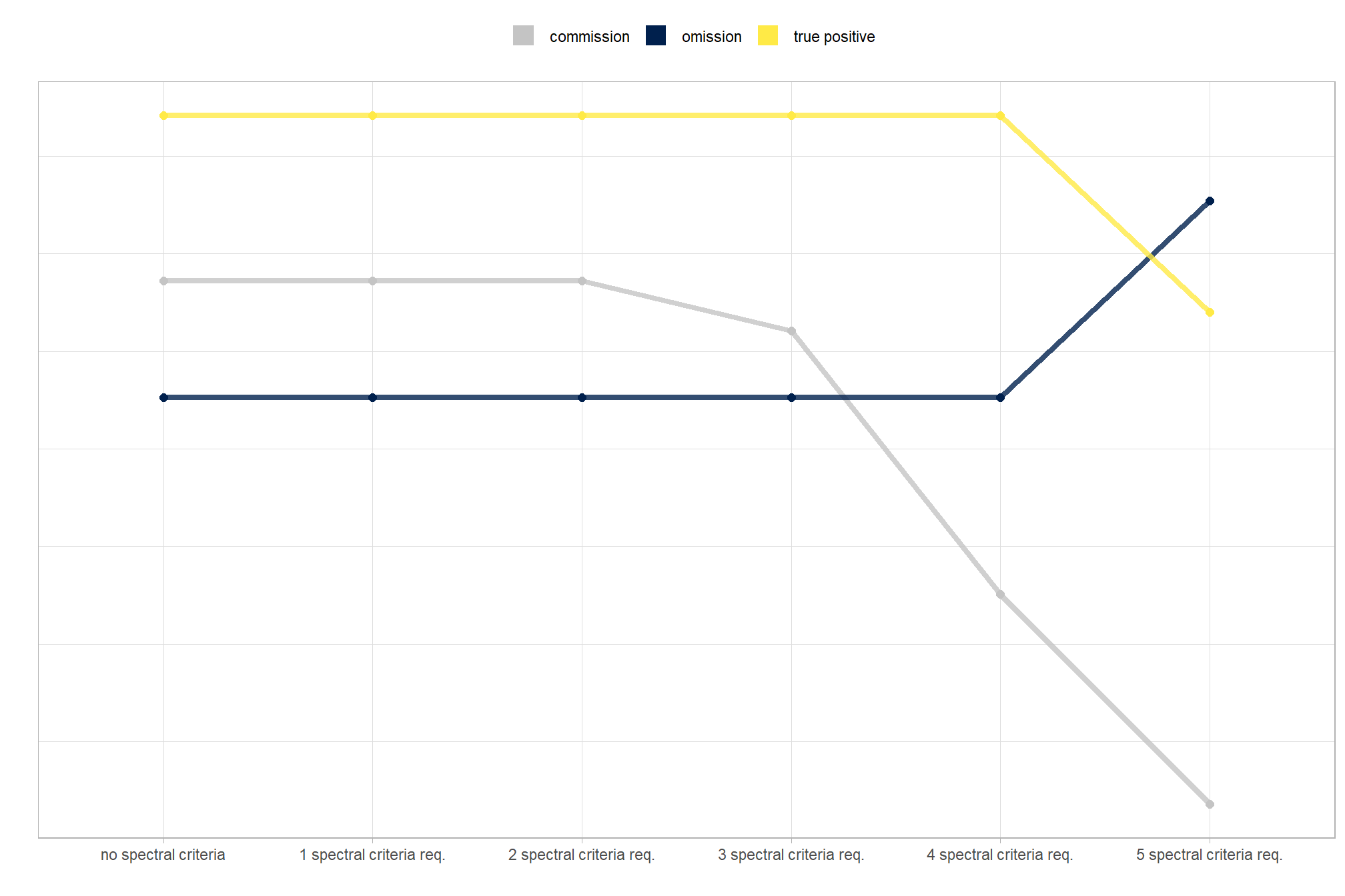
the trends here are as expected. however, for this data it appears that two criteria are highly correlated since we don’t see a change in the prediction classification until we require that at least three spectral index threshold criteria are met.
let’s look at a single parameter combination and the difference between different levels of spectral filtering
# plot it
ortho_plt_temp <- ortho_plt_fn(
    stand = stand_boundary %>%
      sf::st_transform(terra::crs(ortho_rast))
    , buffer = 30
  ) +
    ggplot2::geom_sf(
      data = stand_boundary %>%
        sf::st_transform(terra::crs(ortho_rast))
      , color = "black", fill = NA, lwd = 1.1
    )
# ortho_plt_temp
# filter for one combination

df_temp <- param_combos_spectral_gt %>%
  # dplyr::filter(rn == unique(param_combos_spectral_gt$rn) %>% sample(1))
  dplyr::filter(rn == 172)

# add piles
plt_list_temp <- c(0:5) %>%
  purrr::map(\(x)
    ortho_plt_temp +
      ggplot2::geom_sf(
        data =
          slash_piles_polys %>%
          dplyr::filter(is_in_stand) %>%
          sf::st_transform(terra::crs(ortho_rast)) %>%
            dplyr::left_join(
              df_temp %>%
                dplyr::filter(spectral_weight==x) %>%
                dplyr::select(pile_id,match_grp,spectral_weight_desc) %>%
                dplyr::mutate(pile_id=as.character(pile_id))
              , by = "pile_id"
            )
        , mapping = ggplot2::aes(color = match_grp)
        , inherit.aes = F
        , fill = NA , lwd = 0.7
      )+
      ggplot2::geom_sf(
        data =
          param_combos_piles %>%
            dplyr::inner_join(
              df_temp %>%
                dplyr::filter(is_in_stand & match_grp == "commission") %>%
                dplyr::filter(spectral_weight==x) %>%
                dplyr::select(pred_id,match_grp,spectral_weight_desc)
              , by = "pred_id"
            )
        , mapping = ggplot2::aes(color = match_grp)
        , inherit.aes = F
        , fill = NA , lwd = 0.4
      ) +
      ggplot2::scale_color_manual(
        values = c(
            "omission"= "blue2" # viridis::cividis(3)[1]
            , "commission"= "gray88" #viridis::cividis(3)[2]
            , "true positive"= "yellow2" #viridis::cividis(3)[3]
          )
        , name = ""
      ) +
      ggplot2::labs(
        subtitle = levels(param_combos_spectral_gt$spectral_weight_desc)[x+1]
      ) +
      ggplot2::theme(
        legend.position = "bottom"
        , plot.subtitle = ggplot2::element_text(size = 9, hjust = 0.4, face = "bold")
      ) +
      ggplot2::guides(
        color = ggplot2::guide_legend(override.aes = list(lwd = 9))
        , fill = "none"
      )
)patchwork::wrap_plots(
plt_list_temp
, ncol = 2
, guides = "collect"
) &
ggplot2::theme(legend.position = "bottom")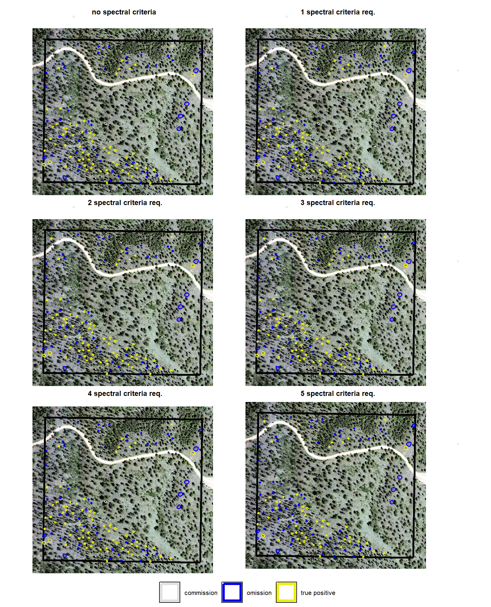
the spectral filtering performed as intended, successfully removing candidate piles that visually appear as green vegetation on the imagery and it also eliminated some candidates that appeared to be rocks or rock outcroppings, though with less success visually than for vegetation
8.2 Aggregate assessment metrics
now we need to aggregate the single-pile-level data into a single record for each parameter combination. aggregation will calculate detection performance metrics such as F-score, precision, and recall, as well as quantification accuracy metrics including Root Mean Squared Error (RMSE), Mean Error (ME), and Mean Absolute Percentage Error (MAPE) to assess the accuracy of our pile form measurements.
as a reminder regarding the form quantification accuracy evaluation, we will assess the method’s accuracy by comparing the true-positive matches using the following metrics:
- Volume compares the predicted volume from the irregular elevation profile and footprint to the ground truth paraboloid volume
- Diameter compares the predicted diameter (from the maximum internal distance) to the ground truth field-measured diameter.
- Area compares the predicted area from the irregular shape to the ground truth assumed circular area
- Height compares the predicted maximum height from the CHM to the ground truth field-measured height
# unique combinations
# param_combos_spectral_gt %>% dplyr::glimpse()
combo_temp <- param_combos_spectral_gt %>% dplyr::distinct(rn,spectral_weight)
# aggregate over combinations
param_combos_spectral_gt_agg <-
  1:nrow(combo_temp) %>%
  # 1:3 %>%
  purrr::map(
    \(x)
    agg_ground_truth_match(
      param_combos_spectral_gt %>%
        dplyr::filter(
          is_in_stand
          & rn == combo_temp$rn[x]
          & spectral_weight == combo_temp$spectral_weight[x]
        )
    ) %>%
    dplyr::mutate(
      rn = combo_temp$rn[x]
      , spectral_weight = combo_temp$spectral_weight[x]
    )
  ) %>%
  dplyr::bind_rows() %>%
  # add in info on all parameter combinations
  dplyr::inner_join(
    param_combos_df
    , by = "rn"
    , relationship = "many-to-one"
  )
# param_combos_spectral_gt %>%  dplyr::glimpse()
# param_combos_spectral_gt_agg %>% dplyr::glimpse()
# we can also add the relative rmse (rrmse) by comparing the rmse to the mean value of the ground truth data
param_combos_spectral_gt_agg <- param_combos_spectral_gt_agg %>%
  dplyr::bind_cols(
    # add means of gt
    slash_piles_polys %>%
      sf::st_drop_geometry() %>%
      dplyr::select(image_gt_area_m2,field_gt_area_m2,image_gt_volume_m3,field_gt_volume_m3,height_m,field_diameter_m) %>%
      dplyr::ungroup() %>%
      dplyr::summarise(dplyr::across(dplyr::everything(), ~mean(.x,na.rm=T))) %>%
      dplyr::rename_with(~ paste0("gt_", .x, recycle0 = TRUE))
  ) %>%
  dplyr::mutate(
    area_diff_field_rrmse = area_diff_field_rmse/gt_field_gt_area_m2
    # , area_diff_image_rrmse = area_diff_image_rmse/gt_image_gt_area_m2
    , volume_diff_field_rrmse = volume_diff_field_rmse/gt_field_gt_volume_m3
    # , volume_diff_image_rrmse = volume_diff_image_rmse/gt_image_gt_volume_m3
    # , paraboloid_volume_diff_field_rrmse = paraboloid_volume_diff_field_rmse/gt_field_gt_volume_m3
    # , paraboloid_volume_diff_image_rrmse = paraboloid_volume_diff_image_rmse/gt_image_gt_volume_m3
    , height_diff_rrmse = height_diff_rmse/gt_height_m
    , diameter_diff_rrmse = diameter_diff_rmse/gt_field_diameter_m
  ) %>%
  dplyr::select(!tidyselect::starts_with("gt_"))
# what is this?
param_combos_spectral_gt_agg %>% dplyr::glimpse()
## Rows: 8,640
## Columns: 31
## $ tp_n <dbl> 79, 73, 65, 54, 32, 4, 79, 73, 65, 54, 32, …
## $ fp_n <dbl> 44, 32, 17, 9, 0, 0, 44, 32, 17, 9, 0, 0, 4…
## $ fn_n <dbl> 42, 48, 56, 67, 89, 117, 42, 48, 56, 67, 89…
## $ omission_rate <dbl> 0.3471074, 0.3966942, 0.4628099, 0.5537190,…
## $ commission_rate <dbl> 0.3577236, 0.3047619, 0.2073171, 0.1428571,…
## $ precision <dbl> 0.6422764, 0.6952381, 0.7926829, 0.8571429,…
## $ recall <dbl> 0.65289256, 0.60330579, 0.53719008, 0.44628…
## $ f_score <dbl> 0.6475410, 0.6460177, 0.6403941, 0.5869565,…
## $ area_diff_field_rmse <dbl> 1.611770, 1.664736, 1.626639, 1.638681, 1.6…
## $ diameter_diff_rmse <dbl> 0.7485177, 0.7525893, 0.7488925, 0.7384185,…
## $ height_diff_rmse <dbl> 0.3094341, 0.3178506, 0.3062417, 0.3100133,…
## $ volume_diff_field_rmse <dbl> 2.134892, 2.206145, 2.192266, 2.191718, 2.0…
## $ area_diff_field_mean <dbl> 0.022080324, 0.021422253, -0.002900846, -0.…
## $ diameter_diff_mean <dbl> 0.6528961, 0.6522134, 0.6509824, 0.6366149,…
## $ height_diff_mean <dbl> -0.2040260, -0.2230022, -0.2209795, -0.2303…
## $ volume_diff_field_mean <dbl> -0.8267348, -0.8985110, -0.8974220, -0.8900…
## $ pct_diff_area_field_mape <dbl> 0.1775634, 0.1861107, 0.1824384, 0.1827844,…
## $ pct_diff_diameter_mape <dbl> 0.2236866, 0.2242669, 0.2226649, 0.2205699,…
## $ pct_diff_height_mape <dbl> 0.1295703, 0.1335366, 0.1332140, 0.1357417,…
## $ pct_diff_volume_field_mape <dbl> 0.2357586, 0.2456211, 0.2479493, 0.2558522,…
## $ rn <dbl> 1, 2, 3, 4, 5, 6, 7, 8, 9, 10, 11, 12, 13, …
## $ spectral_weight <dbl> 1, 1, 1, 1, 1, 1, 1, 1, 1, 1, 1, 1, 1, 1, 1…
## $ max_ht_m <dbl> 2, 2, 2, 2, 2, 2, 2, 2, 2, 2, 2, 2, 2, 2, 2…
## $ min_area_m2 <dbl> 2, 2, 2, 2, 2, 2, 2, 2, 2, 2, 2, 2, 2, 2, 2…
## $ max_area_m2 <dbl> 10, 10, 10, 10, 10, 10, 10, 10, 10, 10, 10,…
## $ convexity_pct <dbl> 0.3, 0.3, 0.3, 0.3, 0.3, 0.3, 0.4, 0.4, 0.4…
## $ circle_fit_iou_pct <dbl> 0.3, 0.4, 0.5, 0.6, 0.7, 0.8, 0.3, 0.4, 0.5…
## $ area_diff_field_rrmse <dbl> 0.1519422, 0.1569353, 0.1533438, 0.1544791,…
## $ volume_diff_field_rrmse <dbl> 0.1396832, 0.1443452, 0.1434371, 0.1434012,…
## $ height_diff_rrmse <dbl> 0.1417985, 0.1456554, 0.1403356, 0.1420639,…
## $ diameter_diff_rrmse <dbl> 0.2162193, 0.2173954, 0.2163276, 0.2133020,…# param_combos_spectral_gt_agg %>%
# dplyr::count(max_ht_m)
# param_combos_spectral_gt_agg %>%
# dplyr::distinct(
# max_ht_m, min_area_m2, max_area_m2, convexity_pct, circle_fit_iou_pct, spectral_weight
# ) %>%
# dplyr::count(max_ht_m) %>%
# dplyr::mutate(n2 = n/length(unique(param_combos_spectral_gt_agg$spectral_weight)))
# param_combos_df %>%
# dplyr::count(max_ht_m)8.3 Parameter Sensitivity Test Results
let’s get a quick summary of the evaluation metrics across all parameter combinations
# pal
pal_eval_metric <- c(
  RColorBrewer::brewer.pal(3,"Oranges")[3]
  , RColorBrewer::brewer.pal(3,"Greys")[3]
  , RColorBrewer::brewer.pal(3,"Purples")[3]
)
# summary
param_combos_spectral_gt_agg %>%
  dplyr::select(f_score,recall,precision,tidyselect::ends_with("_mape")) %>%
  summary()
## f_score recall precision pct_diff_area_field_mape
## Min. :0.0640 Min. :0.03306 Min. :0.2905 Min. :0.1062
## 1st Qu.:0.5062 1st Qu.:0.42975 1st Qu.:0.5894 1st Qu.:0.2187
## Median :0.6196 Median :0.65289 Median :0.7171 Median :0.2270
## Mean :0.5604 Mean :0.57943 Mean :0.7119 Mean :0.2220
## 3rd Qu.:0.7070 3rd Qu.:0.81818 3rd Qu.:0.8630 3rd Qu.:0.2346
## Max. :0.8193 Max. :0.91736 Max. :1.0000 Max. :0.2601
## pct_diff_diameter_mape pct_diff_height_mape pct_diff_volume_field_mape
## Min. :0.1343 Min. :0.09824 Min. :0.1032
## 1st Qu.:0.2377 1st Qu.:0.14032 1st Qu.:0.2825
## Median :0.2488 Median :0.17649 Median :0.2962
## Mean :0.2431 Mean :0.16909 Mean :0.2913
## 3rd Qu.:0.2557 3rd Qu.:0.19155 3rd Qu.:0.3150
## Max. :0.3053 Max. :0.20849 Max. :0.34338.3.1 Main effect of spectral data: pile detection
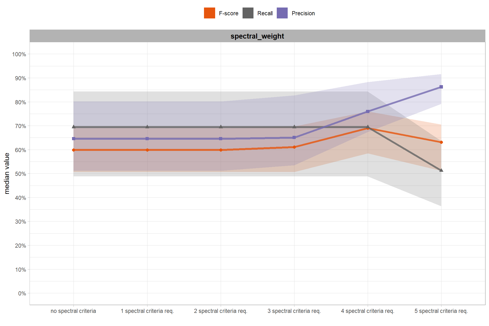
let’s average across all other factors to look at the main effect of spectral_weight which controls the strictness of our spectral filtering. as the spectral_weight parameter increases from its lowest setting (“1”, requiring only one spectral index threshold to be met) to its highest (“5”, requiring all spectral index thresholds be met)
param_combos_spectral_gt_agg %>%
  dplyr::select(c(spectral_weight,precision,recall,f_score)) %>%
  tidyr::pivot_longer(
    cols = c(precision,recall,f_score)
    , names_to = "metric"
    , values_to = "value"
  ) %>%
  tidyr::pivot_longer(
    cols = c(spectral_weight)
    , names_to = "param"
    , values_to = "param_value"
  ) %>%
  dplyr::group_by(param, param_value, metric) %>%
  dplyr::summarise(
    median = median(value,na.rm=T)
    , q25 = stats::quantile(value,na.rm=T,probs = 0.25)
    , q75 = stats::quantile(value,na.rm=T,probs = 0.75)
  ) %>%
  dplyr::ungroup() %>%
  dplyr::mutate(
    metric = dplyr::case_when(
        metric == "f_score" ~ 1
        , metric == "recall" ~ 2
        , metric == "precision" ~ 3
      ) %>%
      factor(
        ordered = T
        , levels = 1:3
        , labels = c(
          "F-score"
          , "Recall"
          , "Precision"
        )
      )
    , param_value = factor(x = param_value, labels = levels(param_combos_spectral_gt$spectral_weight_desc))
  ) %>%
  ggplot2::ggplot(
    mapping = ggplot2::aes(y = median, x = param_value, color = metric, fill = metric, group = metric, shape = metric)
  ) +
  ggplot2::geom_ribbon(
    mapping = ggplot2::aes(ymin = q25, ymax = q75)
    , alpha = 0.2, color = NA
  ) +
  ggplot2::geom_line(lwd = 1.5, alpha = 0.8) +
  ggplot2::geom_point(size = 2) +
  ggplot2::facet_wrap(facets = dplyr::vars(param), scales = "free_x") +
  # ggplot2::scale_color_viridis_d(begin = 0.2, end = 0.8) +
  ggplot2::scale_fill_manual(values = pal_eval_metric) +
  ggplot2::scale_color_manual(values = pal_eval_metric) +
  ggplot2::scale_y_continuous(limits = c(0,1), labels = scales::percent, breaks = scales::breaks_extended(10)) +
  ggplot2::labs(x = "", y = "median value", color = "", fill = "") +
  ggplot2::theme_light() +
  ggplot2::theme(
    legend.position = "top"
    , strip.text = ggplot2::element_text(size = 11, color = "black", face = "bold")
  ) +
  ggplot2::guides(
    color = ggplot2::guide_legend(override.aes = list(shape = 15, linetype = 0, size = 5, alpha = 1))
    , shape = "none"
  )
based on these main effect aggregated results:
- increasing the
spectral_weight(where “5” requires all spectral index thresholds to be met) had minimal impact on metrics until a value of “3”, at which point F-score and precision both saw slight improvements. at aspectral_weightof “4”, the F-score significantly improved due to a substantial increase in precision. settingspectral_weightto “5” resulted in a significant drop in recall (detection rate) and a proportionally inverse increase in precision, leading to only a minor overall change in F-score.
8.3.2 Main effect of spectral data: form quantification
let’s average across all other factors to look at the main effect by parameter for the MAPE metrics quantifying the pile form accuracy
param_combos_spectral_gt_agg %>%
  dplyr::select(
    spectral_weight
    , tidyselect::ends_with("_mape")
  ) %>%
  tidyr::pivot_longer(
    cols = c(tidyselect::ends_with("_mape"))
    , names_to = "metric"
    , values_to = "value"
  ) %>%
  tidyr::pivot_longer(
    cols = c(spectral_weight)
    , names_to = "param"
    , values_to = "param_value"
  ) %>%
  dplyr::group_by(param, param_value, metric) %>%
  dplyr::summarise(
    median = median(value,na.rm=T)
    , q25 = stats::quantile(value,na.rm=T,probs = 0.25)
    , q75 = stats::quantile(value,na.rm=T,probs = 0.75)
  ) %>%
  dplyr::ungroup() %>%
  dplyr::mutate(
    metric = dplyr::case_when(
        metric == "f_score" ~ 1
        , metric == "recall" ~ 2
        , metric == "precision" ~ 3
        # rmse
        , metric == "pct_diff_volume_field_mape" ~ 4
        , metric == "pct_diff_paraboloid_volume_field_mape" ~ 5
        , metric == "pct_diff_area_field_mape" ~ 6
        , metric == "pct_diff_height_mape" ~ 7
        , metric == "pct_diff_diameter_mape" ~ 8
      ) %>%
      factor(
        ordered = T
        , levels = 1:8
        , labels = c(
          "F-score"
          , "Recall"
          , "Precision"
          , "MAPE: Volume irregular (%)"
          , "MAPE: Volume paraboloid (%)"
          , "MAPE: Area (%)"
          , "MAPE: Height (%)"
          , "MAPE: Diameter (%)"
        )
      )
    , param_value = factor(x = param_value, labels = levels(param_combos_spectral_gt$spectral_weight_desc))
  ) %>%
  ggplot2::ggplot(
    mapping = ggplot2::aes(y = median, x = param_value, color = metric, fill = metric, group = metric, shape = metric)
  ) +
  # ggplot2::geom_ribbon(
  #   mapping = ggplot2::aes(ymin = q25, ymax = q75)
  #   , alpha = 0.2, color = NA
  # ) +
  ggplot2::geom_line(lwd = 1.5, alpha = 0.8) +
  ggplot2::geom_point(size = 2) +
  ggplot2::facet_wrap(facets = dplyr::vars(param), scales = "free_x") +
  ggplot2::scale_fill_viridis_d(option = "turbo") +
  ggplot2::scale_color_viridis_d(option = "turbo") +
  ggplot2::scale_shape_manual(values = c(15,16,17,18,0)) +
  ggplot2::scale_y_continuous(limits = c(0,1), labels = scales::percent, breaks = scales::breaks_extended(10)) +
  ggplot2::labs(x = "", y = "median value", color = "", fill = "") +
  ggplot2::theme_light() +
  ggplot2::theme(
    legend.position = "top"
    , strip.text = ggplot2::element_text(size = 11, color = "black", face = "bold")
  ) +
  ggplot2::guides(
    color = ggplot2::guide_legend(override.aes = list(shape = 15, linetype = 0, size = 5, alpha = 1))
    , shape = "none"
  )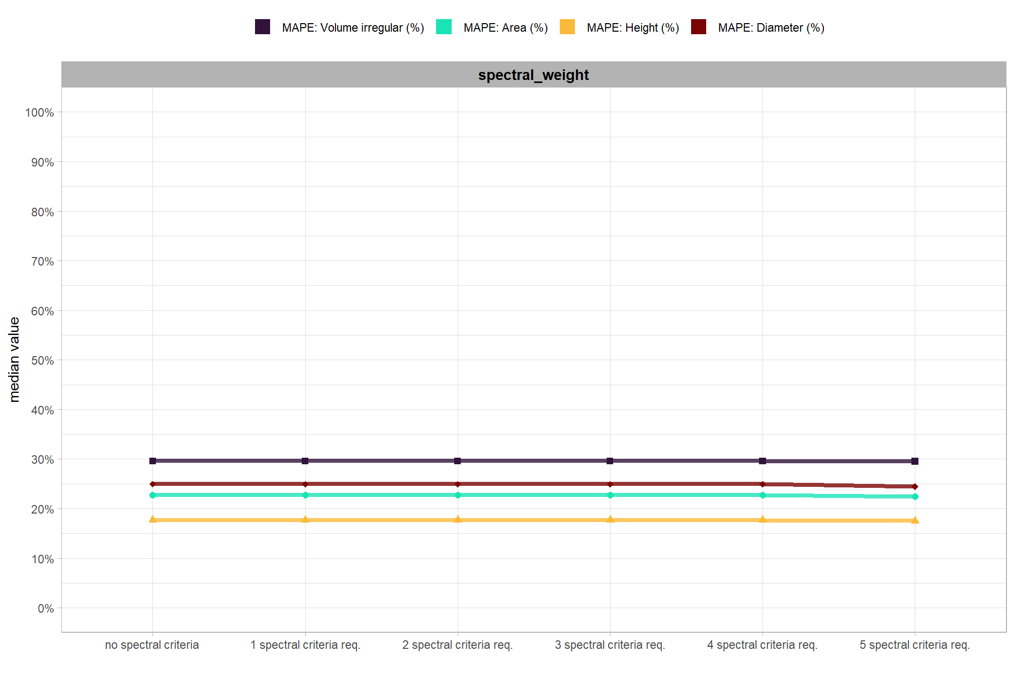
these results indicate that the method’s accuracy in outlining slash pile form is robust to parameter changes, as the relevant shape accuracy metrics remain consistent across various settings of the spectral_weight parameter
8.3.3 Overall: pile detection
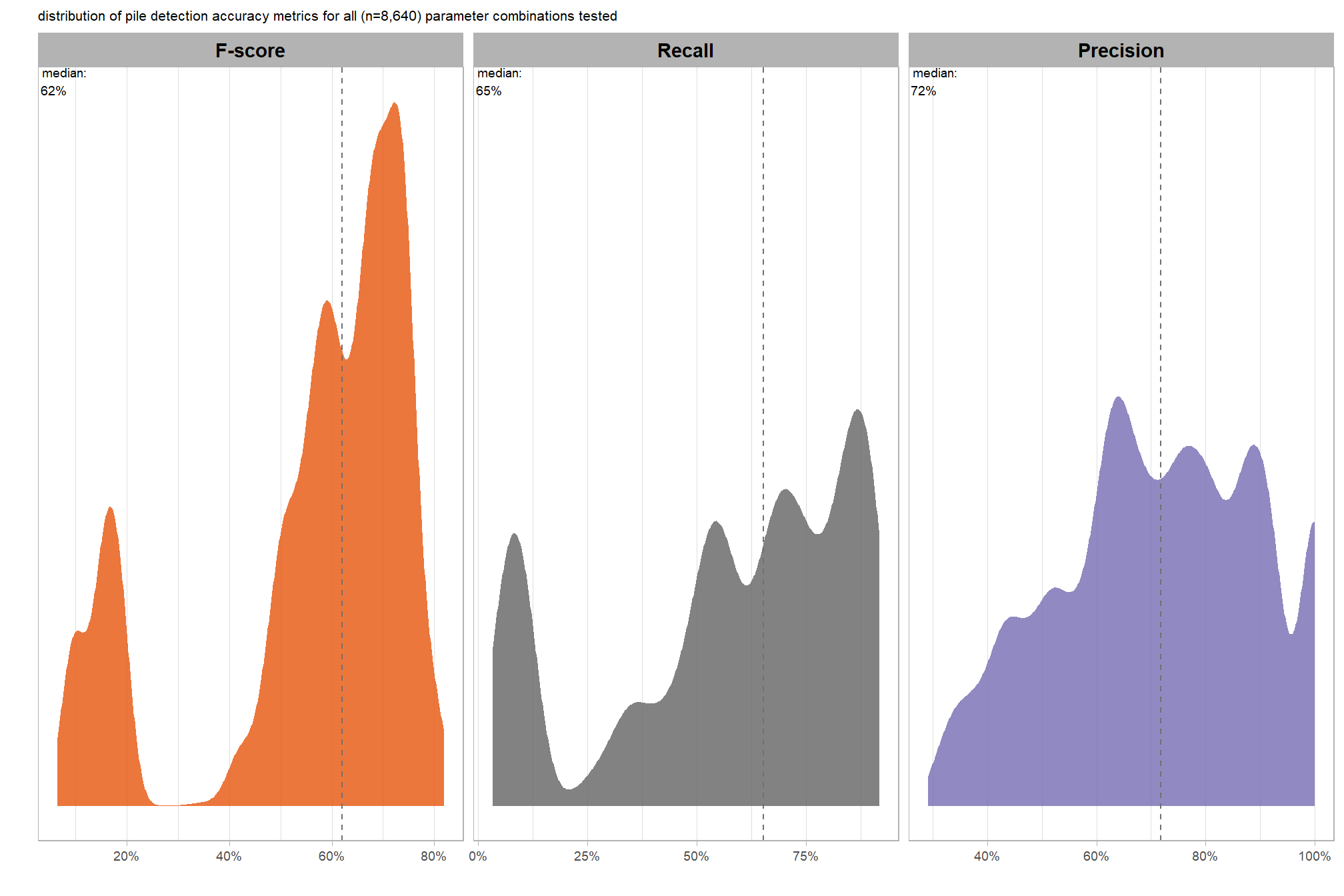
let’s check out the distribution of the instance segmentation (i.e. pile detection) results by looking at the detection accuracy metrics where:
- Precision precision measures how many of the objects our method detected as slash piles were actually correct. A high precision means the method has a low rate of false alarms.
- Recall recall (i.e. detection rate) indicates how many actual (ground truth) slash piles our method successfully identified. High recall means the method is good at finding most existing piles, minimizing omissions.
- F-score provides a single, balanced measure that combines both precision and recall. A high F-score indicates overall effectiveness in both finding most piles and ensuring most detections are correct.
# plot it
plt_detection_dist(
  df = param_combos_spectral_gt_agg
  , paste0(
     "distribution of pile detection accuracy metrics for all"
     , " (n="
     , scales::comma(nrow(param_combos_spectral_gt_agg), accuracy = 1)
     , ") "
     , "parameter combinations tested"
    )
  , show_rug = F
)
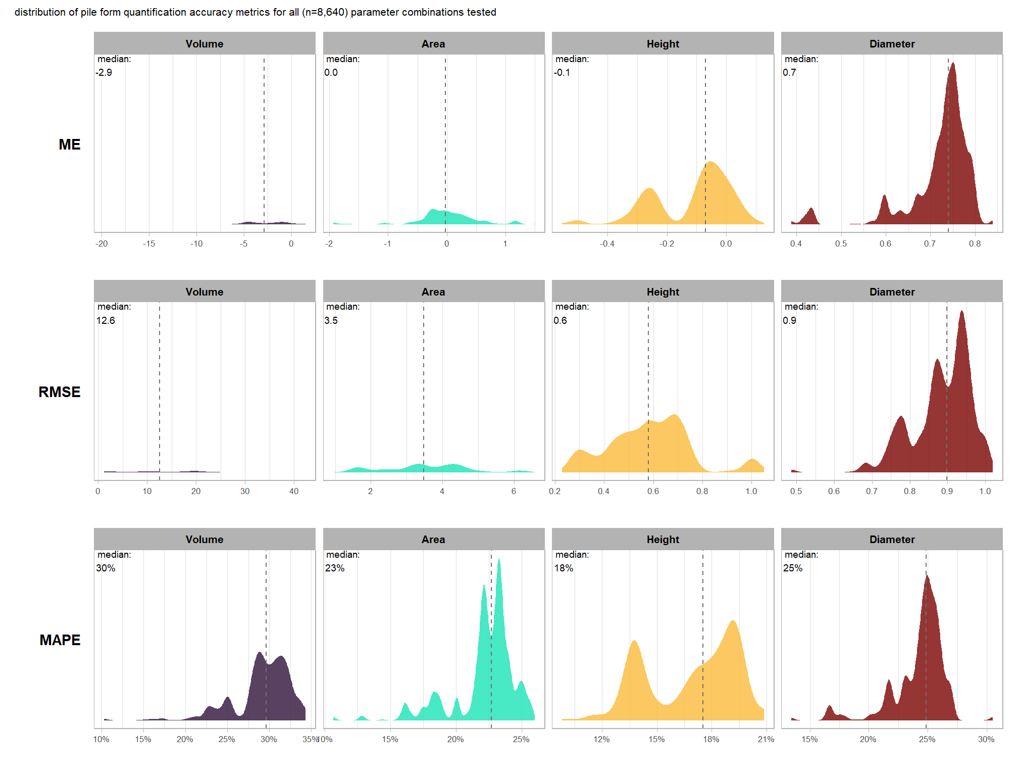
8.3.4 Overall: form quantification
let’s check out the the ability of the method to properly extract the form of the piles by looking at the quantification accuracy metrics where:
- Mean Error (ME) represents the direction of bias (over or under-prediction) in the original units
- RMSE represents the typical magnitude of error in the original units, with a stronger penalty for large errors
- MAPE represents the typical magnitude of error as a percentage, allowing for scale-independent comparisons
as a reminder regarding the form quantification accuracy evaluation, we will assess the method’s accuracy by comparing the true-positive matches using the following metrics:
- Volume compares the predicted volume from the irregular elevation profile and footprint to the ground truth paraboloid volume
- Diameter compares the predicted diameter (from the maximum internal distance) to the ground truth field-measured diameter.
- Area compares the predicted area from the irregular shape to the ground truth assumed circular area
- Height compares the predicted maximum height from the CHM to the ground truth field-measured height
# plot it
plt_form_quantification_dist(
  df = param_combos_spectral_gt_agg %>% dplyr::slice_sample(prop = 0.3)
  , paste0(
     "distribution of pile form quantification accuracy metrics for all"
     , " (n="
     , scales::comma(nrow(param_combos_spectral_gt_agg), accuracy = 1)
     , ") "
     , "parameter combinations tested"
  )
  , show_rug = F
)
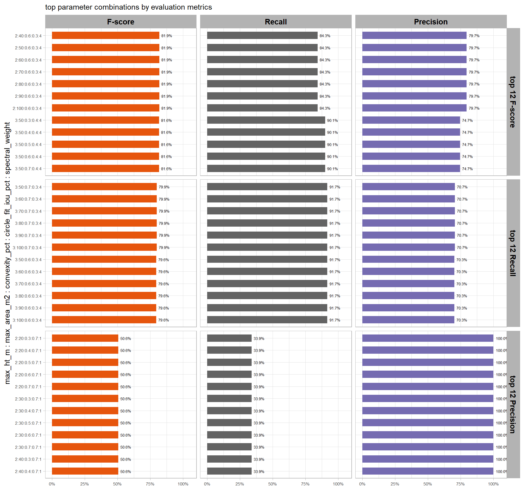
8.3.5 Best results: detection accuracy
we can cut to the chase and just look at the parameter combinations that achieved the best results based on the evaluation metrics
rank_th_temp <- 12
df_temp <-
  param_combos_spectral_gt_agg %>%
  dplyr::ungroup() %>%
  dplyr::arrange(desc(f_score)) %>%
  dplyr::mutate(
    rank_f_score = dplyr::row_number()
  ) %>%
  dplyr::arrange(desc(precision)) %>%
  dplyr::mutate(
    rank_precision = dplyr::row_number()
  ) %>%
  dplyr::arrange(desc(recall)) %>%
  dplyr::mutate(
    rank_recall = dplyr::row_number()
  ) %>%
  dplyr::arrange(desc(f_score), desc(recall), desc(precision)) %>%
  # now get the max of these pct ranks by row
  dplyr::rowwise() %>%
  dplyr::mutate(
    rank_min = min(
      dplyr::c_across(
        tidyselect::starts_with("rank")
      )
      , na.rm = T
    )
  ) %>%
  dplyr::ungroup() %>%
  dplyr::mutate(
    rank_lab = dplyr::case_when(
      rank_f_score<=rank_th_temp ~ 1
      , rank_recall<=rank_th_temp ~ 2
      , rank_precision<=rank_th_temp ~ 3
      , (rank_f_score>=(nrow(param_combos_spectral_gt_agg)-rank_th_temp) & dplyr::coalesce(f_score,0)>0) ~ 4
    ) %>%
      factor(
        ordered = T
        , levels = 1:4
        , labels = c(
          paste0("top ", scales::comma(rank_th_temp, accuracy = 1), " F-score")
          , paste0("top ", scales::comma(rank_th_temp, accuracy = 1), " Recall")
          , paste0("top ", scales::comma(rank_th_temp, accuracy = 1), " Precision")
          , paste0("bottom ", scales::comma(rank_th_temp, accuracy = 1), " F-score")
        )
      )
  ) %>%
  dplyr::filter(
    !is.na(rank_lab) # rank_min>=0.99
  ) %>%
  dplyr::mutate(
    lab = stringr::str_c(max_ht_m,max_area_m2,convexity_pct,circle_fit_iou_pct,spectral_weight, sep = ":")
  )
# plot
df_temp %>%
  dplyr::filter(!stringr::str_starts(rank_lab, "bottom")) %>%
  tidyr::pivot_longer(
    cols = c(precision,recall,f_score)
    , names_to = "metric"
    , values_to = "value"
  ) %>%
  dplyr::mutate(
    metric = dplyr::case_when(
        metric == "f_score" ~ 1
        , metric == "recall" ~ 2
        , metric == "precision" ~ 3
      ) %>%
      factor(
        ordered = T
        , levels = 1:3
        , labels = c(
          "F-score"
          , "Recall"
          , "Precision"
        )
      )
    , lab = forcats::fct_reorder(lab, desc(rank_f_score))
    , val_lab = scales::percent(value, accuracy = 0.1)
  ) %>%
  ggplot2::ggplot(
    mapping = ggplot2::aes(x = value, y = lab, fill = metric, label = val_lab)
  ) +
  ggplot2::geom_col(width = 0.6) +
  ggplot2::geom_text(color = "black", size = 2, hjust = -0.2) +
  ggplot2::scale_fill_manual(values = pal_eval_metric) +
  ggplot2::scale_x_continuous(
    labels = scales::percent_format(accuracy = 1)
    , limits = c(0,1.05)
    # , expand = expansion(mult = c(0, .08))
  ) +
  ggplot2::facet_grid(cols = dplyr::vars(metric), rows = dplyr::vars(rank_lab), scales = "free_y") +
  ggplot2::labs(
    x = "", y = "max_ht_m : max_area_m2 : convexity_pct : circle_fit_iou_pct : spectral_weight"
    , fill = ""
    , subtitle = "top parameter combinations by evaluation metrics"
  ) +
  ggplot2::theme_light() +
  ggplot2::theme(
    legend.position = "none"
    , strip.text = ggplot2::element_text(size = 11, color = "black", face = "bold")
    , axis.text = ggplot2::element_text(size = 6.2)
  )
let’s make a table of these results
df_temp %>%
  dplyr::filter(rank_min<=rank_th_temp) %>%
  dplyr::select(
    rank_lab
    , max_ht_m,max_area_m2,convexity_pct,circle_fit_iou_pct,spectral_weight
    , f_score, recall, precision
  ) %>%
  dplyr::ungroup() %>%
  dplyr::arrange(rank_lab,desc(f_score), desc(recall), desc(precision)) %>%
  dplyr::mutate(dplyr::across(
    .cols = c(f_score, recall, precision)
    , .fn = ~ scales::percent(.x, accuracy = 1)
  )) %>%
  dplyr::mutate(blank= "   " ) %>%
  dplyr::relocate(blank, .before = f_score) %>%
  kableExtra::kbl(
    caption = "parameter combinations that achieved the best slash pile detection results"
    , col.names = c(
      "."
      ,"max_ht_m","max_area_m2","convexity_pct","circle_fit_iou_pct","spectral_weight"
      , "   "
      , "F-score", "Recall", "Precision"
    )
    , escape = F
  ) %>%
  kableExtra::kable_styling(font_size = 10.5) %>%
  kableExtra::collapse_rows(columns = 1, valign = "top") %>%
kableExtra::add_header_above(c(" "=7, "Evaluation Metric" = 3))| . | max_ht_m | max_area_m2 | convexity_pct | circle_fit_iou_pct | spectral_weight | F-score | Recall | Precision | |
|---|---|---|---|---|---|---|---|---|---|
| top 12 F-score | 2 | 40 | 0.6 | 0.3 | 4 | 82% | 84% | 80% | |
| 2 | 50 | 0.6 | 0.3 | 4 | 82% | 84% | 80% | ||
| 2 | 60 | 0.6 | 0.3 | 4 | 82% | 84% | 80% | ||
| 2 | 70 | 0.6 | 0.3 | 4 | 82% | 84% | 80% | ||
| 2 | 80 | 0.6 | 0.3 | 4 | 82% | 84% | 80% | ||
| 2 | 90 | 0.6 | 0.3 | 4 | 82% | 84% | 80% | ||
| 2 | 100 | 0.6 | 0.3 | 4 | 82% | 84% | 80% | ||
| 3 | 50 | 0.3 | 0.4 | 4 | 82% | 90% | 75% | ||
| 3 | 50 | 0.4 | 0.4 | 4 | 82% | 90% | 75% | ||
| 3 | 50 | 0.5 | 0.4 | 4 | 82% | 90% | 75% | ||
| 3 | 50 | 0.6 | 0.4 | 4 | 82% | 90% | 75% | ||
| 3 | 50 | 0.7 | 0.4 | 4 | 82% | 90% | 75% | ||
| top 12 Recall | 3 | 50 | 0.7 | 0.3 | 4 | 80% | 92% | 71% | |
| 3 | 60 | 0.7 | 0.3 | 4 | 80% | 92% | 71% | ||
| 3 | 70 | 0.7 | 0.3 | 4 | 80% | 92% | 71% | ||
| 3 | 80 | 0.7 | 0.3 | 4 | 80% | 92% | 71% | ||
| 3 | 90 | 0.7 | 0.3 | 4 | 80% | 92% | 71% | ||
| 3 | 100 | 0.7 | 0.3 | 4 | 80% | 92% | 71% | ||
| 3 | 50 | 0.6 | 0.3 | 4 | 80% | 92% | 70% | ||
| 3 | 60 | 0.6 | 0.3 | 4 | 80% | 92% | 70% | ||
| 3 | 70 | 0.6 | 0.3 | 4 | 80% | 92% | 70% | ||
| 3 | 80 | 0.6 | 0.3 | 4 | 80% | 92% | 70% | ||
| 3 | 90 | 0.6 | 0.3 | 4 | 80% | 92% | 70% | ||
| 3 | 100 | 0.6 | 0.3 | 4 | 80% | 92% | 70% | ||
| top 12 Precision | 2 | 20 | 0.3 | 0.7 | 1 | 51% | 34% | 100% | |
| 2 | 20 | 0.4 | 0.7 | 1 | 51% | 34% | 100% | ||
| 2 | 20 | 0.5 | 0.7 | 1 | 51% | 34% | 100% | ||
| 2 | 20 | 0.6 | 0.7 | 1 | 51% | 34% | 100% | ||
| 2 | 20 | 0.7 | 0.7 | 1 | 51% | 34% | 100% | ||
| 2 | 30 | 0.3 | 0.7 | 1 | 51% | 34% | 100% | ||
| 2 | 30 | 0.4 | 0.7 | 1 | 51% | 34% | 100% | ||
| 2 | 30 | 0.5 | 0.7 | 1 | 51% | 34% | 100% | ||
| 2 | 30 | 0.6 | 0.7 | 1 | 51% | 34% | 100% | ||
| 2 | 30 | 0.7 | 0.7 | 1 | 51% | 34% | 100% | ||
| 2 | 40 | 0.3 | 0.7 | 1 | 51% | 34% | 100% | ||
| 2 | 40 | 0.4 | 0.7 | 1 | 51% | 34% | 100% |
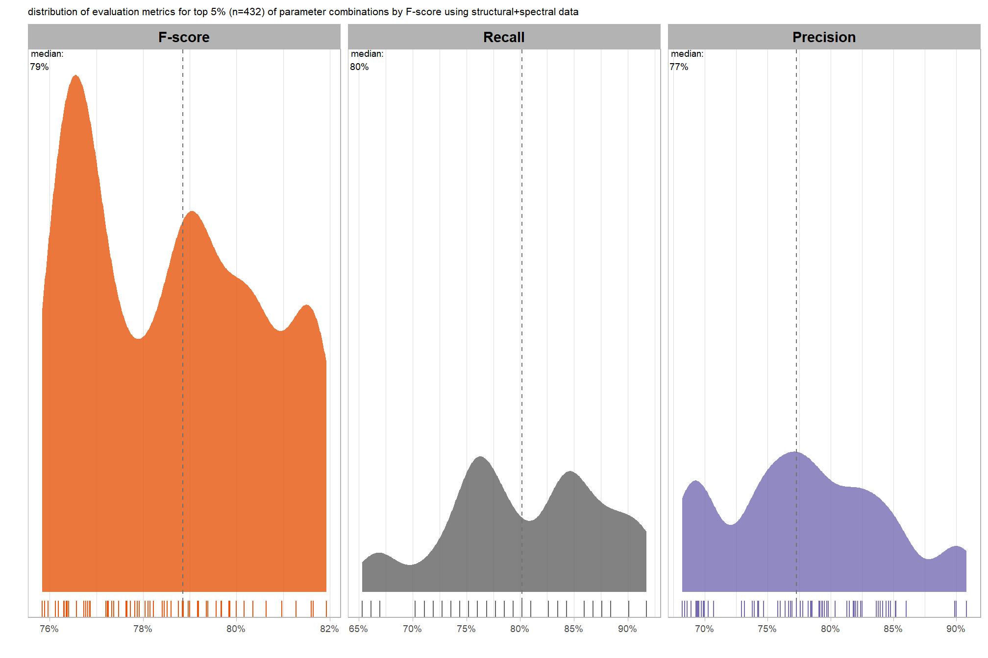
let’s look at only the top 5% of parameter combinations by F-score
# filter parameter combos for top x pct
top_x_pct_fscore <-
  param_combos_spectral_gt_agg %>%
    dplyr::ungroup() %>%
    dplyr::arrange(desc(f_score)) %>%
    dplyr::mutate(
      pct_rank_f_score = dplyr::percent_rank(f_score)
    ) %>%
    dplyr::filter(pct_rank_f_score>=pct_rank_th_top)
# plot it
plt_detection_dist(
  df = top_x_pct_fscore
  , paste0(
     "distribution of evaluation metrics for top "
     , scales::percent(1-pct_rank_th_top,accuracy=1)
     , " (n="
     , scales::comma(nrow(top_x_pct_fscore), accuracy = 1)
     , ") "
     , "of parameter combinations by F-score using structural+spectral data"
  )
)
if we look at only the top 5% of parameter combinations by F-score, what is the distribution of individual parameter settings?
pal_param <- viridis::plasma(n=5, begin = 0.1, end = 0.9, alpha = 0.8)
df_temp <- top_x_pct_fscore %>%
  dplyr::select(tidyselect::contains("f_score"), max_ht_m,max_area_m2,convexity_pct,circle_fit_iou_pct,spectral_weight) %>%
  tidyr::pivot_longer(
    cols = c(max_ht_m,max_area_m2,convexity_pct,circle_fit_iou_pct,spectral_weight)
    , names_to = "metric"
    , values_to = "value"
  ) %>%
  dplyr::count(metric, value) %>%
  dplyr::group_by(metric) %>%
  dplyr::mutate(
    pct=n/sum(n)
    , lab = paste0(scales::percent(pct,accuracy=0.1), "\nn=", scales::comma(n,accuracy=1))
  )
# save best for later
best_spectral_weight <- df_temp %>%
  dplyr::filter(metric=="spectral_weight") %>%
  dplyr::arrange(desc(n)) %>%
  dplyr::slice(1) %>%
  dplyr::pull(value)
# plot
df_temp %>%
  ggplot2::ggplot(
    mapping = ggplot2::aes(x = factor(value), y=pct, label=lab, fill = metric)
  ) +
  ggplot2::geom_col(width = 0.6) +
  ggplot2::geom_text(color = "black", size = 2.5, vjust = -0.2) +
  ggplot2::facet_wrap(facets = dplyr::vars(metric), ncol=2, scales = "free_x") +
  ggplot2::scale_y_continuous(
    breaks = seq(0,1,by=0.2)
    , labels = scales::percent
    , expand = ggplot2::expansion(mult = c(0,0.2))
  ) +
  ggplot2::scale_fill_manual(values = pal_param) +
  ggplot2::labs(
    x = "parameter setting", y = ""
    , fill = ""
    , subtitle = paste0(
       "parameter settings of top "
       , scales::percent(1-pct_rank_th_top,accuracy=1)
       , " (n="
       , scales::comma(nrow(top_x_pct_fscore), accuracy = 1)
       , ") "
       , "of parameter combinations by F-score using structural+spectral data"
    )
  ) +
  ggplot2::theme_light() +
  ggplot2::theme(
    legend.position = "none"
    , strip.text = ggplot2::element_text(size = 11, color = "black", face = "bold")
    , axis.text.y = ggplot2::element_text(size = 6)
    , axis.text.x = ggplot2::element_text(size = 8)
    , plot.subtitle = ggplot2::element_text(size = 8)
  )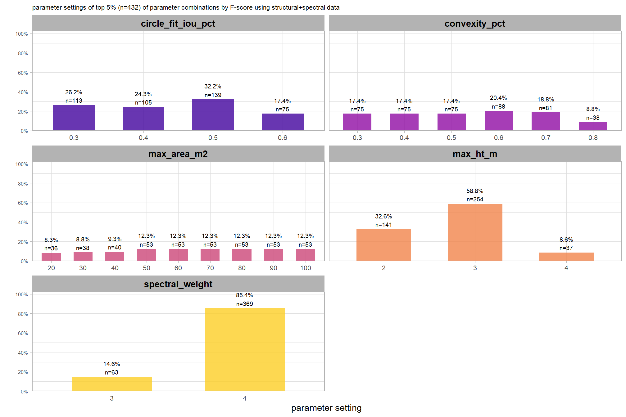
let’s use the value of spectral_weight that most frequently results in the best pile detection based on F-score (spectral_weight of “4”) to compare results to not using any spectral data (i.e. just using structural data as outlined in our method here). We’ll then average across all other factors to look at the main effect of spectral_weight after creating a dichotomous factor of structural only versus structural+spectral
# filter data
combos_df_temp <-
  param_combos_spectral_gt_agg %>%
  dplyr::mutate(
    combo = forcats::fct_cross(
      factor(max_ht_m)
      , factor(max_area_m2)
      , factor(convexity_pct)
      , factor(circle_fit_iou_pct)
    )
  ) %>%
  dplyr::select(c(
    combo,spectral_weight
    ,precision,recall,f_score
    , pct_diff_volume_field_mape, pct_diff_diameter_mape, pct_diff_area_field_mape, pct_diff_height_mape
  )) %>%
  dplyr::filter(
    spectral_weight == 0
    | spectral_weight == best_spectral_weight
  ) %>%
  dplyr::mutate(
    spectral_weight_fact = ifelse(spectral_weight==0,"structural only","structural+spectral") %>%
      factor()
  )

# quick mod
dep_vars_temp <- c("f_score","recall","precision")
# list of formulas
formulas_temp <- dep_vars_temp %>%
  purrr::map(~stats::reformulate(c("spectral_weight_fact","-1"), response = .x))
names(formulas_temp) <- dep_vars_temp
# formulas_temp
models_temp <- formulas_temp %>%
  purrr::map(\(x) lm(formula = x, data = combos_df_temp))
names(models_temp) <- dep_vars_temp
# models_temp
# combine into df
pred_df_temp <- purrr::map_df(models_temp, broom::tidy, .id = "metric") %>%
  dplyr::select(-c(statistic)) %>%
  dplyr::mutate(
    dep_var = dplyr::case_when(
        metric == "f_score" ~ 1
        , metric == "recall" ~ 2
        , metric == "precision" ~ 3
      ) %>%
      factor(
        ordered = T
        , levels = 1:3
        , labels = c(
          "F-score"
          , "Recall"
          , "Precision"
        )
      )
    , term = stringr::str_remove_all(term, "spectral_weight_fact") %>% factor()
    # to obtain the 95% confidence interval...
      # ...1.96 times the standard error is added and subtracted from the sample mean
    , ul = estimate+std.error*1.96
    , ll = estimate-std.error*1.96
  ) %>%
  dplyr::rename(spectral_weight_fact=term) %>%
  dplyr::relocate(dep_var) %>%
  dplyr::arrange(dep_var,spectral_weight_fact)

# pred_df_temp
# table it
pred_df_temp %>%
  dplyr::select(-c(metric,ul,ll)) %>%
  dplyr::mutate(
    estimate = scales::percent(estimate, accuracy = 0.1)
    , std.error = scales::percent(std.error, accuracy = 0.01)
    , p.value = ifelse(
        p.value < 0.001
        , "< 0.001"
        , scales::comma(p.value, accuracy = 0.0001)
      )
  ) %>%
  kableExtra::kbl(
    caption = "Predictions for detection accuracy metrics by detection method<br>averaging across all other structural detection parameters"
    , col.names = c(".","method","predicted mean", "SE", "p-value")
  ) %>%
  kableExtra::kable_styling() %>%
kableExtra::collapse_rows(columns = 1, valign = "top")| . | method | predicted mean | SE | p-value |
|---|---|---|---|---|
| F-score | structural only | 54.7% | 0.55% | < 0.001 |
| structural+spectral | 60.8% | 0.55% | < 0.001 | |
| Recall | structural only | 60.3% | 0.73% | < 0.001 |
| structural+spectral | 60.3% | 0.73% | < 0.001 | |
| Precision | structural only | 65.7% | 0.43% | < 0.001 |
| structural+spectral | 76.5% | 0.43% | < 0.001 |
plot the change from including spectral data to the pile detection methodology
# scales::show_col(pal_eval_metric)
# plot
ggplot2::ggplot(
  data = pred_df_temp
  , mapping = ggplot2::aes(x = spectral_weight_fact)
) +
  ggplot2::geom_line(
    data = combos_df_temp %>%
      dplyr::slice_sample(prop = 0.44) %>%
      tidyr::pivot_longer(
        cols = c(precision,recall,f_score)
        , names_to = "metric"
        , values_to = "value"
      ) %>%
      dplyr::mutate(
        dep_var = dplyr::case_when(
          metric == "f_score" ~ 1
          , metric == "recall" ~ 2
          , metric == "precision" ~ 3
        ) %>%
        factor(
          ordered = T
          , levels = 1:3
          , labels = c(
            "F-score"
            , "Recall"
            , "Precision"
          )
        )
      )
    , mapping = ggplot2::aes(y = value, group = combo, color = metric)
    , lwd = 0.6, alpha = 0.1
    # , color = pal_eval_metric[1]
  ) +
  geom_ribbon(
    mapping = ggplot2::aes(ymin = ll, ymax = ul, group = 1)
    , fill = "black", alpha = 0.2
  ) +
  ggplot2::geom_line(
    mapping = ggplot2::aes(y = estimate, group = 1)
    , lwd = 1, color = "black" # pal_eval_metric[1]
  ) +
  ggplot2::geom_text(
    mapping = ggplot2::aes(y=estimate, label = scales::percent(estimate,accuracy=0.1), group = 1)
    , vjust = -0.25
  ) +
  ggplot2::facet_wrap(facets = dplyr::vars(dep_var)) +
  ggplot2::scale_color_manual(values = c(pal_eval_metric[1],pal_eval_metric[3],pal_eval_metric[2]) ) + # pal_eval_metric
  ggplot2::scale_y_continuous(limits = c(0,1), labels = scales::percent, breaks = scales::breaks_extended(10)) +
  ggplot2::labs(
    x = "", y = "", color = "", fill = ""
    , caption = paste0(
      "*The spectral+structural group has the `spectral_weight` parameter set to '"
      , best_spectral_weight, "'"
    )
  ) +
  ggplot2::theme_light() +
  ggplot2::theme(
    legend.position = "none"
    , strip.text = ggplot2::element_text(size = 11, color = "black", face = "bold")
    , plot.caption = ggplot2::element_text(size = 8)
  )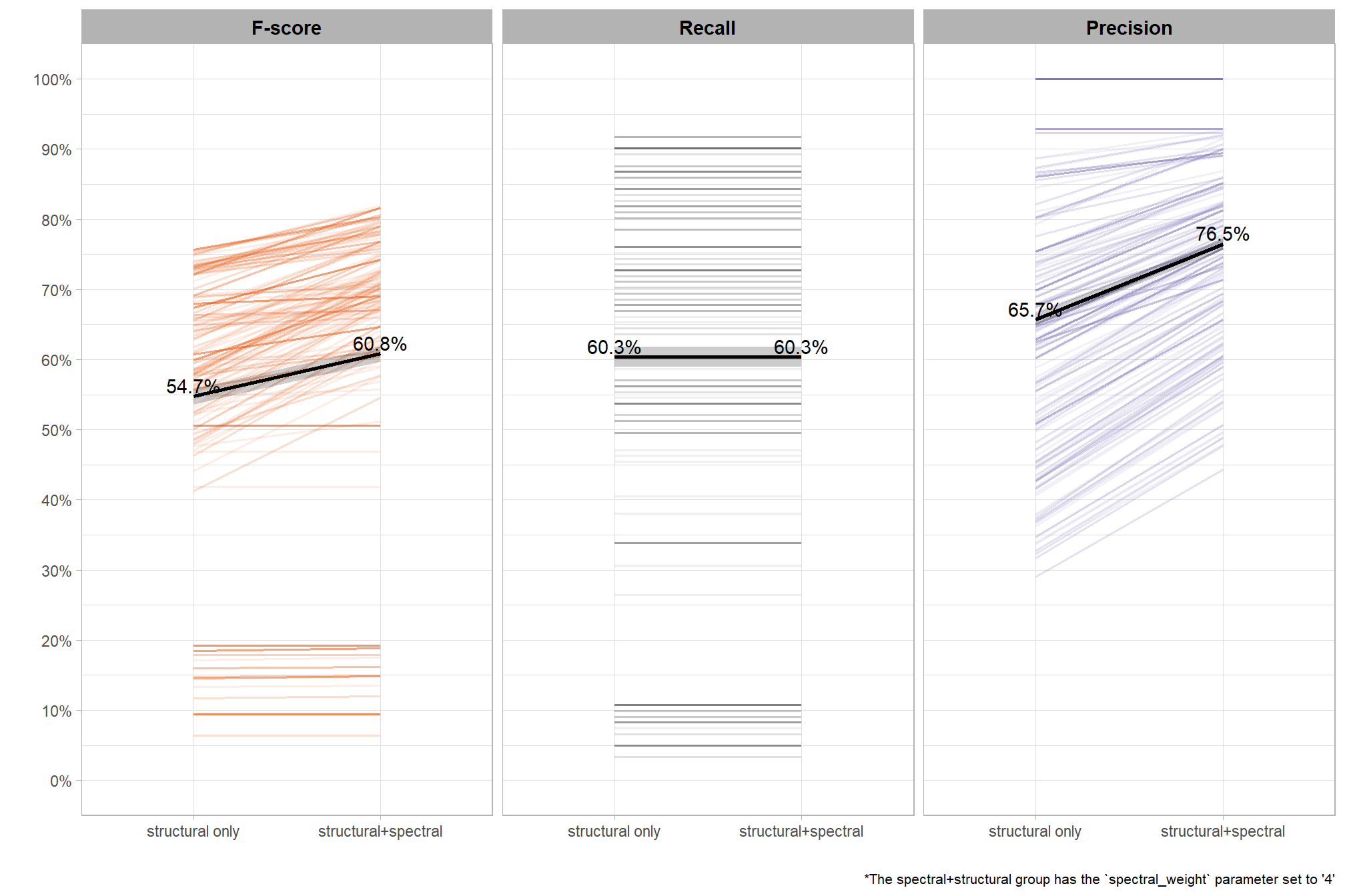
remember, these values appear low but the value is not the important takeaway here because we averaged across all other parameter settings, including those that resulted in poor pile detection, instead the focus is on the change from including the spectral data. based on the data used here, these results indicate that including the spectral data resulted in a 6.1 percentage point increase in the F-score compared to just using the structural data irrespective of the parameter settings used in the structural detection method.
if we look at only the best pile detection methodology based on F-score using the structural data and the best using both structural and spectral data, what is the change in our performance metrics from including the spectral data?
df_temp <-
  combos_df_temp %>%
  # get the top by spectral_weight
  dplyr::group_by(spectral_weight) %>%
  dplyr::mutate(
    is_top = f_score == max(f_score)
    , top_what = ifelse(is_top, spectral_weight, NA)
  ) %>%
  dplyr::arrange(desc(f_score),desc(recall),pct_diff_volume_field_mape,pct_diff_area_field_mape,pct_diff_height_mape) %>%
  dplyr::filter(dplyr::row_number() == 1) %>%
  dplyr::ungroup()

  # add top

combos_df_temp <-
  df_temp %>%
    dplyr::bind_rows(
      combos_df_temp %>%
      dplyr::filter(spectral_weight!=0) %>%
      dplyr::inner_join(
        df_temp %>% dplyr::filter(spectral_weight==0 & is_top) %>% dplyr::select(combo)
      ) %>%
      dplyr::mutate(
        is_top = F
        , top_what = 0
      )
    ) %>%
    dplyr::bind_rows(
      combos_df_temp %>%
      dplyr::filter(spectral_weight==0) %>%
      dplyr::inner_join(
        df_temp %>% dplyr::filter(spectral_weight!=0 & is_top) %>% dplyr::select(combo)
      ) %>%
      dplyr::mutate(
        is_top = F
        , top_what = max(df_temp$spectral_weight)
      )
    ) %>%
  dplyr::ungroup() %>%
  dplyr::mutate(
    top_what = ifelse(top_what==0,"Top structural only","Top structural+spectral") %>%
      factor()
    , desc = paste0(
      top_what
      , " : max_ht_m=", stringr::word(combo,1,sep = ":")
      , ", max_area_m2=", stringr::word(combo,2,sep = ":")
      , ", convexity_pct=", stringr::word(combo,3,sep = ":")
      , ", circle_fit_iou_pct=", stringr::word(combo,4,sep = ":")
    )
  )
# plot
combos_df_temp %>%
  tidyr::pivot_longer(
    cols = c(precision,recall,f_score)
    , names_to = "metric"
    , values_to = "value"
  ) %>%
  dplyr::mutate(
    dep_var = dplyr::case_when(
      metric == "f_score" ~ 1
      , metric == "recall" ~ 2
      , metric == "precision" ~ 3
    ) %>%
    factor(
      ordered = T
      , levels = 1:3
      , labels = c(
        "F-score"
        , "Recall"
        , "Precision"
      )
    )
  ) %>%
# plot
ggplot2::ggplot(
  mapping = ggplot2::aes(x = spectral_weight_fact,y = value,label = scales::percent(value,accuracy=0.1), group = combo, color = desc)
) +
  ggplot2::geom_line(key_glyph = "point") +
  ggplot2::geom_text(
    vjust = -0.25
    , show.legend = FALSE
  ) +
  ggplot2::facet_wrap(facets = dplyr::vars(dep_var)) +
  harrypotter::scale_color_hp_d(option = "hermionegranger") +
  ggplot2::scale_y_continuous(limits = c(0,1), labels = scales::percent, breaks = scales::breaks_extended(10)) +
  ggplot2::labs(
    x = "", y = "", color = "", fill = ""
    , caption = paste0(
      "*The spectral+structural group has the `spectral_weight` parameter set to '"
      , best_spectral_weight, "'"
    )
  ) +
  ggplot2::theme_light() +
  ggplot2::theme(
    legend.position = "top"
    , legend.direction = "vertical"
    , legend.justification = "left"
    , strip.text = ggplot2::element_text(size = 11, color = "black", face = "bold")
    , plot.caption = ggplot2::element_text(size = 8)
  ) +
  ggplot2::guides(
    color = ggplot2::guide_legend(override.aes = list(shape = 15, size = 10, alpha = 1))
  )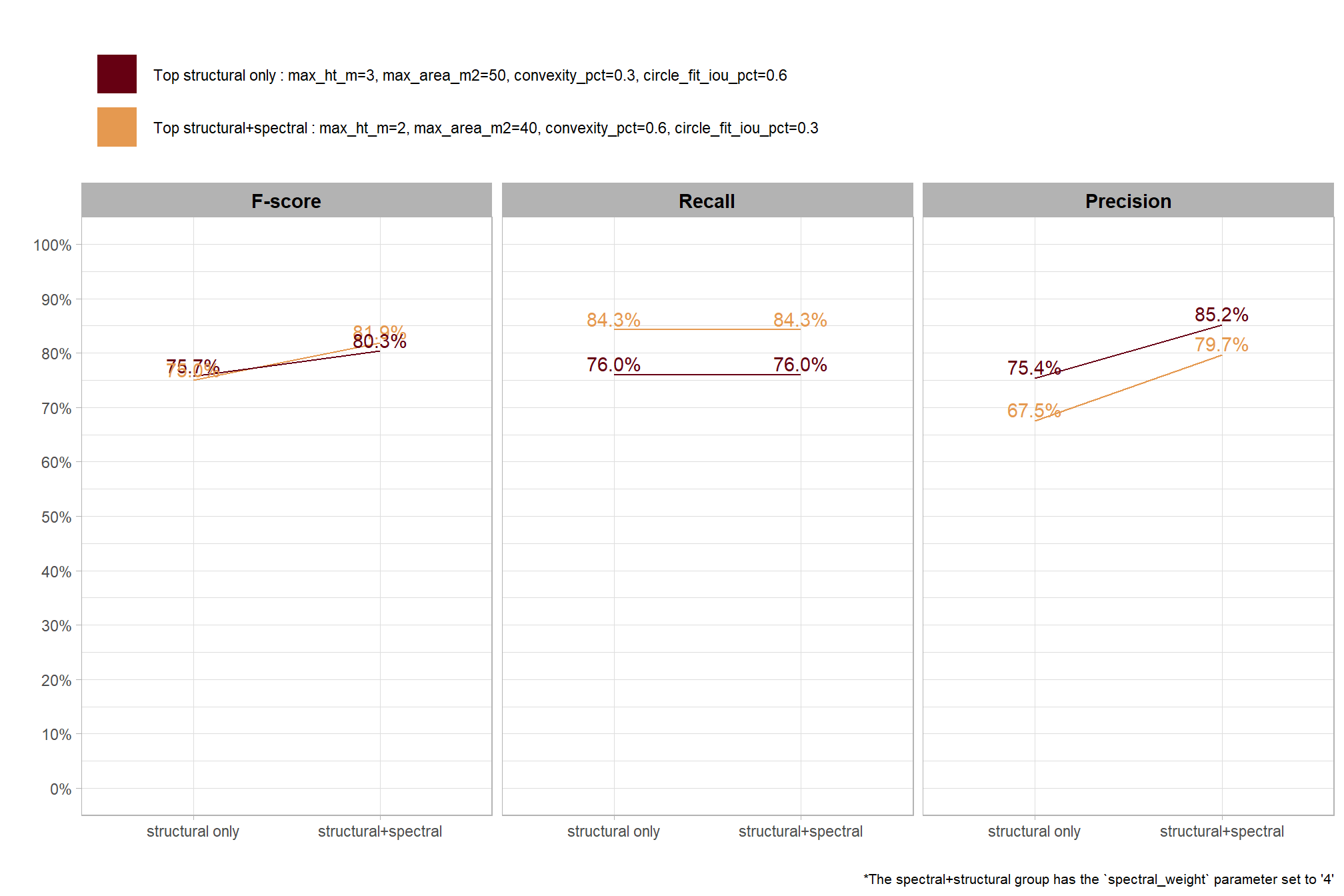
table it
# table it
combos_df_temp %>%
  dplyr::ungroup() %>%
  dplyr::select(c(
    desc,spectral_weight_fact
    ,f_score, recall, precision
  )) %>%
  dplyr::mutate(dplyr::across(
    .cols = c(f_score, recall, precision)
    , .fn = ~ scales::percent(.x, accuracy = 1)
  )) %>%
  dplyr::arrange(desc,spectral_weight_fact) %>%
  kableExtra::kbl(
    caption = paste0(
      "parameter combinations that achieved the best slash pile detection results"
    )
    , col.names = c(
      "."
      , "method"
      , "F-score", "Recall", "Precision"
    )
    , escape = F
  ) %>%
  kableExtra::kable_styling(font_size = 12) %>%
  kableExtra::collapse_rows(columns = 1, valign = "top") %>%
  kableExtra::add_header_above(c(" "=2, "Evaluation Metric" = 3)) %>%
  kableExtra::footnote(
    symbol = paste0(
      "the spectral+structural group has the `spectral_weight` parameter set to '"
      , best_spectral_weight, "'"
    )
)| . | method | F-score | Recall | Precision |
|---|---|---|---|---|
| Top structural only : max_ht_m=3, max_area_m2=50, convexity_pct=0.3, circle_fit_iou_pct=0.6 | structural only | 76% | 76% | 75% |
| structural+spectral | 80% | 76% | 85% | |
| Top structural+spectral : max_ht_m=2, max_area_m2=40, convexity_pct=0.6, circle_fit_iou_pct=0.3 | structural only | 75% | 84% | 68% |
| structural+spectral | 82% | 84% | 80% | |
* the spectral+structural group has the spectral_weight parameter set to ‘4’
|
# param_combos_spectral_gt_agg %>%
#   dplyr::filter(spectral_weight==2) %>%
#   dplyr::arrange(desc(f_score),desc(recall),pct_diff_volume_field_mape,pct_diff_area_field_mape,pct_diff_height_mape) %>%
#   dplyr::slice(1) %>%
#   dplyr::select(
#     max_ht_m
#       , max_area_m2
#       , convexity_pct
#       , circle_fit_iou_pct
#   )
looking at the best-performing methods:
- the top structural-only method achieved an F-score of 76%
- when spectral data was included with
spectral_weightof “4”, the F-score for this same structural setting increased to 80% - the absolute best-performing method using both structural and spectral data with
spectral_weightof “4” achieved an F-score of 82%
this clearly demonstrates the value of integrating spectral information for more accurate slash pile detection
8.3.6 Best results: quantification accuracy
we can cut to the chase and just look at the parameter combinations that achieved the best results based on the form quantification accuracy metrics
pct_rank_th_temp <- 0.99
df_temp <-
  param_combos_spectral_gt_agg %>%
  dplyr::arrange(pct_diff_volume_field_mape, pct_diff_diameter_mape, pct_diff_area_field_mape, pct_diff_height_mape) %>%
  dplyr::mutate(
    # label combining params
    lab = stringr::str_c(max_ht_m,max_area_m2,convexity_pct,circle_fit_iou_pct,spectral_weight, sep = ":")
    , dplyr::across(
      .cols = c(tidyselect::ends_with("_mape"))
      , .fn = dplyr::percent_rank
      , .names = "pct_rank_{.col}"
    )
  ) %>%
  # dplyr::arrange(pct_diff_paraboloid_volume_field_mape) %>%
  # dplyr::select(pct_diff_diameter_mape, pct_rank_pct_diff_paraboloid_volume_field_mape) %>%
  # now get the max of these pct ranks by row
  dplyr::rowwise() %>%
  dplyr::mutate(
    pct_rank_min = min(
      dplyr::c_across(
        tidyselect::starts_with("pct_rank")
      )
      , na.rm = T
    )
  ) %>%
  dplyr::ungroup() %>%
  dplyr::filter(pct_rank_min<=(1-pct_rank_th_temp)) %>%
  dplyr::select(
    max_ht_m,max_area_m2,convexity_pct,circle_fit_iou_pct,spectral_weight
    , lab
    , tidyselect::starts_with("pct_rank")
    , tidyselect::starts_with("pct_diff")
    , -c(pct_rank_min)
  ) %>%
  # get sort for lab
  dplyr::group_by(lab) %>%
  dplyr::mutate(sort_lab = pct_rank_pct_diff_volume_field_mape) %>%
  dplyr::ungroup() %>%
  # expand data to unique lab, pct_rank
  tidyr::pivot_longer(
    cols = tidyselect::starts_with("pct_rank")
    , names_to = "metric"
    , values_to = "value"
  ) %>%
  # keep only relevant records
  dplyr::filter(value<=(1-pct_rank_th_temp)) %>%
  dplyr::group_by(metric) %>%
  dplyr::arrange(pct_diff_volume_field_mape, pct_diff_diameter_mape, pct_diff_area_field_mape, pct_diff_height_mape) %>%
  dplyr::filter(dplyr::row_number()<=12) %>%
  dplyr::ungroup() %>%
  dplyr::mutate(
    rank_lab = stringr::str_remove(metric,"pct_rank_") %>%
      factor(
        ordered = T
        , levels = c(
          "pct_diff_volume_field_mape"
          , "pct_diff_paraboloid_volume_field_mape"
          , "pct_diff_area_field_mape"
          , "pct_diff_height_mape"
          , "pct_diff_diameter_mape"
        )
        , labels = c(
          paste0("top ", scales::percent(1-pct_rank_th_temp, accuracy = 1), " MAPE Volume irregular") %>% stringr::str_wrap(width = 14)
          , paste0("top ", scales::percent(1-pct_rank_th_temp, accuracy = 1), " MAPE Volume paraboloid") %>% stringr::str_wrap(width = 14)
          , paste0("top ", scales::percent(1-pct_rank_th_temp, accuracy = 1), " MAPE Area") %>% stringr::str_wrap(width = 14)
          , paste0("top ", scales::percent(1-pct_rank_th_temp, accuracy = 1), " MAPE Height") %>% stringr::str_wrap(width = 14)
          , paste0("top ", scales::percent(1-pct_rank_th_temp, accuracy = 1), " MAPE Diameter") %>% stringr::str_wrap(width = 14)
        )
      )
  ) %>%
  dplyr::group_by(rank_lab) %>%
  dplyr::arrange(value) %>%
  dplyr::filter(dplyr::row_number()<=12) %>%
  dplyr::select(-c(metric,value)) %>%
  dplyr::ungroup()

  # View()
# df_temp %>% dplyr::glimpse()

df_temp %>%
  tidyr::pivot_longer(
    cols = tidyselect::starts_with("pct_diff_")
    , names_to = "metric"
    , values_to = "value"
  ) %>%
  dplyr::mutate(
    metric = dplyr::case_when(
        metric == "pct_diff_volume_field_mape" ~ 1
        , metric == "pct_diff_paraboloid_volume_field_mape" ~ 2
        , metric == "pct_diff_area_field_mape" ~ 3
        , metric == "pct_diff_height_mape" ~ 4
        , metric == "pct_diff_diameter_mape" ~ 5
      ) %>%
      factor(
        ordered = T
        , levels = 1:5
        , labels = c(
          "MAPE Volume irregular"
          , "MAPE Volume paraboloid"
          , "MAPE Area"
          , "MAPE Height"
          , "MAPE Diameter"
        )
      )
    , lab = forcats::fct_reorder(lab, sort_lab) %>% forcats::fct_rev()
    , val_lab = scales::percent(value, accuracy = 0.1)
  ) %>%
  ggplot2::ggplot(
    mapping = ggplot2::aes(x = value, y = lab, fill = metric, label = val_lab)
  ) +
  ggplot2::geom_col(width = 0.6) +
  ggplot2::geom_text(color = "black", size = 2, hjust = -0.2) +
  ggplot2::scale_fill_viridis_d(option = "turbo") +
  # ggplot2::scale_fill_manual(values = pal_get_pairs_fn(6)[1:5][c(1,3,5)]) +
  ggplot2::scale_x_continuous(
    labels = scales::percent_format(accuracy = 1)
    , limits = c(0,1.05)
    # , expand = expansion(mult = c(0, .08))
  ) +
  ggplot2::facet_grid(cols = dplyr::vars(metric), rows = dplyr::vars(rank_lab), scales = "free_y") +
  ggplot2::labs(
    x = "", y = "max_ht_m : max_area_m2 : convexity_pct : circle_fit_iou_pct : spectral_weight"
    , fill = ""
    , subtitle = paste0(
       "pile shape quantification accuracy for top "
       , scales::percent(1-pct_rank_th_temp,accuracy=1)
       , " of parameter combinations"
    )
  ) +
  ggplot2::theme_light() +
  ggplot2::theme(
    legend.position = "none"
    , strip.text = ggplot2::element_text(size = 11, color = "black", face = "bold")
    , axis.text = ggplot2::element_text(size = 6)
  )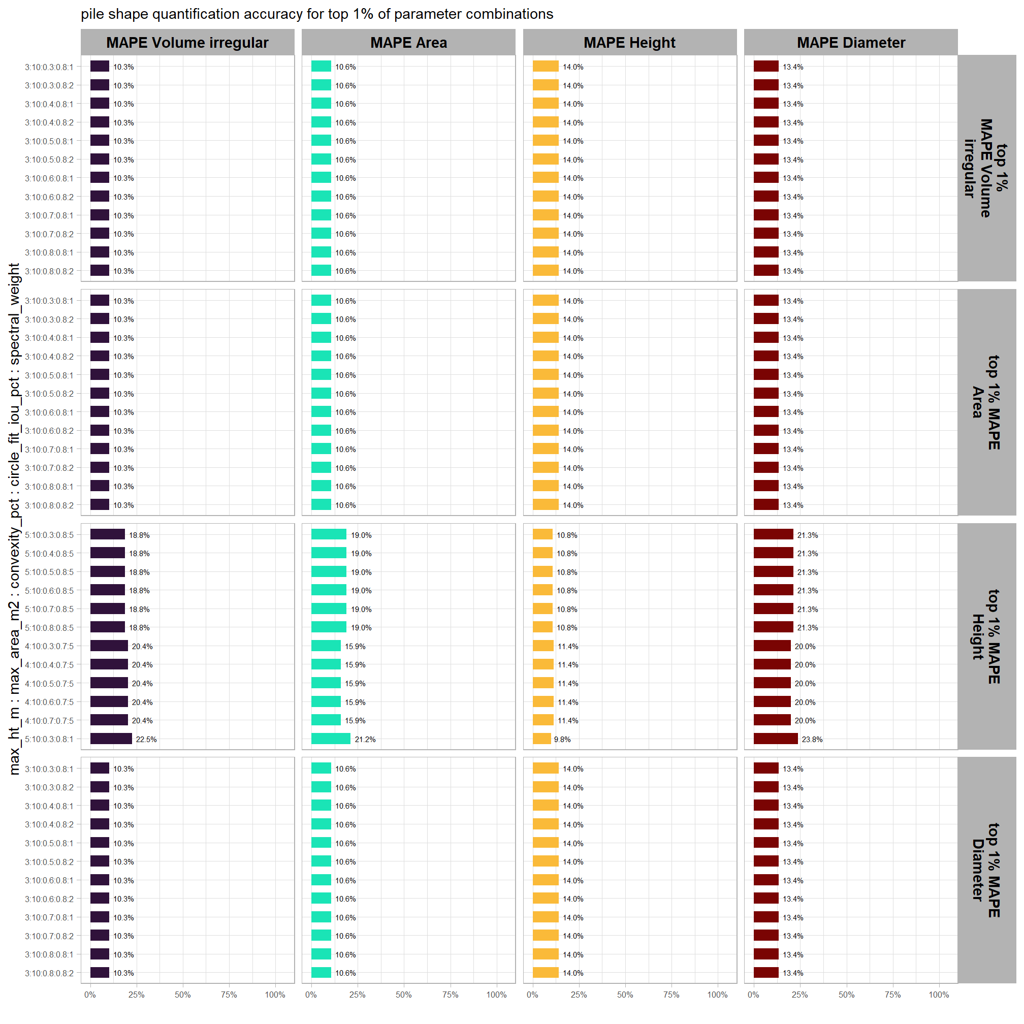
glancing at the values of the spectral_weight parameter for this set indicates that there may not be overlap between the best parameter combinations for detecting slash piles and the combinations the best estimate pile form. this is the same result we saw when using only the structural data for detecting and quantifying slash piles (see here). we’ll explore this further in the next section.
let’s make a table of these results
df_temp %>%
  dplyr::select(
    rank_lab
    , max_ht_m,max_area_m2,convexity_pct,circle_fit_iou_pct,spectral_weight
    , pct_diff_volume_field_mape, pct_diff_area_field_mape, pct_diff_height_mape, pct_diff_diameter_mape
  ) %>%
  dplyr::ungroup() %>%
  dplyr::arrange(rank_lab,pct_diff_volume_field_mape, pct_diff_area_field_mape, pct_diff_height_mape, pct_diff_diameter_mape) %>%
  dplyr::mutate(dplyr::across(
    .cols = tidyselect::starts_with("pct_diff_")
    , .fn = ~ scales::percent(.x, accuracy = 1)
  )) %>%
  dplyr::mutate(blank= "   " ) %>%
  dplyr::relocate(blank, .before = pct_diff_volume_field_mape) %>%
  kableExtra::kbl(
    caption = "parameter combinations that achieved the best slash pile form quantification results"
    , col.names = c(
      "."
      ,"max_ht_m","max_area_m2","convexity_pct","circle_fit_iou_pct","spectral_weight"
      , "   "
      , "MAPE Volume irregular"
      , "MAPE Area"
      , "MAPE Height"
      , "MAPE Diameter"
    )
    , escape = F
  ) %>%
  kableExtra::kable_styling(font_size = 11) %>%
  kableExtra::collapse_rows(columns = 1, valign = "top") %>%
kableExtra::add_header_above(c(" "=7, "Evaluation Metric" = 4))| . | max_ht_m | max_area_m2 | convexity_pct | circle_fit_iou_pct | spectral_weight | MAPE Volume irregular | MAPE Area | MAPE Height | MAPE Diameter | |
|---|---|---|---|---|---|---|---|---|---|---|
| top 1% MAPE Volume irregular | 3 | 10 | 0.3 | 0.8 | 1 | 10% | 11% | 14% | 13% | |
| 3 | 10 | 0.4 | 0.8 | 1 | 10% | 11% | 14% | 13% | ||
| 3 | 10 | 0.5 | 0.8 | 1 | 10% | 11% | 14% | 13% | ||
| 3 | 10 | 0.6 | 0.8 | 1 | 10% | 11% | 14% | 13% | ||
| 3 | 10 | 0.7 | 0.8 | 1 | 10% | 11% | 14% | 13% | ||
| 3 | 10 | 0.8 | 0.8 | 1 | 10% | 11% | 14% | 13% | ||
| 3 | 10 | 0.3 | 0.8 | 2 | 10% | 11% | 14% | 13% | ||
| 3 | 10 | 0.4 | 0.8 | 2 | 10% | 11% | 14% | 13% | ||
| 3 | 10 | 0.5 | 0.8 | 2 | 10% | 11% | 14% | 13% | ||
| 3 | 10 | 0.6 | 0.8 | 2 | 10% | 11% | 14% | 13% | ||
| 3 | 10 | 0.7 | 0.8 | 2 | 10% | 11% | 14% | 13% | ||
| 3 | 10 | 0.8 | 0.8 | 2 | 10% | 11% | 14% | 13% | ||
| top 1% MAPE Area | 3 | 10 | 0.3 | 0.8 | 1 | 10% | 11% | 14% | 13% | |
| 3 | 10 | 0.4 | 0.8 | 1 | 10% | 11% | 14% | 13% | ||
| 3 | 10 | 0.5 | 0.8 | 1 | 10% | 11% | 14% | 13% | ||
| 3 | 10 | 0.6 | 0.8 | 1 | 10% | 11% | 14% | 13% | ||
| 3 | 10 | 0.7 | 0.8 | 1 | 10% | 11% | 14% | 13% | ||
| 3 | 10 | 0.8 | 0.8 | 1 | 10% | 11% | 14% | 13% | ||
| 3 | 10 | 0.3 | 0.8 | 2 | 10% | 11% | 14% | 13% | ||
| 3 | 10 | 0.4 | 0.8 | 2 | 10% | 11% | 14% | 13% | ||
| 3 | 10 | 0.5 | 0.8 | 2 | 10% | 11% | 14% | 13% | ||
| 3 | 10 | 0.6 | 0.8 | 2 | 10% | 11% | 14% | 13% | ||
| 3 | 10 | 0.7 | 0.8 | 2 | 10% | 11% | 14% | 13% | ||
| 3 | 10 | 0.8 | 0.8 | 2 | 10% | 11% | 14% | 13% | ||
| top 1% MAPE Height | 5 | 10 | 0.3 | 0.8 | 5 | 19% | 19% | 11% | 21% | |
| 5 | 10 | 0.4 | 0.8 | 5 | 19% | 19% | 11% | 21% | ||
| 5 | 10 | 0.5 | 0.8 | 5 | 19% | 19% | 11% | 21% | ||
| 5 | 10 | 0.6 | 0.8 | 5 | 19% | 19% | 11% | 21% | ||
| 5 | 10 | 0.7 | 0.8 | 5 | 19% | 19% | 11% | 21% | ||
| 5 | 10 | 0.8 | 0.8 | 5 | 19% | 19% | 11% | 21% | ||
| 4 | 10 | 0.3 | 0.7 | 5 | 20% | 16% | 11% | 20% | ||
| 4 | 10 | 0.4 | 0.7 | 5 | 20% | 16% | 11% | 20% | ||
| 4 | 10 | 0.5 | 0.7 | 5 | 20% | 16% | 11% | 20% | ||
| 4 | 10 | 0.6 | 0.7 | 5 | 20% | 16% | 11% | 20% | ||
| 4 | 10 | 0.7 | 0.7 | 5 | 20% | 16% | 11% | 20% | ||
| 5 | 10 | 0.3 | 0.8 | 1 | 23% | 21% | 10% | 24% | ||
| top 1% MAPE Diameter | 3 | 10 | 0.3 | 0.8 | 1 | 10% | 11% | 14% | 13% | |
| 3 | 10 | 0.4 | 0.8 | 1 | 10% | 11% | 14% | 13% | ||
| 3 | 10 | 0.5 | 0.8 | 1 | 10% | 11% | 14% | 13% | ||
| 3 | 10 | 0.6 | 0.8 | 1 | 10% | 11% | 14% | 13% | ||
| 3 | 10 | 0.7 | 0.8 | 1 | 10% | 11% | 14% | 13% | ||
| 3 | 10 | 0.8 | 0.8 | 1 | 10% | 11% | 14% | 13% | ||
| 3 | 10 | 0.3 | 0.8 | 2 | 10% | 11% | 14% | 13% | ||
| 3 | 10 | 0.4 | 0.8 | 2 | 10% | 11% | 14% | 13% | ||
| 3 | 10 | 0.5 | 0.8 | 2 | 10% | 11% | 14% | 13% | ||
| 3 | 10 | 0.6 | 0.8 | 2 | 10% | 11% | 14% | 13% | ||
| 3 | 10 | 0.7 | 0.8 | 2 | 10% | 11% | 14% | 13% | ||
| 3 | 10 | 0.8 | 0.8 | 2 | 10% | 11% | 14% | 13% |
let’s use the value of spectral_weight that most frequently results in the best pile detection based on F-score (“4”) to compare results to not using any spectral data (i.e. just using structural data as outlined in our method here). We’ll then average across all other factors to look at the main effect of spectral_weight after creating a dichotomous factor of structural only versus structural+spectral
# quick mod
dep_vars_temp <- c("pct_diff_volume_field_mape", "pct_diff_area_field_mape", "pct_diff_height_mape", "pct_diff_diameter_mape")
# list of formulas
formulas_temp <- dep_vars_temp %>%
  purrr::map(~stats::reformulate(c("spectral_weight_fact","-1"), response = .x))
names(formulas_temp) <- dep_vars_temp
# formulas_temp
models_temp <- formulas_temp %>%
  purrr::map(\(x) lm(formula = x, data = combos_df_temp))
names(models_temp) <- dep_vars_temp
# models_temp
# combine into df
pred_df_temp <- purrr::map_df(models_temp, broom::tidy, .id = "metric") %>%
  dplyr::select(-c(statistic)) %>%
  dplyr::mutate(
    dep_var = dplyr::case_when(
        metric == "pct_diff_volume_field_mape" ~ 1
        , metric == "pct_diff_paraboloid_volume_field_mape" ~ 2
        , metric == "pct_diff_area_field_mape" ~ 3
        , metric == "pct_diff_height_mape" ~ 4
        , metric == "pct_diff_diameter_mape" ~ 5
      ) %>%
      factor(
        ordered = T
        , levels = 1:5
        , labels = c(
          "MAPE Volume irregular"
          , "MAPE Volume paraboloid"
          , "MAPE Area field"
          , "MAPE Height"
          , "MAPE Diameter"
        )
      )
    , term = stringr::str_remove_all(term, "spectral_weight_fact") %>% factor()
    # to obtain the 95% confidence interval...
      # ...1.96 times the standard error is added and subtracted from the sample mean
    , ul = estimate+std.error*1.96
    , ll = estimate-std.error*1.96
  ) %>%
  dplyr::rename(spectral_weight_fact=term) %>%
  dplyr::relocate(dep_var) %>%
  dplyr::arrange(dep_var,spectral_weight_fact)

# pred_df_temp
# table it
pred_df_temp %>%
  dplyr::select(-c(metric,ul,ll)) %>%
  dplyr::mutate(
    estimate = scales::percent(estimate, accuracy = 0.1)
    , std.error = scales::percent(std.error, accuracy = 0.01)
    , p.value = ifelse(
        p.value < 0.001
        , "< 0.001"
        , scales::comma(p.value, accuracy = 0.0001)
      )
  ) %>%
  kableExtra::kbl(
    caption = "Predictions for quantification accuracy metrics by detection method<br>averaging across all other structural detection parameters"
    , col.names = c(".","method","predicted mean", "SE", "p-value")
  ) %>%
  kableExtra::kable_styling() %>%
kableExtra::collapse_rows(columns = 1, valign = "top")| . | method | predicted mean | SE | p-value |
|---|---|---|---|---|
| MAPE Volume irregular | structural only | 31.2% | 0.36% | < 0.001 |
| structural+spectral | 31.2% | 0.36% | < 0.001 | |
| MAPE Area field | structural only | 23.9% | 0.55% | < 0.001 |
| structural+spectral | 23.9% | 0.55% | < 0.001 | |
| MAPE Height | structural only | 16.6% | 1.68% | 0.0101 |
| structural+spectral | 16.6% | 1.68% | 0.0101 | |
| MAPE Diameter | structural only | 25.6% | 0.31% | < 0.001 |
| structural+spectral | 25.6% | 0.31% | < 0.001 |
the spectral data does not alter the quantification of slash pile form. this is because spectral information is used solely to filter candidate piles, meaning it neither reshapes existing ones nor introduces new detections.
8.3.7 Best results: detection & quantification
as we saw in the sensitivity testing of the structural detection methodology (here), there was not a clear a relationship between the quantification and detection accuracy metrics
we need to find the parameter combinations that result in the best balanced detection and quantification accuracy
param_combos_spectral_gt_agg %>%
  dplyr::ungroup() %>%
  dplyr::select(
    rn,max_ht_m,max_area_m2,convexity_pct,circle_fit_iou_pct,spectral_weight
    , f_score
    # quantification accuracy
    , tidyselect::ends_with("_mape")
  ) %>%
  tidyr::pivot_longer(
    cols = c(tidyselect::ends_with("_mape"))
    , names_to = "metric"
    , values_to = "value"
  ) %>%
  dplyr::mutate(
    eval_metric = stringr::str_extract(metric, "(_rmse|_rrmse|_mean|_mape)$") %>%
      stringr::str_remove_all("_") %>%
      stringr::str_replace_all("mean","me") %>%
      toupper() %>%
      factor(
        ordered = T
        , levels = c("ME","RMSE","RRMSE","MAPE")
      )
    , pile_metric = metric %>%
      stringr::str_remove("(_rmse|_rrmse|_mean|_mape)$") %>%
      stringr::str_extract("(paraboloid_volume|volume|area|height|diameter)") %>%
      factor(
        ordered = T
        , levels = c(
          "volume"
          , "paraboloid_volume"
          , "area"
          , "height"
          , "diameter"
        )
        , labels = c(
          "Volume"
          , "Volume paraboloid"
          , "Area"
          , "Height"
          , "Diameter"
        )
      )
  ) %>%
  # plot
  ggplot2::ggplot(mapping = ggplot2::aes(x = f_score, y = value, color = pile_metric)) +
  ggplot2::geom_point() +
  ggplot2::facet_wrap(facets = dplyr::vars(pile_metric)) +
  ggplot2::scale_color_viridis_d(option = "turbo") +
  ggplot2::scale_x_continuous(
    labels = scales::percent_format(accuracy = 1)
    , limits = c(0,1)
  ) +
  ggplot2::scale_y_continuous(
    labels = scales::percent_format(accuracy = 1)
    , limits = c(0,NA)
  ) +
  ggplot2::labs(x = "F-Score", y = "MAPE") +
  ggplot2::theme_light() +
  ggplot2::theme(
    legend.position = "none"
    , strip.text = ggplot2::element_text(size = 11, color = "black", face = "bold")
  )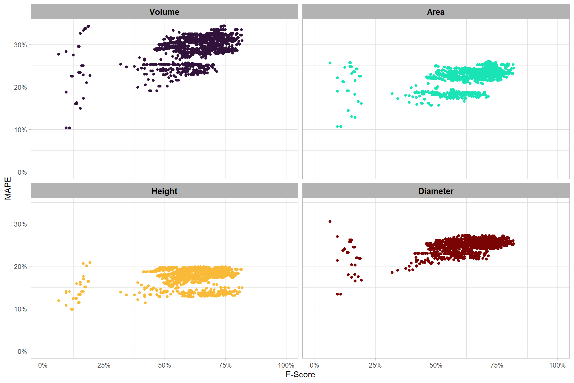
aside from a distinct cluster of points at the lower end of the F-Score range, there does not appear to be a relationship between the pile form quantification and detection accuracy metrics
let’s look at only parameter combinations that are among the best in both detection and form quantification accuracy
we’ll use the F-Score and the average rank of the MAPE metrics across all form measurements to determine the best overall list
df_temp <-
  param_combos_spectral_gt_agg %>%
  # dplyr::select(c(tidyselect::ends_with("_mape") & tidyselect::contains("volume"))) %>% names()
  dplyr::mutate(
    # label combining params
    lab = stringr::str_c(max_ht_m,max_area_m2,convexity_pct,circle_fit_iou_pct,spectral_weight, sep = ":")
    , dplyr::across(
      .cols = c(tidyselect::ends_with("_mape"))
      # .cols = c(tidyselect::ends_with("_mape") & tidyselect::contains("volume"))
      , .fn = ~dplyr::percent_rank(-.x)
      , .names = "pct_rank_quant_{.col}"
    )
    , dplyr::across(
      .cols = c(f_score)
      # .cols = c(f_score,recall)
      , .fn = ~dplyr::percent_rank(.x)
      , .names = "pct_rank_det_{.col}"
    )
  ) %>%
  # dplyr::arrange(pct_diff_paraboloid_volume_field_mape) %>%
  # dplyr::select(pct_diff_diameter_mape, pct_rank_pct_diff_paraboloid_volume_field_mape) %>%
  # View()
  # now get the max of these pct ranks by row
  dplyr::rowwise() %>%
  dplyr::mutate(
    pct_rank_quant_mean = mean(
      dplyr::c_across(
        tidyselect::starts_with("pct_rank_quant_")
      )
      , na.rm = T
    )
    , pct_rank_det_mean = mean(
      dplyr::c_across(
        tidyselect::starts_with("pct_rank_det_")
      )
      , na.rm = T
    )
  ) %>%
  dplyr::ungroup() %>%
  # now make quadrant var
  dplyr::mutate(
    # this is for the quadrant plot
    overall_accuracy = dplyr::case_when(
      pct_rank_det_mean>=0.95 & pct_rank_quant_mean>=0.95 ~ 1
      , pct_rank_det_mean>=0.90 & pct_rank_quant_mean>=0.90 ~ 2
      , pct_rank_det_mean>=0.75 & pct_rank_quant_mean>=0.75 ~ 3
      , pct_rank_det_mean>=0.50 & pct_rank_quant_mean>=0.50 ~ 4
      , pct_rank_det_mean>=0.50 & pct_rank_quant_mean<0.50 ~ 5
      , pct_rank_det_mean<0.50 & pct_rank_quant_mean>=0.50 ~ 6
      , T ~ 7
    ) %>%
    factor(
      ordered = T
      , levels = 1:7
      , labels = c(
        "top 5% detection & quantification" # pct_rank_mean>=0.95 & pct_rank_f_score>=0.95 ~ 1
        , "top 10% detection & quantification" # pct_rank_mean>=0.90 & pct_rank_f_score>=0.90 ~ 2
        , "top 25% detection & quantification" # pct_rank_mean>=0.75 & pct_rank_f_score>=0.75 ~ 3
        , "top 50% detection & quantification" # pct_rank_mean>=0.50 & pct_rank_f_score>=0.50 ~ 4
        , "top 50% quantification" # pct_rank_mean>=0.50 & pct_rank_f_score<0.50 ~ 5
        , "top 50% detection" # pct_rank_mean<0.50 & pct_rank_f_score>=0.50 ~ 6
        , "bottom 50% detection & quantification"
      )
    )
  ) %>%
  dplyr::select(
    rn,max_ht_m,max_area_m2,convexity_pct,circle_fit_iou_pct,spectral_weight
    , lab
    , f_score, recall, precision
    , tidyselect::ends_with("_mape")
    , tidyselect::starts_with("pct_rank")
    , overall_accuracy
  )

# plot
df_temp %>%
  ggplot2::ggplot(
    mapping=ggplot2::aes(x = pct_rank_det_mean, y = pct_rank_quant_mean, color = overall_accuracy)
  ) +
  ggplot2::geom_vline(xintercept = 0.5, color = "gray22") +
  ggplot2::geom_hline(yintercept = 0.5, color = "gray22") +
  ggplot2::geom_vline(xintercept = 0.75, color = "gray44") +
  ggplot2::geom_hline(yintercept = 0.75, color = "gray44") +
  ggplot2::geom_vline(xintercept = 0.9, color = "gray66") +
  ggplot2::geom_hline(yintercept = 0.9, color = "gray66") +
  ggplot2::geom_point() +
  ggplot2::scale_colour_viridis_d(option = "inferno", end = 0.8, direction = -1) +
  ggplot2::scale_x_continuous(
    labels = scales::percent_format(accuracy = 1)
    , limits = c(0,1)
  ) +
  ggplot2::scale_y_continuous(
    labels = scales::percent_format(accuracy = 1)
    , limits = c(0,1)
  ) +
  ggplot2::labs(
    x = "Percentile F-Score", y = "Percentile MAPE (mean)"
    , color = ""
  ) +
  ggplot2::theme_light() +
  ggplot2::theme(
    legend.position = "bottom"
    , legend.text = ggplot2::element_text(size = 8)
    , strip.text = ggplot2::element_text(size = 11, color = "black", face = "bold")
    , axis.text = ggplot2::element_text(size = 7)
  ) +
  ggplot2::guides(
    color = ggplot2::guide_legend(override.aes = list(shape = 15, linetype = 0, size = 5, alpha = 1))
    , shape = "none"
  )
before we look at the parameter combinations that are in the upper-right of the quadrant plot, let’s color this by the spectral_weight parameter to look for patterns
# plot
df_temp %>%
  ggplot2::ggplot(
    mapping=ggplot2::aes(x = pct_rank_det_mean, y = pct_rank_quant_mean, color = factor(spectral_weight))
  ) +
  ggplot2::geom_vline(xintercept = 0.5, color = "gray22") +
  ggplot2::geom_hline(yintercept = 0.5, color = "gray22") +
  ggplot2::geom_vline(xintercept = 0.75, color = "gray44") +
  ggplot2::geom_hline(yintercept = 0.75, color = "gray44") +
  ggplot2::geom_vline(xintercept = 0.9, color = "gray66") +
  ggplot2::geom_hline(yintercept = 0.9, color = "gray66") +
  ggplot2::geom_point() +
  ggplot2::scale_color_viridis_d(begin = 0.1,end=0.9) +
  # ggplot2::scale_colour_viridis_d(option = "viridis", end = 0.8, direction = -1) +
  ggplot2::scale_x_continuous(
    labels = scales::percent_format(accuracy = 1)
    , limits = c(0,1)
  ) +
  ggplot2::scale_y_continuous(
    labels = scales::percent_format(accuracy = 1)
    , limits = c(0,1)
  ) +
  ggplot2::labs(
    x = "Percentile F-Score", y = "Percentile MAPE (mean)"
    , color = "spectral_weight"
  ) +
  ggplot2::theme_light() +
  ggplot2::theme(
    legend.position = "bottom"
    , legend.text = ggplot2::element_text(size = 8)
    , strip.text = ggplot2::element_text(size = 11, color = "black", face = "bold")
    , axis.text = ggplot2::element_text(size = 7)
  ) +
  ggplot2::guides(
    color = ggplot2::guide_legend(override.aes = list(shape = 15, linetype = 0, size = 5, alpha = 1))
    , shape = "none"
  )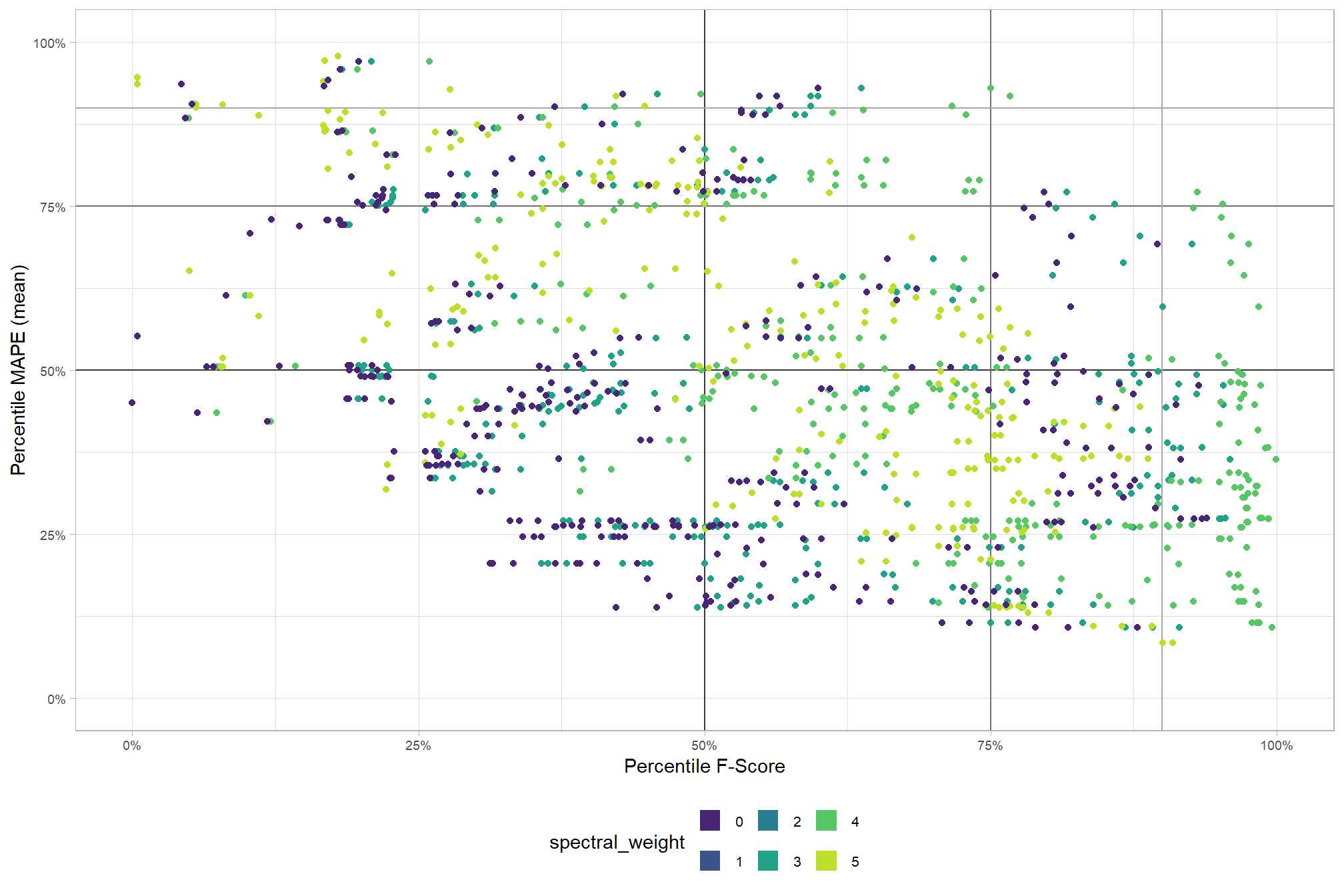
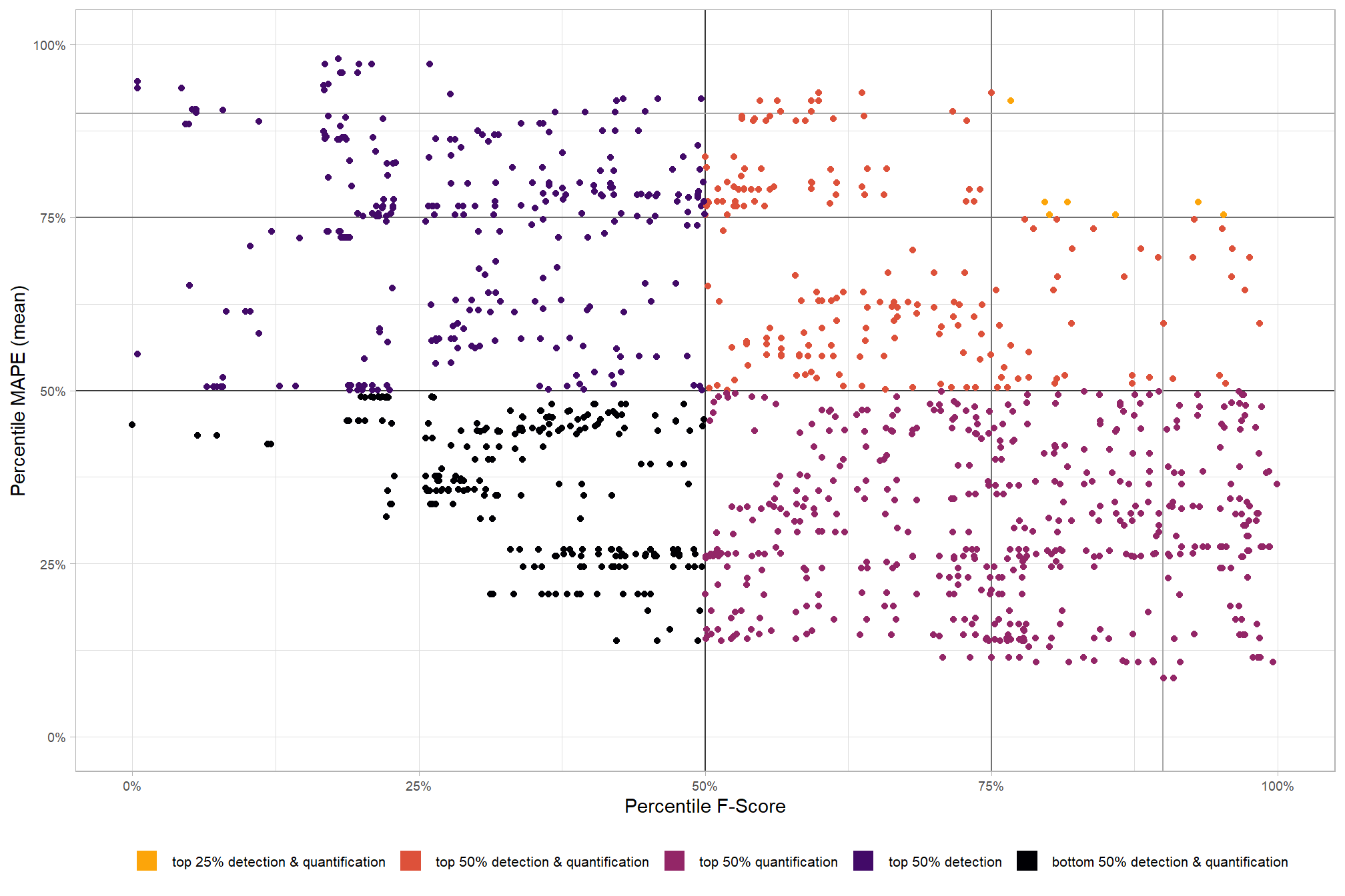
as we already discovered from our investigation of the top performing method based on pile detection accuracy, having the spectral_weight parameter set to 3, 4, or 5 results in the best detection. the upper right of this quadrant plot reveals that some of these top performing methods for detecting piles also result in relatively accurate pile form quantification
let’s look at the parameter combinations that are in the upper-right of the quadrant plot. That is, the parameter combinations that performed best at both pile detection accuracy and pile form quantification accuracy
# filter
df_temp <- df_temp %>%
  dplyr::filter(
    pct_rank_det_mean>=0.75 & pct_rank_quant_mean>=0.75
  ) %>%
  # nrow()
  dplyr::mutate(
    pct_rank_overall = (pct_rank_det_mean+pct_rank_quant_mean)/2
    , lab = forcats::fct_reorder(lab, pct_rank_overall)
  ) %>%
  dplyr::arrange(desc(pct_rank_overall)) %>%
  dplyr::mutate(rank_overall = dplyr::row_number())
# save the best overall param_combo_df record numbers
best_pile_detect_spectral_rn <- df_temp %>%
  dplyr::distinct(rn,spectral_weight,lab,rank_overall,pct_rank_overall,pct_rank_det_mean,pct_rank_quant_mean)
# best_pile_detect_spectral_rn %>% dplyr::glimpse()
param_combos_spectral_gt_agg %>%
dplyr::ungroup() %>%
# filter for the best
dplyr::left_join(
best_pile_detect_spectral_rn %>% dplyr::distinct(rn,spectral_weight) %>% dplyr::mutate(is_best=T)
, by = dplyr::join_by(rn,spectral_weight)
, relationship = "one-to-one"
) %>%
dplyr::mutate(is_best = dplyr::coalesce(is_best,F)) %>%
dplyr::select(
rn,max_ht_m,max_area_m2,convexity_pct,circle_fit_iou_pct,spectral_weight
, is_best
, f_score
# quantification accuracy
, tidyselect::ends_with("_mape")
) %>%
tidyr::pivot_longer(
cols = c(tidyselect::ends_with("_mape"))
, names_to = "metric"
, values_to = "value"
) %>%
dplyr::mutate(
eval_metric = stringr::str_extract(metric, "(_rmse|_rrmse|_mean|_mape)$") %>%
stringr::str_remove_all("_") %>%
stringr::str_replace_all("mean","me") %>%
toupper() %>%
factor(
ordered = T
, levels = c("ME","RMSE","RRMSE","MAPE")
)
, pile_metric = metric %>%
stringr::str_remove("(_rmse|_rrmse|_mean|_mape)$") %>%
stringr::str_extract("(paraboloid_volume|volume|area|height|diameter)") %>%
factor(
ordered = T
, levels = c(
"volume"
, "paraboloid_volume"
, "area"
, "height"
, "diameter"
)
, labels = c(
"Volume"
, "Volume paraboloid"
, "Area"
, "Height"
, "Diameter"
)
)
, color_metric = ifelse(is_best, pile_metric, NA) %>% factor()
) %>%
dplyr::arrange(is_best) %>%
# plot
ggplot2::ggplot(mapping = ggplot2::aes(x = f_score, y = value, color = color_metric)) +
ggplot2::geom_point() +
ggplot2::facet_wrap(facets = dplyr::vars(pile_metric)) +
ggplot2::scale_color_viridis_d(option = "turbo", na.value = "gray88") +
ggplot2::scale_x_continuous(
labels = scales::percent_format(accuracy = 1)
, limits = c(0,1)
) +
ggplot2::scale_y_continuous(
labels = scales::percent_format(accuracy = 1)
, limits = c(0,NA)
) +
ggplot2::labs(x = "F-Score", y = "MAPE", caption = "*records in gray not selected") +
ggplot2::theme_light() +
ggplot2::theme(
legend.position = "none"
, strip.text = ggplot2::element_text(size = 11, color = "black", face = "bold")
)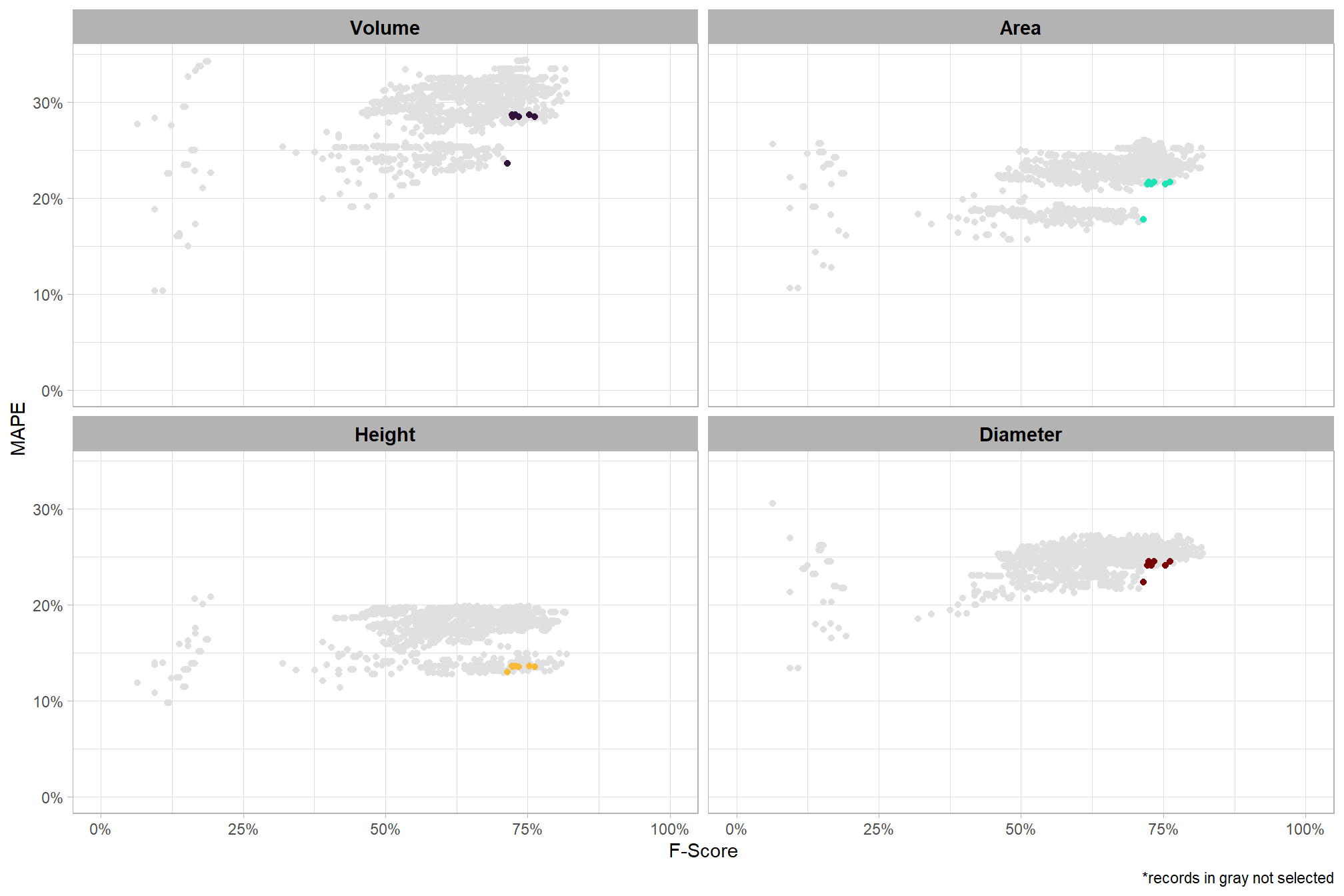
if we look at these top parameter combinations only, what can we expect regarding detection accuracy
# plot it
plt_detection_dist(
  df = param_combos_spectral_gt_agg %>%
    # filter for best of best
    dplyr::inner_join(
      best_pile_detect_spectral_rn %>% dplyr::distinct(rn,spectral_weight) %>% dplyr::mutate(is_best=T)
      , by = dplyr::join_by(rn,spectral_weight)
      , relationship = "one-to-one"
    )
  , paste0(
   "distribution of pile detection accuracy metrics for the top"
   , " (n="
   , scales::comma(nrow(best_pile_detect_spectral_rn), accuracy = 1)
   , ") "
   , "parameter combinations\nbased on both detection and quantification accuracy using structural and spectral data"
  )
)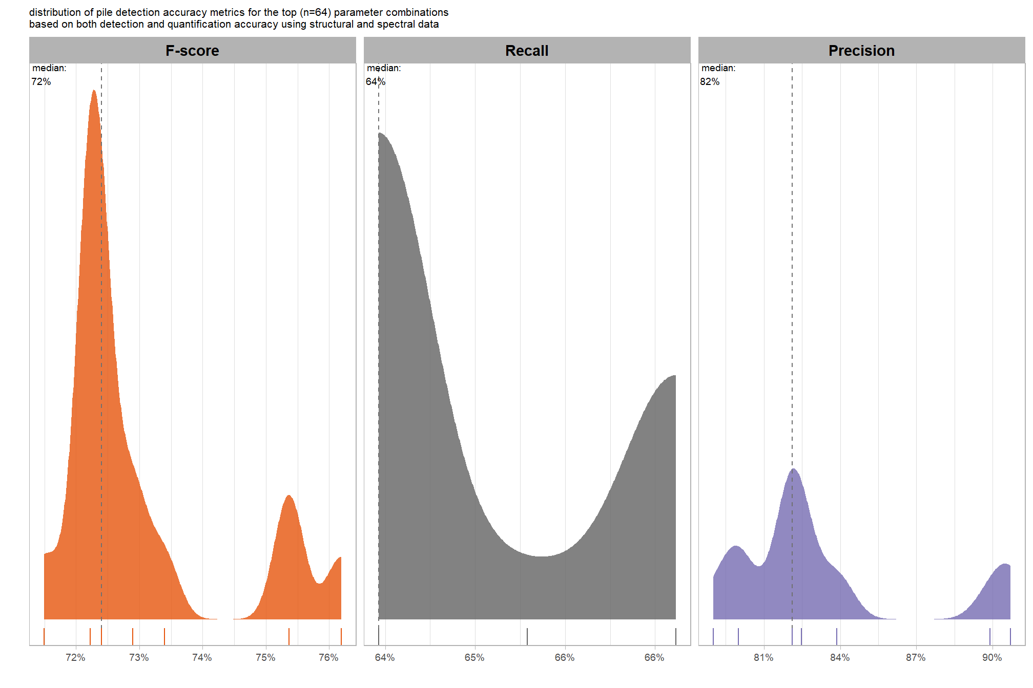
this is interesting, among the top performers in both detection (F-score) and quantification (overall MAPE), a few combinations had noticeably higher recall rates. assuming quantification accuracy is similar across this elite group, we should prioritize those with the highest recall.
but first, if we look at all these top combinations, what can we expect regarding their quantification accuracy?
# plot it
plt_form_quantification_dist(
  df = param_combos_spectral_gt_agg %>%
    dplyr::ungroup() %>%
    # filter for best of best
    dplyr::inner_join(
      best_pile_detect_spectral_rn %>% dplyr::distinct(rn,spectral_weight) %>% dplyr::mutate(is_best=T)
      , by = dplyr::join_by(rn,spectral_weight)
      , relationship = "one-to-one"
    )
  , paste0(
     "distribution of pile form quantification accuracy metrics for the top"
     # , scales::percent(1-pct_rank_th_top,accuracy=1)
     , " (n="
     , scales::comma(nrow(best_pile_detect_spectral_rn), accuracy = 1)
     , ") "
     , "parameter combinations\nbased on both detection and quantification accuracy using structural and spectral data"
  )
)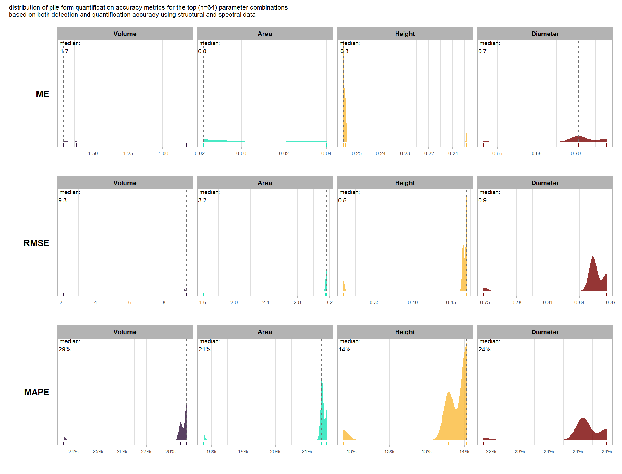
the distributions of these form quantification accuracy metrics span a narrow range, especially with respect to MAPE. as such, we’ll focus on the best overall parameter combinations that also achieved the highest recall rates
before we move on, let’s check the distribution of the spectral_weight parameter for these top performing settings
param_combos_spectral_gt_agg %>%
  dplyr::distinct(spectral_weight) %>%
  dplyr::left_join(
    best_pile_detect_spectral_rn %>%
      dplyr::count(spectral_weight)
  ) %>%
  dplyr::arrange(spectral_weight) %>%
  dplyr::mutate(
    n = dplyr::coalesce(n,0)
    , pct = scales::percent( n/sum(n), accuracy = 0.1)
  ) %>%
  kableExtra::kbl(
    caption = "spectral_weight setting of top performers in both detection (F-score) and quantification (overall MAPE)"
  ) %>%
kableExtra::kable_styling()| spectral_weight | n | pct |
|---|---|---|
| 0 | 12 | 18.8% |
| 1 | 12 | 18.8% |
| 2 | 12 | 18.8% |
| 3 | 12 | 18.8% |
| 4 | 16 | 25.0% |
| 5 | 0 | 0.0% |
where these settings in our final recommended settings when looking at the structural data only?
8.4 Final recommended settings
our final step in this sensitivity testing is to identify the best-performing parameter combinations that not only balance detection and quantification accuracy but also achieve the highest recall rates. we’ll select these by choosing any combination whose recall rate is at least two standard deviations above the average for this top group. if no combinations meet this criterion, we will instead select the top 10 combinations based on their recall rates.
# put a flag in our best_pile_detect_spectral_rn data
best_pile_detect_spectral_rn <-
  best_pile_detect_spectral_rn %>%
  dplyr::left_join(
    param_combos_spectral_gt_agg %>%
      dplyr::ungroup() %>%
      # filter for best of best
      dplyr::inner_join(
        best_pile_detect_spectral_rn %>% dplyr::distinct(rn,spectral_weight) %>% dplyr::mutate(is_best=T)
        , by = dplyr::join_by(rn,spectral_weight)
        , relationship = "one-to-one"
      ) %>%
      # check recall rate
      dplyr::arrange(desc(recall)) %>%
      dplyr::mutate(
        is_recall_above_mean = recall >= ( mean(recall) + sd(recall)*2 )
        # if no records have a recall at least one stdandard dev above the mean, just take the top ten
        , is_top_recall = dplyr::case_when(
          sum(is_recall_above_mean)>4 ~ is_recall_above_mean
          , T ~ dplyr::row_number()<=10
        )
      ) %>%
      dplyr::select(rn,spectral_weight,is_top_recall)
    , by = dplyr::join_by(rn,spectral_weight)
    , relationship = "one-to-one"
  )
# huh?
# best_pile_detect_spectral_rn %>% dplyr::glimpse()
best_pile_detect_spectral_rn %>% dplyr::count(is_top_recall)
## # A tibble: 2 × 2
## is_top_recall n
## <lgl> <int>
## 1 FALSE 54
## 2 TRUE 10finally, let’s look at the pile detection accuracy metrics at the individual parameter combination level
# pal_temp %>% scales::show_col()
# filter and reshape
df_temp <-
  param_combos_spectral_gt_agg %>%
  dplyr::ungroup() %>%
  # filter for best of best
  dplyr::inner_join(
    best_pile_detect_spectral_rn %>%
      dplyr::filter(is_top_recall) %>%
      dplyr::select(rn,spectral_weight,lab,rank_overall)
    , by = dplyr::join_by(rn,spectral_weight)
    , relationship = "one-to-one"
  ) %>%
  dplyr::select(
    max_ht_m,max_area_m2,convexity_pct,circle_fit_iou_pct,spectral_weight
    , lab
    # detection
    , f_score, recall, precision
    # quantification
    , tidyselect::ends_with("_rmse")
    , tidyselect::ends_with("_rrmse")
    , tidyselect::ends_with("_mean")
    , tidyselect::ends_with("_mape")
  ) %>%
  tidyr::pivot_longer(
    cols = c(
      f_score, recall, precision
      , tidyselect::ends_with("_rmse")
      , tidyselect::ends_with("_rrmse")
      , tidyselect::ends_with("_mean")
      , tidyselect::ends_with("_mape")
    )
    , names_to = "metric"
    , values_to = "value"
  ) %>%
  dplyr::mutate(
    eval_metric = stringr::str_extract(metric, "(_rmse|_rrmse|_mean|_mape|f_score|recall|precision)$") %>%
      stringr::str_remove_all("_") %>%
      stringr::str_replace_all("mean","me") %>%
      toupper() %>%
      factor(
        ordered = T
        , levels = c("FSCORE","RECALL","PRECISION", "ME","RMSE","RRMSE","MAPE")
        , labels = c("F-score","Recall","Precision", "ME","RMSE","RRMSE","MAPE")
      )
    , pile_metric = metric %>%
      stringr::str_remove("(_rmse|_rrmse|_mean|_mape)$") %>%
      stringr::str_extract("(paraboloid_volume|volume|area|height|diameter)") %>%
      dplyr::coalesce("detection") %>%
      factor(
        ordered = T
        , levels = c(
          "detection"
          , "volume"
          , "paraboloid_volume"
          , "area"
          , "height"
          , "diameter"
        )
        , labels = c(
          "Detection"
          , "Volume"
          , "Volume paraboloid"
          , "Area"
          , "Height"
          , "Diameter"
        )
      )
    , value_lab = dplyr::case_when(
        eval_metric %in% c("F-score","Recall","Precision", "RRMSE", "MAPE") ~ scales::percent(value,accuracy=0.1)
        , eval_metric == "ME" ~ scales::comma(value,accuracy=0.01)
        , T ~ scales::comma(value,accuracy=0.1)
      )
  ) %>%
  # make var for color
  dplyr::group_by(pile_metric, eval_metric) %>%
  dplyr::mutate(
    # for ME, color by abs...for f-score,recall,precision color by -value so that higher means better...
      # ...since higher means worse for quantification accuracy metrics
    value_dir = dplyr::case_when(
      eval_metric %in% c("ME") ~ abs(value)
      , eval_metric %in% c("F-score","Recall","Precision") ~ -value
      , T ~ value
    )
    , value_z = (value_dir-mean(value_dir,na.rm=T))/sd(value_dir,na.rm=T) # this is the key to the different colors within facets
  ) %>%
  dplyr::ungroup()

# how to plot all of this (without patchwork)?????
df_temp %>%
  dplyr::filter(!eval_metric %in% c("RRMSE")) %>%
  # View()
  ggplot2::ggplot(mapping = ggplot2::aes(x = eval_metric, y = lab)) +
  ggplot2::geom_tile(
    mapping = ggplot2::aes(fill = pile_metric, alpha = -value_z)
    , color = "gray"
  ) +
  ggplot2::geom_text(
    mapping = ggplot2::aes(label = value_lab, fontface = "bold")
    , color = "white"
  ) +
  ggplot2::facet_grid(cols = dplyr::vars(pile_metric), scales = "free_x") +
  ggplot2::scale_x_discrete(position = "top") +
  ggplot2::scale_fill_manual(values = c("gray33", viridis::turbo(n=4))) +
  ggplot2::scale_alpha_binned(range = c(0.55, 1)) + # this is the key to the different colors within facets
  ggplot2::theme_light() +
  ggplot2::labs(
    x = ""
    , y = "max_ht_m : max_area_m2 : convexity_pct : circle_fit_iou_pct : spectral_weight"
    , subtitle = paste0(
       "pile detection and form quantification accuracy metrics for the top"
       # , scales::percent(1-pct_rank_th_top,accuracy=1)
       , " (n="
       , scales::comma(sum(best_pile_detect_spectral_rn$is_top_recall,na.rm=T), accuracy = 1)
       , ") "
       , "overall parameter combinations\nbased on both detection and quantification accuracy using structural and spectral data"
      )
    , caption = "*darker colors indicate relatively higher accuracy values"
  ) +
  ggplot2::theme(
    legend.position = "none"
    , panel.grid = ggplot2::element_blank()
    , strip.placement = "outside"
    , strip.text.x = ggplot2::element_text(size = 8, color = "black", face = "bold")
    , axis.text.x = ggplot2::element_text(size = 7, color = "black", face = "bold")
    , axis.title.x = ggplot2::element_blank()
    , plot.subtitle = ggplot2::element_text(size = 8)
  )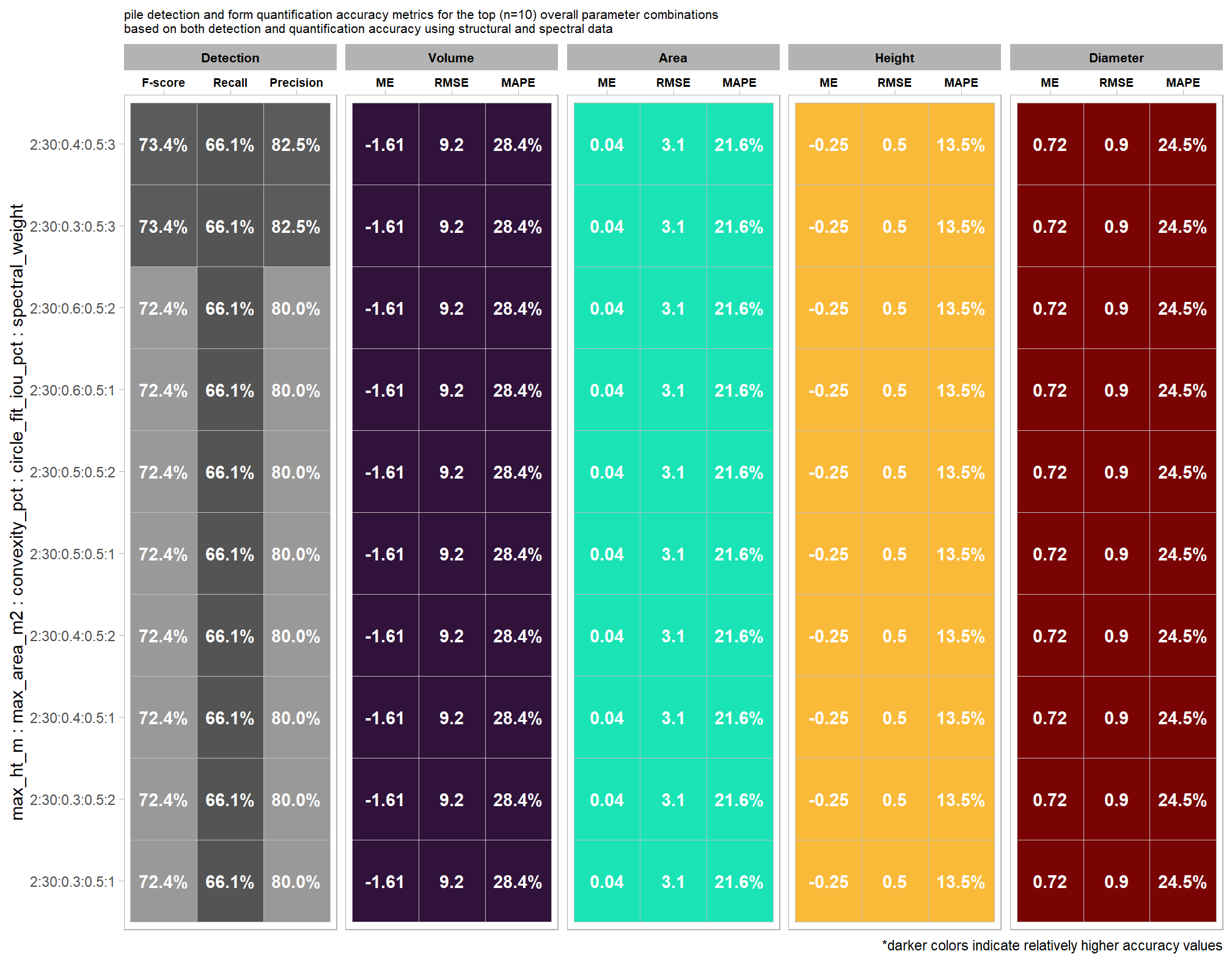
ggplot2::ggsave("../data/bestofthebest_spectral_watersheddetectever.jpg", height = 8.2, width = 10.5)this plot allows for a simultaneous comparison of all metrics for pile detection and pile form quantification. it includes only the parameter combinations that achieved the best balanced accuracy, helping users identify the optimal settings by evaluating the trade-offs between detection and form quantification.
let’s table this
param_combos_spectral_gt_agg %>%
  dplyr::ungroup() %>%
  # filter for best of best
  dplyr::inner_join(
    best_pile_detect_spectral_rn %>%
      dplyr::filter(is_top_recall) %>%
      dplyr::select(rn,spectral_weight,lab,rank_overall)
    , by = dplyr::join_by(rn,spectral_weight)
    , relationship = "one-to-one"
  ) %>%
  # first select to arrange eval_metric
  dplyr::select(
    lab
    , max_ht_m,max_area_m2,convexity_pct,circle_fit_iou_pct,spectral_weight
    # detection
    , f_score, recall, precision
    # quantification
    , tidyselect::ends_with("_mean")
    , tidyselect::ends_with("_rmse")
    # , tidyselect::ends_with("_rrmse")
    , tidyselect::ends_with("_mape")
  ) %>%
  # second select to arrange pile_metric
  dplyr::select(
    lab
    , max_ht_m,max_area_m2,convexity_pct,circle_fit_iou_pct,spectral_weight
    # detection
    , f_score, recall, precision
    # quantification
    , c(tidyselect::contains("volume") & !tidyselect::contains("paraboloid"))
    # , tidyselect::contains("paraboloid_volume")
    , tidyselect::contains("area")
    , tidyselect::contains("height")
    , tidyselect::contains("diameter")
  ) %>%
  # names()
  dplyr::mutate(
    dplyr::across(
      .cols = c(f_score, recall, precision, tidyselect::ends_with("_mape"))
      , .fn = ~ scales::percent(.x, accuracy = 1)
    )
    , dplyr::across(
      .cols = c(tidyselect::ends_with("_mean"))
      , .fn = ~ scales::comma(.x, accuracy = 0.01)
    )
    , dplyr::across(
      .cols = c(tidyselect::ends_with("_rmse"))
      , .fn = ~ scales::comma(.x, accuracy = 0.1)
    )
  ) %>%
  dplyr::mutate(blank= "   " ) %>%
  dplyr::relocate(blank, .before = f_score) %>%
  dplyr::arrange(desc(lab)) %>%
  kableExtra::kbl(
    caption = paste0(
       "pile detection and form quantification accuracy metrics for the final recommended parameter settings"
       # , scales::percent(1-pct_rank_th_top,accuracy=1)
       , " (n="
       , scales::comma(sum(best_pile_detect_spectral_rn$is_top_recall,na.rm=T), accuracy = 1)
       , ")"
       , "<br>using structural and spectral data"
      )
    , col.names = c(
      ""
      ,"max_ht_m","max_area_m2","convexity_pct","circle_fit_iou_pct","spectral_weight"
      , "   "
      , "F-score", "Recall", "Precision"
      , rep(c("ME","RMSE","MAPE"), times = 4)
    )
    , escape = F
  ) %>%
  kableExtra::kable_styling(font_size = 11) %>%
  kableExtra::add_header_above(c(
    " "=7
    , "Detection" = 3
    , "Volume" = 3
    , "Area" = 3
    , "Height" = 3
    , "Diameter" = 3
  )) %>%
  kableExtra::column_spec(seq(7,22,by=3), border_right = TRUE, include_thead = TRUE) %>%
  kableExtra::column_spec(
    column = 8:22
    , extra_css = "font-size: 10px;"
    , include_thead = T
  ) %>%
kableExtra::scroll_box(width = "740px") | max_ht_m | max_area_m2 | convexity_pct | circle_fit_iou_pct | spectral_weight | F-score | Recall | Precision | ME | RMSE | MAPE | ME | RMSE | MAPE | ME | RMSE | MAPE | ME | RMSE | MAPE | ||
|---|---|---|---|---|---|---|---|---|---|---|---|---|---|---|---|---|---|---|---|---|---|
| 2:30:0.4:0.5:3 | 2 | 30 | 0.4 | 0.5 | 3 | 73% | 66% | 82% | -1.61 | 9.2 | 28% | 0.04 | 3.1 | 22% | -0.25 | 0.5 | 14% | 0.72 | 0.9 | 24% | |
| 2:30:0.3:0.5:3 | 2 | 30 | 0.3 | 0.5 | 3 | 73% | 66% | 82% | -1.61 | 9.2 | 28% | 0.04 | 3.1 | 22% | -0.25 | 0.5 | 14% | 0.72 | 0.9 | 24% | |
| 2:30:0.6:0.5:2 | 2 | 30 | 0.6 | 0.5 | 2 | 72% | 66% | 80% | -1.61 | 9.2 | 28% | 0.04 | 3.1 | 22% | -0.25 | 0.5 | 14% | 0.72 | 0.9 | 24% | |
| 2:30:0.6:0.5:1 | 2 | 30 | 0.6 | 0.5 | 1 | 72% | 66% | 80% | -1.61 | 9.2 | 28% | 0.04 | 3.1 | 22% | -0.25 | 0.5 | 14% | 0.72 | 0.9 | 24% | |
| 2:30:0.5:0.5:2 | 2 | 30 | 0.5 | 0.5 | 2 | 72% | 66% | 80% | -1.61 | 9.2 | 28% | 0.04 | 3.1 | 22% | -0.25 | 0.5 | 14% | 0.72 | 0.9 | 24% | |
| 2:30:0.5:0.5:1 | 2 | 30 | 0.5 | 0.5 | 1 | 72% | 66% | 80% | -1.61 | 9.2 | 28% | 0.04 | 3.1 | 22% | -0.25 | 0.5 | 14% | 0.72 | 0.9 | 24% | |
| 2:30:0.4:0.5:2 | 2 | 30 | 0.4 | 0.5 | 2 | 72% | 66% | 80% | -1.61 | 9.2 | 28% | 0.04 | 3.1 | 22% | -0.25 | 0.5 | 14% | 0.72 | 0.9 | 24% | |
| 2:30:0.4:0.5:1 | 2 | 30 | 0.4 | 0.5 | 1 | 72% | 66% | 80% | -1.61 | 9.2 | 28% | 0.04 | 3.1 | 22% | -0.25 | 0.5 | 14% | 0.72 | 0.9 | 24% | |
| 2:30:0.3:0.5:2 | 2 | 30 | 0.3 | 0.5 | 2 | 72% | 66% | 80% | -1.61 | 9.2 | 28% | 0.04 | 3.1 | 22% | -0.25 | 0.5 | 14% | 0.72 | 0.9 | 24% | |
| 2:30:0.3:0.5:1 | 2 | 30 | 0.3 | 0.5 | 1 | 72% | 66% | 80% | -1.61 | 9.2 | 28% | 0.04 | 3.1 | 22% | -0.25 | 0.5 | 14% | 0.72 | 0.9 | 24% |
what is the detection accuracy of these final recommended parameter settings?
# plot it
plt_detection_dist(
  df = param_combos_spectral_gt_agg %>%
    dplyr::ungroup() %>%
    # filter for best of best
    dplyr::inner_join(
      best_pile_detect_spectral_rn %>%
        dplyr::filter(is_top_recall) %>%
        dplyr::distinct(rn,spectral_weight)
      , by = dplyr::join_by(rn,spectral_weight)
      , relationship = "one-to-one"
    )
  , paste0(
       "distribution of pile detection accuracy metrics for the final recommended parameter settings"
       # , scales::percent(1-pct_rank_th_top,accuracy=1)
       , " (n="
       , scales::comma(sum(best_pile_detect_spectral_rn$is_top_recall,na.rm=T), accuracy = 1)
       , ")"
       , "\nusing structural and spectral data"
      )
)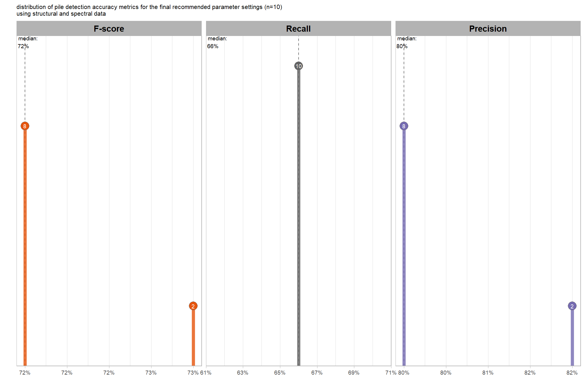
what is the quantification accuracy of these final recommended parameter settings?
# plot it
plt_form_quantification_dist(
  df = param_combos_spectral_gt_agg %>%
    dplyr::ungroup() %>%
    # filter for best of best
    dplyr::inner_join(
      best_pile_detect_spectral_rn %>%
        dplyr::filter(is_top_recall) %>%
        dplyr::distinct(rn,spectral_weight)
      , by = dplyr::join_by(rn,spectral_weight)
      , relationship = "one-to-one"
    )
  , paste0(
       "distribution of pile form quantification accuracy metrics for the final recommended parameter settings"
       # , scales::percent(1-pct_rank_th_top,accuracy=1)
       , " (n="
       , scales::comma(sum(best_pile_detect_spectral_rn$is_top_recall,na.rm=T), accuracy = 1)
       , ")"
       , "\nusing structural and spectral data"
      )
)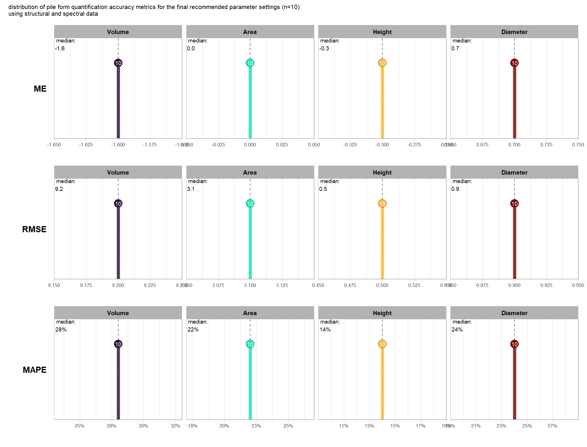
if we look at only these final recommended parameter settings, what is the distribution of individual parameter settings?
pal_param <- viridis::plasma(n=5, begin = 0.1, end = 0.9, alpha = 0.8)
# plot
param_combos_spectral_gt_agg %>%
  dplyr::ungroup() %>%
  # filter for best of best
  dplyr::inner_join(
    best_pile_detect_spectral_rn %>%
      dplyr::filter(is_top_recall) %>%
      dplyr::distinct(rn,spectral_weight)
    , by = dplyr::join_by(rn,spectral_weight)
    , relationship = "one-to-one"
  ) %>%
  dplyr::select(tidyselect::contains("f_score"), max_ht_m,max_area_m2,convexity_pct,circle_fit_iou_pct,spectral_weight) %>%
  tidyr::pivot_longer(
    cols = c(max_ht_m,max_area_m2,convexity_pct,circle_fit_iou_pct,spectral_weight)
    , names_to = "metric"
    , values_to = "value"
  ) %>%
  dplyr::count(metric, value) %>%
  dplyr::group_by(metric) %>%
  dplyr::mutate(
    pct=n/sum(n)
    , lab = paste0(scales::percent(pct,accuracy=0.1), "\nn=", scales::comma(n,accuracy=1))
  ) %>%
  ggplot2::ggplot(
    mapping = ggplot2::aes(x = factor(value), y=pct, label=lab, fill = metric)
  ) +
  ggplot2::geom_col(width = 0.6) +
  ggplot2::geom_text(color = "black", size = 2.5, vjust = -0.2) +
  ggplot2::facet_wrap(facets = dplyr::vars(metric), ncol=2, scales = "free_x") +
  ggplot2::scale_y_continuous(
    breaks = seq(0,1,by=0.2)
    , labels = scales::percent
    , expand = ggplot2::expansion(mult = c(0,0.2))
  ) +
  ggplot2::scale_fill_manual(values = pal_param) +
  ggplot2::labs(
    x = "parameter setting", y = ""
    , fill = ""
    , subtitle = paste0(
       "parameter settings for the final recommended parameter settings"
       # , scales::percent(1-pct_rank_th_top,accuracy=1)
       , " (n="
       , scales::comma(sum(best_pile_detect_spectral_rn$is_top_recall,na.rm=T), accuracy = 1)
       , ")"
       , "\nusing structural and spectral data"
      )
  ) +
  ggplot2::theme_light() +
  ggplot2::theme(
    legend.position = "none"
    , strip.text = ggplot2::element_text(size = 11, color = "black", face = "bold")
    , axis.text.y = ggplot2::element_text(size = 6)
    , axis.text.x = ggplot2::element_text(size = 8)
    , plot.subtitle = ggplot2::element_text(size = 8)
  )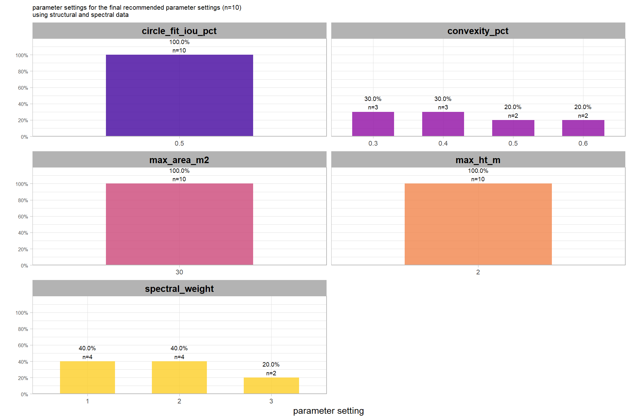
8.5 Final recommended settings: data fusion versus structural only
let’s determine the impact of including both structural and spectral data in a data fusion approach versus using structural data alone (i.e. point cloud or raster data) for detecting and determining the form of slash piles. we’ll do this by comparing only the top 10 final recommended settings which were determined by selecting those sets that not only balance detection and quantification accuracy, but also achieve the highest recall rates. if a parameter combination set using our data fusion approach was selected that did not utilize any spectral data was selected, then it will be dropped from consideration within the data fusion grouping.
we’ll average across all 10 final recommended settings of the data fusion and structural-only approach to determine the impact of including spectral data
first, we need to compile data from the recommended settings from both methods
param_combos_gt_meth_comp <-
  # structural only
  param_combos_gt_agg %>%
  # filter for best of best
  dplyr::inner_join(
    best_pile_detect_rn %>%
      dplyr::filter(is_top_recall) %>%
      dplyr::arrange(rank_overall) %>%
      dplyr::filter(dplyr::row_number()<=10) %>%
      dplyr::distinct(rn)
    , by = "rn"
  ) %>%
  dplyr::mutate(spectral_weight = 0) %>%
# structural+spectral
  dplyr::bind_rows(
    param_combos_spectral_gt_agg %>%
      dplyr::ungroup() %>%
      # filter for best of best
      dplyr::inner_join(
        best_pile_detect_spectral_rn %>%
          dplyr::filter(is_top_recall) %>%
          dplyr::arrange(rank_overall) %>%
          dplyr::filter(dplyr::row_number()<=10) %>%
          dplyr::distinct(rn,spectral_weight)
        , by = dplyr::join_by(rn,spectral_weight)
        , relationship = "one-to-one"
      ) %>%
      # remove non spectral
      dplyr::filter(spectral_weight!=0) %>%
      dplyr::select(names(param_combos_gt_agg),spectral_weight)
  ) %>%
  # make dichotomous factor
  dplyr::mutate(
    spectral_weight_fact = ifelse(spectral_weight==0,"structural only","structural+spectral") %>%
      factor()
  )
let’s look at the distributions of the evaluation metrics
df_temp <-
  param_combos_gt_meth_comp %>%
  dplyr::select(
    max_ht_m,max_area_m2,convexity_pct,circle_fit_iou_pct,spectral_weight
    , spectral_weight_fact
    # detection
    , f_score, recall, precision
    # quantification
    , tidyselect::ends_with("_rmse")
    , tidyselect::ends_with("_rrmse")
    , tidyselect::ends_with("_mean")
    , tidyselect::ends_with("_mape")
  ) %>%
  tidyr::pivot_longer(
    cols = c(
      f_score, recall, precision
      , tidyselect::ends_with("_rmse")
      , tidyselect::ends_with("_rrmse")
      , tidyselect::ends_with("_mean")
      , tidyselect::ends_with("_mape")
    )
    , names_to = "metric"
    , values_to = "value"
  ) %>%
  dplyr::mutate(
    eval_metric = stringr::str_extract(metric, "(_rmse|_rrmse|_mean|_mape|f_score|recall|precision)$") %>%
      stringr::str_remove_all("_") %>%
      stringr::str_replace_all("mean","me") %>%
      toupper() %>%
      factor(
        ordered = T
        , levels = c("FSCORE","RECALL","PRECISION", "ME","RMSE","RRMSE","MAPE")
        , labels = c("F-score","Recall","Precision", "ME","RMSE","RRMSE","MAPE")
      ) %>% forcats::fct_rev()
    , pile_metric = metric %>%
      stringr::str_remove("(_rmse|_rrmse|_mean|_mape)$") %>%
      stringr::str_extract("(paraboloid_volume|volume|area|height|diameter)") %>%
      dplyr::coalesce("detection") %>%
      factor(
        ordered = T
        , levels = c(
          "detection"
          , "volume"
          , "paraboloid_volume"
          , "area"
          , "height"
          , "diameter"
        )
        , labels = c(
          "Detection"
          , "Volume"
          , "Volume paraboloid"
          , "Area"
          , "Height"
          , "Diameter"
        )
      )
    , value_lab = dplyr::case_when(
        eval_metric %in% c("F-score","Recall","Precision", "RRMSE", "MAPE") ~ scales::percent(value,accuracy=0.1)
        , eval_metric == "ME" ~ scales::comma(value,accuracy=0.01)
        , T ~ scales::comma(value,accuracy=0.1)
      )
    , overall_metric = forcats::fct_cross(pile_metric,eval_metric)
  ) %>%
  dplyr::ungroup() %>%
  dplyr::filter(eval_metric!="RRMSE")
  # dplyr::count(overall_metric,pile_metric,eval_metric) %>%
  # dplyr::arrange(pile_metric,eval_metric)
  # dplyr::arrange(overall_metric)
# aggregate
xxxdf_temp <- df_temp %>%
  dplyr::group_by(spectral_weight_fact, overall_metric) %>%
  dplyr::summarise(value = median(value,na.rm=T)) %>%
  dplyr::ungroup() %>%
  dplyr::mutate(
    value_lab = paste0(
        "median:\n"
      , dplyr::case_when(
        stringr::str_detect(
          overall_metric
          , "(F-score|Recall|Precision|RRMSE|MAPE)"
        ) ~ scales::percent(value,accuracy=0.1)
        # , eval_metric == "ME" ~ scales::comma(value,accuracy=0.01)
        , T ~ scales::comma(value,accuracy=0.1)
      )
    )
  )
# xxxdf_temp

# plot
df_temp %>%
  ggplot2::ggplot(
      mapping = ggplot2::aes(
        x = value
        , color = spectral_weight_fact, fill = spectral_weight_fact
        , group = spectral_weight_fact
      )
    ) +
    ggplot2::geom_density(color = NA, alpha = 0.7) +
    ggplot2::geom_rug() +
    ggplot2::geom_vline(
      data = xxxdf_temp
      , mapping = ggplot2::aes(xintercept = value, color = spectral_weight_fact)
      , linetype = "dashed", lwd = 1
    ) +
    # ggplot2::geom_text(
    #   data = xxxdf_temp
    #   , mapping = ggplot2::aes(
    #     x = -Inf, y = Inf # always in upper left?
    #     # x = value, y = 0
    #     , label = value_lab
    #   )
    #   , hjust = -0.1, vjust = 1 # always in upper left?
    #   # , hjust = -0.1, vjust = -5
    #   , size = 2.5, color = "black"
    # ) +
    harrypotter::scale_fill_hp_d(option = "hermionegranger") +
    harrypotter::scale_color_hp_d(option = "hermionegranger") +
    ggplot2::facet_wrap(facets = dplyr::vars(overall_metric), ncol = 4, scales = "free") +
    ggplot2::labs(
      x = "", y = ""
      , subtitle = "", fill = "", color = ""
      , caption = "*median value represented by dashed line"
    ) +
    ggplot2::theme_light() +
    ggplot2::theme(
      legend.position = "top"
      , strip.text = ggplot2::element_text(size = 9, color = "black", face = "bold")
      , axis.text.x = ggplot2::element_text(size = 7)
      , axis.text.y = ggplot2::element_blank()
      , plot.subtitle = ggplot2::element_text(size = 8)
    ) +
    ggplot2::guides(
      color = "none"
    )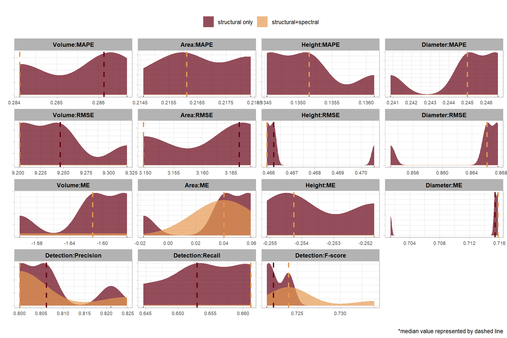
for the most part, including the spectral data for slash pile detection does not alter the quantification of slash pile form when using these optimal parameter settings. this is because spectral information is used solely to filter candidate piles, meaning it neither reshapes existing ones nor introduces new detections.
however, including the spectral data does appear to significantly alter slash pile detection accuracy as measured by F-score primarily by increasing the precision of the detection method by using the spectral data to filter out false positive (commission) predictions which would have been kept as predictions when using only the structural data
let’s do some statistical quantification of the impact of including the spectral data
we can use the marginaleffects package to compare and contrast the mean estimates by group. this approach calculates the average difference in the predicted outcome (evaluation metric in our case) between the different levels of the factor variable (structural only versus structural+spectral data). this is similar to the Tukey’s Honestly Significant Difference (HSD) test to compare group means to determine if there are significant differences between them.
# quick mod
dep_vars_temp <- # c("f_score","recall","precision")
  param_combos_gt_meth_comp %>%
  dplyr::select(
    # detection
    f_score, recall, precision
    # quantification
    , tidyselect::ends_with("_rmse")
    # , tidyselect::ends_with("_rrmse")
    , tidyselect::ends_with("_mean")
    , tidyselect::ends_with("_mape")
  ) %>%
  names()
# list of formulas
formulas_temp <- dep_vars_temp %>%
  purrr::map(~stats::reformulate(c("spectral_weight_fact","-1"), response = .x))
names(formulas_temp) <- dep_vars_temp
# formulas_temp
models_temp <- formulas_temp %>%
  purrr::map(\(x) lm(formula = x, data = param_combos_gt_meth_comp))
names(models_temp) <- dep_vars_temp
# models_temp

## comparisons
# purrr::map_df(models_temp, broom::tidy, .id = "metric")
pred_df_temp <- models_temp %>%
  purrr::map_df(
    \(x)
    marginaleffects::avg_comparisons(
      model = x
      , variables = list(spectral_weight_fact = "pairwise")
        # list(spectral_weight_fact = "revpairwise")
      , comparison = "difference"
    )
    , .id = "metric"
  ) %>%
  dplyr::mutate(
    contrast = contrast %>%
      stringr::str_remove_all("mean\\(") %>%
      stringr::str_remove_all("\\)")
    , sig_lvl = dplyr::case_when(
        p.value <= 0.01 ~ "0.01"
        , p.value <= 0.05 ~ "0.05"
        , p.value <= 0.1 ~ "0.10"
        , T ~ "not significant"
      ) %>%
      factor(
        ordered = T
        , levels = c(
          "0.01"
          , "0.05"
          , "0.10"
          , "not significant"
        )
      )
    # pretty metric
    , eval_metric = stringr::str_extract(metric, "(_rmse|_rrmse|_mean|_mape)$") %>%
      stringr::str_remove_all("_") %>%
      stringr::str_replace_all("mean","me") %>%
      dplyr::coalesce("detection") %>%
      toupper() %>%
      factor(
        ordered = T
        , levels = c("DETECTION", "ME","RMSE","RRMSE","MAPE")
        , labels = c("Detection", "ME","RMSE","RRMSE","MAPE")
      ) %>% forcats::fct_rev()
    , pile_metric = metric %>%
      stringr::str_remove("(_rmse|_rrmse|_mean|_mape)$") %>%
      stringr::str_extract("(paraboloid_volume|volume|area|height|diameter|f_score|recall|precision)") %>%
      factor(
        ordered = T
        , levels = c(
          "f_score","recall","precision"
          , "volume"
          , "paraboloid_volume"
          , "area"
          , "height"
          , "diameter"
        )
        , labels = c(
          "F-score","Recall","Precision"
          , "Volume"
          , "Volume paraboloid"
          , "Area"
          , "Height"
          , "Diameter"
        )
      )
    , value_lab = dplyr::case_when(
        eval_metric %in% c("Detection", "F-score","Recall","Precision", "RRMSE", "MAPE") ~ scales::percent(estimate,accuracy=0.1)
        , eval_metric == "ME" ~ scales::comma(estimate,accuracy=0.01)
        , T ~ scales::comma(estimate,accuracy=0.1)
      )
  )
# pred_df_temp %>% dplyr::glimpse()
# plot
pred_df_temp %>%
  # plot
  ggplot2::ggplot(mapping = ggplot2::aes(x = estimate, y = pile_metric, color = sig_lvl)) +
    ggplot2::geom_vline(xintercept = 0, linetype = "dashed", color = "gray44") +
    ggplot2::geom_linerange(
      mapping = ggplot2::aes(xmin = conf.low, xmax = conf.high)
      , linewidth = 2
    ) +
    ggplot2::geom_point(size = 3) +
    ggplot2::geom_text(mapping = ggplot2::aes(label = value_lab), color = "black", vjust = 1.5) +
    ggplot2::annotate(
      "text", x = -Inf, y = Inf
      , label = stringr::str_replace_all(pred_df_temp$contrast[1]," - "," < ") # "Top Left Text"
      , hjust = 0, vjust = 1
      , size = 2.5
    ) +
    ggplot2::annotate(
      "text", x = Inf, y = Inf
      , label = stringr::str_replace_all(pred_df_temp$contrast[1]," - "," > ") # "Top Right Text"
      , hjust = 1, vjust = 1
      , size = 2.5
    ) +
    ggplot2::scale_color_viridis_d(option = "mako", begin = 0.2, end = 0.8, drop = F) +
    ggplot2::facet_wrap(facets = dplyr::vars(eval_metric), scales = "free") +
    ggplot2::scale_x_continuous(labels = 0, breaks = 0, expand = expansion(mult = c(0.8, 0.7))) +
    ggplot2::labs(
      y = ""
      , x = paste0("Difference: ", pred_df_temp$contrast[1])
      , subtitle = "Mean group constrasts"
      , color = "sig. level"
    ) +
    theme_light() +
    theme(
      legend.position = "bottom"
      , strip.text = ggplot2::element_text(size = 11, color = "black", face = "bold")
      , axis.text.y = ggplot2::element_text(size = 10, color = "black", face = "bold")
      , axis.text.x = ggplot2::element_text(size = 10, color = "black")
      # , axis.ticks.x = ggplot2::element_blank()
      , panel.grid.major.x = ggplot2::element_blank()
      , panel.grid.minor.x = ggplot2::element_blank()
      , plot.subtitle = ggplot2::element_text(size = 8)
    )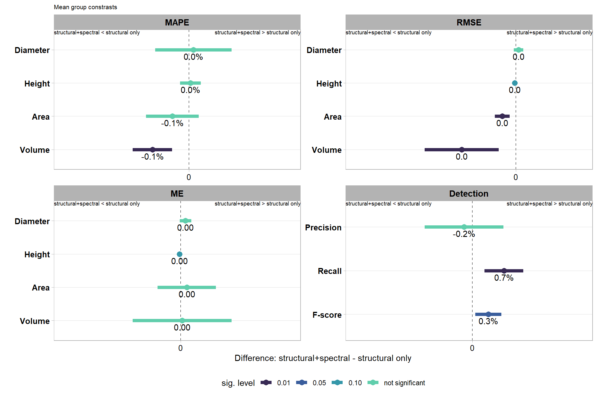
and view the contrasts in a table