Section 2 Data Processing
Load the standard libraries we use to do work
# bread-and-butter
library(tidyverse) # the tidyverse
library(viridis) # viridis colors
library(harrypotter) # hp colors
library(RColorBrewer) # brewer colors
library(scales) # work with number and plot scales
library(latex2exp)

# visualization
library(mapview) # interactive html maps
library(kableExtra) # tables
library(patchwork) # combine plots
library(corrplot) # correlation plots

# spatial analysis
library(terra) # raster
library(sf) # simple features
library(lidR) # lidar data
library(rgl) # 3d plots
library(cloud2trees) # the cloud2trees
library(glcm) # textures of rasters

# modelling
library(brms)
library(tidybayes)
2.1 Slash Pile Vector Data
Slash pile field measurements were taken by measuring the height and diameter (longest side of pile) using a laser hypsometer
For volume estimation, we’ll model the ground truth slash piles as a paraboloid, specifically a parabolic dome, assuming a perfectly circular base and sides curved smoothly to a peak. Assuming a paraboloid shape is common for quantifying slash pile volume (Hardy 1996; Long & Boston 2014) and may better represent the diverse shapes of real-world slash piles than assuming a conical or half-sphere form. A paraboloid can represent a variety of shapes including those that are taller and more conical, or flatter and more spread out, because it allows the measured height and width to influence the volume calculation independently. This makes the paraboloid potentially more robust for estimating volumes of piles with varying aspect ratios.
the volume formula for a paraboloid is:
\[ V = \frac{1}{8}\pi \cdot width^2 \cdot height \]
# points recorded in field
slash_piles_points <- sf::st_read(
    "../data/PFDP_Data/PFDP_SlashPiles/SlashPiles.shp"
    # "f:\\PFDP_Data\\PFDP_SlashPiles\\SlashPiles.shp"
  ) %>%
  dplyr::rename_with(tolower)
## Reading layer `SlashPiles' from data source
## `C:\Data\usfs\manitou_slash_piles\data\PFDP_Data\PFDP_SlashPiles\SlashPiles.shp'
## using driver `ESRI Shapefile'
## Simple feature collection with 122 features and 8 fields
## Geometry type: POINT
## Dimension: XYZM
## Bounding box: xmin: 1019067 ymin: 4334804 xmax: 1019496 ymax: 4335198
## z_range: zmin: 0 zmax: 2831.171
## m_range: mmin: 0 mmax: 1566318000
## Projected CRS: WGS 84 / UTM zone 12N# polygons annotated using RGB and field-collected points
slash_piles_polys <- sf::st_read(
"../data/PFDP_Data/PFDP_SlashPiles/SlashPiles_Polygons.shp"
# "f:\\PFDP_Data\\PFDP_SlashPiles\\SlashPiles_Polygons.shp"
) %>%
dplyr::rename_with(tolower) %>%
dplyr::mutate(pile_id = as.factor(pile_idx)) %>%
dplyr::select(-pile_idx) %>%
sf::st_make_valid() %>%
dplyr::filter(sf::st_is_valid(.)) %>%
# add point data to polygon
sf::st_join(slash_piles_points %>% sf::st_zm()) %>%
# fix multipolygons
dplyr::ungroup() %>%
dplyr::mutate(treeID = dplyr::row_number()) %>%
cloud2trees::simplify_multipolygon_crowns() %>%
dplyr::select(-treeID) %>%
# calculate area and volume
dplyr::mutate(
# height
height_m = height*0.3048
, field_diameter_m = diameter*0.3048 # *0.3048 or /3.281 to convert to m
, field_radius_m = (diameter/2)*0.3048 # *0.3048 or /3.281 to convert to m
, image_gt_area_m2 = sf::st_area(.) %>% as.numeric()
, field_gt_area_m2 = pi*field_radius_m^2
# volume
, image_gt_volume_m3 = (1/8) * pi * ( (sqrt(image_gt_area_m2/pi)*2)^2 ) * height_m # (1/8) * pi * (shape_length^2) * max_height_m
# (sqrt(image_gt_area_m2/pi)*2) = diameter assuming of circle covering same area
, field_gt_volume_m3 = (1/8) * pi * (field_diameter_m^2) * height_m # (1/8) * pi * (shape_length^2) * max_height_m
)## Reading layer `SlashPiles_Polygons' from data source
## `C:\Data\usfs\manitou_slash_piles\data\PFDP_Data\PFDP_SlashPiles\SlashPiles_Polygons.shp'
## using driver `ESRI Shapefile'## Simple feature collection with 183 features and 1 field
## Geometry type: POLYGON
## Dimension: XY
## Bounding box: xmin: 1018968 ymin: 4334777 xmax: 1019547 ymax: 4335271
## Projected CRS: WGS 84 / UTM zone 12N# stand boundary?
stand_boundary <- sf::st_read("../data/PFDP_Data/Tree_Data/GIS/PFDP_Boundary.shp") %>%
sf::st_transform(sf::st_crs(slash_piles_polys))## Reading layer `PFDP_Boundary' from data source
## `C:\Data\usfs\manitou_slash_piles\data\PFDP_Data\Tree_Data\GIS\PFDP_Boundary.shp'
## using driver `ESRI Shapefile'
## Simple feature collection with 1 feature and 16 fields
## Geometry type: POLYGON
## Dimension: XY
## Bounding box: xmin: 1019059 ymin: 4334795 xmax: 1019520 ymax: 4335217
## Projected CRS: NAD83 / UTM zone 12N# add in/out to piles data
slash_piles_polys <- slash_piles_polys %>%
dplyr::mutate(
is_in_stand = pile_id %in% (slash_piles_polys %>%
sf::st_intersection(stand_boundary) %>%
sf::st_drop_geometry() %>%
dplyr::pull(pile_id))
)what?
## Rows: 183
## Columns: 18
## $ pile_id            <fct> 1, 2, 3, 4, 5, 6, 7, 8, 9, 10, 11, 12, 13, 14, 15, …
## $ objectid           <dbl> 112, 111, 115, 110, 108, 109, 113, 114, 107, 104, N…
## $ comment            <chr> "Hand Pile", "Hand Pile", "Hand Pile", "Hand Pile",…
## $ comment2           <chr> NA, NA, NA, NA, NA, NA, NA, NA, NA, NA, NA, NA, NA,…
## $ height             <dbl> 6.0, 7.0, 7.0, 6.5, 6.0, 6.5, 7.5, 6.0, 6.5, 8.0, 7…
## $ diameter           <dbl> 10.0, 10.8, 10.0, 9.5, 8.0, 9.5, 10.0, 11.3, 10.0, …
## $ xcoord             <dbl> 1019292, 1019290, 1019330, 1019277, 1019264, 101927…
## $ ycoord             <dbl> 4335145, 4335158, 4335168, 4335149, 4335111, 433512…
## $ refcorner          <chr> "R17", "R18", "T18", "Q18", "Q16", "Q16", "R17", "S…
## $ geometry           <POLYGON [m]> POLYGON ((1019292 4335147, ..., POLYGON ((1…
## $ height_m           <dbl> 1.8288, 2.1336, 2.1336, 1.9812, 1.8288, 1.9812, 2.2…
## $ field_diameter_m   <dbl> 3.04800, 3.29184, 3.04800, 2.89560, 2.43840, 2.8956…
## $ field_radius_m     <dbl> 1.52400, 1.64592, 1.52400, 1.44780, 1.21920, 1.4478…
## $ image_gt_area_m2   <dbl> 9.167566, 9.151451, 8.202037, 11.700286, 8.130412, …
## $ field_gt_area_m2   <dbl> 7.296588, 8.510740, 7.296588, 6.585170, 4.669816, 6…
## $ image_gt_volume_m3 <dbl> 8.382822, 9.762768, 8.749933, 11.590304, 7.434449, …
## $ field_gt_volume_m3 <dbl> 6.672000, 9.079257, 7.784000, 6.523270, 4.270080, 6…
## $ is_in_stand        <lgl> TRUE, TRUE, TRUE, TRUE, TRUE, TRUE, TRUE, TRUE, TRU…
where?
# mapview::mapview(slash_piles_points, zcol = "comment", layer.name = "slash piles")
mapview::mapview(
  stand_boundary
  , color = "black"
  , lwd = 1
  , alpha.regions = 0
  , label = FALSE
  , legend = FALSE
  , popup = FALSE
  , layer.name = "stand boundary"
) +
mapview::mapview(slash_piles_polys, zcol = "is_in_stand", layer.name = "'in' slash piles")
let’s check the field-collected and image-annotated measurements of volume and area. for both volume measurements, a paraboloid geometry is assumed for calculation with the image-annotated volume relying on the field-collected heights
p1_temp <- slash_piles_polys %>%
  ggplot2::ggplot(mapping = ggplot2::aes(x = image_gt_area_m2, y =field_gt_area_m2)) +
  ggplot2::geom_abline(lwd = 1.5) +
  ggplot2::geom_point(ggplot2::aes(color = height)) +
  ggplot2::geom_smooth(method = "lm", se=F, color = "tomato", linetype = "dashed") +
  ggplot2::scale_color_viridis_c(option = "mako", direction = -1, alpha = 0.8) +
  ggplot2::scale_x_continuous(limits = c(0,85)) +
  ggplot2::scale_y_continuous(limits = c(0,85)) +
  ggplot2::labs(
    x = "image-annotated area (m2)", y = "field-collected area (m2)"
    , color = "height (m)"
    , subtitle = "area (m2) comparison"
  ) +
  ggplot2::theme_light()
p2_temp <-
  slash_piles_polys %>%
  ggplot2::ggplot(mapping = ggplot2::aes(x = image_gt_volume_m3, y =field_gt_volume_m3)) +
  ggplot2::geom_abline(lwd = 1.5) +
  ggplot2::geom_point(ggplot2::aes(color = height)) +
  ggplot2::geom_smooth(method = "lm", se=F, color = "tomato", linetype = "dashed") +
  ggplot2::scale_color_viridis_c(option = "mako", direction = -1, alpha = 0.8) +
  ggplot2::scale_x_continuous(limits = c(0,225)) +
  ggplot2::scale_y_continuous(limits = c(0,225)) +
  ggplot2::labs(
    x = "image-annotated volume (m3)", y = "field-collected volume (m3)"
    , color = "height (m)"
    , subtitle = "volume (m3) comparison"
  ) +
  ggplot2::theme_light()
patchwork::wrap_plots(list(p1_temp,p2_temp), guides = "collect") &
  ggplot2::theme(legend.position = "bottom")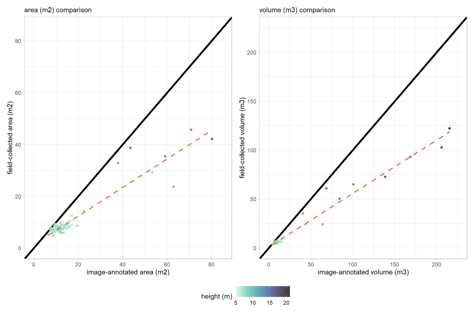
image-annotated values are consistently larger than field-collected values. this indicates a systematic bias in either the image annotation or field collection process (or both) leading to a misalignment of measurements
quick summary of these measurements
slash_piles_polys %>%
  sf::st_drop_geometry() %>%
  dplyr::select(height_m, tidyselect::ends_with("area_m2"), tidyselect::ends_with("volume_m3")) %>%
  summary()
## height_m image_gt_area_m2 field_gt_area_m2 image_gt_volume_m3
## Min. :1.524 Min. : 6.560 Min. : 4.670 Min. : 6.498
## 1st Qu.:1.829 1st Qu.: 9.678 1st Qu.: 6.690 1st Qu.: 9.732
## Median :1.981 Median : 11.779 Median : 7.591 Median : 11.572
## Mean :2.182 Mean : 19.085 Mean :10.608 Mean : 25.268
## 3rd Qu.:2.134 3rd Qu.: 14.262 3rd Qu.: 8.829 3rd Qu.: 14.110
## Max. :6.401 Max. :114.675 Max. :63.069 Max. :323.198
## NA's :67 NA's :67 NA's :67
## field_gt_volume_m3
## Min. : 4.270
## 1st Qu.: 6.650
## Median : 7.523
## Mean : 15.284
## 3rd Qu.: 8.761
## Max. :183.080
## NA's :672.2 Load RGB orthomosaic rasters
Orthomosaic tif files from the UAS flight imagery that were created in Agisoft Metashape are loaded and stitched together via terra::mosaic.
  # read list of orthos
  ortho_list_temp <- list.files(
    "f:\\PFDP_Data\\p4pro_images\\P4Pro_06_17_2021_half_half_optimal\\3_dsm_ortho\\2_mosaic"
    , pattern = "*\\.(tif|tiff)$", full.names = T)[] %>%
    purrr::map(function(x){terra::rast(x)})

  ortho_list_temp[[1]] %>% terra::res()
  #   terra::aggregate(20) %>%
  #   terra::plotRGB(r = 1, g = 2, b = 3, stretch = "hist", colNA = "transparent")

  ####### ensure the resolution of the rasters matches
    # terra::res(ortho_list_temp[[1]])

    ## function
    change_res_fn <- function(r, my_res=1, m = "bilinear"){
      r2 <- r
      terra::res(r2) <- my_res
      r2 <- terra::resample(r, r2, method = m)
      return(r2)
    }
    ## apply the function
    ortho_list_temp <- 1:length(ortho_list_temp) %>%
      purrr::map(function(x){change_res_fn(ortho_list_temp[[x]], my_res=0.15)})

    # terra::res(ortho_list_temp[[1]])

    # ortho_list_temp[[1]] %>%
    #   terra::aggregate(2) %>%
    #   terra::plotRGB(r = 1, g = 2, b = 3, stretch = "hist", colNA = "transparent")

  ######## mosaic the raster list
    ortho_rast <- terra::mosaic(
      terra::sprc(ortho_list_temp)
      , fun = "min" # min only thing that works
    )

    names(ortho_rast) <- c("red","green","blue","alpha")

  # ortho_rast %>%
  #   terra::aggregate(4) %>%
  #   terra::plotRGB(r = 1, g = 2, b = 3, stretch = "lin", colNA = "transparent")
ortho plot fn
######################################################################################
# function to plot ortho + stand
######################################################################################
ortho_plt_fn = function(stand = las_ctg_dta %>% sf::st_union() %>% sf::st_as_sf(), buffer = 20){
# convert to stars
  ortho_st <- ortho_rast %>%
    terra::subset(subset = c(1,2,3)) %>%
    terra::crop(
      stand %>% sf::st_buffer(buffer) %>% terra::vect()
    ) %>%
    # terra::aggregate(fact = 2, fun = "mean", na.rm = T) %>%
    stars::st_as_stars()

  # convert to rgb
  ortho_rgb <- stars::st_rgb(
    ortho_st[,,,1:3]
    , dimension = 3
    , use_alpha = FALSE
    # , stretch = "histogram"
    , probs = c(0.005, 0.995)
    , stretch = "percent"
  )
  # ggplot
  plt_rgb <- ggplot2::ggplot() +
    stars::geom_stars(data = ortho_rgb[]) +
    ggplot2::scale_fill_identity(na.value = "transparent") + # !!! don't take this out or RGB plot will kill your computer
    ggplot2::scale_x_continuous(expand = c(0, 0)) +
    ggplot2::scale_y_continuous(expand = c(0, 0)) +
    ggplot2::labs(
      x = ""
      , y = ""
    ) +
    ggplot2::theme_void()

  # return(plt_rgb)
  # combine all plot elements
  plt_combine = plt_rgb +
    # geom_sf(
    #   data = stand
    #   , alpha = 0
    #   , lwd = 1.5
    #   , color = "gray22"
    # ) +
    ggplot2::theme(
      legend.position = "top" # c(0.5,1)
      , legend.direction = "horizontal"
      , legend.margin = ggplot2::margin(0,0,0,0)
      , legend.text = ggplot2::element_text(size = 8)
      , legend.title = ggplot2::element_text(size = 8)
      , legend.key = ggplot2::element_rect(fill = "white")
      # , plot.title = ggtext::element_markdown(size = 10, hjust = 0.5)
      , plot.title = ggplot2::element_text(size = 8, hjust = 0.5, face = "bold")
      , plot.subtitle = ggplot2::element_text(size = 6, hjust = 0.5, face = "italic")
    )
  return(plt_combine)
}
plot an example slash pile RGB image
stand_temp = slash_piles_points %>%
    dplyr::filter(tolower(comment)=="mechanical pile") %>%
    dplyr::arrange(desc(diameter)) %>%
    dplyr::slice(1) %>%
    sf::st_zm() %>%
    sf::st_buffer(10, endCapStyle = "SQUARE") %>%
    sf::st_transform(terra::crs(ortho_rast))
# check it with the ortho
ortho_plt_fn(stand = stand_temp)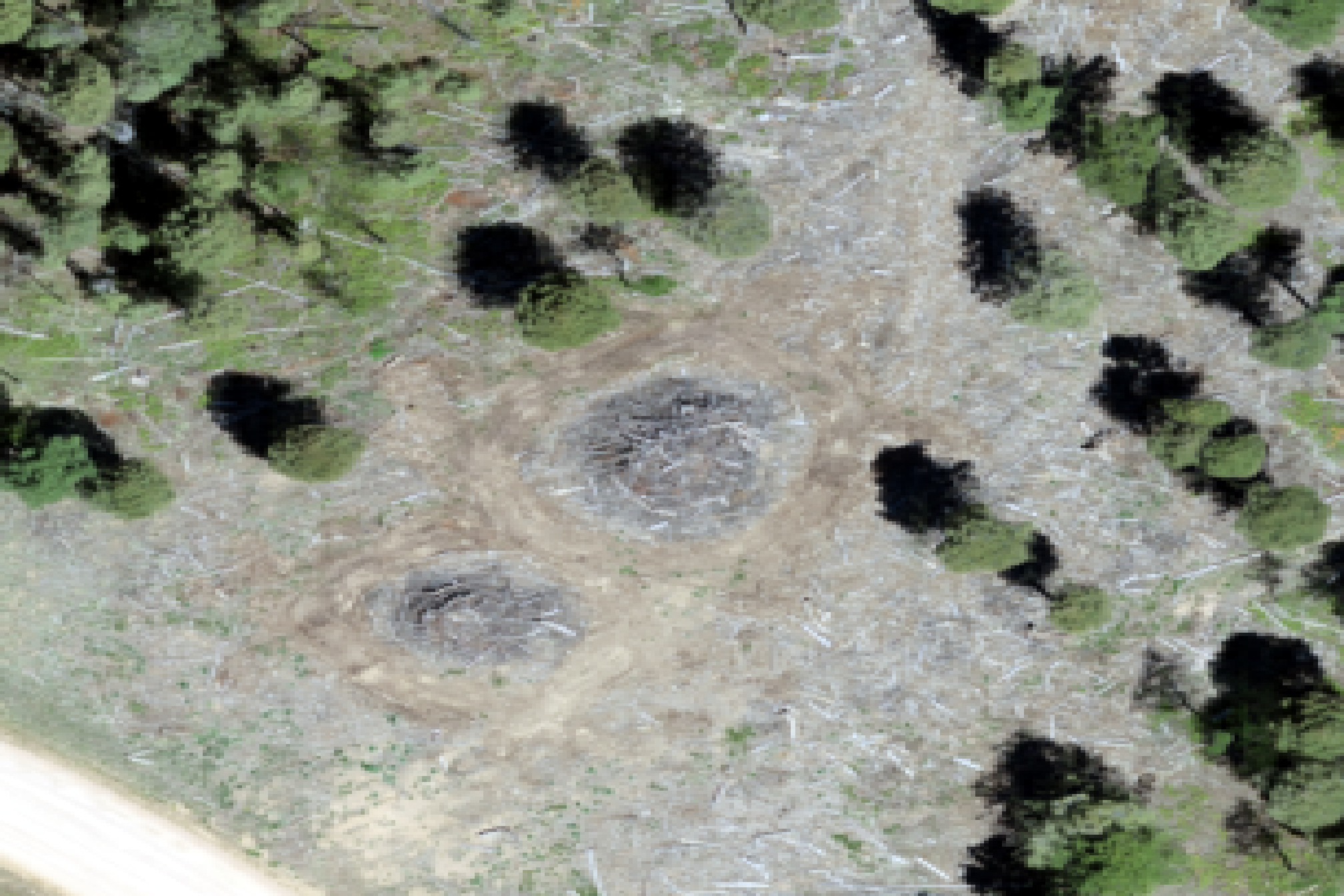
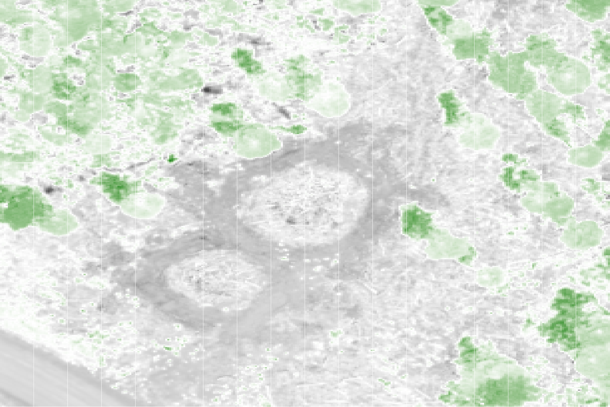
2.2.1 Example ratio-based index
let’s define a general function for a ratio based (vegetation) index
spectral_index_fn <- function(rast, layer1, layer2) {
  bk <- rast[[layer1]]
  bi <- rast[[layer2]]
  vi <- (bk - bi) / (bk + bi)
  return(vi)
}
The Green-Red Vegetation Index (GRVI) uses the reflectance of green and red bands to assess vegetation health and identify ground cover types. The formula is GRVI = (green - red) / (green + red). Higher GRVI values indicate healthy vegetation, while negative values suggest soils, and values near zero may indicate water or snow.
grvi_rast <- spectral_index_fn(rast = ortho_rast, layer1 = 2, layer2 = 1)
names(grvi_rast) <- c("grvi")
terra::plot(grvi_rast, col = harrypotter::hp(n=100, option = "Slytherin"))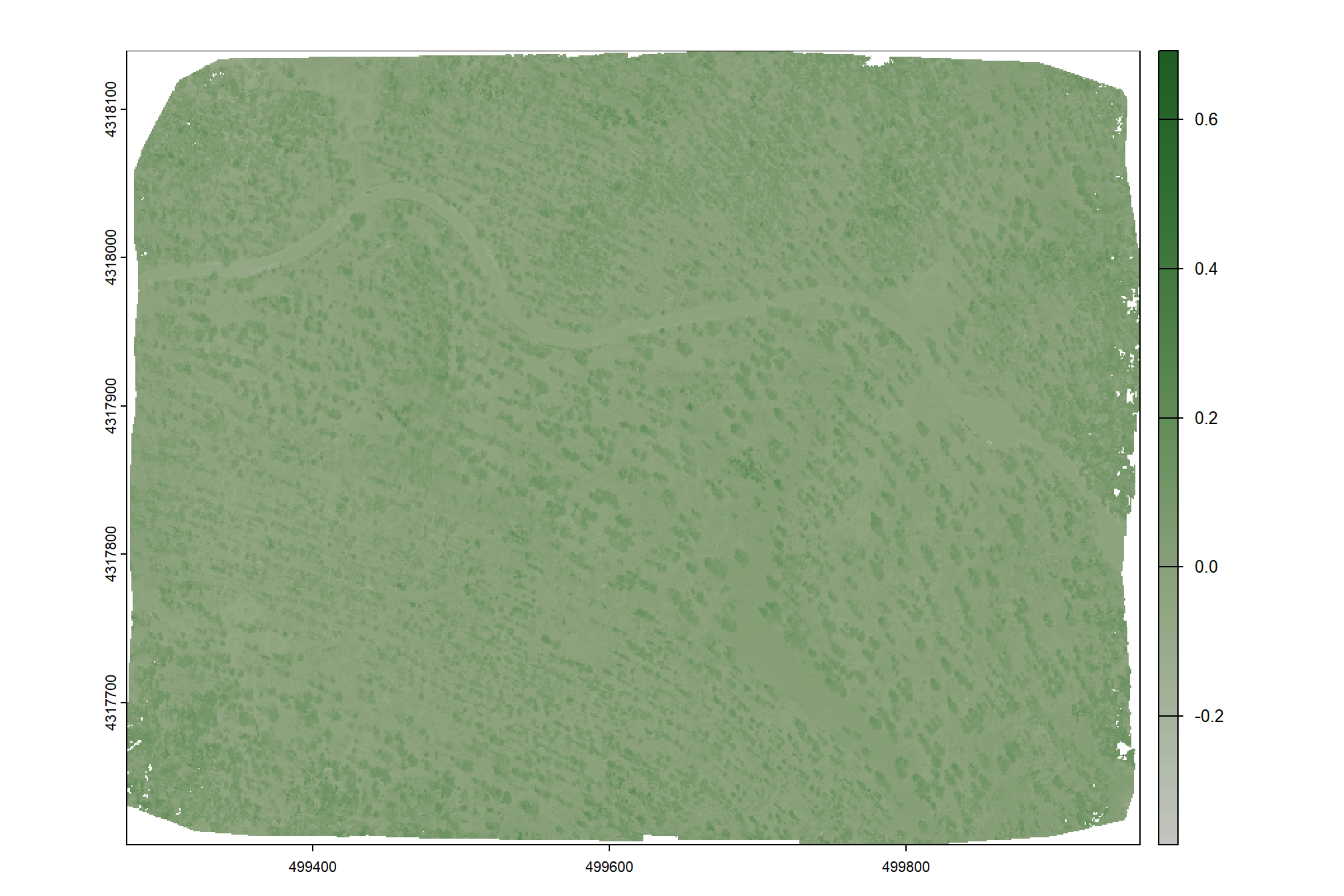
let’s check the GRVI for a pile
# check it with the ortho
grvi_rast %>%
  terra::crop(stand_temp %>% sf::st_buffer(20)) %>%
  terra::as.data.frame(xy=T) %>%
  dplyr::rename(f=3) %>%
  ggplot2::ggplot() +
  ggplot2::geom_tile(ggplot2::aes(x=x,y=y,fill = f), color = NA) +
  ggplot2::labs(fill="CHM (m)") +
  # harrypotter::scale_fill_hp("slytherin") +
  scale_fill_gradient2(low = "black", high = "forestgreen") +
  scale_x_continuous(expand = c(0, 0)) +
  scale_y_continuous(expand = c(0, 0)) +
  ggplot2::theme_void() +
  theme(
      legend.position = "none" # c(0.5,1)
      , legend.direction = "horizontal"
      , legend.margin = margin(0,0,0,0)
      , legend.text = element_text(size = 8)
      , legend.title = element_text(size = 8)
      , legend.key = element_rect(fill = "white")
      # , plot.title = ggtext::element_markdown(size = 10, hjust = 0.5)
      , plot.title = element_text(size = 10, hjust = 0.5, face = "bold")
      , plot.subtitle = element_text(size = 8, hjust = 0.5, face = "italic")
    )
2.3 Study area imagery
let’s look at the RGB imagery and pile locations
# get the base plot
plt_rgb_ortho <- ortho_plt_fn(
  slash_piles_points %>%
  sf::st_bbox() %>%
  sf::st_as_sfc() %>%
  sf::st_buffer(50) %>%
  sf::st_transform(terra::crs(ortho_rast))
)
# add pile locations
plt_rgb_ortho +
  ggplot2::geom_sf(
    data = slash_piles_points %>% sf::st_transform(terra::crs(ortho_rast))
    , ggplot2::aes() # size = diameter
    , shape = 1
    , color = "firebrick"
  ) +
  ggplot2::theme(legend.position = "none")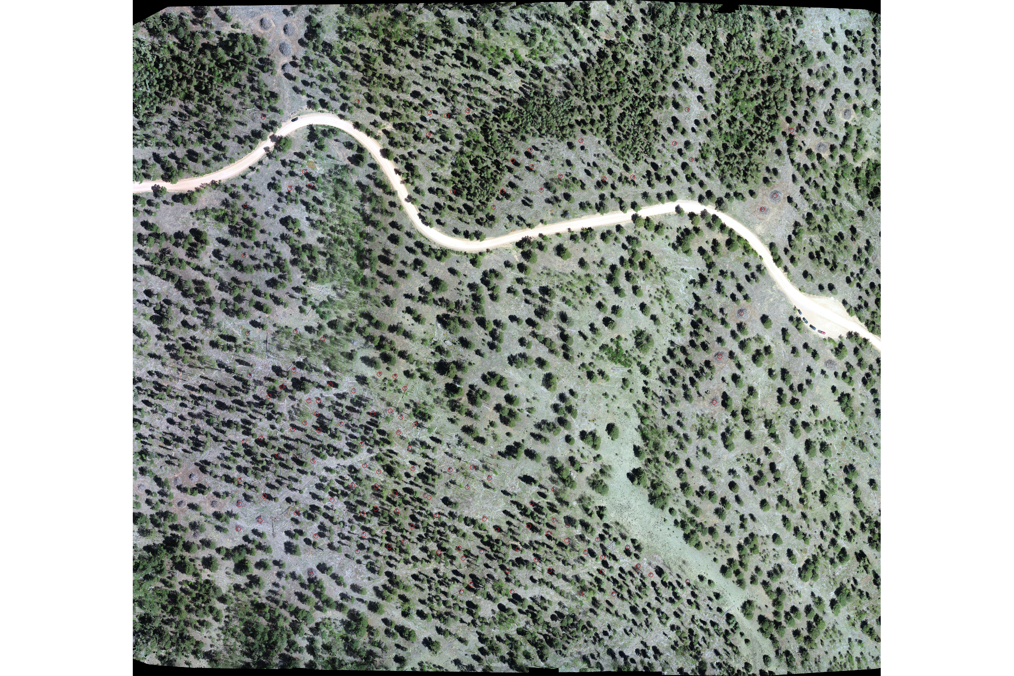
notice these are point measurements of plot locations and the points are not precisely in the center of the pile. notice also there are piles in the imagery that were not measured (e.g. upper-left corner)
Update: we created image-annotated pile polygons using the RBG and field-collected pile location data
let’s make a panel of plots for each pile
p_fn_temp <- function(
    rn
    , df = slash_piles_polys %>% dplyr::filter(!is.na(comment))
    , crs = terra::crs(ortho_rast)
) {
  # scale the buffer based on the largest
  d <- df %>%
    dplyr::arrange(tolower(comment), desc(diameter)) %>%
    dplyr::slice(rn) %>%
    sf::st_transform(crs)
  # plt
  ortho_plt_fn(d) +
    ggplot2::geom_sf(data = d, fill = NA, color = "firebrick") +
    ggplot2::labs(
      subtitle = paste0(
        tolower(d$comment)
        , "\ndiam. = "
        , scales::comma(d$diameter, accuracy = 0.1)
        # , ", ht. = "
        # , scales::comma(d$height, accuracy = 0.1)
      )
    )
}
# add pile locations
plt_list_rgb <- 1:nrow(slash_piles_polys %>% dplyr::filter(!is.na(comment))) %>%
  purrr::map(p_fn_temp)
plot tiles
patchwork::wrap_plots(
  sample(
    plt_list_rgb, size = as.integer(nrow(slash_piles_points)/3))
  , ncol = 5
)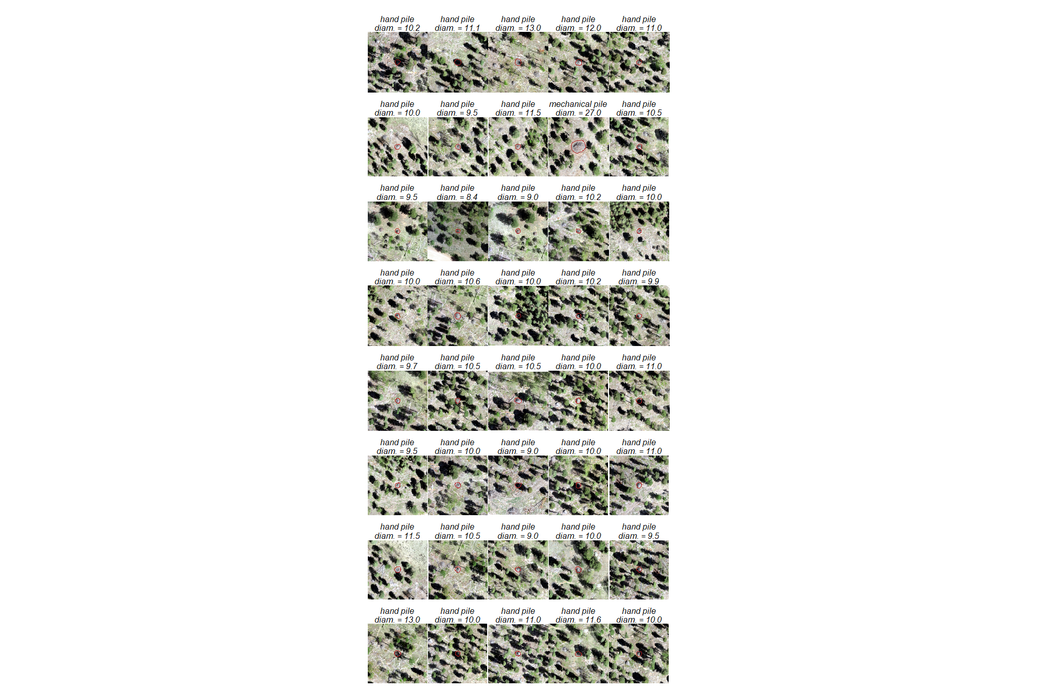
object-based image analysis will require polygon data so that we have sets of pixels (i.e. “objects”) to work with for training our model (nice, we’ll use the image-annotated pile data)
another challenge will be training a spectral-based model with the different lighting conditions in the imagery (e.g. piles in shadows or under tree crowns). this different lighting may have also influenced the point cloud generation
2.4 Point Cloud Data
Let’s check out the point cloud data we got using UAS-SfM methods
# directory with the downloaded .las|.laz files
f_temp <-
  "f:\\PFDP_Data\\p4pro_images\\P4Pro_06_17_2021_half_half_optimal\\2_densification\\point_cloud"
  # system.file(package = "lidR", "extdata", "Megaplot.laz")
# is there data?
list.files(f_temp, pattern = ".*\\.(laz|las)$") %>% length()
## [1] 1## [1] "P4Pro_06_17_2021_half_half_optimal_group1_densified_point_cloud.las"what information does lidR read from the catalog?
las_ctg <- lidR::readLAScatalog(f_temp)
# set the processing options
lidR::opt_progress(las_ctg) <- F
lidR::opt_filter(las_ctg) <- "-drop_duplicates"
lidR::opt_select(las_ctg) <- "xyziRGB"
# huh?
las_ctg
## class : LAScatalog (v1.2 format 3)
## extent : 499264.2, 499958.8, 4317541, 4318147 (xmin, xmax, ymin, ymax)
## coord. ref. : WGS 84 / UTM zone 13N
## area : 420912.1 m²
## points : 158.01 million points
## type : terrestrial
## density : 375.4 points/m²
## num. files : 1that’s a lot of points…can an ordinary laptop handle it? we’ll find out.
We’ll plot our point cloud data tiles real quick to orient ourselves
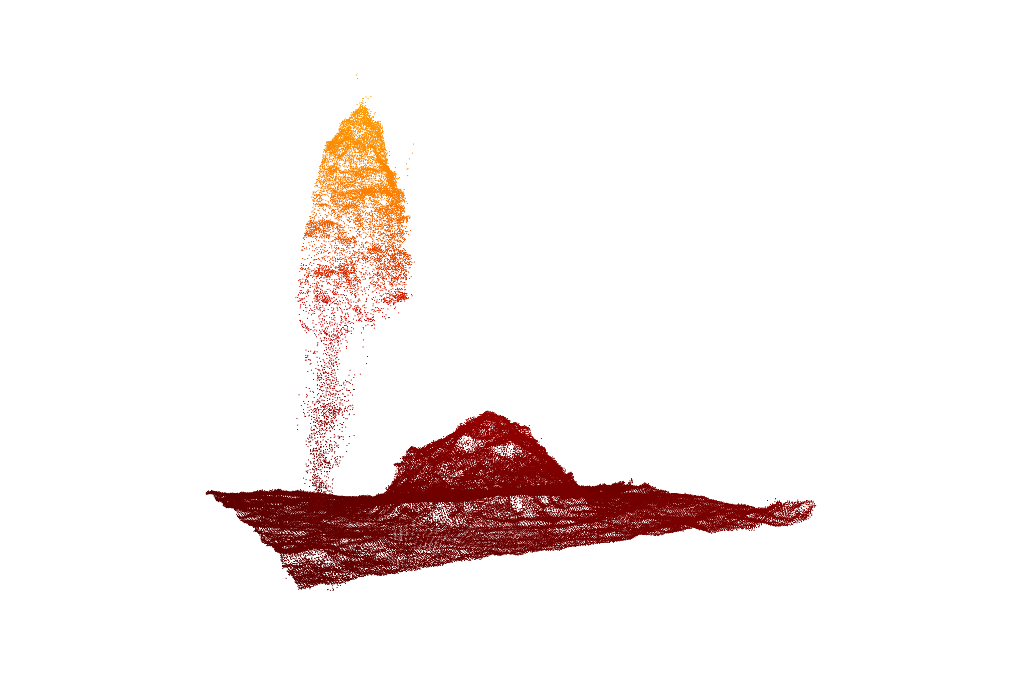
2.5 Check out one pile
las_temp <- lidR::clip_roi(
  las_ctg
  # biggest mechanical
  , slash_piles_points %>%
    dplyr::filter(tolower(comment)=="mechanical pile") %>%
    dplyr::arrange(desc(diameter)) %>%
    dplyr::slice(1) %>%
    sf::st_zm() %>%
    sf::st_buffer(10, endCapStyle = "SQUARE") %>%
    sf::st_transform(lidR::st_crs(las_ctg))
)
what did we get?
## Rows: 181,282
## Columns: 7
## $ X         <dbl> 499807.0, 499807.0, 499807.0, 499807.0, 499807.0, 499807.0, …
## $ Y         <dbl> 4317975, 4317975, 4317975, 4317975, 4317975, 4317975, 431797…
## $ Z         <dbl> 2714.829, 2714.777, 2714.709, 2714.900, 2714.636, 2714.594, …
## $ Intensity <int> 0, 0, 0, 0, 0, 0, 0, 0, 0, 0, 0, 0, 0, 0, 0, 0, 0, 0, 0, 0, …
## $ R         <int> 20224, 16896, 32256, 44288, 21760, 16896, 14592, 35584, 3148…
## $ G         <int> 18176, 16640, 34304, 40960, 20480, 14848, 8704, 34048, 34304…
## $ B         <int> 16384, 16384, 33280, 36608, 20992, 14336, 7168, 33280, 35072…
plot a sample
las_temp %>%
  lidR::plot(
    color = "Z", bg = "white", legend = F
   , pal = harrypotter::hp(n=50, house = "gryffindor")
  )
make a gif
library(magick)
if(!file.exists(file.path("../data/", "pile_z.gif"))){
  rgl::close3d()
  lidR::plot(
    las_temp, color = "Z", bg = "white", legend = F
   , pal = harrypotter::hp(n=50, house = "gryffindor")
  )
  rgl::movie3d( rgl::spin3d(), duration = 10, fps = 10 , movie = "pile_z", dir = "../data/")
  rgl::close3d()
}