Section 3 Point Cloud Processing

We’ll use the cloud2trees package to perform all preprocessing of point cloud data which includes:

• ground classification and noise removal
• raster data (DTM and CHM) generation
• point cloud height normalization

All of this can be accomplished using the cloud2trees::cloud2raster() function. After generating these products from the raw point cloud we’ll perform object segmentation to attempt to detect slash piles from the CHM which we’ll generate by setting the minimum height to zero (essentially a digital surface model [DSM] with the ground removed).

To attempt to identify slash piles from the CHM/DSM, we can use watershed segmentation or DBSCAN (Density-Based Spatial Clustering of Applications with Noise), for example. Both of these methods are common in segmenting individual trees and coarse woody debris from CHM data.

3.1 Process Raw Point Cloud

We’ll use cloud2trees::cloud2raster() to process the raw point cloud data. For each site we’ll generate a fine-resolution (0.1 m) CHM data set which can be aggregated to coarser resolution for sensitivity testing. Fine resolution CHM data would include granular details which may be important for delineating smaller slash piles while more coarse resolution data may help smooth out noise in the data to reduce false positive pile detections and potentially better represent the form of the actual piles

# set chm res
my_chm_res_m <- 0.1

3.1.1 PSINF Mixed Conifer Site

look at the summary of the point cloud data we’ll be processing

# processing dirs
c2t_out_dir_temp <- "../data/PFDP_Data/"
psinf_out_dir <- file.path(c2t_out_dir_temp, paste0("point_cloud_processing_delivery_chm",my_chm_res_m,"m") )
las_dir_temp <- "f:\\PFDP_Data\\p4pro_images\\P4Pro_06_17_2021_half_half_optimal\\2_densification\\point_cloud"

# read header with catalog
lidR::readLAScatalog(las_dir_temp)

## class       : LAScatalog (v1.2 format 3)
## extent      : 499264.2, 499958.8, 4317541, 4318147 (xmin, xmax, ymin, ymax)
## coord. ref. : WGS 84 / UTM zone 13N 
## area        : 420912.1 m²
## points      : 158.01 million points
## type        : terrestrial
## density     : 375.4 points/m²
## num. files  : 1

process the point cloud with the cloud2trees::cloud2raster() workflow

# do it
if(!dir.exists(psinf_out_dir)){
  # start time
  my_st_temp <- Sys.time()
  message("starting psinf cloud2raster() step at ...", my_st_temp)
  # cloud2trees
  psinf_cloud2raster_ans <- cloud2trees::cloud2raster(
    output_dir = c2t_out_dir_temp
    , input_las_dir = las_dir_temp
    , accuracy_level = 2
    , keep_intrmdt = T
    , dtm_res_m = 0.25
    , chm_res_m = my_chm_res_m
    , min_height = 0 # effectively generates a DSM based on non-ground points
  )
  # end
  my_end_temp <- Sys.time()
  # rename
  file.rename(from = file.path(c2t_out_dir_temp,"point_cloud_processing_delivery"), to = psinf_out_dir)
  # timer
  dplyr::tibble(
    timer_cloud2raster_mins = difftime(my_end_temp, my_st_temp, units = c("mins")) %>% as.numeric() 
  ) %>% 
    readr::write_csv(file = file.path(psinf_out_dir,"processed_tracking_data.csv"), append = F, progress = F)
}else{
  dtm_temp <- terra::rast( file.path(psinf_out_dir, "dtm_0.25m.tif") )
  chm_temp <- terra::rast( file.path(psinf_out_dir, paste0("chm_", my_chm_res_m,"m.tif")) )
  # combine
  psinf_cloud2raster_ans <- list(
    "dtm_rast" = dtm_temp
    , "chm_rast" = chm_temp
  )
}

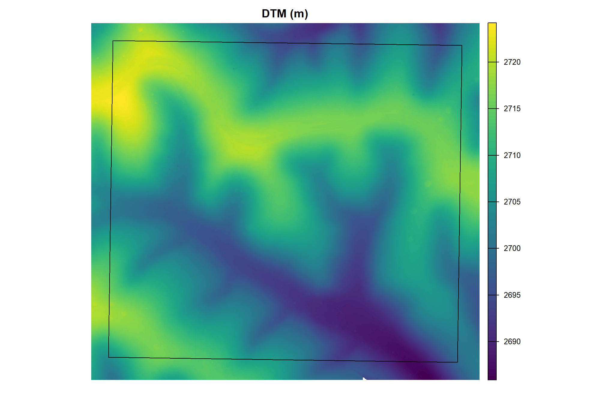
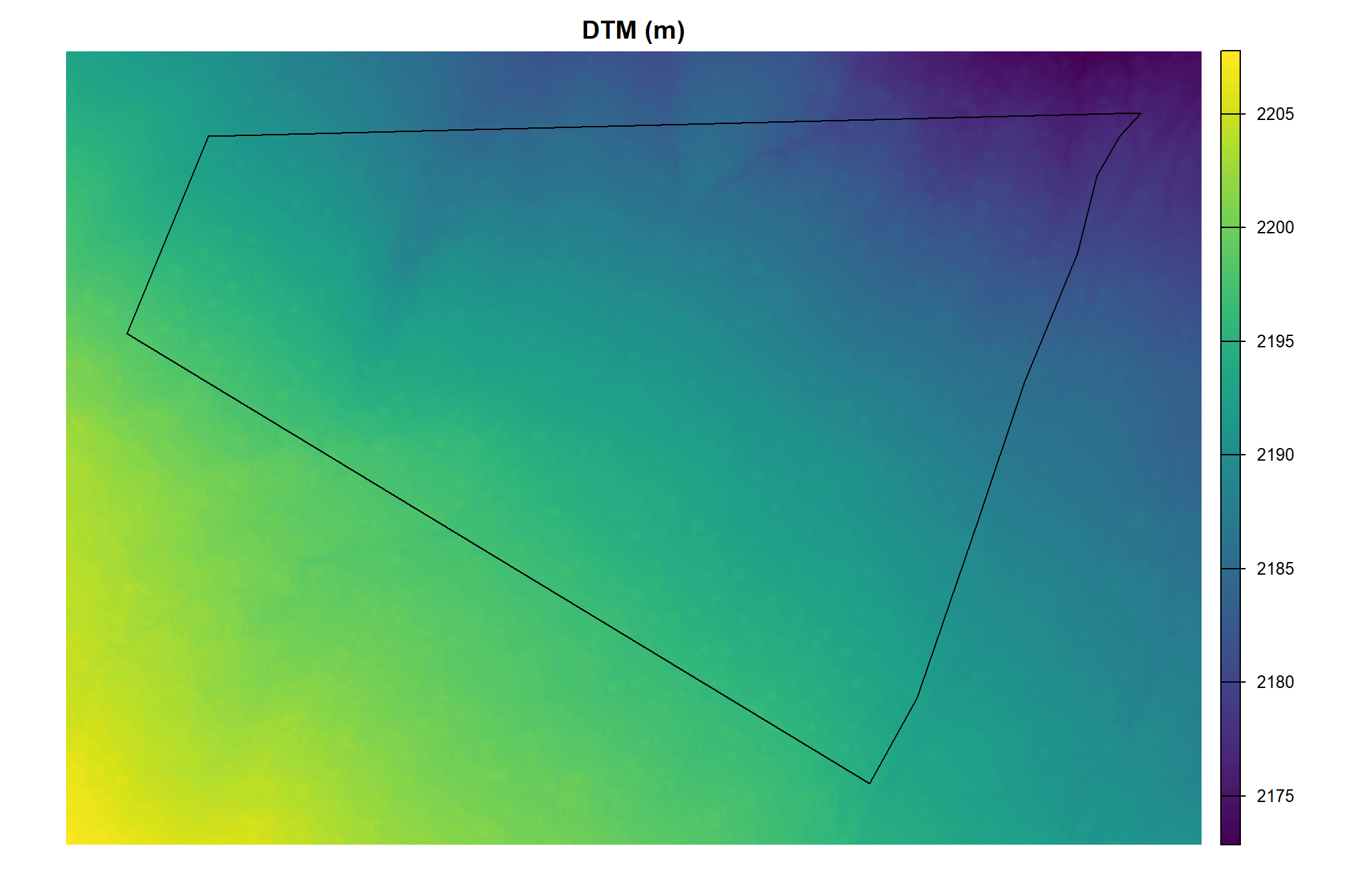
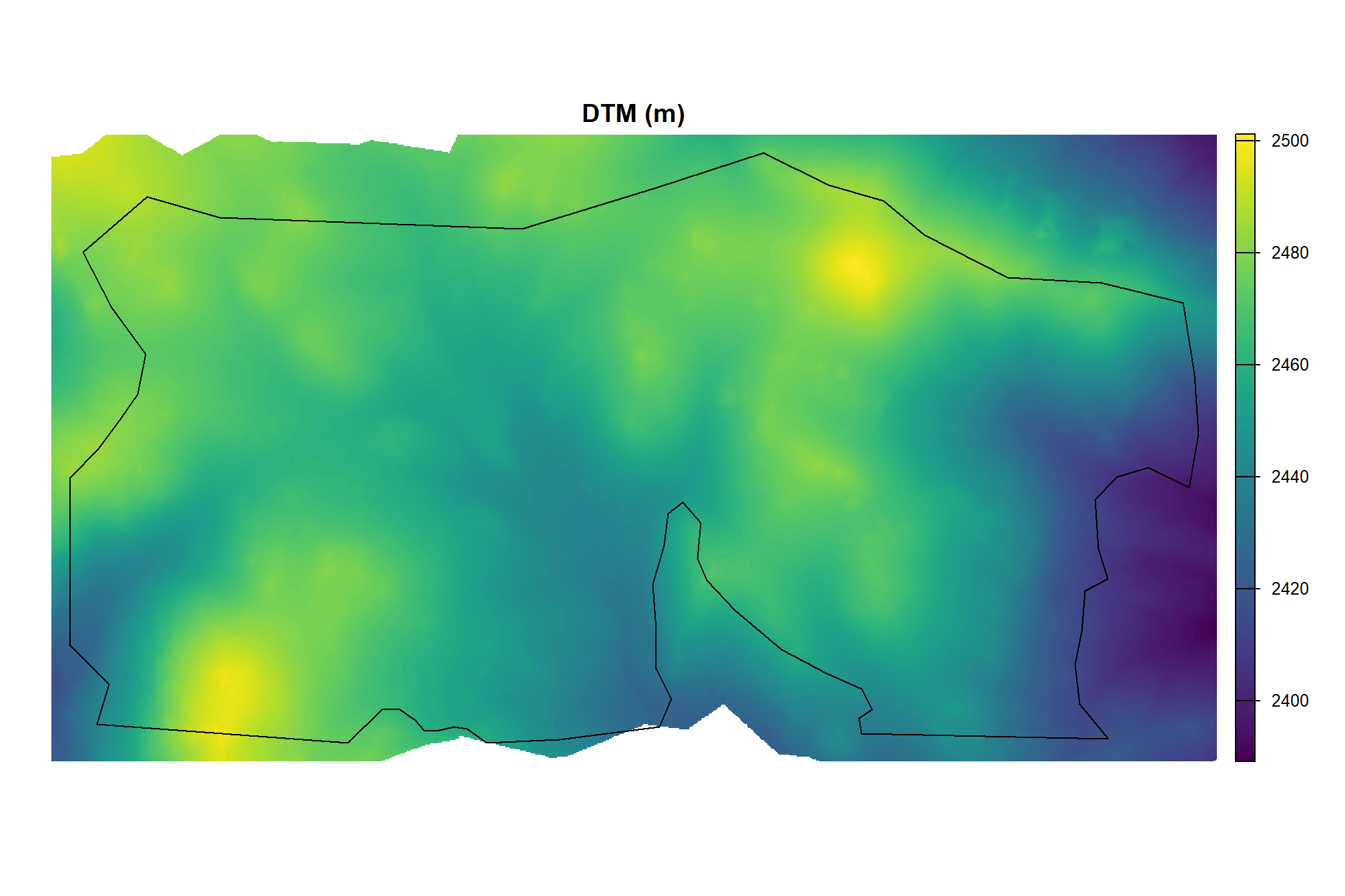
let’s check out the DTM

psinf_cloud2raster_ans$dtm_rast %>% 
  terra::crop(
    psinf_stand_boundary %>% 
    sf::st_buffer(22) %>% 
    sf::st_transform(terra::crs(psinf_cloud2raster_ans$dtm_rast)) %>% 
    terra::vect()
  ) %>% 
  terra::aggregate(fact = 2, na.rm = T, cores = lasR::half_cores()) %>%  
  terra::plot(
    col = viridis::viridis(n = 100)
    , axes = F
    , main = "DTM (m)"
  )
# add stand boundary
terra::plot(
  psinf_stand_boundary %>% 
    sf::st_transform(terra::crs(psinf_cloud2raster_ans$dtm_rast)) %>% 
    terra::vect()
  , add = T, border = "black", col = NA, lwd = 1.2
)

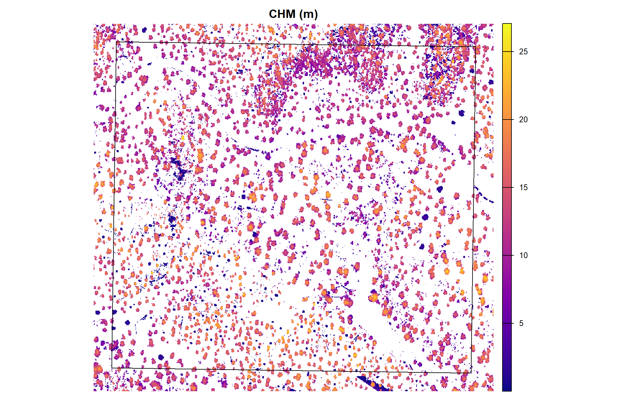
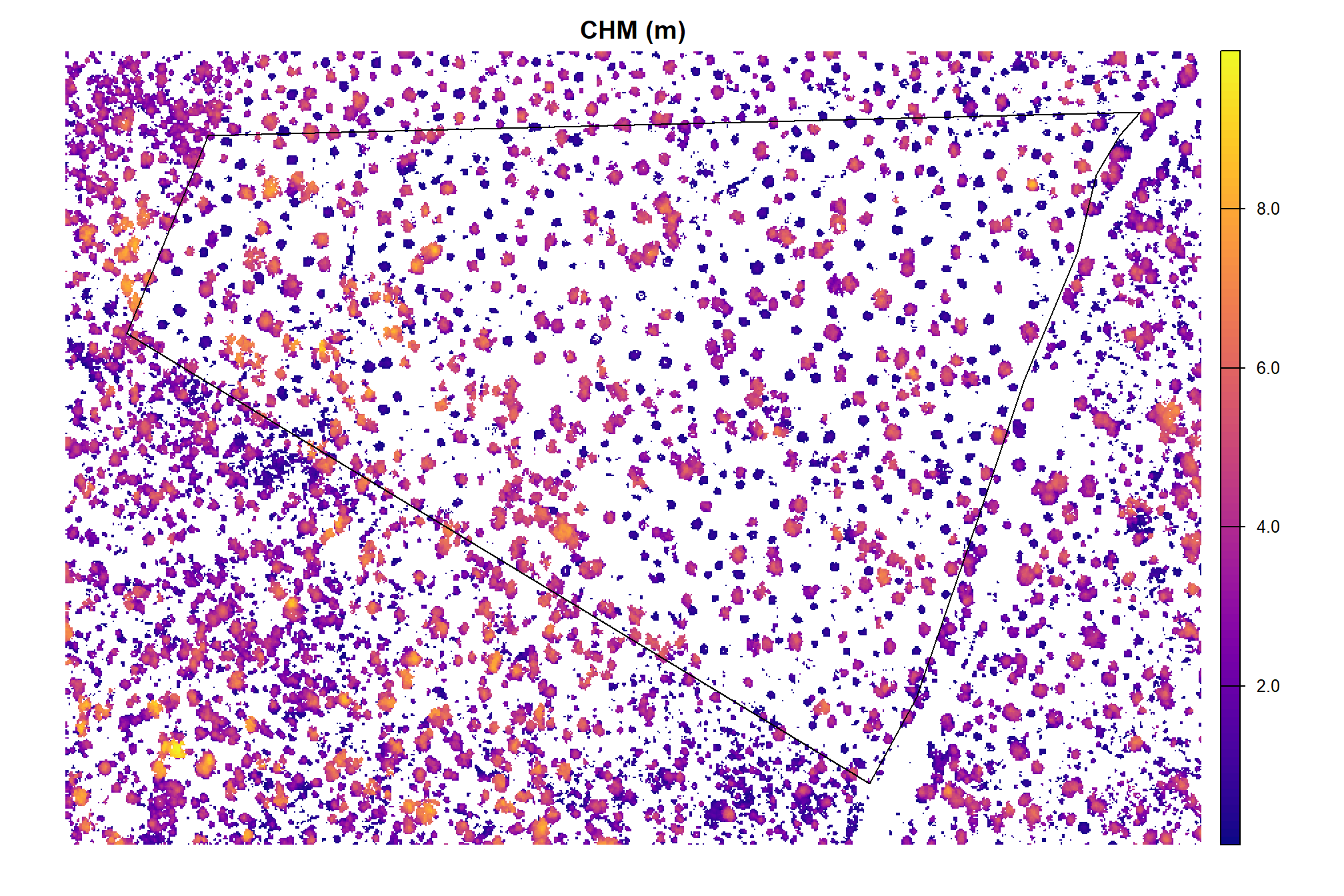
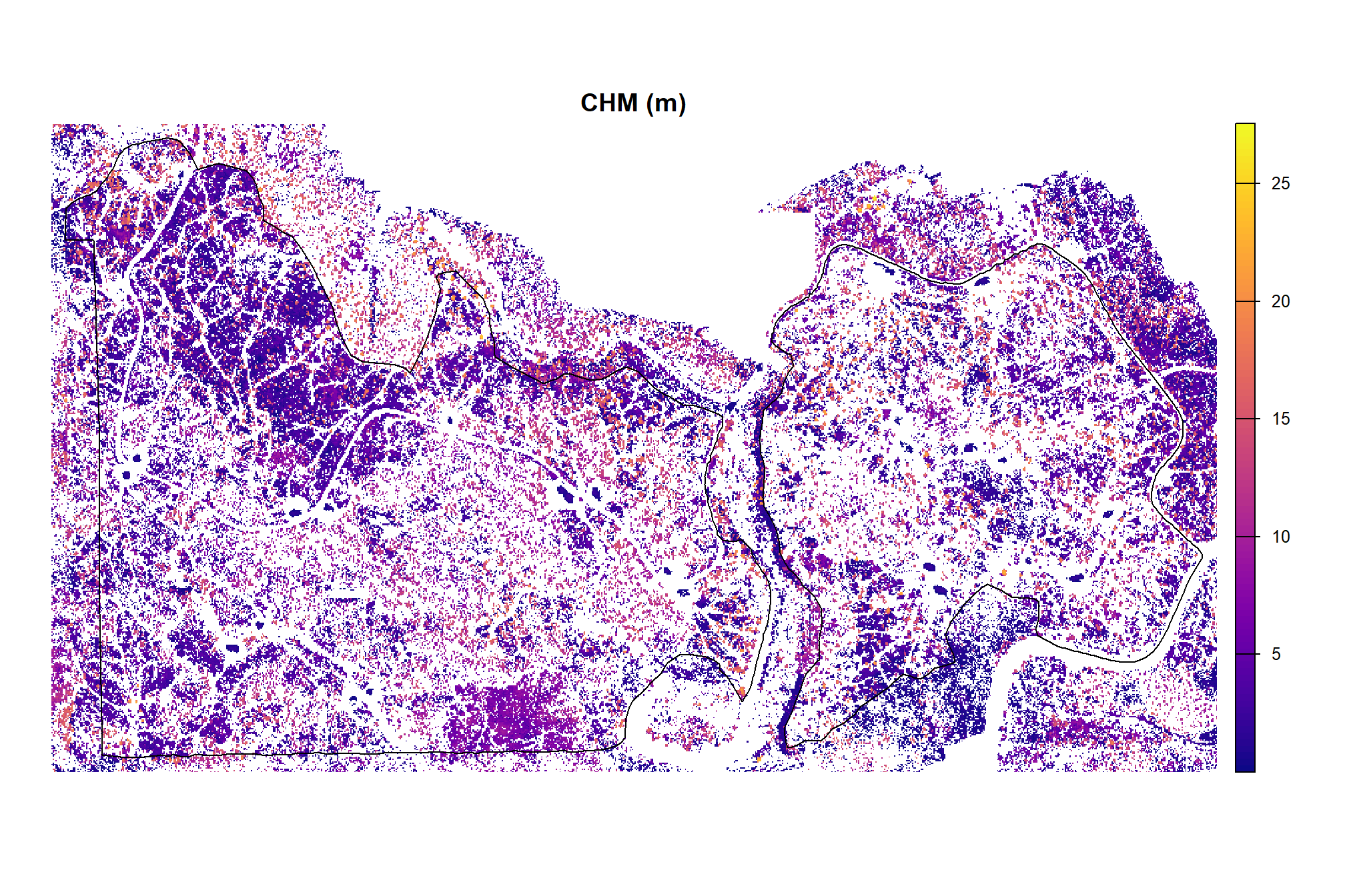
and CHM

psinf_cloud2raster_ans$chm_rast %>% 
  terra::crop(
    psinf_stand_boundary %>% 
    sf::st_buffer(22) %>% 
    sf::st_transform(terra::crs(psinf_cloud2raster_ans$chm_rast)) %>% 
    terra::vect()
  ) %>% 
  terra::aggregate(fact = 2, na.rm = T, cores = lasR::half_cores()) %>% 
  terra::plot(
    col = viridis::plasma(100)
    , axes = F
    , main = "CHM (m)"
  )
# add stand boundary
terra::plot(
  psinf_stand_boundary %>% 
    sf::st_transform(terra::crs(psinf_cloud2raster_ans$chm_rast)) %>% 
    terra::vect()
  , add = T, border = "black", col = NA, lwd = 1.2
)

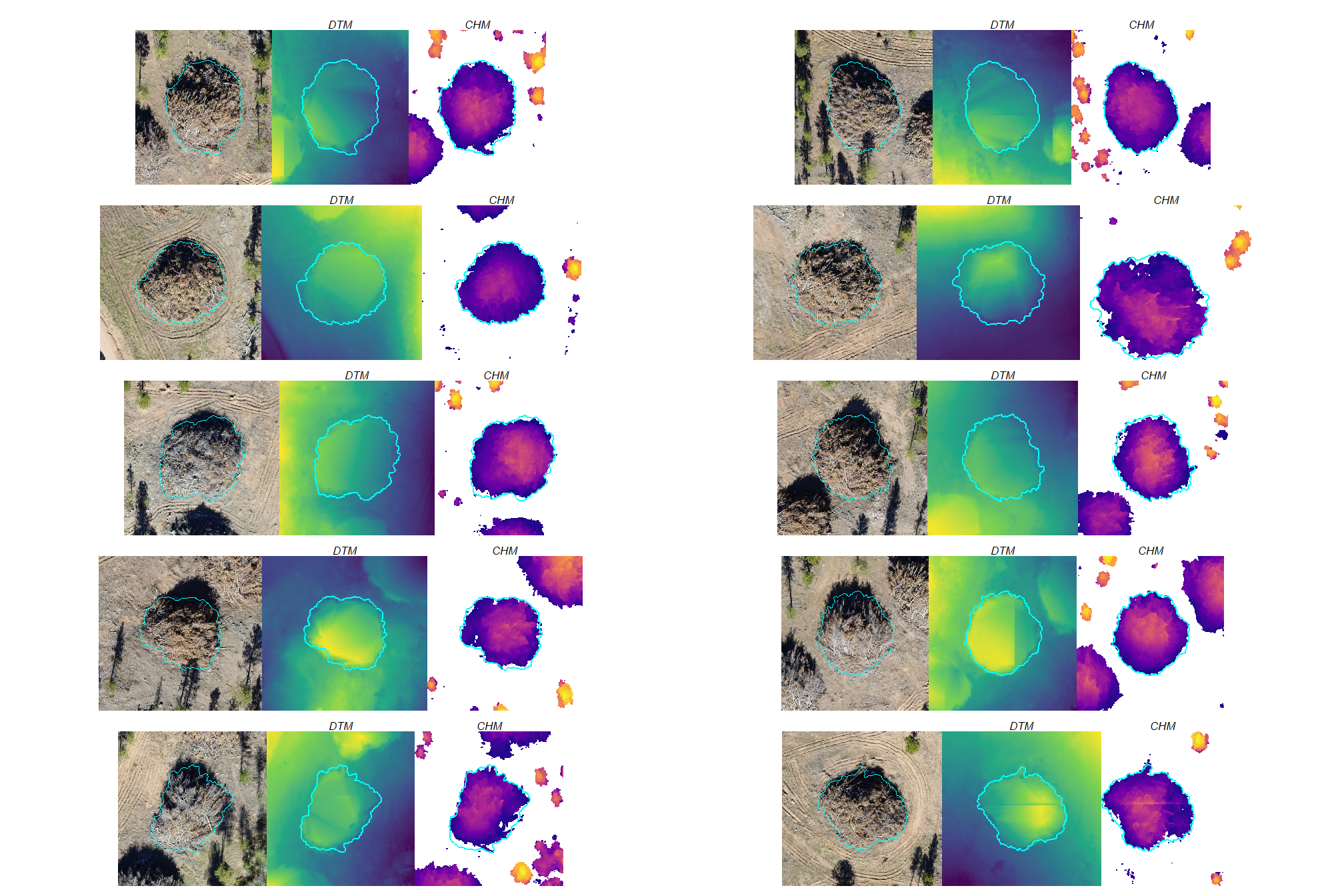
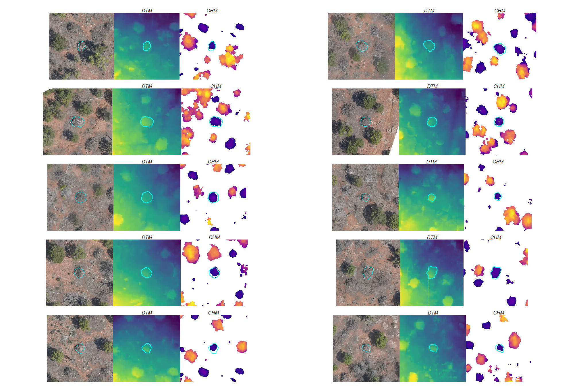
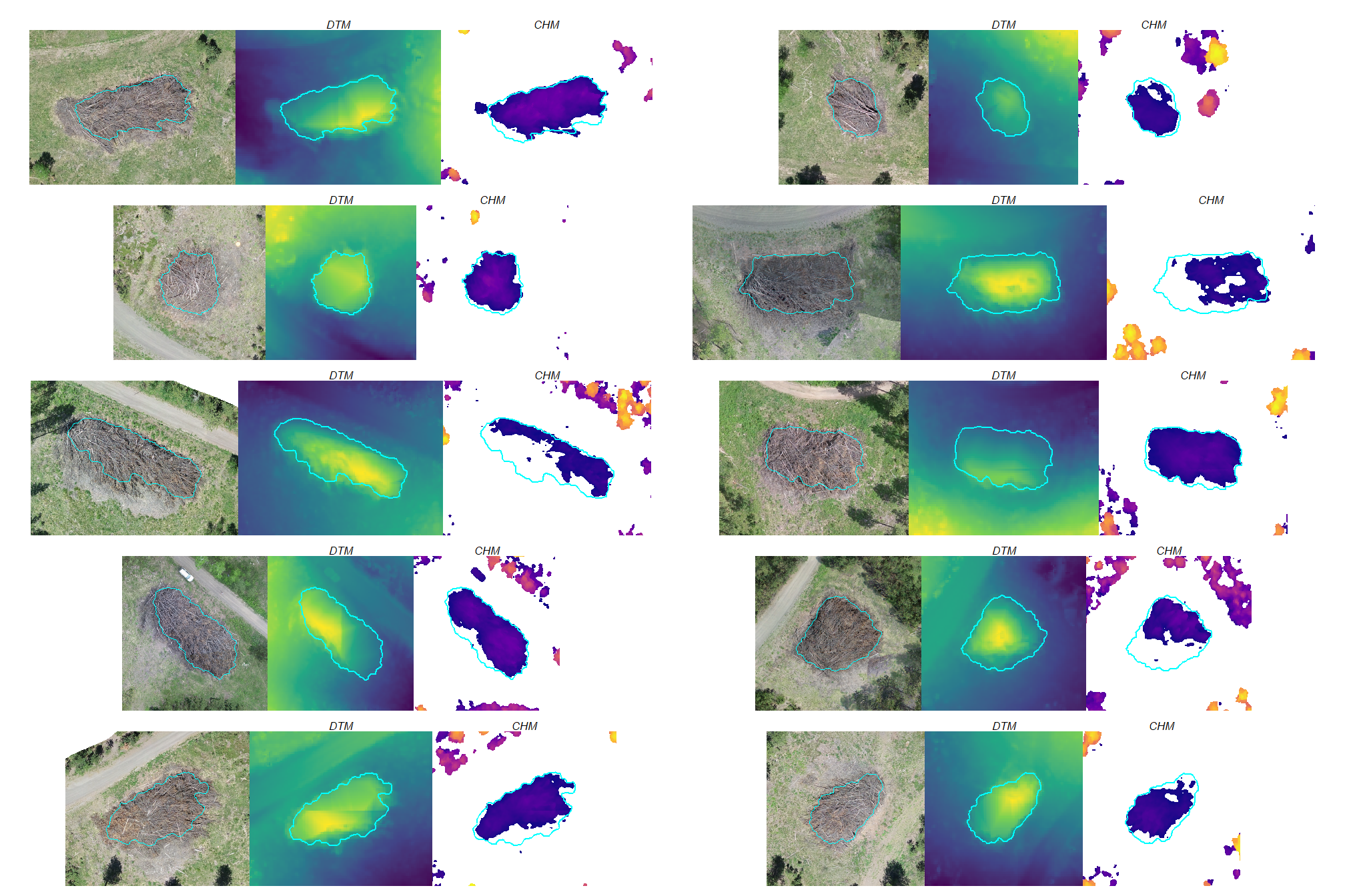
3.1.1.1 DTM and CHM + piles

let’s visually inspect the DTM and CHM with the pile outlines overlaid. we’ll make some functions to use for the different study areas

plt_rast_fn <- function(
    rn
    , df
    , rast
    , my_title = ""
    , vopt = "viridis"
    , lim = NULL
    , buff = 10
) {
  # scale the buffer based on the largest
    d_temp <- df %>%
      dplyr::arrange(desc(image_gt_diameter_m)) %>% 
      dplyr::slice(rn) %>% 
      sf::st_transform(terra::crs(rast))
    
    # convert rast to df
    comp_st <- rast %>%  
      terra::crop(
        d_temp %>% sf::st_buffer(buff) %>% terra::vect()
      ) %>% 
      terra::as.data.frame(xy = T) %>% 
      dplyr::rename(f=3)
    
    # ggplot
    comp_temp <- ggplot2::ggplot() +
      ggplot2::geom_tile(data = comp_st, ggplot2::aes(x=x,y=y,fill=f)) +
      ggplot2::geom_sf(data = d_temp, fill = NA, color = "cyan", lwd = 0.4) +
      ggplot2::scale_x_continuous(expand = c(0, 0)) +
      ggplot2::scale_y_continuous(expand = c(0, 0)) +
      ggplot2::labs(
        x = ""
        , y = ""
        , subtitle = my_title
      ) +
      ggplot2::theme_void() +
      ggplot2::theme(
        legend.position = "none" # c(0.5,1)
        , legend.margin = margin(0,0,0,0)
        , legend.text = element_text(size = 8)
        , legend.title = element_text(size = 8)
        , legend.key = element_rect(fill = "white")
        # , plot.title = ggtext::element_markdown(size = 10, hjust = 0.5)
        , plot.title = element_text(size = 8, hjust = 0.5, face = "bold")
        , plot.subtitle = element_text(size = 6, hjust = 0.5, face = "italic")
      )
  if(!is.null(lim)){
    comp_temp <- comp_temp + 
      ggplot2::scale_fill_viridis_c(option = vopt, limits = lim)
  }else{
    comp_temp <- comp_temp + 
      ggplot2::scale_fill_viridis_c(option = vopt)
  }
    
  plt_temp <- comp_temp
  return(list("plt"=plt_temp,"d"=d_temp))
}

# plt_rast_fn(rn = 9, df = psinf_slash_piles_polys, rast = psinf_cloud2raster_ans$dtm_rast, vopt = "viridis")

# combine 3
plt_rast_combine <- function(
    rn
    , df
    , dtm_rast
    , dtm_rast_vopt = "viridis"
    , chm_rast
    , chm_rast_vopt = "plasma"
    , rgb_rast
    , buffer = 10
) {
  # composite 1
  ans1 <- plt_rast_fn(
    rn = rn
    , df = df
    , rast = dtm_rast
    , my_title = "DTM"
    , vopt = dtm_rast_vopt
    , buff = buffer
  )
  # composite 2
  ans2 <- plt_rast_fn(
    rn = rn
    , df = df
    , rast = chm_rast
    , my_title = "CHM"
    , vopt = chm_rast_vopt
    , buff = buffer
  )
  # plt rgb
    rgb_temp <-
      ortho_plt_fn(
        rgb_rast = rgb_rast
        , stand =ans1$d
        , buffer = buffer
        , add_stand = F
      ) + 
      ggplot2::geom_sf(data = ans1$d, fill = NA, color = "cyan", lwd = 0.3)
  # combine
    r <- patchwork::wrap_plots(list(rgb_temp,ans1$plt,ans2$plt), nrow = 1)
    return(r)
}

# plt_rast_combine(
#   rn = 11
#   , df = psinf_slash_piles_polys %>% dplyr::filter(is_in_stand)
#   , dtm_rast = psinf_cloud2raster_ans$dtm_rast
#   , chm_rast = psinf_cloud2raster_ans$chm_rast
#   , rgb_rast = psinf_rgb_rast
# )

use this handy plotting function for some piles

# add pile locations
plt_list_rast_temp <- 
  1:sum(psinf_slash_piles_polys$is_in_stand) %>% 
  sample(
    min(10, sum(psinf_slash_piles_polys$is_in_stand))
  ) %>% 
  purrr::map(
    \(x) 
    plt_rast_combine(
      rn = x
      , df = psinf_slash_piles_polys %>% dplyr::filter(is_in_stand)
      , dtm_rast = psinf_cloud2raster_ans$dtm_rast
      , chm_rast = psinf_cloud2raster_ans$chm_rast
      , rgb_rast = psinf_rgb_rast
    )
  )
# plt_list_rast_temp[[2]]

combine the plots with patchwork

patchwork::wrap_plots(
  plt_list_rast_temp
  , ncol = 2
)

a few things are noteworthy in these examples:

• Piles are clearly visible in some areas of the DTM but less visible in other areas
• Piles are delineated in the CHM but with varying degrees of definition based on surrounding terrain and pile structure
• The DTM and CHM were rarely impacted by shadows in the RGB imagery
• It is interesting to see coarse woody debris occasionally visible in the CHM

3.1.2 TRFO-BLM Pinyon-Juniper Site

for this site, the full point cloud data we have covers a much larger extent than the treatment unit used for this study. we will therefore crop point cloud to a buffered area of interest so that we limit the amount of data processed

###############################################################
# read/crop point cloud
###############################################################
# output dir for clipped las
las_dir_temp <- "../data/Dawson_Data/point_cloud" 
if(!dir.exists(las_dir_temp)){dir.create(las_dir_temp, showWarnings = F)}
# do it if not already done
if(dplyr::coalesce(length(list.files(las_dir_temp)),0)<1){
  # this reads the metadata from all files in the folder, not the points themselves.
  las_ctg_temp <- lidR::readLAScatalog("d:/BLM_CO_SWDF_DawsonFuelsTreatment/Final/PointCloud/Tiles/")
  las_ctg_temp
  cloud2trees:::check_las_ctg_empty(las_ctg_temp)
  # set ctg opts
  lidR::opt_select(las_ctg_temp) <- "xyzainrcRGBNC"
  lidR::opt_progress(las_ctg_temp) <- T
  # write generated results to disk storage rather than keeping everything in memory. This option can be activated with opt_output_files()
  lidR::opt_output_files(las_ctg_temp) <- paste0(normalizePath(las_dir_temp),"/", "_{XLEFT}_{YBOTTOM}") # label outputs based on coordinates
  lidR::opt_filter(las_ctg_temp) <- "-drop_duplicates"
  
  # clip the point cloud using the polygon and write to a new file
  # the lidR::opt_output_files is key to writing the output to disk without loading the entire clipped result into memory.
  clip_las_ctg_temp <- lidR::clip_roi(
    las = las_ctg_temp
    , geometry = pj_stand_boundary %>% 
      sf::st_buffer(100) %>% 
      sf::st_bbox() %>% 
      sf::st_as_sfc() %>% 
      sf::st_as_sf() %>% 
      sf::st_transform(sf::st_crs(las_ctg_temp))
  )
}else{
  clip_las_ctg_temp <- lidR::readLAScatalog(las_dir_temp)
}
# clip_las_ctg_temp
# clip_las_ctg_temp$filename

look at the summary of the point cloud data we’ll be processing

# processing dirs
c2t_out_dir_temp <- "../data/Dawson_Data/"
pj_out_dir <- file.path(c2t_out_dir_temp, paste0("point_cloud_processing_delivery_chm",my_chm_res_m,"m") )
# las_dir_temp <- las_dir_temp
# read header with catalog
lidR::readLAScatalog(las_dir_temp)

## class       : LAScatalog (v1.2 format 2)
## extent      : 707813.6, 708409.9, 4193155, 4193638 (xmin, xmax, ymin, ymax)
## coord. ref. : NAD83(2011) / UTM zone 12N 
## area        : 288106.3 m²
## points      : 163.84 million points
## type        : terrestrial
## density     : 568.7 points/m²
## density     : 568.7 pulses/m²
## num. files  : 1

process the point cloud with the cloud2trees::cloud2raster() workflow

# do it
if(!dir.exists(pj_out_dir)){
  # start time
  my_st_temp <- Sys.time()
  message("starting pj cloud2raster() step at ...", my_st_temp)
  # cloud2trees
  pj_cloud2raster_ans <- cloud2trees::cloud2raster(
    output_dir = c2t_out_dir_temp
    , input_las_dir = las_dir_temp
    , accuracy_level = 2
    , keep_intrmdt = T
    , dtm_res_m = 0.2
    , chm_res_m = my_chm_res_m
    , min_height = 0 # effectively generates a DSM based on non-ground points
  )
  # end
  my_end_temp <- Sys.time()
  # rename
  file.rename(from = file.path(c2t_out_dir_temp,"point_cloud_processing_delivery"), to = pj_out_dir)
  # timer
  dplyr::tibble(
    timer_cloud2raster_mins = difftime(my_end_temp, my_st_temp, units = c("mins")) %>% as.numeric() 
  ) %>% 
    readr::write_csv(file = file.path(pj_out_dir,"processed_tracking_data.csv"), append = F, progress = F)
  
}else{
  dtm_temp <- terra::rast( file.path(pj_out_dir, "dtm_0.2m.tif") ) %>% 
    terra::aggregate(fact = 2, na.rm=T, cores = lasR::half_cores())
  chm_temp <- terra::rast( file.path(pj_out_dir, paste0("chm_", my_chm_res_m,"m.tif")) )
  # combine
  pj_cloud2raster_ans <- list(
    "dtm_rast" = dtm_temp
    , "chm_rast" = chm_temp
  )
}

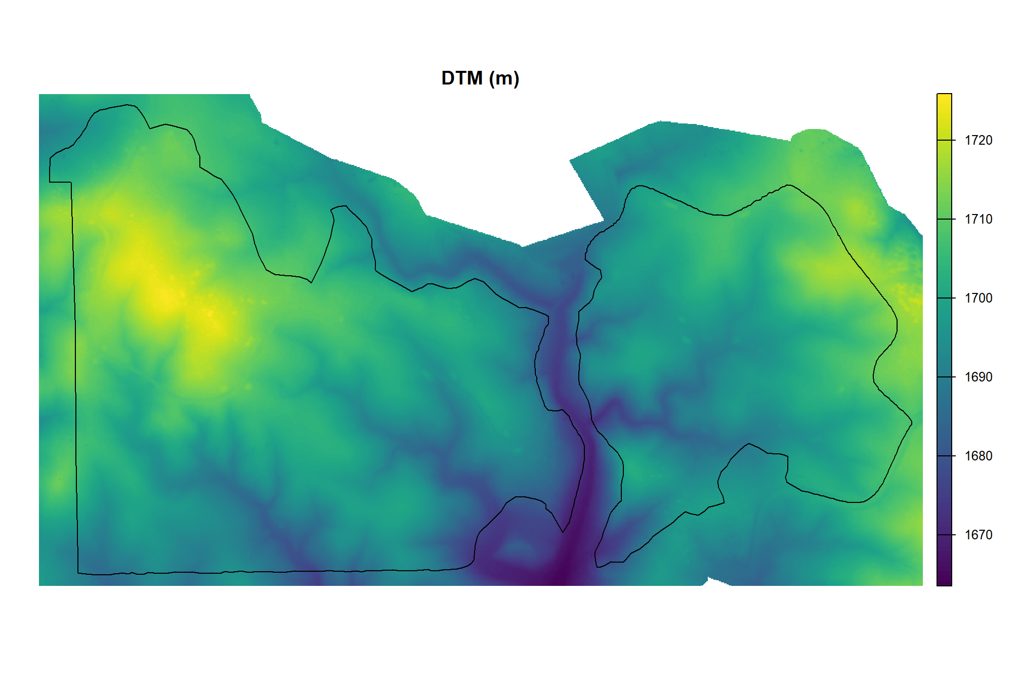
let’s check out the DTM

pj_cloud2raster_ans$dtm_rast %>% 
  terra::crop(
    pj_stand_boundary %>% 
    sf::st_buffer(22) %>% 
    sf::st_transform(terra::crs(pj_cloud2raster_ans$dtm_rast)) %>% 
    terra::vect()
  ) %>% 
  terra::plot(
    col = viridis::viridis(n = 100)
    , axes = F
    , main = "DTM (m)"
  )
# add stand boundary
terra::plot(
  pj_stand_boundary %>% 
    sf::st_transform(terra::crs(pj_cloud2raster_ans$dtm_rast)) %>% 
    terra::vect()
  , add = T, border = "black", col = NA, lwd = 1.2
)

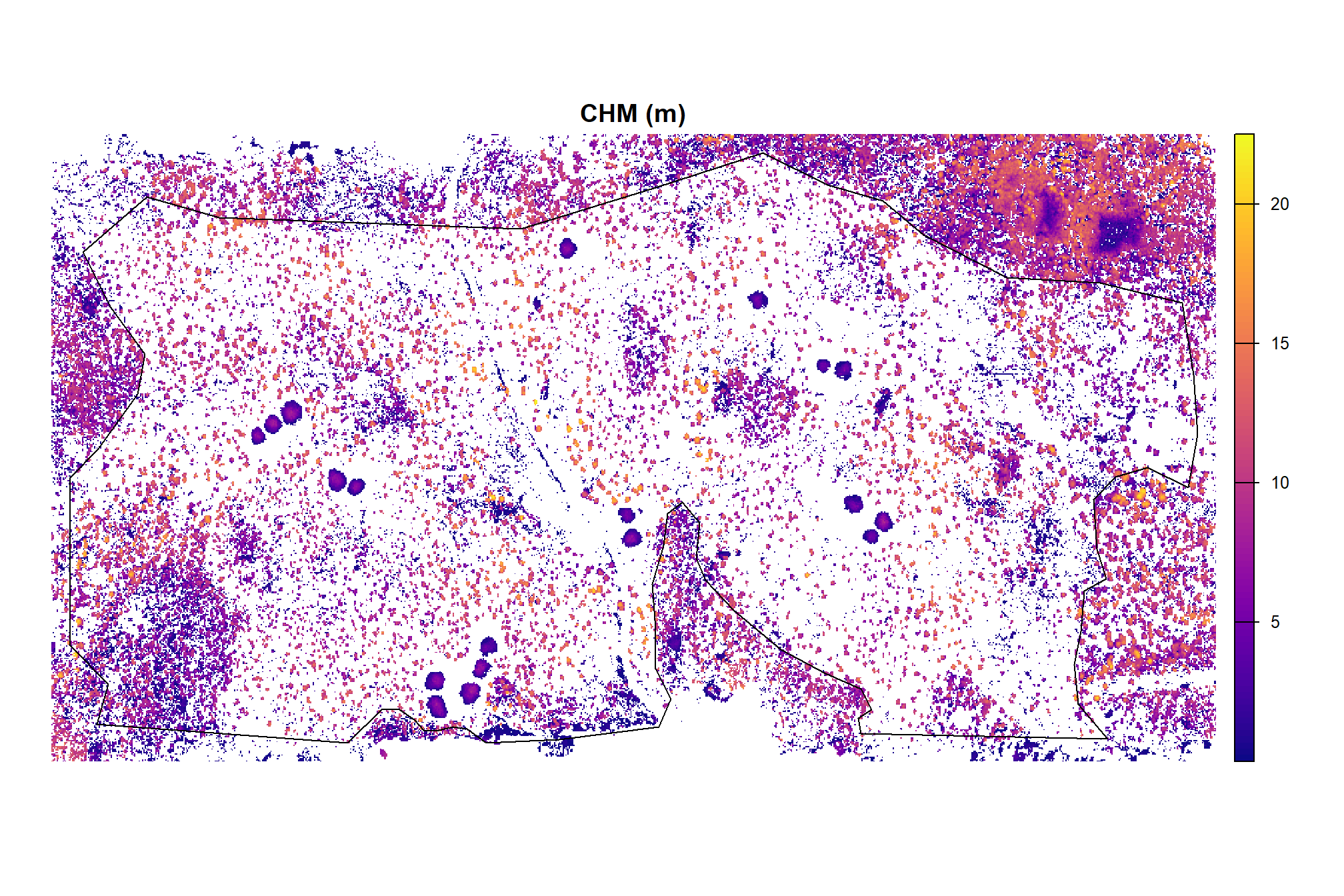
and CHM

pj_cloud2raster_ans$chm_rast %>% 
  terra::crop(
    pj_stand_boundary %>% 
    sf::st_buffer(22) %>% 
    sf::st_transform(terra::crs(pj_cloud2raster_ans$chm_rast)) %>% 
    terra::vect()
  ) %>% 
  terra::aggregate(fact = 2, na.rm = T, cores = lasR::half_cores()) %>% 
  terra::plot(
    col = viridis::plasma(100)
    , axes = F
    , main = "CHM (m)"
  )
# add stand boundary
terra::plot(
  pj_stand_boundary %>% 
    sf::st_transform(terra::crs(pj_cloud2raster_ans$chm_rast)) %>% 
    terra::vect()
  , add = T, border = "black", col = NA, lwd = 1.2
)

3.1.2.1 DTM and CHM + piles

let’s visually inspect the DTM and CHM with the pile outlines overlaid for a sample of piles

# add pile locations
plt_list_rast_temp <- 
  1:sum(pj_slash_piles_polys$is_in_stand) %>% 
  sample(
    min(10, sum(pj_slash_piles_polys$is_in_stand))
  ) %>% 
  purrr::map(
    \(x) 
    plt_rast_combine(
      rn = x
      , df = pj_slash_piles_polys %>% dplyr::filter(is_in_stand)
      , dtm_rast = pj_cloud2raster_ans$dtm_rast
      , chm_rast = pj_cloud2raster_ans$chm_rast
      , rgb_rast = pj_rgb_rast
    )
  )
# plt_list_rast_temp[[2]]

combine the plots with patchwork

patchwork::wrap_plots(
  plt_list_rast_temp
  , ncol = 2
)

3.1.3 BHEF Ponderosa Pine Site

for this site, the point cloud files are dispersed across different folders. so, we’ll manually specify which files to use.

look at the summary of the point cloud data we’ll be processing

# processing dirs
c2t_out_dir_temp <- "../data/BHEF_202306/"
bhef_out_dir <- file.path(c2t_out_dir_temp, paste0("point_cloud_processing_delivery_chm",my_chm_res_m,"m") )
# las_dir_temp <- "where/are/the/pointcloud"
las_flist_temp <- c(
  "F:\\UAS_Collections\\BHEF_202306/Unit1and3Processing.files/BHEF_202306_Unit1and3_laz.laz"
  , "F:\\UAS_Collections\\BHEF_202306/Unit2Processing.files/BHEF_202306_Unit2_laz.laz"        
  , list.files(
    "F:\\UAS_Collections\\BHEF_202306\\00good_simplified_point_clouds_reduced_overlap"
    , pattern = ".*\\.(laz|las)$"
    , full.names = TRUE, recursive = T
  )
)

# read header with catalog
lidR::readLAScatalog(las_flist_temp)

## class       : LAScatalog (v1.2 format 2)
## extent      : 608234, 610968.2, 4888216, 4889418 (xmin, xmax, ymin, ymax)
## coord. ref. : NAD83 / UTM zone 13N 
## area        : 3.48 km²
## points      : 1.42 billion points
## type        : airborne
## density     : 408 points/m²
## density     : 408 pulses/m²
## num. files  : 7

process the point cloud with the cloud2trees::cloud2raster() workflow

# do it
if(!dir.exists(bhef_out_dir)){
  # start time
  my_st_temp <- Sys.time()
  message("starting bhef cloud2raster() step at ...", my_st_temp)
  # cloud2trees
  bhef_cloud2raster_ans <- cloud2trees::cloud2raster(
    output_dir = c2t_out_dir_temp
    , input_las_dir = las_flist_temp
    , accuracy_level = 2
    , keep_intrmdt = T
    , dtm_res_m = 0.2
    , chm_res_m = my_chm_res_m
    , min_height = 0 # effectively generates a DSM based on non-ground points
  )
  # end
  my_end_temp <- Sys.time()
  # rename
  file.rename(from = file.path(c2t_out_dir_temp,"point_cloud_processing_delivery"), to = bhef_out_dir)
  # timer
  dplyr::tibble(
    timer_cloud2raster_mins = difftime(my_end_temp, my_st_temp, units = c("mins")) %>% as.numeric() 
  ) %>% 
    readr::write_csv(file = file.path(bhef_out_dir,"processed_tracking_data.csv"), append = F, progress = F)
  
}else{
  dtm_temp <- terra::rast( file.path(bhef_out_dir, "dtm_0.2m.tif") ) %>% 
    terra::aggregate(fact = 2, na.rm=T, cores = lasR::half_cores())
  chm_temp <- terra::rast( file.path(bhef_out_dir, paste0("chm_", my_chm_res_m,"m.tif")) )
  # combine
  bhef_cloud2raster_ans <- list(
    "dtm_rast" = dtm_temp
    , "chm_rast" = chm_temp
  )
}

let’s check out the DTM

bhef_cloud2raster_ans$dtm_rast %>% 
  terra::crop(
    bhef_stand_boundary %>% 
    sf::st_buffer(22) %>% 
    sf::st_transform(terra::crs(bhef_cloud2raster_ans$dtm_rast)) %>% 
    terra::vect()
  ) %>% 
  terra::plot(
    col = viridis::viridis(n = 100)
    , axes = F
    , main = "DTM (m)"
  )
# add stand boundary
terra::plot(
  bhef_stand_boundary %>% 
    sf::st_transform(terra::crs(bhef_cloud2raster_ans$dtm_rast)) %>% 
    terra::vect()
  , add = T, border = "black", col = NA, lwd = 1.2
)

and CHM

bhef_cloud2raster_ans$chm_rast %>% 
  terra::crop(
    bhef_stand_boundary %>% 
    sf::st_buffer(22) %>% 
    sf::st_transform(terra::crs(bhef_cloud2raster_ans$chm_rast)) %>% 
    terra::vect()
  ) %>% 
  terra::aggregate(fact = 2, na.rm = T, cores = lasR::half_cores()) %>%  
  terra::plot(
    col = viridis::plasma(100)
    , axes = F
    , main = "CHM (m)"
  )
# add stand boundary
terra::plot(
  bhef_stand_boundary %>% 
    sf::st_transform(terra::crs(bhef_cloud2raster_ans$chm_rast)) %>% 
    terra::vect()
  , add = T, border = "black", col = NA, lwd = 1.2
)

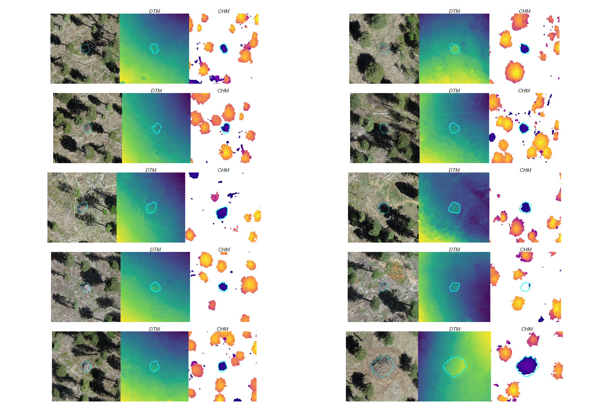
3.1.3.1 DTM and CHM + piles

let’s visually inspect the DTM and CHM with the pile outlines overlaid for a sample of piles

# add pile locations
plt_list_rast_temp <- 
  1:sum(bhef_slash_piles_polys$is_in_stand) %>% 
  sample(
    min(10, sum(bhef_slash_piles_polys$is_in_stand))
  ) %>% 
  purrr::map(
    \(x) 
    plt_rast_combine(
      rn = x
      , df = bhef_slash_piles_polys %>% dplyr::filter(is_in_stand)
      , dtm_rast = bhef_cloud2raster_ans$dtm_rast
      , chm_rast = bhef_cloud2raster_ans$chm_rast
      , rgb_rast = bhef_rgb_rast
    )
  )
# plt_list_rast_temp[[2]]

combine the plots with patchwork

patchwork::wrap_plots(
  plt_list_rast_temp
  , ncol = 2
)

3.1.4 ARNF Ponderosa Pine Site

look at the summary of the point cloud data we’ll be processing

# processing dirs
c2t_out_dir_temp <- "../data/ARNF_DiamondView_202510/" # where do you want to save processed data to?
arnf_out_dir <- file.path(c2t_out_dir_temp, paste0("point_cloud_processing_delivery_chm",my_chm_res_m,"m") )
las_dir_temp <- "F:/UAS_Collections/ARNF_DiamondView_202510/point_cloud_high_density" # where is the raw las

# read header with catalog
lidR::readLAScatalog(las_dir_temp)

## class       : LAScatalog (v1.2 format 3)
## extent      : 455073.8, 456582.3, 4535127, 4536067 (xmin, xmax, ymin, ymax)
## coord. ref. : WGS 84 / UTM zone 13N 
## area        : 1.24 km²
## points      : 1.37 billion points
## type        : airborne
## density     : 1102.8 points/m²
## density     : 39.9 pulses/m²
## num. files  : 44

process the point cloud with the cloud2trees::cloud2raster() workflow

# do it
if(!dir.exists(arnf_out_dir)){
  # start time
  my_st_temp <- Sys.time()
  message("starting arnf cloud2raster() step at ...", my_st_temp)
  # cloud2trees
  arnf_cloud2raster_ans <- cloud2trees::cloud2raster(
    output_dir = c2t_out_dir_temp
    , input_las_dir = las_dir_temp
    , accuracy_level = 2
    , keep_intrmdt = T
    , dtm_res_m = 0.2
    , chm_res_m = my_chm_res_m
    , min_height = 0 # effectively generates a DSM based on non-ground points
  )
  # end
  my_end_temp <- Sys.time()
  # rename
  file.rename(from = file.path(c2t_out_dir_temp,"point_cloud_processing_delivery"), to = arnf_out_dir)
  # timer
  dplyr::tibble(
    timer_cloud2raster_mins = difftime(my_end_temp, my_st_temp, units = c("mins")) %>% as.numeric() 
  ) %>% 
    readr::write_csv(file = file.path(arnf_out_dir,"processed_tracking_data.csv"), append = F, progress = F)
}else{
  dtm_temp <- terra::rast( file.path(arnf_out_dir, "dtm_0.2m.tif") ) %>% 
    terra::aggregate(fact = 2, na.rm=T, cores = lasR::half_cores())
  chm_temp <- terra::rast( file.path(arnf_out_dir, paste0("chm_", my_chm_res_m,"m.tif")) )
  # combine
  arnf_cloud2raster_ans <- list(
    "dtm_rast" = dtm_temp
    , "chm_rast" = chm_temp
  )
}

let’s check out the DTM

arnf_cloud2raster_ans$dtm_rast %>% 
  terra::crop(
    arnf_stand_boundary %>% 
    sf::st_buffer(22) %>% 
    sf::st_transform(terra::crs(arnf_cloud2raster_ans$dtm_rast)) %>% 
    terra::vect()
  ) %>% 
  terra::plot(
    col = viridis::viridis(n = 100)
    , axes = F
    , main = "DTM (m)"
  )
# add stand boundary
terra::plot(
  arnf_stand_boundary %>% 
    sf::st_transform(terra::crs(arnf_cloud2raster_ans$dtm_rast)) %>% 
    terra::vect()
  , add = T, border = "black", col = NA, lwd = 1.2
)

and CHM

arnf_cloud2raster_ans$chm_rast %>% 
  terra::crop(
    arnf_stand_boundary %>% 
    sf::st_buffer(22) %>% 
    sf::st_transform(terra::crs(arnf_cloud2raster_ans$chm_rast)) %>% 
    terra::vect()
  ) %>% 
  terra::aggregate(fact = 2, na.rm = T, cores = lasR::half_cores()) %>% 
  terra::plot(
    col = viridis::plasma(100)
    , axes = F
    , main = "CHM (m)"
  )
# add stand boundary
terra::plot(
  arnf_stand_boundary %>% 
    sf::st_transform(terra::crs(arnf_cloud2raster_ans$chm_rast)) %>% 
    terra::vect()
  , add = T, border = "black", col = NA, lwd = 1.2
)

3.1.4.1 DTM and CHM + piles

let’s visually inspect the DTM and CHM with the pile outlines overlaid for a sample of piles

# add pile locations
plt_list_rast_temp <- 
  1:sum(arnf_slash_piles_polys$is_in_stand) %>% 
  sample(
    min(10, sum(arnf_slash_piles_polys$is_in_stand))
  ) %>% 
  purrr::map(
    \(x) 
    plt_rast_combine(
      rn = x
      , df = arnf_slash_piles_polys %>% dplyr::filter(is_in_stand)
      , dtm_rast = arnf_cloud2raster_ans$dtm_rast
      , chm_rast = arnf_cloud2raster_ans$chm_rast
      , rgb_rast = arnf_rgb_rast
    )
  )
# plt_list_rast_temp[[2]]

combine the plots with patchwork

patchwork::wrap_plots(
  plt_list_rast_temp
  , ncol = 2
)

3.2 Clean Up

going forward, we only need the CHM data, so we can drop the DTM data from our session