Section 8 Detection Accuracy

To this point we have:

In this section, we’ll evaluate the effectiveness of the proposed geometric, rules-based slash pile detection methodology by assessing its detection accuracy performance. We fully reviewed the detection accuracy assessment workflow here, but here is a quick overview:

Detection accuracy metrics are calculated by aggregating raw TP (true positive), FP (false positive; commission), and FN (false negative; omission) counts to quantify the method’s ability to find the piles. Aggregation of the instance matching allows us to evaluate omission rate (false negative rate or miss rate), commission rate (false positive rate), precision, recall (detection rate), and the F-score metric. As a reminder, true positive (TP) instances correctly match ground truth instances with a prediction, commission predictions do not match a ground truth instance (false positive; FP), and omissions are ground truth instances for which no predictions match (FN)

8.1 Instance Matching

The first step in evaluating the performance of our slash pile detection methodology is to perform instance matching. Instance matching is the process of checking our predictions of slash pile presence (or absence) against the actual pile locations in real life (we use image-annotated pile outlines as ground truth) to determine if the method correctly identifies presence and absence. We use the framework established by Puliti et al. (2023, p. 14) to validate detections based on an Intersection over Union (IoU) threshold. We set this threshold at 45% which is slightly more permissive than the 50% used by Puliti et al. (2023) for tree crowns to accommodate the fact that our target objects are located on the forest floor rather than in the canopy and are therefore subject to higher levels of occlusion from aerial data.

we reviewed this process and defined the function ground_truth_prediction_match() here

# map over ground_truth_prediction_match for dbscan
  dbscan_gt_pred_match <- 
    all_stand_boundary$site_data_lab %>% 
    purrr::set_names() %>% 
    purrr::map(
      \(x)
      ground_truth_prediction_match(
          ground_truth = slash_piles_polys[[x]] %>% 
            dplyr::filter(is_in_stand) %>% 
            sf::st_transform( sf::st_crs(dbscan_spectral_preds[[x]]) ) %>% 
            dplyr::arrange(desc(image_gt_area_m2)) # this is so the algorithm starts with the largest
          , gt_id = "pile_id"
          , predictions = dbscan_spectral_preds[[x]]
          , pred_id = "pred_id"
          , min_iou_pct = 0.45
        )
      , .progress = T
    )
# map over ground_truth_prediction_match for watershed
  watershed_gt_pred_match <- 
    all_stand_boundary$site_data_lab %>% 
    purrr::set_names() %>% 
    purrr::map(
      \(x)
      ground_truth_prediction_match(
          ground_truth = slash_piles_polys[[x]] %>% 
            dplyr::filter(is_in_stand) %>% 
            sf::st_transform( sf::st_crs(watershed_spectral_preds[[x]]) ) %>% 
            dplyr::arrange(desc(image_gt_area_m2)) # this is so the algorithm starts with the largest
          , gt_id = "pile_id"
          , predictions = watershed_spectral_preds[[x]]
          , pred_id = "pred_id"
          , min_iou_pct = 0.45
        )
      , .progress = T
    )
# watershed_gt_pred_match[["pj"]] %>% dplyr::count(pred_id) %>% dplyr::filter(n>1) %>% dplyr::arrange(desc(n))
# dbscan_gt_pred_match[["pj"]] %>% dplyr::count(pred_id) %>% dplyr::filter(n>1) %>% dplyr::arrange(desc(n))

let’s see what the instance matching data looks like

# what did we get?
dbscan_gt_pred_match[[1]] %>% 
  dplyr::glimpse()

## Rows: 24
## Columns: 6
## $ pile_id   <int> 7, 8, 4, 6, 15, 13, 17, 11, 10, 9, 19, 18, 2, 5, 12, 1, 14, …
## $ i_area    <dbl> 536.5570, 539.9044, 492.3933, 449.3572, 422.1786, 425.3035, …
## $ u_area    <dbl> 593.2048, 579.0174, 519.5787, 483.3788, 459.7354, 454.9364, …
## $ iou       <dbl> 0.9045055, 0.9324494, 0.9476780, 0.9296171, 0.9183078, 0.934…
## $ pred_id   <dbl> 24249, 23782, 12862, 23411, 15434, 14529, 7687, 16382, 22005…
## $ match_grp <ord> true positive, true positive, true positive, true positive, …

let’s quickly look at the distribution of IoU for the TP matches

# palette
pal_match_grp = c(
  "omission"=viridis::cividis(3)[1]
  , "commission"= viridis::cividis(3)[2]
  , "true positive"=viridis::cividis(3)[3]
)
# plot
iou_dta_temp <- 
  dplyr::bind_rows(
   dbscan_gt_pred_match %>% 
      purrr::imap(
        \(x,nm)
        x %>% 
        dplyr::filter(match_grp=="true positive") %>% 
        dplyr::mutate(
          site = all_stand_boundary %>% dplyr::filter(site_data_lab==nm) %>% dplyr::pull(site)
          , method = "dbscan"
        )
      ) %>% 
     dplyr::bind_rows()
   , watershed_gt_pred_match %>% 
      purrr::imap(
        \(x,nm)
        x %>% 
        dplyr::filter(match_grp=="true positive") %>% 
        dplyr::mutate(
          site = all_stand_boundary %>% dplyr::filter(site_data_lab==nm) %>% dplyr::pull(site)
          , method = "watershed"
        )
      ) %>% 
     dplyr::bind_rows()
  )
# plot it

iou_dta_temp %>% 
  dplyr::mutate(
    site = stringr::word(site)
    , method = method %>%
      factor(ordered = T) %>% 
      forcats::fct_recode("DBSCAN" = "dbscan", "Watershed" = "watershed")
  ) %>% 
  # dplyr::glimpse()
  ggplot2::ggplot(mapping = ggplot2::aes(x = iou)) +
  ggplot2::geom_vline(xintercept = 0.45, color = "gray", linetype = "dashed", lwd = 1.5) +
  ggplot2::geom_violin(
    mapping = ggplot2::aes(y = 0, color = match_grp, fill = match_grp)
    , alpha = 0.8
  ) +
  ggplot2::geom_boxplot(width = 0.1, fill = NA, outliers = F) +
  ggplot2::scale_color_manual(values=pal_match_grp) +
  ggplot2::scale_fill_manual(values=pal_match_grp) +
  ggplot2::scale_y_continuous(NULL,breaks=NULL) +
  ggplot2::scale_x_continuous(limits = c(0,1), labels=scales::percent, breaks = scales::breaks_extended(n=6)) +
  ggplot2::facet_grid(
    rows = dplyr::vars(site)
    , cols = dplyr::vars(method)
    # , scales = "free_y"
    , switch = "y"
    , axes = "all_x"
  ) +
  ggplot2::labs(
    color="",fill="",x="IoU of correct precitions"
  ) +
  ggplot2::theme_light() +
  ggplot2::theme(
    legend.position = "none"
    , strip.text = ggplot2::element_text(size = 10, color = "black", face = "bold")
    , axis.text.x = ggplot2::element_text(size = 9)
    , axis.text.y = ggplot2::element_blank()
    , axis.ticks.y = ggplot2::element_blank()
  )

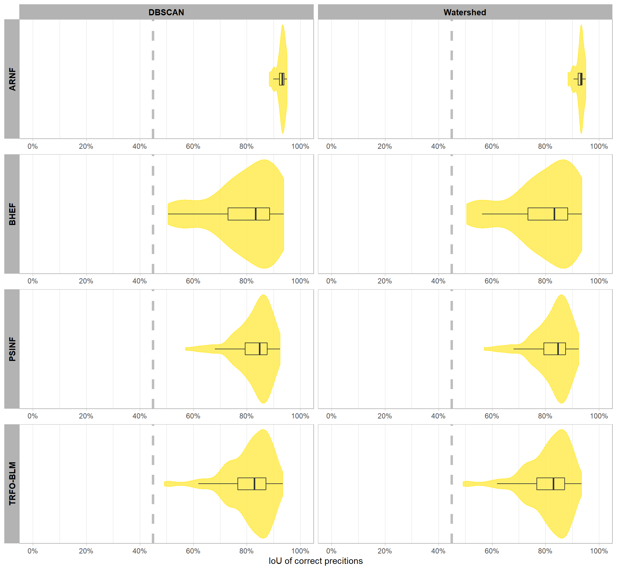
the majority of correct predictions had high overlap with the actual, ground truth piles with only a few piles at one site approaching the 45% minimum threshold to determine a match. let’s check out the summary stats

iou_dta_temp %>% 
  dplyr::group_by(site,method) %>% 
  dplyr::summarise(
    dplyr::across(
      c(iou)
      , .fns = list(
        mean = ~mean(.x,na.rm=T)
        , q50 = ~quantile(.x,na.rm=T,probs=0.5)
        , sd = ~sd(.x,na.rm=T)
        # , q10 = ~quantile(.x,na.rm=T,probs=0.1)
        # , q90 = ~quantile(.x,na.rm=T,probs=0.9)
        # , min = ~min(.x,na.rm=T)
        # , max = ~max(.x,na.rm=T)
        , range = ~paste0(
          scales::percent(min(.x,na.rm=T), accuracy = 0.1)
          ,"-"
          , scales::percent(max(.x,na.rm=T), accuracy = 0.1)
        )
      )
    )
    , n = dplyr::n() %>% scales::comma(accuracy = 1)
  ) %>% 
  dplyr::ungroup() %>% 
  dplyr::mutate(
    dplyr::across(
      dplyr::where(is.numeric)
      , ~scales::percent(.x,accuracy=0.1)
    )
  ) %>% 
  dplyr::relocate(site,method,n) %>% 
  dplyr::arrange(site,method) %>% 
  kableExtra::kbl(
    caption = "IoU of correct predictions (TP)"
    , col.names = c(
      "site", "method"
      , "TP predictions"
      , "IoU mean"
      , "IoU median"
      , "IoU sd"
      , "IoU range"
    )
    , escape = F
    # , digits = 2
  ) %>% 
  kableExtra::kable_styling() %>% 
  kableExtra::collapse_rows(columns = 1, valign = "top")

Table 8.1: IoU of correct predictions (TP)
site	method	TP predictions	IoU mean	IoU median	IoU sd	IoU range
ARNF Ponderosa Pine Site	dbscan	18	92.8%	93.2%	1.8%	88.4%-95.1%
ARNF Ponderosa Pine Site	watershed	18	92.8%	93.2%	1.8%	88.4%-95.1%
BHEF Ponderosa Pine Site	dbscan	24	79.1%	83.3%	12.3%	50.5%-93.7%
BHEF Ponderosa Pine Site	watershed	24	79.1%	83.3%	12.2%	50.5%-93.5%
PSINF Mixed Conifer Site	dbscan	115	82.8%	84.7%	6.8%	57.1%-92.5%
PSINF Mixed Conifer Site	watershed	115	82.8%	84.6%	6.8%	57.1%-92.5%
TRFO-BLM Pinyon-Juniper Site	dbscan	245	81.1%	82.9%	8.4%	49.2%-93.4%
TRFO-BLM Pinyon-Juniper Site	watershed	245	81.1%	82.9%	8.4%	49.2%-93.4%

let’s look at the results spatially noting that just because a prediction overlaps with a ground truth pile does not mean that it meets the IoU threshold for determining a positive match. in these cases where the IoU was insufficient, a commission (FP) will overlap with an omission (FN).

plt_fn_temp <- function(x, method) {
  if(tolower(method) == "dbscan"){
    preds <- dbscan_spectral_preds
    gt_pred_match <- dbscan_gt_pred_match
  }else if(tolower(method) == "watershed"){
    preds <- watershed_spectral_preds
    gt_pred_match <- watershed_gt_pred_match
  }else{return(NULL)}
  # plot it
    ggplot2::ggplot() +
      ggplot2::geom_sf(
        data = stand_boundary[[x]] %>% 
          sf::st_transform(sf::st_crs(preds[[x]]))
        , color = "black", fill = NA
      ) + 
      ggplot2::geom_sf(
        data = 
          slash_piles_polys[[x]] %>% 
            dplyr::filter(is_in_stand) %>% 
            dplyr::left_join(
              gt_pred_match[[x]] %>% 
                dplyr::select(pile_id,match_grp)
              , by = "pile_id"
            ) %>% 
            sf::st_transform(sf::st_crs(preds[[x]]))
        , mapping = ggplot2::aes(fill = match_grp)
        , color = NA ,alpha=0.7
        , show.legend = T
      ) + 
      ggplot2::geom_sf(
        data =
          preds[[x]] %>%
            dplyr::filter(is_in_stand) %>% 
            dplyr::left_join(
              gt_pred_match[[x]] %>% 
                dplyr::select(pred_id,match_grp)
              , by = "pred_id"
            )
        , mapping = ggplot2::aes(fill = match_grp, color = match_grp)
        , alpha = 0
        , lwd = 0.5
        , show.legend = T
      ) +
      ggplot2::scale_fill_manual(values = pal_match_grp, drop = F, name = "") +
      ggplot2::scale_color_manual(values = pal_match_grp, drop = F, name = "") +
      ggplot2::labs(
        subtitle = paste0(
          method
          , " predictions: "
          , slash_piles_polys[[x]] %>% 
            dplyr::slice(1) %>% 
            dplyr::pull(site)
        )
      ) +
      ggplot2::theme_void() +
      ggplot2::theme(
        plot.subtitle = ggplot2::element_text(
          size = 7, hjust = 0.5
          , vjust = 1
          , margin = margin(t = 0, r = 0, b = -2, l = 0, unit = "pt")
        )
      ) +
      ggplot2::guides(
        fill = ggplot2::guide_legend(
          override.aes = list(
            color = c(NA,pal_match_grp["commission"],NA)
            , fill = c(pal_match_grp["omission"],NA,pal_match_grp["true positive"])
          )
        )
        , color = "none"
      )
}
# do it
dbscan_plt_temp <- all_stand_boundary$site_data_lab %>% 
  purrr::set_names() %>% 
  purrr::map(
    \(xx)
    plt_fn_temp(xx,method = "DBSCAN")
  )
# dbscan_plt_temp[[1]]

watershed_plt_temp <- all_stand_boundary$site_data_lab %>% 
  purrr::set_names() %>% 
  purrr::map(
    \(xx)
    plt_fn_temp(xx,method = "Watershed")
  )
# watershed_plt_temp[[1]]

combine plots with patchwork

# c(dbscan_plt_temp, watershed_plt_temp) %>%
#   (\(x) x[order(names(x))])() %>% 
#   names()
patchwork::wrap_plots(
  c(dbscan_plt_temp, watershed_plt_temp) %>%
    (\(x) x[order(names(x))])()
  , ncol = 2, guides = "collect"
  , byrow = T
) &
ggplot2::theme(legend.position = "bottom")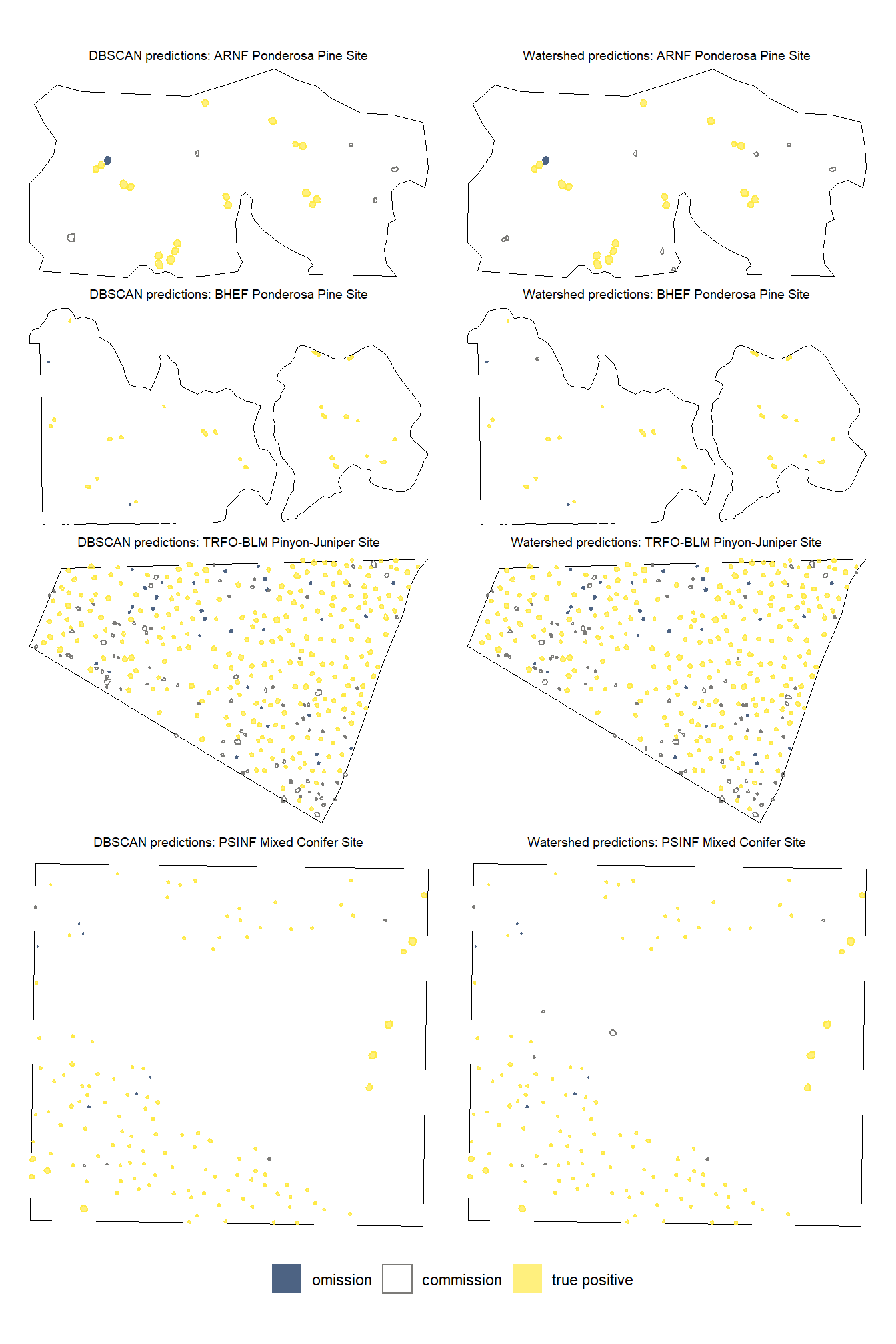

note the color legend…we like to see a lot of yellow :D

8.2 Detection Accuracy Metrics

now we aggregate the pile-level data (TP, FP, FN) into a single record for each study site and segmentation method combination. Detection performance metrics include F-score, precision, and recall.

8.2.1 Aggregate Instance Match Results

because our agg_ground_truth_match() function that we defined earlier includes capabilities to compute quantification metrics as well (e.g. height MAPE, RMSE, etc.), we’ll add the pile sizing metrics to our instance match data so that agg_ground_truth_match() recognizes them.

“diff_” columns are calculated as the predicted value minus the actual value (e.g. pred_diameter_m - gt_diameter_m)
“pct_diff_” columns are calculated as the actual value minus the predicted value divided by the actual value (e.g. (gt_diameter_m - pred_diameter_m)/gt_diameter_m)

# add prediction and validation measurements for dbscan
dbscan_gt_pred_match <- 
  dbscan_gt_pred_match %>% 
  purrr::imap(
    \(x,nm)
    # because psinf has field data but no others do
    if(nm=="psinf"){
      x %>% 
      # join on gt data
      dplyr::left_join(
        slash_piles_polys[[nm]] %>% 
          dplyr::rename(field_volume_m3=field_gt_volume_m3) %>% 
          dplyr::select(pile_id, image_gt_diameter_m, image_gt_area_m2, field_height_m, field_diameter_m, field_volume_m3) %>% 
          dplyr::rename_with(~ stringr::str_remove(.x, "^image_")) %>% 
          sf::st_drop_geometry()
        , by = "pile_id"
      ) %>% 
      # join on pred area data
      dplyr::left_join(
        dbscan_spectral_preds[[nm]] %>% 
          dplyr::select(
            pred_id
            , diameter_m
            , area_m2
            , volume_m3
            , max_height_m
          ) %>% 
          dplyr::rename(height_m=max_height_m) %>% 
          dplyr::rename_with(
            ~ paste0("pred_", .x, recycle0 = TRUE)
            , .cols = -c(pred_id)
          ) %>% 
          sf::st_drop_geometry()
        , by = "pred_id"
      ) %>% 
      # calculate difference columns
      dplyr::mutate(
        # area_m2
        diff_area_m2 = pred_area_m2-gt_area_m2
        , pct_diff_area_m2 = (gt_area_m2-pred_area_m2)/gt_area_m2
        # diameter_m
        , diff_diameter_m = pred_diameter_m-gt_diameter_m
        , pct_diff_diameter_m = (gt_diameter_m-pred_diameter_m)/gt_diameter_m
        # field diameter_m
        , diff_field_diameter_m = pred_diameter_m-field_diameter_m
        , pct_diff_field_diameter_m = (field_diameter_m-pred_diameter_m)/field_diameter_m
        # field height_m
        , diff_field_height_m = pred_height_m-field_height_m
        , pct_diff_field_height_m = (field_height_m-pred_height_m)/field_height_m
        # # field volume_m3
        # , diff_field_volume_m3 = pred_volume_m3-field_volume_m3
        # , pct_diff_field_volume_m3 = (field_volume_m3-pred_volume_m3)/field_volume_m3
      )  
    }else{
      x %>% 
      # join on gt data
      dplyr::left_join(
        slash_piles_polys[[nm]] %>% 
          dplyr::select(pile_id, image_gt_diameter_m, image_gt_area_m2) %>% 
          dplyr::rename_with(~ stringr::str_remove(.x, "^image_")) %>% 
          sf::st_drop_geometry()
        , by = "pile_id"
      ) %>% 
      # join on pred area data
      dplyr::left_join(
        dbscan_spectral_preds[[nm]] %>% 
          dplyr::select(
            pred_id
            , diameter_m
            , area_m2
            , volume_m3
            , max_height_m
          ) %>% 
          dplyr::rename(height_m=max_height_m) %>% 
          dplyr::rename_with(
            ~ paste0("pred_", .x, recycle0 = TRUE)
            , .cols = -c(pred_id)
          ) %>% 
          sf::st_drop_geometry()
        , by = "pred_id"
      ) %>% 
      # calculate difference columns
      dplyr::mutate(
        # area_m2
        diff_area_m2 = pred_area_m2-gt_area_m2
        , pct_diff_area_m2 = (gt_area_m2-pred_area_m2)/gt_area_m2
        # diameter_m
        , diff_diameter_m = pred_diameter_m-gt_diameter_m
        , pct_diff_diameter_m = (gt_diameter_m-pred_diameter_m)/gt_diameter_m
      )
    }
  )
# dbscan_gt_pred_match %>% dplyr::glimpse()
# add prediction and validation measurements for watershed
watershed_gt_pred_match <- 
  watershed_gt_pred_match %>% 
  purrr::imap(
    \(x,nm)
    # because psinf has field data but no others do
    if(nm=="psinf"){
      x %>% 
      # join on gt data
      dplyr::left_join(
        slash_piles_polys[[nm]] %>% 
          dplyr::rename(field_volume_m3=field_gt_volume_m3) %>% 
          dplyr::select(pile_id, image_gt_diameter_m, image_gt_area_m2, field_height_m, field_diameter_m, field_volume_m3) %>% 
          dplyr::rename_with(~ stringr::str_remove(.x, "^image_")) %>% 
          sf::st_drop_geometry()
        , by = "pile_id"
      ) %>% 
      # join on pred area data
      dplyr::left_join(
        watershed_spectral_preds[[nm]] %>% 
          dplyr::select(
            pred_id
            , diameter_m
            , area_m2
            , volume_m3
            , max_height_m
          ) %>% 
          dplyr::rename(height_m=max_height_m) %>% 
          dplyr::rename_with(
            ~ paste0("pred_", .x, recycle0 = TRUE)
            , .cols = -c(pred_id)
          ) %>% 
          sf::st_drop_geometry()
        , by = "pred_id"
      ) %>% 
      # calculate difference columns
      dplyr::mutate(
        # area_m2
        diff_area_m2 = pred_area_m2-gt_area_m2
        , pct_diff_area_m2 = (gt_area_m2-pred_area_m2)/gt_area_m2
        # diameter_m
        , diff_diameter_m = pred_diameter_m-gt_diameter_m
        , pct_diff_diameter_m = (gt_diameter_m-pred_diameter_m)/gt_diameter_m
        # field diameter_m
        , diff_field_diameter_m = pred_diameter_m-field_diameter_m
        , pct_diff_field_diameter_m = (field_diameter_m-pred_diameter_m)/field_diameter_m
        # field height_m
        , diff_field_height_m = pred_height_m-field_height_m
        , pct_diff_field_height_m = (field_height_m-pred_height_m)/field_height_m
        # # field volume_m3
        # , diff_field_volume_m3 = pred_volume_m3-field_volume_m3
        # , pct_diff_field_volume_m3 = (field_volume_m3-pred_volume_m3)/field_volume_m3
      )  
    }else{
      x %>% 
      # join on gt data
      dplyr::left_join(
        slash_piles_polys[[nm]] %>% 
          dplyr::select(pile_id, image_gt_diameter_m, image_gt_area_m2) %>% 
          dplyr::rename_with(~ stringr::str_remove(.x, "^image_")) %>% 
          sf::st_drop_geometry()
        , by = "pile_id"
      ) %>% 
      # join on pred area data
      dplyr::left_join(
        watershed_spectral_preds[[nm]] %>% 
          dplyr::select(
            pred_id
            , diameter_m
            , area_m2
            , volume_m3
            , max_height_m
          ) %>% 
          dplyr::rename(height_m=max_height_m) %>% 
          dplyr::rename_with(
            ~ paste0("pred_", .x, recycle0 = TRUE)
            , .cols = -c(pred_id)
          ) %>% 
          sf::st_drop_geometry()
        , by = "pred_id"
      ) %>% 
      # calculate difference columns
      dplyr::mutate(
        # area_m2
        diff_area_m2 = pred_area_m2-gt_area_m2
        , pct_diff_area_m2 = (gt_area_m2-pred_area_m2)/gt_area_m2
        # diameter_m
        , diff_diameter_m = pred_diameter_m-gt_diameter_m
        , pct_diff_diameter_m = (gt_diameter_m-pred_diameter_m)/gt_diameter_m
      )
    }
  )
# watershed_gt_pred_match %>% dplyr::glimpse()
# agg_ground_truth_match(watershed_gt_pred_match[[1]]) %>% dplyr::glimpse()
# watershed_gt_pred_match[["pj"]] %>% dplyr::count(pred_id) %>% dplyr::filter(n>1) %>% dplyr::arrange(desc(n))
# dbscan_gt_pred_match[["pj"]] %>% dplyr::count(pred_id) %>% dplyr::filter(n>1) %>% dplyr::arrange(desc(n))

apply our agg_ground_truth_match() function

agg_ground_truth_match_ans <- 
  dplyr::bind_rows(
    dbscan_gt_pred_match %>% 
      purrr::map_dfr(agg_ground_truth_match, .id = "site_data_lab") %>% 
      dplyr::mutate(method = "dbscan") %>% 
      dplyr::bind_rows()
    , watershed_gt_pred_match %>% 
      purrr::map_dfr(agg_ground_truth_match, .id = "site_data_lab") %>% 
      dplyr::mutate(method = "watershed") %>% 
      dplyr::bind_rows()
  ) %>% 
  dplyr::inner_join(
    all_stand_boundary %>% 
      dplyr::select(site_data_lab, site, site_full_lab) %>% 
      sf::st_drop_geometry()
    , by = "site_data_lab"
  ) %>% 
  # make factor
  dplyr::mutate(
    site = ordered(site)
    , site_full_lab = ordered(site_full_lab)
    , method = method %>%
      factor(ordered = T) %>% 
      forcats::fct_recode("DBSCAN" = "dbscan", "Watershed" = "watershed")
  )

what did we get?

agg_ground_truth_match_ans %>% 
  dplyr::glimpse()

## Rows: 8
## Columns: 24
## $ site_data_lab                  <chr> "arnf", "bhef", "psinf", "pj", "arnf", …
## $ tp_n                           <dbl> 18, 24, 115, 245, 18, 24, 115, 245
## $ fp_n                           <dbl> 5, 0, 5, 85, 8, 1, 8, 84
## $ fn_n                           <dbl> 1, 2, 6, 31, 1, 2, 6, 31
## $ omission_rate                  <dbl> 0.05263158, 0.07692308, 0.04958678, 0.1…
## $ commission_rate                <dbl> 0.21739130, 0.00000000, 0.04166667, 0.2…
## $ precision                      <dbl> 0.7826087, 1.0000000, 0.9583333, 0.7424…
## $ recall                         <dbl> 0.9473684, 0.9230769, 0.9504132, 0.8876…
## $ f_score                        <dbl> 0.8571429, 0.9600000, 0.9543568, 0.8085…
## $ diff_area_m2_rmse              <dbl> 16.594443, 48.389761, 2.050426, 1.74660…
## $ diff_diameter_m_rmse           <dbl> 0.6451003, 2.4203931, 0.3832957, 0.3879…
## $ diff_area_m2_mean              <dbl> 12.7587200, -24.8476306, -0.7831500, -0…
## $ diff_diameter_m_mean           <dbl> -0.4015052, -1.3737463, -0.2049347, -0.…
## $ pct_diff_area_m2_mape          <dbl> 0.03548836, 0.14870735, 0.10290712, 0.1…
## $ pct_diff_diameter_m_mape       <dbl> 0.01779425, 0.08146903, 0.06780040, 0.0…
## $ diff_field_diameter_m_rmse     <dbl> NA, NA, 0.4664407, NA, NA, NA, 0.471317…
## $ diff_field_height_m_rmse       <dbl> NA, NA, 0.6679947, NA, NA, NA, 0.667994…
## $ diff_field_diameter_m_mean     <dbl> NA, NA, 0.1892385, NA, NA, NA, 0.192082…
## $ diff_field_height_m_mean       <dbl> NA, NA, -0.06963052, NA, NA, NA, -0.069…
## $ pct_diff_field_diameter_m_mape <dbl> NA, NA, 0.1000518, NA, NA, NA, 0.101088…
## $ pct_diff_field_height_m_mape   <dbl> NA, NA, 0.1916669, NA, NA, NA, 0.191666…
## $ method                         <ord> DBSCAN, DBSCAN, DBSCAN, DBSCAN, Watersh…
## $ site                           <ord> ARNF Ponderosa Pine Site, BHEF Ponderos…
## $ site_full_lab                  <ord> Arapahoe and Roosevelt National Forest …

8.2.2 Detection Accuracy Results

let’s make a nice table of the detection accuracy metrics by study site and segmentation method

agg_ground_truth_match_ans %>% 
  dplyr::select(
    site, method
    , tidyselect::ends_with("_n")
    , precision, recall, f_score
  ) %>% 
  dplyr::mutate(
    dplyr::across(
      tidyselect::ends_with("_n")
      , ~scales::comma(.x,accuracy=1)
    )
    , dplyr::across(
      dplyr::where(is.numeric)
      , ~scales::percent(.x,accuracy=0.1)
    )
  ) %>% 
  dplyr::arrange(site,method) %>% 
  kableExtra::kbl(
    caption = "Detection Accuracy"
    , col.names = c(
      "site", "method"
      , "TP predictions", "FP predictions", "FN predictions"
      , "Precision", "Recall", "F-score"
    )
    , escape = F
    # , digits = 2
  ) %>% 
  kableExtra::kable_styling() %>% 
  kableExtra::collapse_rows(columns = 1, valign = "top")

Table 8.2: Detection Accuracy
site	method	TP predictions	FP predictions	FN predictions	Precision	Recall	F-score
ARNF Ponderosa Pine Site	DBSCAN	18	5	1	78.3%	94.7%	85.7%
ARNF Ponderosa Pine Site	Watershed	18	8	1	69.2%	94.7%	80.0%
BHEF Ponderosa Pine Site	DBSCAN	24	0	2	100.0%	92.3%	96.0%
BHEF Ponderosa Pine Site	Watershed	24	1	2	96.0%	92.3%	94.1%
PSINF Mixed Conifer Site	DBSCAN	115	5	6	95.8%	95.0%	95.4%
PSINF Mixed Conifer Site	Watershed	115	8	6	93.5%	95.0%	94.3%
TRFO-BLM Pinyon-Juniper Site	DBSCAN	245	85	31	74.2%	88.8%	80.9%
TRFO-BLM Pinyon-Juniper Site	Watershed	245	84	31	74.5%	88.8%	81.0%

8.3 Segmentation Method Accuracy Comparison

Our slash pile detection methodology implements and tests two different segmentation approaches to identify candidate slash piles from the CHM. We fully reviewed these two approaches here but we’ll present a quick review. First, the watershed segmentation method is a raster-based technique that treats the inverted height surface as a topographic landscape where local maxima serve as initial seeds to define the boundaries of individual basins. Second, DBSCAN segmentation is traditionally a point-based clustering method that we adapted for raster data by treating the cell centroids as points. To maintain consistency across varying datasets and limit the amount of effort required by users, we developed a dynamic parameterization logic that automatically calibrates both algorithms by translating user-defined physical dimensions into data-specific values. This dynamic parameterization uses the target pile size and input data resolution to calculate geometry-based search windows and density thresholds to ensure that the algorithm settings are proportional to the target object regardless of changes in input data resolution.

let’s make some plots to visualize this information

agg_ground_truth_match_ans %>% 
  dplyr::select(
    site, method
    , precision, recall, f_score
  ) %>% 
  tidyr::pivot_longer(
    cols = c(precision,recall,f_score)
    , names_to = "metric"
    , values_to = "value"
  ) %>% 
  dplyr::mutate(
    metric = metric %>%
      forcats::fct_relevel("f_score", "recall", "precision") %>%
      forcats::fct_recode("F-score" = "f_score", "Recall" = "recall", "Precision" = "precision")
  ) %>% 
  dplyr::mutate(
    dplyr::across(
      dplyr::where(is.numeric)
      , list(lab = ~scales::percent(.x,accuracy=0.1))
    )
  ) %>% 
  dplyr::mutate(site = stringr::word(site)) %>% 
  # dplyr::pull(metric) %>% levels()
  ggplot2::ggplot(
    mapping = ggplot2::aes(
      y = value, x = method
      , color = metric, group = metric
    )
  ) +
  ggplot2::geom_line(alpha = 0.8, lwd = 2) +
   # lhs labs
  ggrepel::geom_text_repel(
    data = function(x){dplyr::filter(x,method == "DBSCAN")}
    , mapping = ggplot2::aes(label = value_lab, fontface = "bold")
    # , color = "black"
    , size = 3
    # , min.segment.length = 0
    , nudge_x = -0.1
    , direction = "y"
    , hjust = 1
  ) +
  # rhs labs
  ggrepel::geom_text_repel(
    data = function(x){dplyr::filter(x,method == "Watershed")}
    , mapping = ggplot2::aes(label = value_lab, fontface = "bold")
    # , color = "black"
    , size = 3
    # , min.segment.length = 0
    , nudge_x = 0.1
    , direction = "y"
    , hjust = 0
  ) +
  ggplot2::geom_point(size = 3) +
  ggplot2::scale_color_manual(values=pal_eval_metric2) +
  ggplot2::scale_y_continuous(
    limits = c(0,1)
    , labels=scales::percent
    , breaks = scales::breaks_extended(n=6)
    , expand = ggplot2::expansion(mult = c(0,0.03))
  ) +
  ggplot2::facet_grid(
    cols = dplyr::vars(site)
    , axes = "all"
  ) +
  ggplot2::labs(
    color="",x="Segmentation Method",y=""
  ) +
  ggplot2::theme_light() +
  ggplot2::theme(
    legend.position = "top"
    , strip.text = ggplot2::element_text(size = 10, color = "black", face = "bold")
    , axis.text.x = ggplot2::element_text(size = 10)
  ) +
  ggplot2::guides(
    color = ggplot2::guide_legend(override.aes = list(shape = 15, linetype = 0, size = 6, alpha = 1))
  )

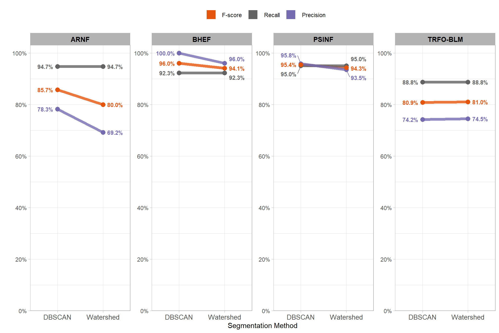
recall never changes, the changes in F-score are entirely due to changes in precision

8.3.1 Paired T-Test

To compare the detection performance of the two algorithms across our set of four study sites, we can quickly use a paired t-test to check if the average of the differences in F-score between the two methods is significantly different from zero. If the p-value is less than 0.05, you can say the difference is statistically significant. However, with only four sites this test may not be robust enough to detect differences in detection accuracy across the methods unless one method is a lot better…

# get scores for each method since t.test needs the sites to be ORDERED the same for proper "paired" comparison
dbscan_temp <- agg_ground_truth_match_ans %>% 
  dplyr::arrange(site) %>% 
  dplyr::filter(tolower(method) == "dbscan") %>% 
  dplyr::pull(f_score)
watershed_temp <- agg_ground_truth_match_ans %>% 
  dplyr::arrange(site) %>% 
  dplyr::filter(tolower(method) == "watershed") %>% 
  dplyr::pull(f_score)
# t.test
ttest_temp <- t.test(dbscan_temp, watershed_temp, paired = T)

let’s see what we got

ttest_temp

## 
##  Paired t-test
## 
## data:  dbscan_temp and watershed_temp
## t = 1.7184, df = 3, p-value = 0.1842
## alternative hypothesis: true mean difference is not equal to 0
## 95 percent confidence interval:
##  -0.01839518  0.06157707
## sample estimates:
## mean difference 
##      0.02159095

the t.test() computed the mean difference (MD) between the DBSCAN and Watershed F-score to determine if the difference is statistically significant (i.e. significantly different from zero). the mean difference (MD) is 2.16% (DBSCAN F-Score minus Watershed F-Score). the p-value of 0.1842 is greater than 0.05, meaning we fail to reject the null hypothesis that the true mean difference is zero. this implies that neither the DBSCAN nor the Watershed method was statistically significantly better (or worse) than the other segmentation method at correctly identifying the location of actual slash piles while minimizing incorrect predictions at locations where no actual pile was present.

8.3.2 Bayesian Approach

The paired t-test above failed to detect a difference in detection accuracy (F-score) by segmentation method (DBSCAN vs Watershed). With only four sites the paired t-test may not be robust enough to detect differences in detection accuracy across the methods. An alternative is a quick Bayesian model which may provide a more robust alternative to the paired t-test by estimating the full probability distribution of the difference between methods rather than relying on a single p-value. While a paired t-test simply evaluates the average difference within sites, a Bayesian model can account for the nested structure of the data by allowing the intercept to vary by study site ((1|site) in the model) while keeping the slope constant across locations (f_score ~ method in the model). The slope of the model represents the effect of the segmentation method. This approach allows the model to adjust for the unique baseline difficulty of pile detection at each study site and isolates the detection accuracy change caused by using a different segmentation method. Since F-score is bound between zero and one, we use a Beta regression family to ensure predictions are not made outside of these bounds.

The fully-factored model specification:

\[ \begin{aligned} \text{Likelihood:} \\ y_{i} &\sim \text{Beta}(\mu_{i}, \phi) \\ \\ \text{Linear Predictor:} \\ \text{logit}(\mu_{i}) &= \alpha + \alpha_{\text{site}[i]} + \beta \cdot \text{Method}_{i} \\ \\ \text{Priors:} \\ \alpha &\sim \text{Student-t}(3, 0, 2.5) \\ \beta &\sim \text{Normal}(0, 1) \\ \alpha_{\text{site}} &\sim \text{Normal}(0, \sigma_{\text{site}}) \\ \sigma_{\text{site}} &\sim \text{Student-t}(3, 0, 2.5) \\ \phi &\sim \text{Gamma}(0.01, 0.01) \end{aligned} \]

where, \(y_{i}\) represents the F-score for the \(i\)-th observation within study site \(j\), parameterized using the mean \(\mu\) and a precision parameter \(\phi\)

# brms::brm
fscore_mod_method_temp <- brms::brm(
  f_score ~ method + (1|site)
  , data = agg_ground_truth_match_ans
  # family
  , family = brms::Beta(link = "logit")
  # mcmc
  , iter = 20000, warmup = 10000
  # , iter = 6000, warmup = 3000
  , chains = 4
  , cores = lasR::half_cores()
  , file = paste0("../data/", "fscore_mod_seg_method")
  # , file = paste0("../data/", "fscore_mod_method")
  , control = list(adapt_delta = 0.999, max_treedepth = 13)
)
# look at results
# plot(fscore_mod_method_temp)
# summary(fscore_mod_method_temp)
# check the prior distributions
# check priors
# brms::prior_summary(fscore_mod_method_temp) %>%
#   kableExtra::kbl() %>% 
#   kableExtra::kable_styling()

8.3.2.1 Posterior Predictive Checks

check the trace plots for problems with convergence of the Markov chains

plot(fscore_mod_method_temp)

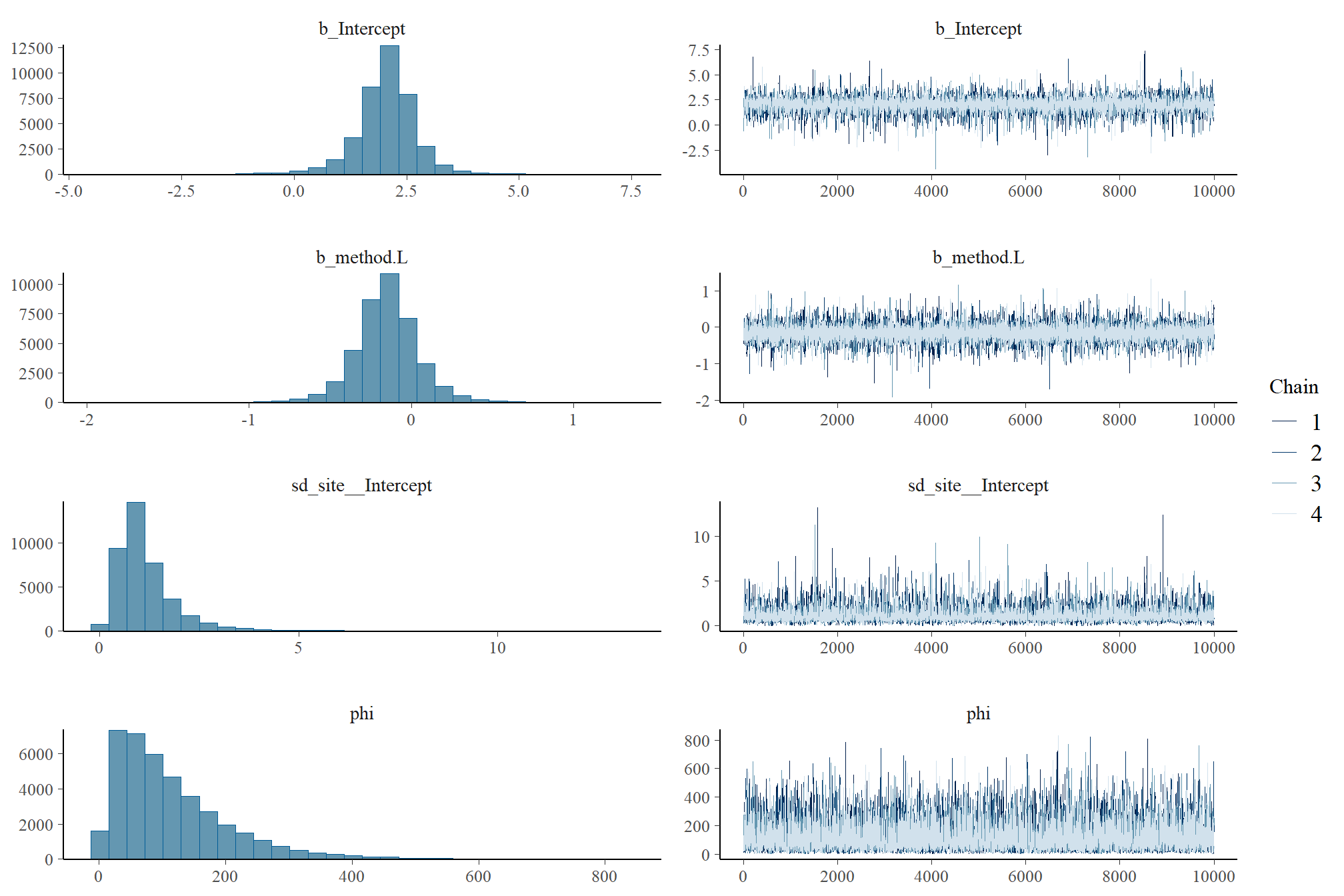
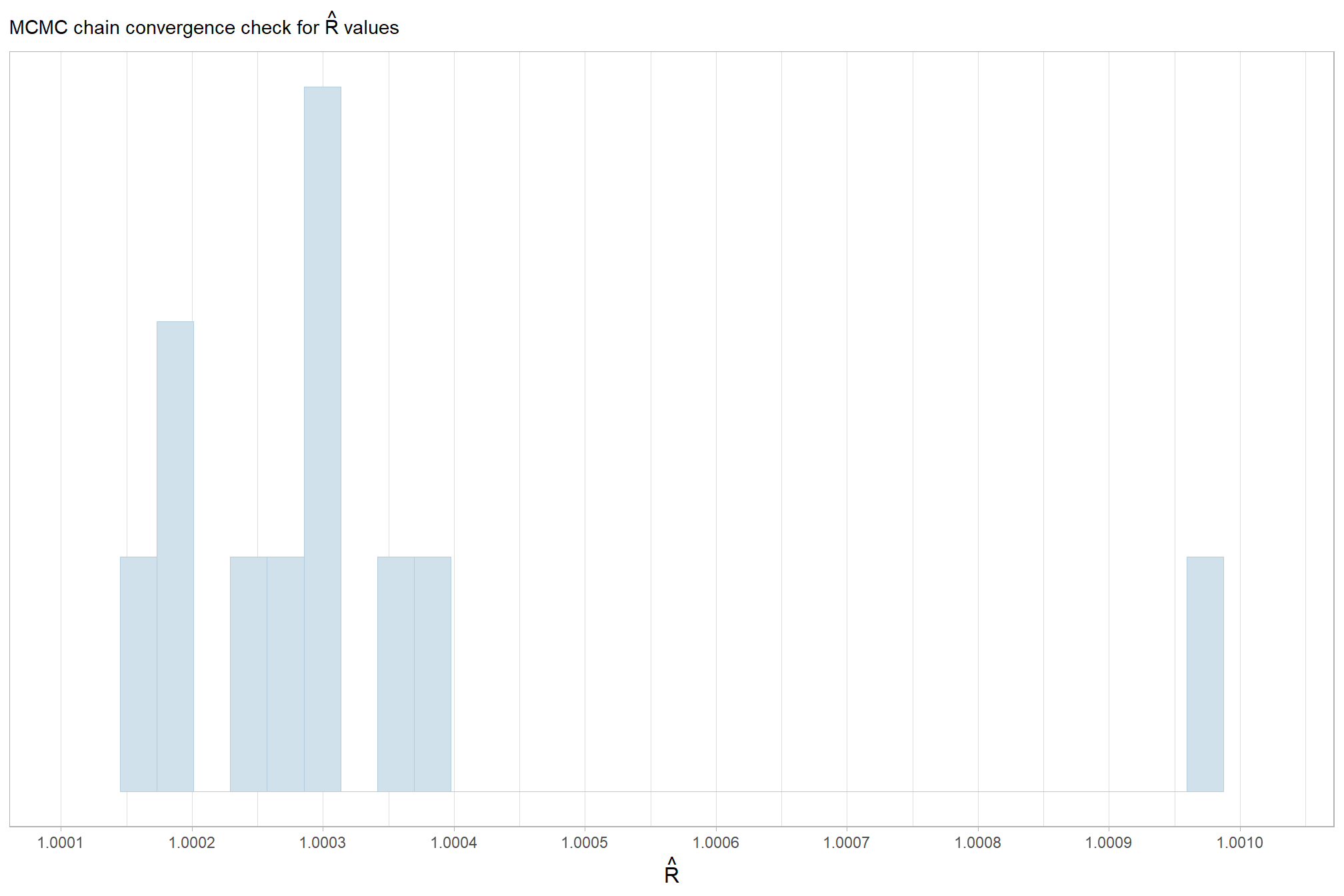
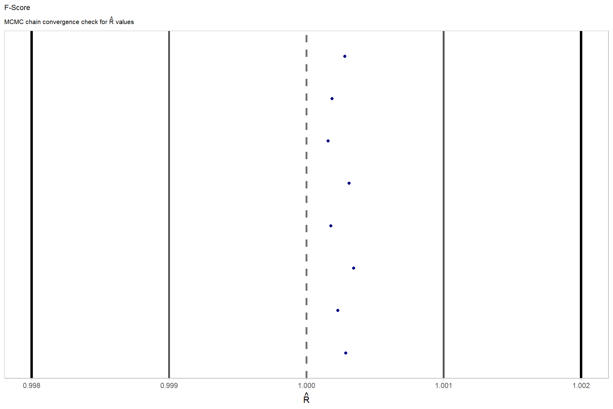
Sufficient convergence was checked with \(\hat{R}\) values near 1 (Brooks & Gelman, 1998).

in the plot below, \(\hat{R}\) values are colored using different shades (lighter is better). The chosen thresholds are somewhat arbitrary, but can be useful guidelines in practice (Gabry and Mahr 2025):

light: below 1.05 (good)
mid: between 1.05 and 1.1 (ok)
dark: above 1.1 (too high)

check our \(\hat{R}\) values

brms::mcmc_plot(fscore_mod_method_temp, type = "rhat_hist") +
  ggplot2::scale_x_continuous(breaks = scales::breaks_extended(n = 8), expand = ggplot2::expansion(mult = c(0.1,0.1))) +
  ggplot2::scale_y_continuous(NULL, breaks = NULL) +
  ggplot2::labs(
    subtitle = latex2exp::TeX("MCMC chain convergence check for $\\hat{R}$ values")
  ) +
  ggplot2::theme_light() +
  ggplot2::theme(
    legend.position = "none"
    , legend.direction = "horizontal"
    , plot.subtitle = ggplot2::element_text()
    , axis.title.x = ggplot2::element_text(size = 12)
  )

ggplot2::ggsave("../data/bayes_mcmc_chk1.jpeg", height = 7, width = 8.5, dpi = 300)

and another check of our \(\hat{R}\) values

# and another check of our $\hat{R}$ values
fscore_mod_method_temp %>% 
  brms::rhat() %>% 
  as.data.frame() %>% 
  tibble::rownames_to_column(var = "parameter") %>%
  dplyr::rename_with(tolower) %>% 
  dplyr::rename(rhat = 2) %>% 
  dplyr::filter(
    stringr::str_starts(parameter, "b_") 
    | stringr::str_starts(parameter, "r_") 
    | stringr::str_starts(parameter, "sd_") 
    | parameter == "phi"
  ) %>%
  dplyr::mutate(
    chk = (rhat <= 1*0.998 | rhat >= 1*1.002)
  ) %>% 
  ggplot2::ggplot(ggplot2::aes(x = rhat, y = parameter, color = chk, fill = chk)) +
  ggplot2::geom_vline(xintercept = 1, linetype = "dashed", color = "gray44", lwd = 1.2) +
  ggplot2::geom_vline(xintercept = 1*0.998, lwd = 1.5) +
  ggplot2::geom_vline(xintercept = 1*1.002, lwd = 1.5) +
  ggplot2::geom_vline(xintercept = 1*0.999, lwd = 1.2, color = "gray33") +
  ggplot2::geom_vline(xintercept = 1*1.001, lwd = 1.2, color = "gray33") +
  ggplot2::geom_point() +
  ggplot2::scale_fill_manual(values = c("navy", "firebrick")) +
  ggplot2::scale_color_manual(values = c("navy", "firebrick")) +
  ggplot2::scale_y_discrete(NULL, breaks = NULL) +
  ggplot2::labs(
    x = latex2exp::TeX("$\\hat{R}$")
    , subtitle = latex2exp::TeX("MCMC chain convergence check for $\\hat{R}$ values")
    , title = "F-Score"
  ) +
  ggplot2::theme_light() +
  ggplot2::theme(
    legend.position = "none"
    , axis.text.y = ggplot2::element_text(size = 4)
    , panel.grid.major.x = ggplot2::element_blank()
    , panel.grid.minor.x = ggplot2::element_blank()
    , plot.subtitle = ggplot2::element_text(size = 8)
    , plot.title = ggplot2::element_text(size = 9)
  )

The effective length of an MCMC chain is indicated by the effective sample size (ESS), which refers to the sample size of the MCMC chain not to the sample size of the data where acceptable values allow “for reasonably accurate and stable estimates of the limits of the 95% HDI…If accuracy of the HDI limits is not crucial for your application, then a smaller ESS may be sufficient” (Kruschke 2015, p. 184)

Ratios of effective sample size (ESS) to total sample size with values are colored using different shades (lighter is better). A ratio close to “1” (no autocorrelation) is ideal, while a low ratio suggests the need for more samples or model re-parameterization. Efficiently mixing MCMC chains are important because they guarantee the resulting posterior samples accurately represent the true distribution of model parameters, which is necessary for reliable and precise estimation of parameter values and their associated uncertainties (credible intervals). The chosen thresholds are somewhat arbitrary, but can be useful guidelines in practice (Gabry and Mahr 2025):

light: between 0.5 and 1 (high)
mid: between 0.1 and 0.5 (good)
dark: below 0.1 (low)

# and another effective sample size check
brms::mcmc_plot(fscore_mod_method_temp, type = "neff_hist") +
# brms::mcmc_plot(fscore_mod_method_temp, type = "neff") +
  ggplot2::scale_x_continuous(limits = c(0,NA), breaks = scales::breaks_extended(n = 9)) +
  ggplot2::scale_y_continuous(NULL, breaks = NULL) +
  ggplot2::labs(
    subtitle = "MCMC chain resolution check for effective sample size (ESS) ratios"
  ) +
  ggplot2::theme_light() +
  ggplot2::theme(
    legend.position = "none"
    , legend.direction = "horizontal"
    , plot.subtitle = ggplot2::element_text()
    , axis.title.x = ggplot2::element_text(size = 12)
  )

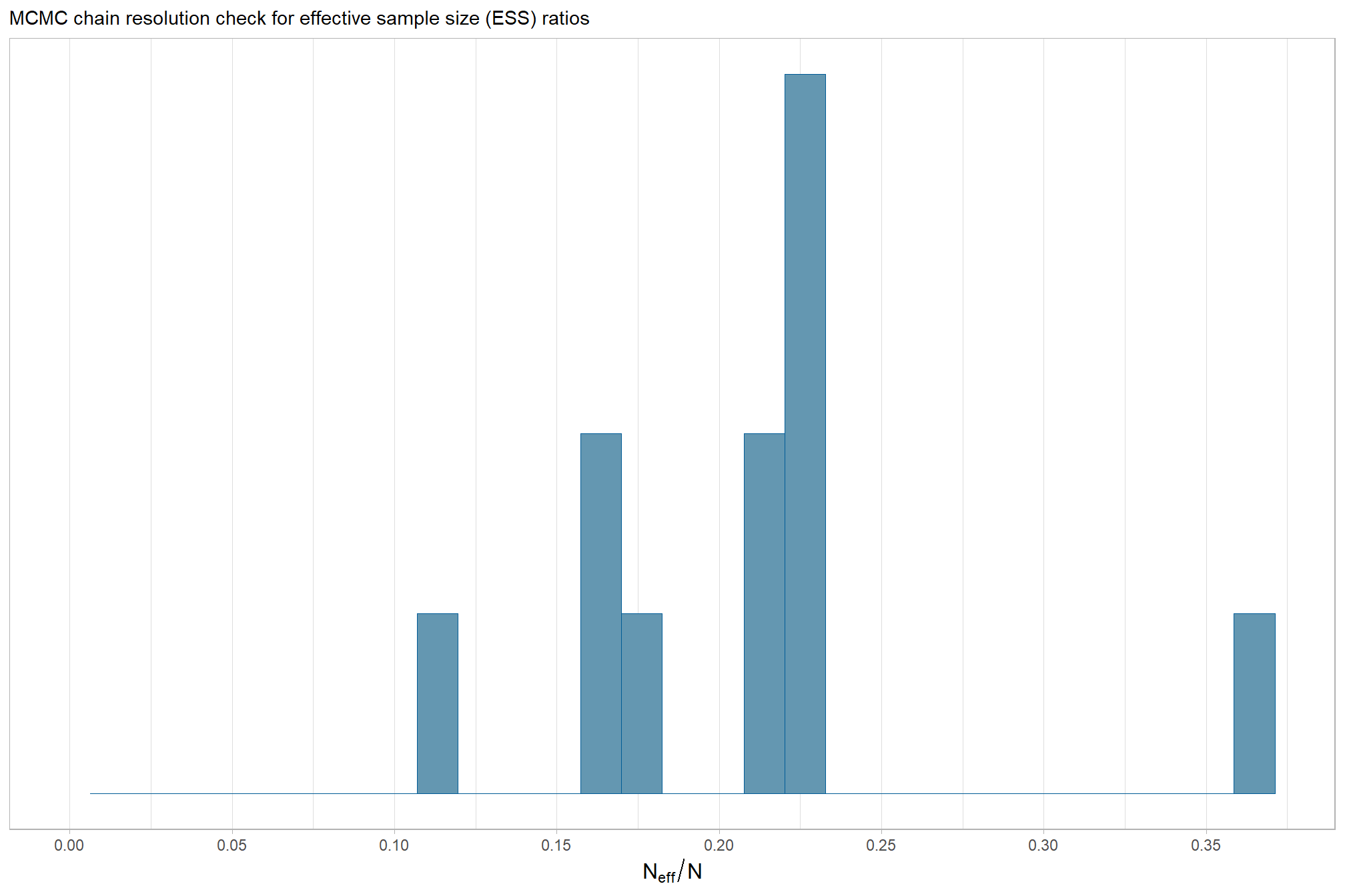
ggplot2::ggsave("../data/bayes_mcmc_chk2.jpeg", height = 7, width = 8.5, dpi = 300)

our observed range of ESS to Total Sample Size ratios are generally considered good to excellent, indicating the MCMC chains are performing well and mixing efficiently

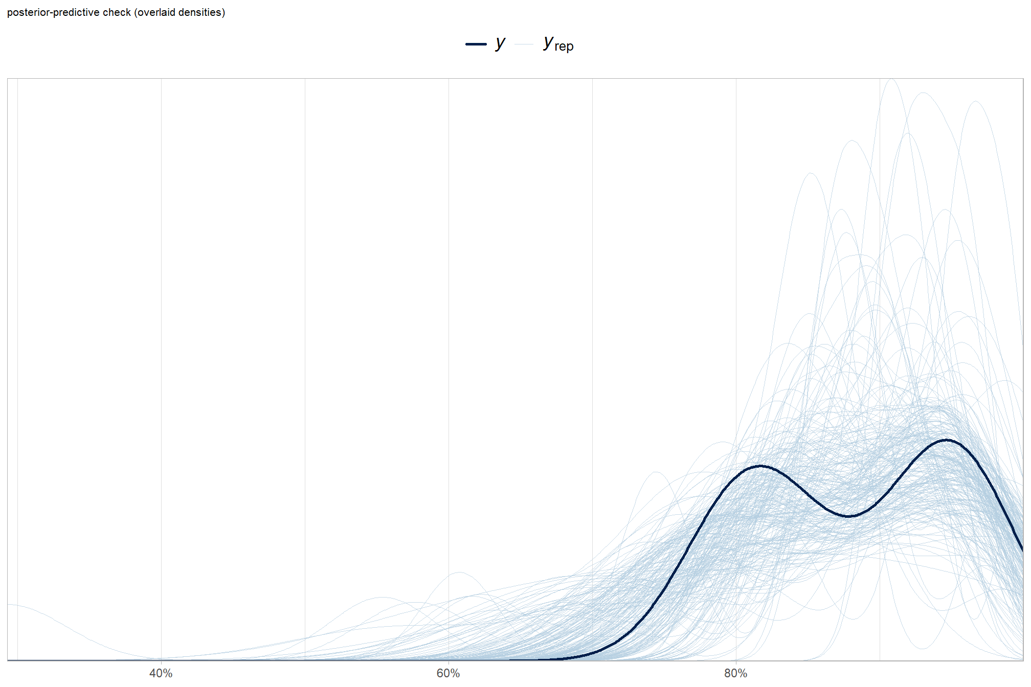
Posterior predictive checks were used to evaluate model goodness-of-fit by comparing data simulated from the model with the observed data used to estimate the model parameters (Hobbs & Hooten, 2015).

To learn more about this approach to posterior predictive checks, check out Gabry’s (2025) vignette, Graphical posterior predictive checks using the bayesplot package.

posterior-predictive check to make sure the model does an okay job simulating data that resemble the sample data. our objective is to construct the model such that it faithfully represents the data.

8.3.2.1.1 Overall

# posterior predictive check
brms::pp_check(
    fscore_mod_method_temp
    , type = "dens_overlay"
    , ndraws = 222
  ) + 
  ggplot2::labs(subtitle = "posterior-predictive check (overlaid densities)") +
  ggplot2::theme_light() +
  ggplot2::scale_y_continuous(NULL, breaks = NULL) +
  ggplot2::scale_x_continuous(labels=scales::percent) +
  ggplot2::theme(
    legend.position = "top", legend.direction = "horizontal"
    , legend.text = ggplot2::element_text(size = 14)
    , plot.subtitle = ggplot2::element_text(size = 8)
    , plot.title = ggplot2::element_text(size = 9)
  )

and another posterior predictive check for the overall model combining mean and sd

# brms::pp_check(fscore_mod_method_temp, type = "xxx")
# and another posterior predictive check for the overall model combining mean and sd
set.seed(77)
p1_temp <-
  brms::pp_check(
    fscore_mod_method_temp
    , type = "stat_2d"
    , stat = c("median","sd")
    , ndraws = 4444
  ) +
  ggplot2::theme_light() +
  ggplot2::scale_x_continuous(labels=scales::percent) +
  ggplot2::labs(
    subtitle = "(a) Overall joint distribution of F-score median and SD"
    , x = "F-score median"
  ) +
  ggplot2::theme(
    legend.position = "top", legend.direction = "horizontal"
    , legend.text = ggplot2::element_text(size = 8)
    , legend.title = ggplot2::element_blank()
    , plot.subtitle = ggplot2::element_text(face = "bold")
    , strip.text = ggplot2::element_text(face = "bold", color = "black")
  ) +
  ggplot2::guides(
    color = ggplot2::guide_legend(
      override.aes = list(shape = 15, size = 8, linetype = 0)
    )
  )
p1_temp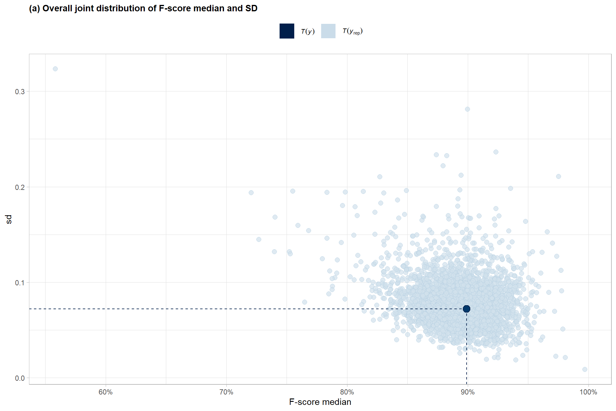

overall median

set.seed(55)
p8_temp <- 
  brms::pp_check(
    fscore_mod_method_temp
    , type = "stat"
    , stat = "median"
    , ndraws = 888
  ) +
  ggplot2::theme_light() +
  ggplot2::scale_y_continuous(NULL, breaks = NULL) +
  ggplot2::scale_x_continuous(labels=scales::percent) +
  ggplot2::labs(
    subtitle = "(b) Overall distribution of simulated F-score median"
    , x = "F-score median"
  ) +
  ggplot2::theme(
    legend.position = "top", legend.direction = "horizontal"
    , legend.text = ggplot2::element_text(size = 8)
    , legend.title = ggplot2::element_blank()
    , plot.subtitle = ggplot2::element_text(face = "bold")
    , strip.text = ggplot2::element_text(face = "bold", color = "black")
  )
p8_temp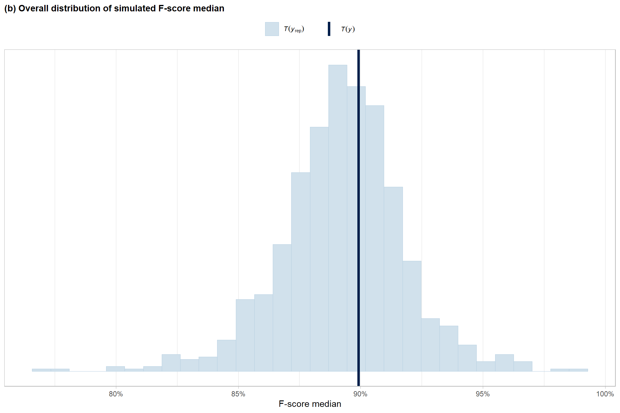

8.3.2.1.2 Grouped

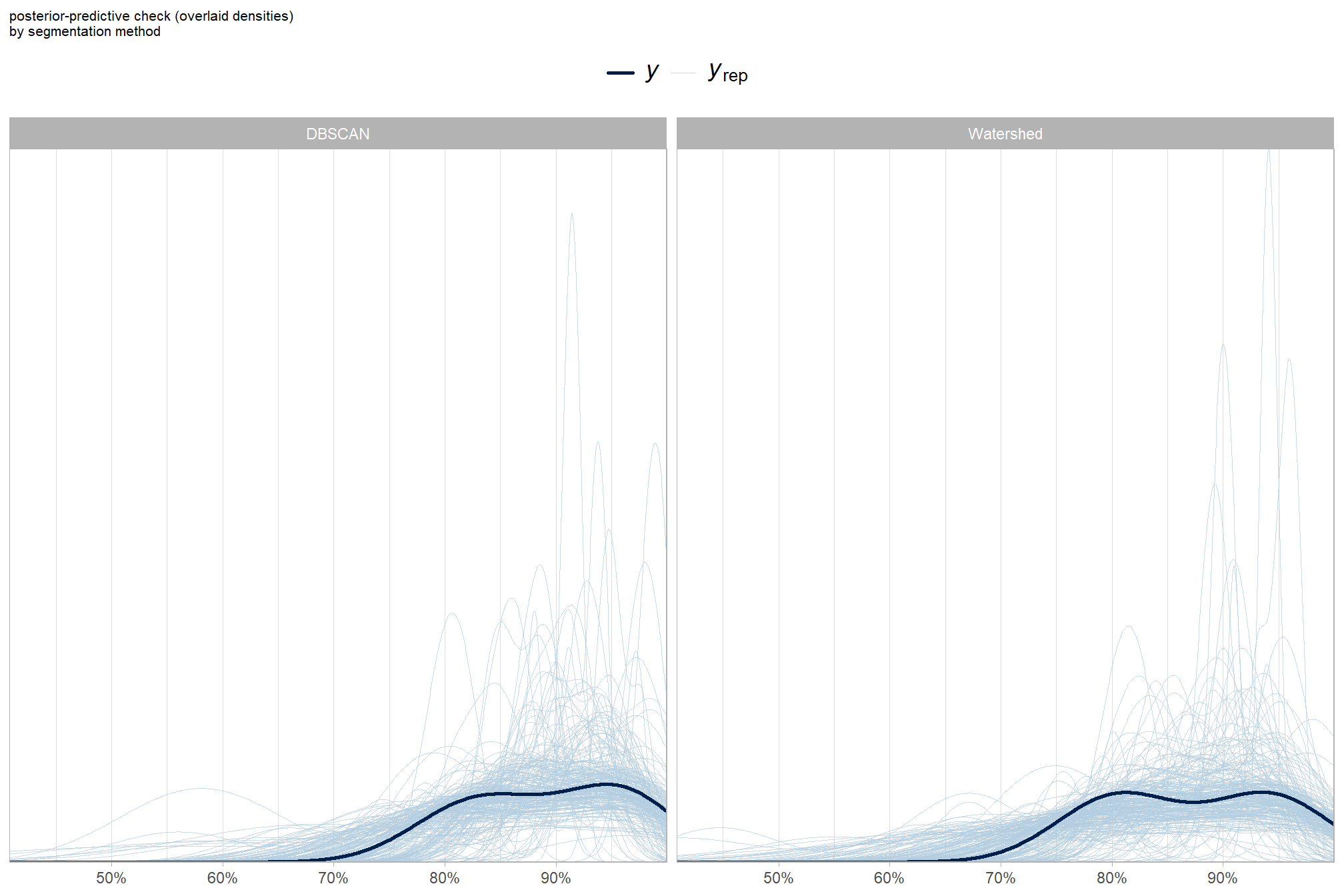
grouped density overlay by method

brms::pp_check(
    fscore_mod_method_temp
    , type = "dens_overlay_grouped" # ""
    , group = "method"
    , ndraws = 222
  ) + 
  ggplot2::labs(subtitle = "posterior-predictive check (overlaid densities)\nby segmentation method") +
  ggplot2::theme_light() +
  ggplot2::scale_y_continuous(NULL, breaks = NULL) +
  ggplot2::scale_x_continuous(labels=scales::percent) +
  ggplot2::theme(
    legend.position = "top", legend.direction = "horizontal"
    , legend.text = ggplot2::element_text(size = 14)
    , plot.subtitle = ggplot2::element_text(size = 8)
    , plot.title = ggplot2::element_text(size = 9)
  )

grouped median by method

# grouped
p2_temp <-
  brms::pp_check(
    fscore_mod_method_temp
    , type = "stat_grouped" # "dens_overlay_grouped"
    , stat = "median"
    , group = "method"
    , ndraws = 888
  ) + 
  ggplot2::theme_light() +
  ggplot2::scale_y_continuous(NULL, breaks = NULL) +
  ggplot2::scale_x_continuous(labels=scales::percent) +
  ggplot2::labs(
    subtitle = "(c) Distribution of simulated F-score median by segmentation method"
    , x = "F-score median"
  ) +
  ggplot2::theme(
    legend.position = "top", legend.direction = "horizontal"
    , legend.text = ggplot2::element_text(size = 8)
    , plot.subtitle = ggplot2::element_text(face = "bold")
    , strip.text = ggplot2::element_text(face = "bold", color = "black")
  )
# p2_temp
# p2_temp$facet
# p2_temp$facet$params$facets
p2_temp <- 
  p2_temp +
  ggplot2::facet_wrap(
    facets = p2_temp$facet$params$facets
    # , ncol = 1
    , scales = "free_y"
  )
p2_temp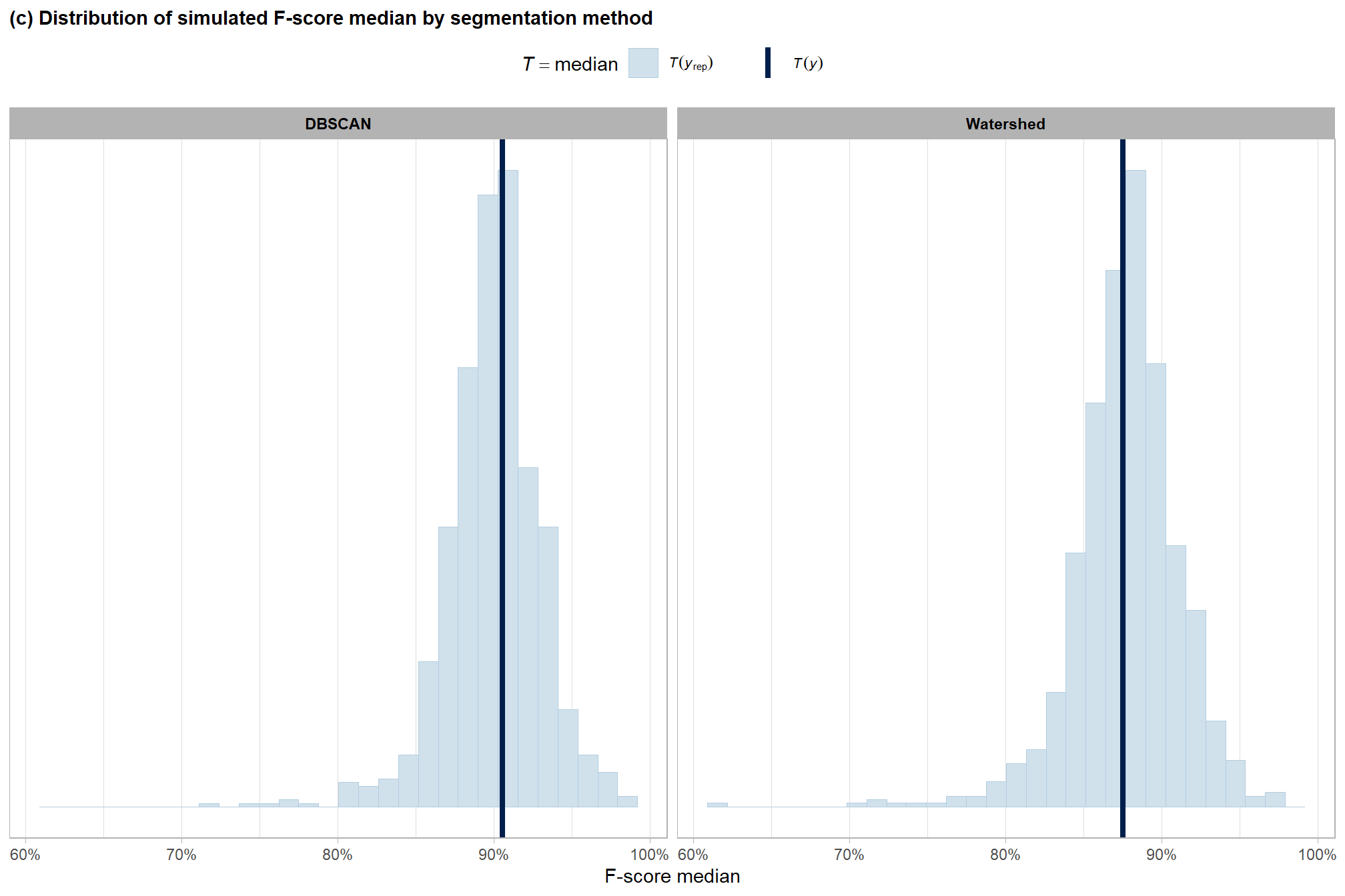

grouped median by site

# grouped
p3_temp <-
  brms::pp_check(
    fscore_mod_method_temp
    , type = "stat_grouped" # "dens_overlay_grouped"
    , stat = "median"
    , group = "site"
    , ndraws = 888
  ) + 
  ggplot2::theme_light() +
  ggplot2::scale_y_continuous(NULL, breaks = NULL) +
  ggplot2::scale_x_continuous(labels=scales::percent) +
  ggplot2::labs(
    subtitle = "(d) Distribution of simulated F-score median by site"
    , x = "F-score median"
  ) +
  ggplot2::theme(
    legend.position = "top", legend.direction = "horizontal"
    , legend.text = ggplot2::element_text(size = 8)
    , plot.subtitle = ggplot2::element_text(face = "bold")
    , strip.text = ggplot2::element_text(face = "bold", color = "black")
  )
# p3_temp
# p3_temp$facet
# p3_temp$facet$params$facets
p3_temp <- 
  p3_temp +
  ggplot2::facet_wrap(
    facets = p3_temp$facet$params$facets
    , nrow = 1
    , labeller = 
      ggplot2::as_labeller(function(x) gsub(" .*", "", x))
      # ggplot2::as_labeller(
      #   setNames(unique(agg_ground_truth_match_ans$site_full_lab), unique(agg_ground_truth_match_ans$site))
      # )
    , scales = "free_y"
  )
p3_temp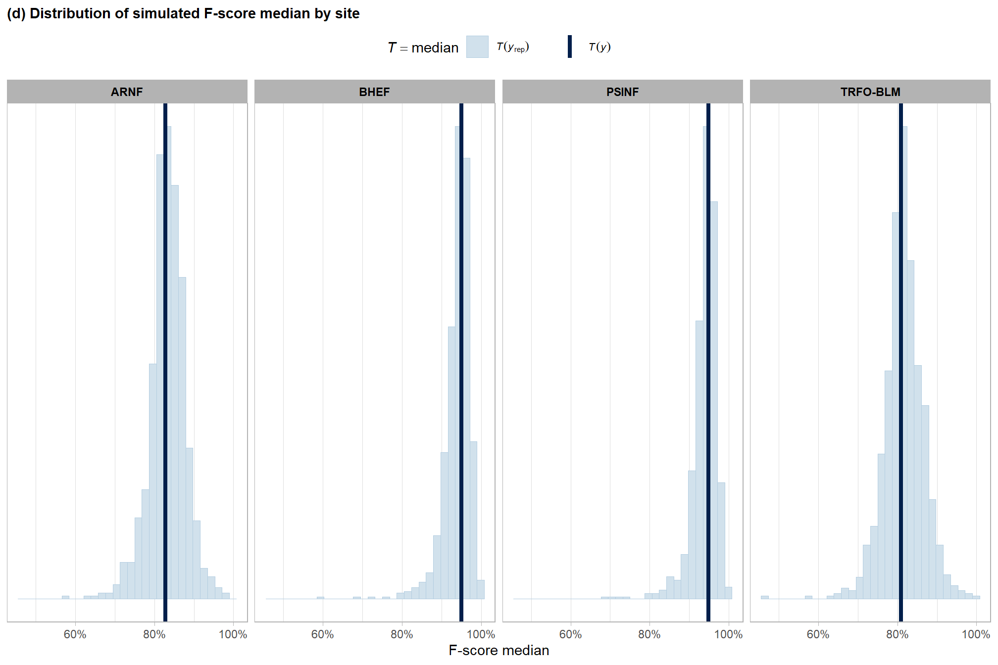

combine for manuscript

no_leg_temp <- 
  ggplot2::guides(
    color = "none", shape = "none"
    , fill = "none", size = "none"
  )
  # ggplot2::theme(legend.position = "none")
(
  p1_temp+ggplot2::theme(legend.position = "bottom")+
  p8_temp+no_leg_temp
) / 
  (p2_temp+no_leg_temp) / (p3_temp+no_leg_temp) +
  patchwork::plot_layout(guides = "collect") & 
  ggplot2::theme(
    legend.position = "bottom"
    , plot.subtitle = ggplot2::element_text(size = 10.5)
    , axis.text = ggplot2::element_text(size = 7.5)
    , axis.title.x = ggplot2::element_text(size = 7)
    , axis.title.y = ggplot2::element_text(size = 7)
    # , plot.tag = element_text(face = "bold", size = 11)
    # , plot.tag.position = c(0.17, 1.06)
    # , plot.margin = ggplot2::margin(t = 0.1, r = 0.1, b = 0.1, l = 0.1, unit = "in")
  )

# final_layout
ggplot2::ggsave("../data/bayes_ppc_chk1.jpeg", height = 10.5, width = 8.5, dpi = 300)

8.3.2.2 Model Results

quickly look at the model estimates of the effect of segmentation method

brms::fixef(fscore_mod_method_temp)

##             Estimate Est.Error       Q2.5     Q97.5
## Intercept  2.0394440 0.6747638  0.5293182 3.2932180
## method.L  -0.1524871 0.2039382 -0.5681992 0.2685544

# stats::coef(fscore_mod_method_temp)

plot the posterior predictive distributions of the conditional mean F-score by segmentation method with the 95% highest posterior density interval (HDI)

# get posterior draws
draws_temp <- agg_ground_truth_match_ans %>%
  dplyr::distinct(method) %>% 
  # re_formula = NA gives population average (average across site)
  tidybayes::add_epred_draws(fscore_mod_method_temp, re_formula = NA) %>% 
  dplyr::mutate(value = .epred) %>% 
  dplyr::ungroup()
# draws_temp %>% dplyr::count(method)
median_temp <- draws_temp %>% 
  dplyr::group_by(method) %>% 
  tidybayes::median_hdci(value)
# plot
plt_temp <- 
  draws_temp %>% 
  dplyr::mutate(method = forcats::fct_rev(method)) %>% 
  ggplot2::ggplot(
    mapping = aes(
      x = value
      , y = method
      , fill = method
    )
  ) +
  tidybayes::stat_halfeye(
    point_interval = tidybayes::median_hdci, .width = .95
    , interval_color = "gray66"
    , shape = 21, point_color = "gray66", point_fill = "black"
    , justification = -0.01
  ) +
  ggplot2::geom_text(
    data = median_temp
    , mapping = ggplot2::aes(x = value, label = scales::percent(value,accuracy = 0.1))
    , size = 3.5
    , hjust = 0.5, vjust = 2
  ) +
  ggplot2::geom_text(
    data = median_temp
    , mapping = ggplot2::aes(x = .upper, label = scales::percent(.upper,accuracy = 0.1))
    , size = 3
    , hjust = -0.1, vjust = 1
  ) +
  ggplot2::geom_text(
    data = median_temp
    , mapping = ggplot2::aes(x = .lower, label = scales::percent(.lower,accuracy = 0.1))
    , size = 3
    , hjust = 1.1, vjust = 1
  ) +
  # harrypotter::scale_fill_hp_d(option = "dracomalfoy", drop = F, direction = -1) +
  ggplot2::scale_fill_manual(values = c("plum2","plum4")) +
  ggplot2::scale_x_continuous(
    limits = c(0,1.05)
    , labels=scales::percent, breaks = scales::breaks_extended(n=6)
  ) +
  ggplot2::labs(
    subtitle = "posterior distribution of F-score by segmentation method\nand the 95% highest posterior density interval (HDI)"
    , x = "F-score", y = ""
  ) +
  ggplot2::theme_light() +
  ggplot2::theme(legend.position = "none", axis.text.y = ggplot2::element_text(face = "bold", size =11))
plt_temp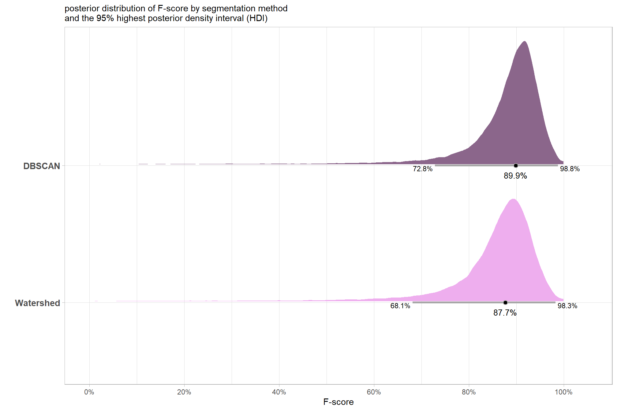

plt_temp <- plt_temp + ggplot2::theme(plot.title = ggplot2::element_blank(),plot.subtitle = ggplot2::element_blank())
ggplot2::ggsave("../data/bayes_method_pred.jpeg", plot = plt_temp, height = 7, width = 8.5, dpi = 300)

summary table of the posterior distribution and 95% HDI using tidybayes::median_hdci() to avoid potential for returning multiple rows by group if our data is grouped. See the documentation for the ggdist package which notes that “If the distribution is multimodal, hdi may return multiple intervals for each probability level (these will be spread over rows).”

median_temp %>% 
  dplyr::select(-c(.point,.interval, .width)) %>% 
  dplyr::mutate(
    dplyr::across(
      dplyr::where(is.numeric)
      , ~scales::percent(.x,accuracy=0.1)
    )
  ) %>% 
  kableExtra::kbl(
    digits = 2
    , caption = "F-score<br>95% HDI of the posterior predictive distribution"
    , col.names = c(
      "method"
      , "F-score<br>median"
      , "HDI low", "HDI high"
    )
    , escape = F
  ) %>% 
  kableExtra::kable_styling()

Table 8.3: F-score
95% HDI of the posterior predictive distribution
method	F-score median	HDI low	HDI high
DBSCAN	89.9%	72.8%	98.8%
Watershed	87.7%	68.1%	98.3%

we can also make pairwise comparisons using the posterior draws with tidybayes::compare_levels() to determine the difference in F-score between the two methods, but now, instead of one mean difference value as in the paired t-test, we get a distribution of the difference which provides much more detailed insight to the difference in detection accuracy between the two segmentation methods

comp_temp <- draws_temp %>%
  tidybayes::compare_levels(
    value
    , by = method
    # make the comparison the same as t.test: dbscan-watershed
    , comparison = list(c("DBSCAN","Watershed"))
  )
# dplyr::glimpse(comp_temp)
med_comp_temp <- tidybayes::median_hdci(comp_temp$value)
mean_comp_temp <- tidybayes::mean_hdci(comp_temp$value)
# plot
plt_temp <-
  comp_temp %>% 
  ggplot2::ggplot(mapping=ggplot2::aes( y = 0)) +
  ggplot2::geom_vline(
    xintercept = 0
    # , linetype = "dashed"
    , color = "gray77"
    , lwd = 1.2
  ) +
  tidybayes::stat_halfeye(
    mapping = ggplot2::aes(x = value)
    , point_interval = tidybayes::median_hdci, .width = .95
    , fill = "thistle4", alpha = 0.9
    , interval_color = "gray66"
    , shape = 21, point_color = "gray66", point_fill = "black"
    , justification = -0.01
  ) +
  # ggplot2::annotate(
  #   "text"
  #   , x = (med_comp_temp %>% dplyr::select(y,ymin,ymax) %>% base::unlist(use.names = F))
  #   , y = -0.01
  #   , label = (
  #     med_comp_temp %>% 
  #       dplyr::select(y,ymin,ymax) %>% 
  #       base::unlist(use.names = F) %>% 
  #       scales::percent(accuracy = 0.1)
  #   )
  # ) +
  ggplot2::geom_text(
    data = med_comp_temp
    , mapping = ggplot2::aes(x = y, label = scales::percent(y,accuracy = 0.1))
    , size = 3.5
    , hjust = 0.5, vjust = 2
  ) +
  ggplot2::geom_text(
    data = med_comp_temp
    , mapping = ggplot2::aes(x = ymax, label = scales::percent(ymax,accuracy = 0.1))
    , size = 3
    , hjust = -0.1, vjust = 1
  ) +
  ggplot2::geom_text(
    data = med_comp_temp
    , mapping = ggplot2::aes(x = ymin, label = scales::percent(ymin,accuracy = 0.1))
    , size = 3
    , hjust = 1.1, vjust = 1
  ) +
  ggplot2::scale_y_continuous(breaks=NULL) +
  ggplot2::scale_x_continuous(labels=scales::percent, breaks = scales::breaks_extended(n=8), expand = ggplot2::expansion(mult = 0.05)) +
  ggplot2::labs(
    subtitle = "difference in F-score between segmentation methods"
    , x = "difference in F-score\n(DBSCAN - Watershed)"
    , y = "" # "difference: DBSCAN - Watershed"
  ) +
  ggplot2::theme_light() +
  ggplot2::theme(
    # axis.title.y = ggplot2::element_text(angle = 0, vjust = 0.5)
    # , axis.text.y = ggplot2::element_text(face = "bold", size =11)
    axis.title.x = ggplot2::element_text(face = "bold", size =11)
    , axis.title.y = ggplot2::element_blank()
  )
plt_temp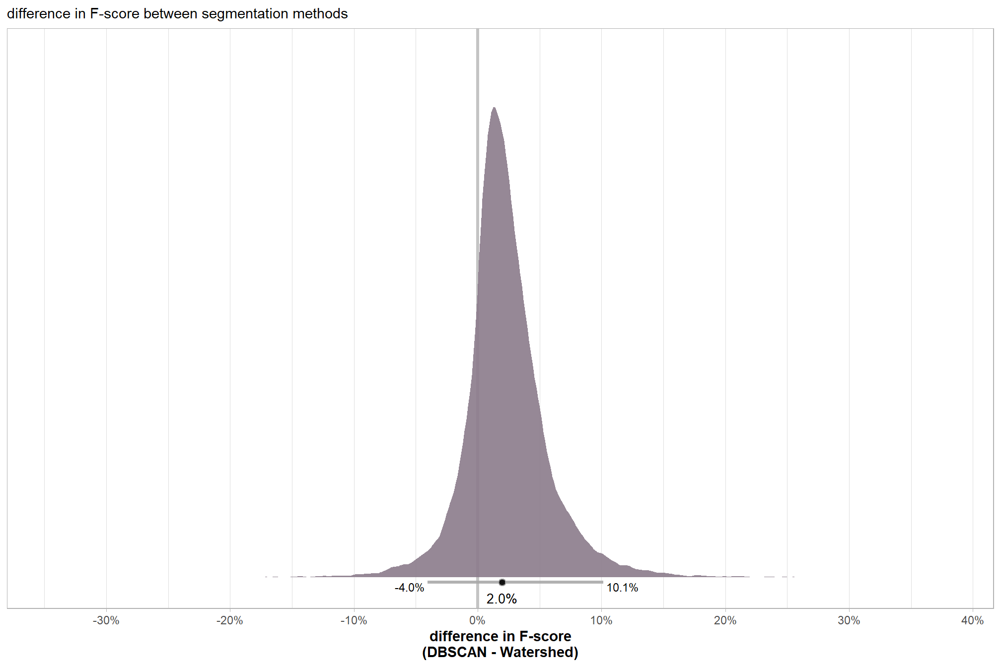

plt_temp <- plt_temp + ggplot2::theme(plot.title = ggplot2::element_blank(),plot.subtitle = ggplot2::element_blank())
ggplot2::ggsave("../data/bayes_method_diff_pred.jpeg", plot = plt_temp, height = 7, width = 8.5, dpi = 300)
# scales::percent(mean_comp_temp$y,accuracy=0.1)
# scales::percent(ttest_temp$estimate, accuracy = 0.1)

the 95% HDI shown as the gray line below the posterior distribution summarizes the posterior draws to represent a density interval with a value of central tendency. We plot the median (2.0%) as the value of central tendency of the difference in F-score between the two methods but we could also determine the mean difference which we calculated above using tidybayes::mean_hdci(). Our Bayesian approach estimates the mean difference in F-score between the two methods as 2.3% which we can directly compare to the mean difference tested using the paired t-test above of 2.2%.

table the 95% HDI of the difference in F-score between the two methods

med_comp_temp %>% 
  dplyr::mutate(
    dplyr::across(
      dplyr::where(is.numeric)
      , ~scales::percent(.x,accuracy=0.1)
    )
  ) %>% 
  dplyr::select(tidyselect::starts_with("y")) %>% 
  dplyr::mutate(d = "difference (DBSCAN - Watershed)") %>% 
  dplyr::relocate(d) %>% 
  kableExtra::kbl(
    caption = "difference in F-score between the two methods<br>95% HDI of the posterior predictive distribution"
    , col.names = c(
      ""
      , "difference F-score<br>median"
      , "HDI low", "HDI high"
    )
    , escape = F
  ) %>% 
  kableExtra::kable_styling()

Table 8.4: difference in F-score between the two methods
95% HDI of the posterior predictive distribution
	difference F-score median	HDI low	HDI high
difference (DBSCAN - Watershed)	2.0%	-4.0%	10.1%

finally, we can use the posterior draws of the difference in F-score (calculated with tidybayes::compare_levels()) to determine the probability that one method is better than the other

comp_temp <- comp_temp %>% 
  dplyr::mutate(
    diff_gt_0 = as.numeric(value>0)
  ) 
# simply calculate the proportion of posterior draws where the difference is greater than zero
mean(comp_temp$diff_gt_0) %>% scales::percent(accuracy = 0.1)

## [1] "81.9%"

There is a 81.9% probability that the DBSCAN method results in better slash pile detection accuracy (i.e. higher F-score) than the Watershed method

8.4 Individual Pile Evaluation

let’s visually inspect the TP, FP, and FN predictions to see if we can get some insight into why actual piles were missed (omissions) or correctly predicted (TP) and why the method may have made incorrect predictions (commissions)

p_fn_temp <- function(row_n = 1, site, method = "dbscan", mtchgrp = "true positive") {
  if(tolower(method) == "dbscan"){
    w_dta <- dbscan_gt_pred_match[[site]] %>% 
      dplyr::filter(match_grp == mtchgrp)
    p_dta <- dbscan_spectral_preds[[site]]
  }else{
    w_dta <- watershed_gt_pred_match[[site]] %>% 
      dplyr::filter(match_grp == mtchgrp)
    p_dta <- watershed_spectral_preds[[site]]
  }
  # get area of largest with buffer so all plots are same size
  if(site %in% c("bhef")){
    b <- 8.5
  }else if(site %in% c("arnf")){
    b <- 6
  }else{
    b <- 4
  }
  
  if(
    mtchgrp %in%  c("true positive", "omission")
  ){
    area_temp <- slash_piles_polys[[site]] %>% 
      dplyr::inner_join(
        w_dta %>% 
          dplyr::slice_max(order_by = gt_area_m2, n = 1) 
        , by = "pile_id"
      ) %>% 
      sf::st_transform(crs=terra::crs(rgb_rast[[site]])) %>% 
      sf::st_buffer(b) %>% 
      sf::st_area() %>% 
      as.numeric() %>% 
      ceiling() 
  }else{
    area_temp <- p_dta %>% 
      dplyr::inner_join(
        w_dta %>% 
          dplyr::slice_max(order_by = pred_area_m2, n = 1) 
        , by = "pred_id"
      ) %>% 
      sf::st_transform(crs=terra::crs(rgb_rast[[site]])) %>% 
      sf::st_buffer(b) %>% 
      sf::st_area() %>% 
      as.numeric() %>% 
      ceiling()
  }
  # tp
  tp <- w_dta %>% dplyr::slice(row_n)
  # ortho area
  if(mtchgrp %in%  c("true positive")){
    # gt pile
    gt_pile <- slash_piles_polys[[site]] %>% 
      dplyr::filter(pile_id == tp$pile_id)
    # pred pile
    pred_pile <- p_dta %>% 
      dplyr::filter(pred_id == tp$pred_id)
    
    ortho_st <- 
      sf::st_union(
        gt_pile %>% sf::st_transform(crs=terra::crs(rgb_rast[[site]])) 
        , pred_pile %>% sf::st_transform(crs=terra::crs(rgb_rast[[site]])) 
      ) %>% 
      sf::st_centroid() %>% 
      sf::st_buffer(
        sqrt(area_temp/4) ## numerator = desired plot size in m2
        , endCapStyle = "SQUARE"
      ) %>%
      dplyr::mutate(dummy=1)  
  }else if(
    mtchgrp %in%  c("omission")
  ){
    # gt pile
    gt_pile <- slash_piles_polys[[site]] %>% 
      dplyr::filter(pile_id == tp$pile_id)
    ortho_st <- 
      gt_pile %>% 
      sf::st_transform(crs=terra::crs(rgb_rast[[site]])) %>% 
      sf::st_centroid() %>% 
      sf::st_buffer(
        sqrt(area_temp/4) ## numerator = desired plot size in m2
        , endCapStyle = "SQUARE"
      ) %>%
      dplyr::mutate(dummy=1)  
  }else if(
    mtchgrp %in%  c("commission")
  ){
    # pred pile
    pred_pile <- p_dta %>% 
      dplyr::filter(pred_id == tp$pred_id)
    ortho_st <- 
      pred_pile %>% 
      sf::st_transform(crs=terra::crs(rgb_rast[[site]])) %>% 
      sf::st_centroid() %>% 
      sf::st_buffer(
        sqrt(area_temp/4) ## numerator = desired plot size in m2
        , endCapStyle = "SQUARE"
      ) %>%
      dplyr::mutate(dummy=1)  
  }
  
  # get plt
  rp <- ortho_plt_fn(
    rgb_rast = rgb_rast[[site]]
    , stand = ortho_st
    , add_stand = F
    , buffer = 0
  ) 
  
  # #### add chm?
  # if(addchm){
  #   # get max ht
  #   maxh <- all_stand_boundary %>% 
  #     dplyr::filter(site_data_lab == site) %>% 
  #     dplyr::slice(1) %>% 
  #     dplyr::pull(max_ht_m)
  #   # ff <- tempfile(fileext = ".tif")
  #   # crop, slice rast
  #   ##### ???????????????????????? this kills your computer every time :\
  #   crp_chm_rast_temp <- chm_rast[[site]] %>% 
  #     terra::crop(
  #       ortho_st %>% 
  #         dplyr::ungroup() %>% 
  #         sf::st_union() %>% 
  #         sf::st_bbox() %>% 
  #         sf::st_as_sfc() %>% 
  #         sf::st_transform(terra::crs(chm_rast[[site]])) %>% 
  #         terra::vect()
  #       , mask = T
  #       # , filename = ff
  #     )
  #   crp_chm_rast_temp <- 
  #     # slice
  #     terra::clamp(
  #       crp_chm_rast_temp
  #       , upper = maxh
  #       , lower = 0
  #       , values = F
  #     )
  #   rp <- rp +
  #     ggnewscale::new_scale_fill() +
  #     ggplot2::geom_tile(
  #       data = crp_chm_rast_temp %>%
  #         terra::as.data.frame(xy=T) %>%
  #         dplyr::rename(f=3)
  #       , mapping = ggplot2::aes(x=x,y=y,fill=f)
  #       , alpha = 0.5
  #       , inherit.aes = F
  #     ) +
  #     ggplot2::scale_fill_viridis_c(
  #       option = "plasma", na.value = "gray",name = "CHM (m)"
  #       , limits = c(0,ceiling(maxh))
  #     )
  # }
  
  #### add piles
  if(mtchgrp %in%  c("true positive", "omission")){
    rp <- rp +
      ggplot2::geom_sf(data = gt_pile, fill = NA, color = "cyan", lwd = 0.6)
  }
  if(mtchgrp %in%  c("true positive", "commission")){
    rp <- rp +
      ggplot2::geom_sf(data = pred_pile, fill = NA, color = "magenta", lwd = 0.5)
  }
  
  
  
  return(
    rp
    # list(rp,ortho_st)
  )
}

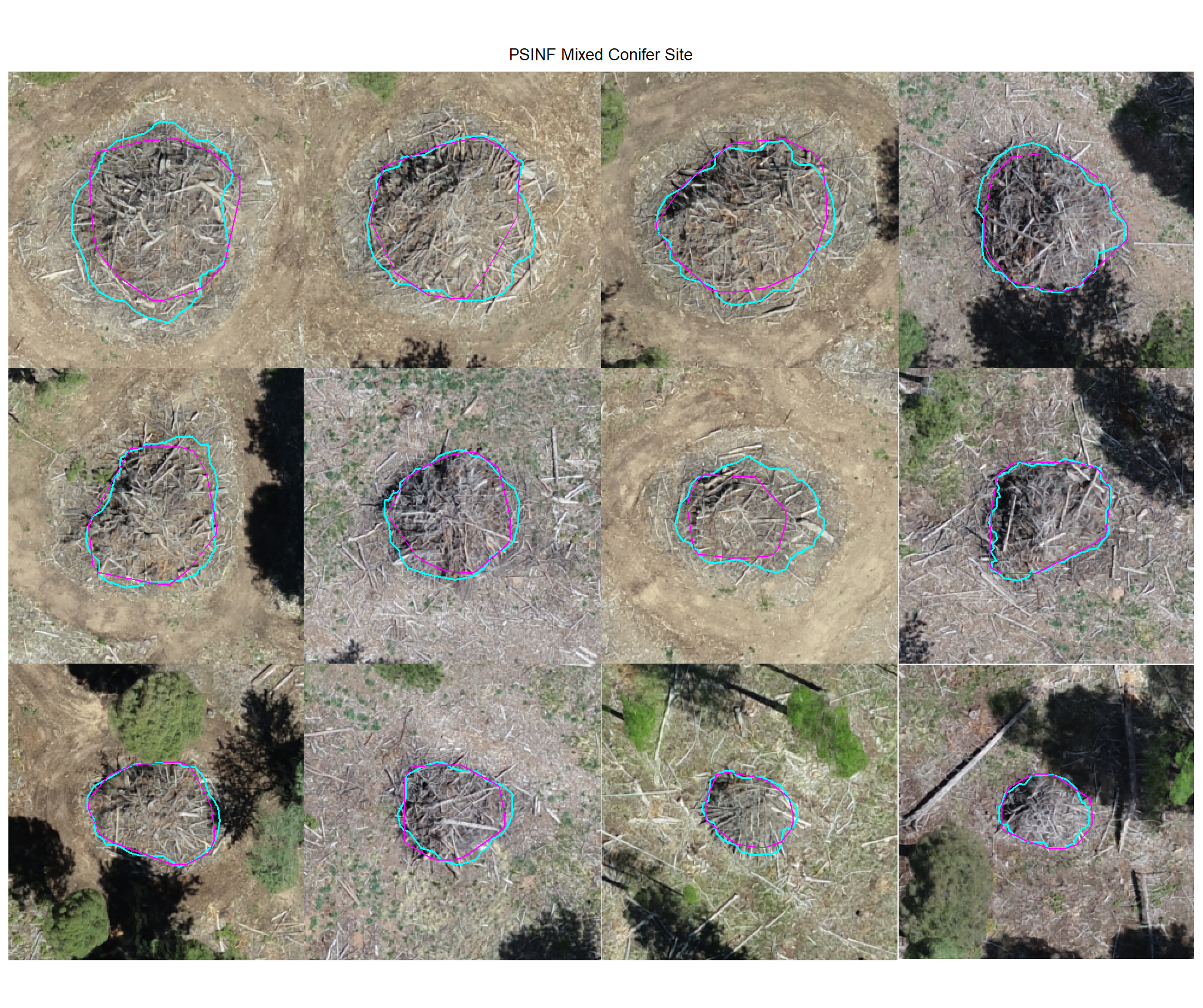
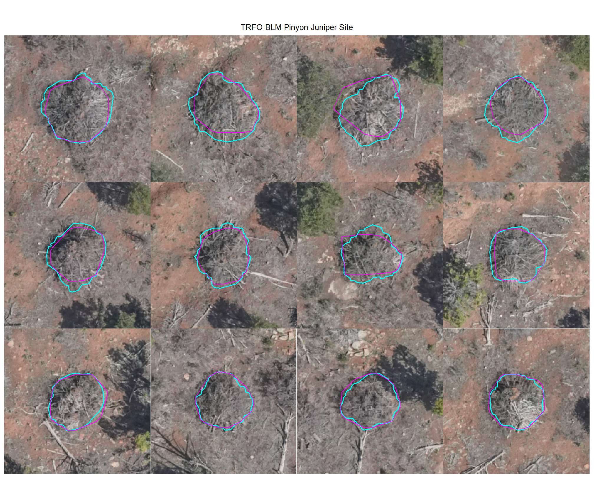
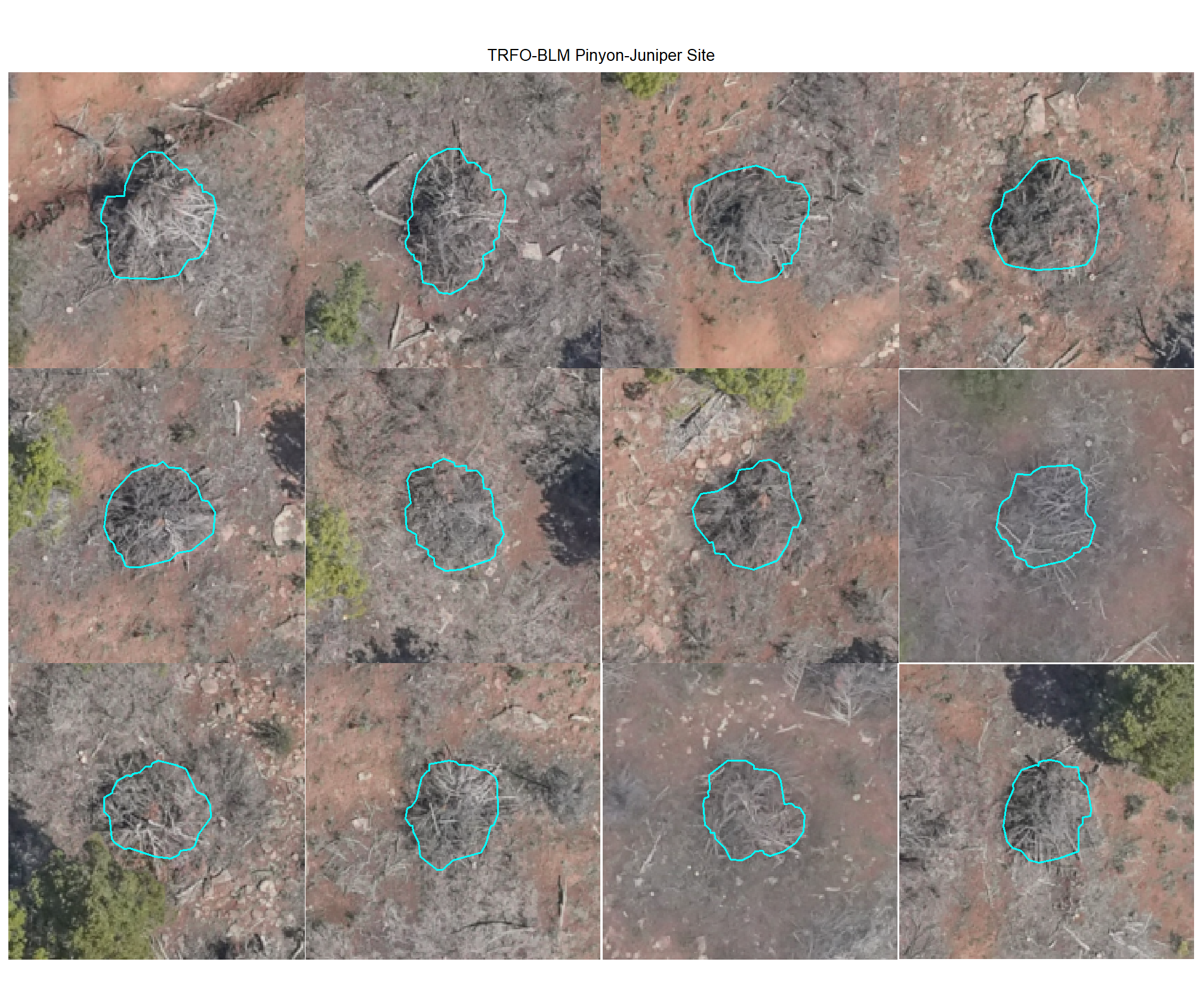
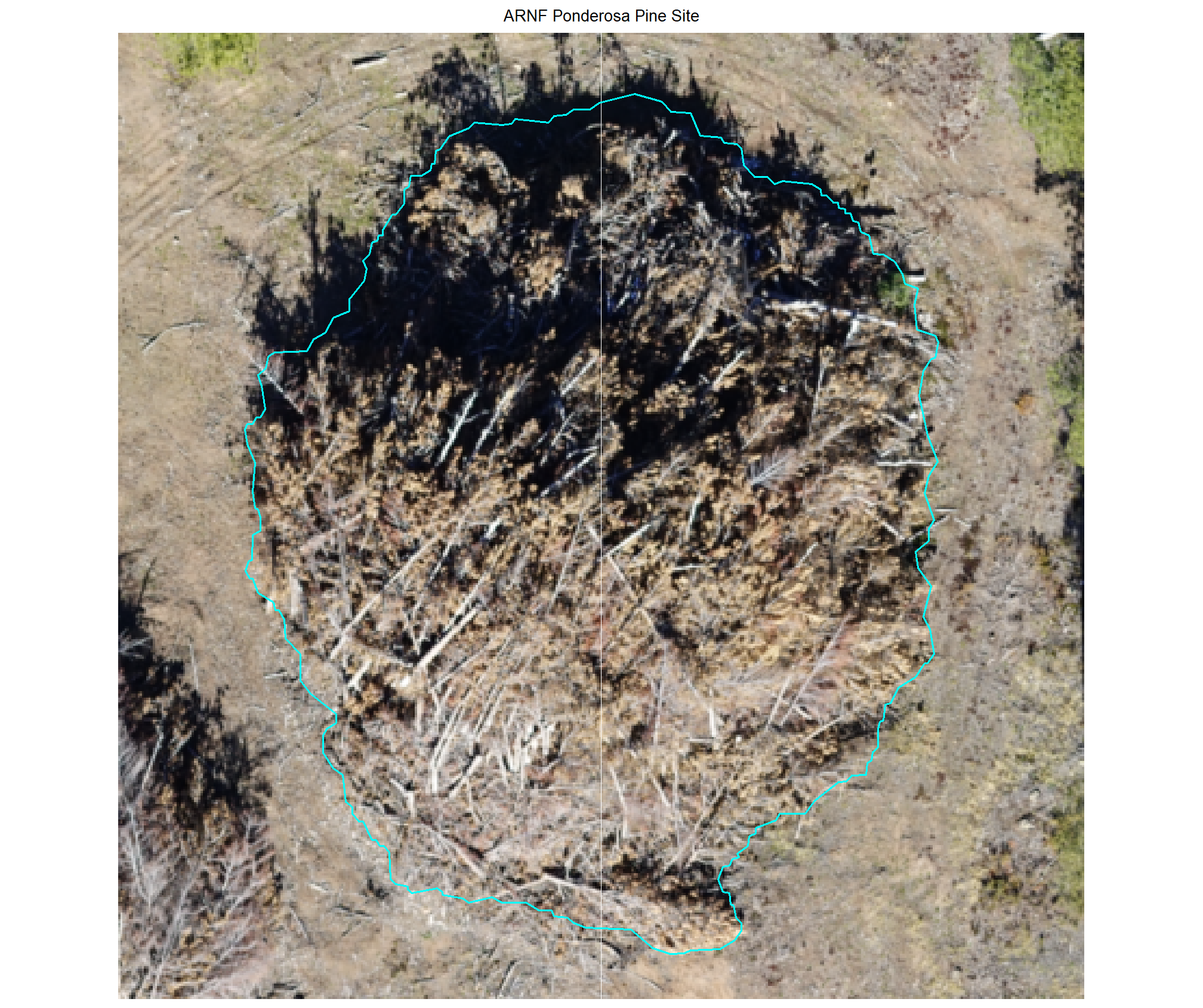
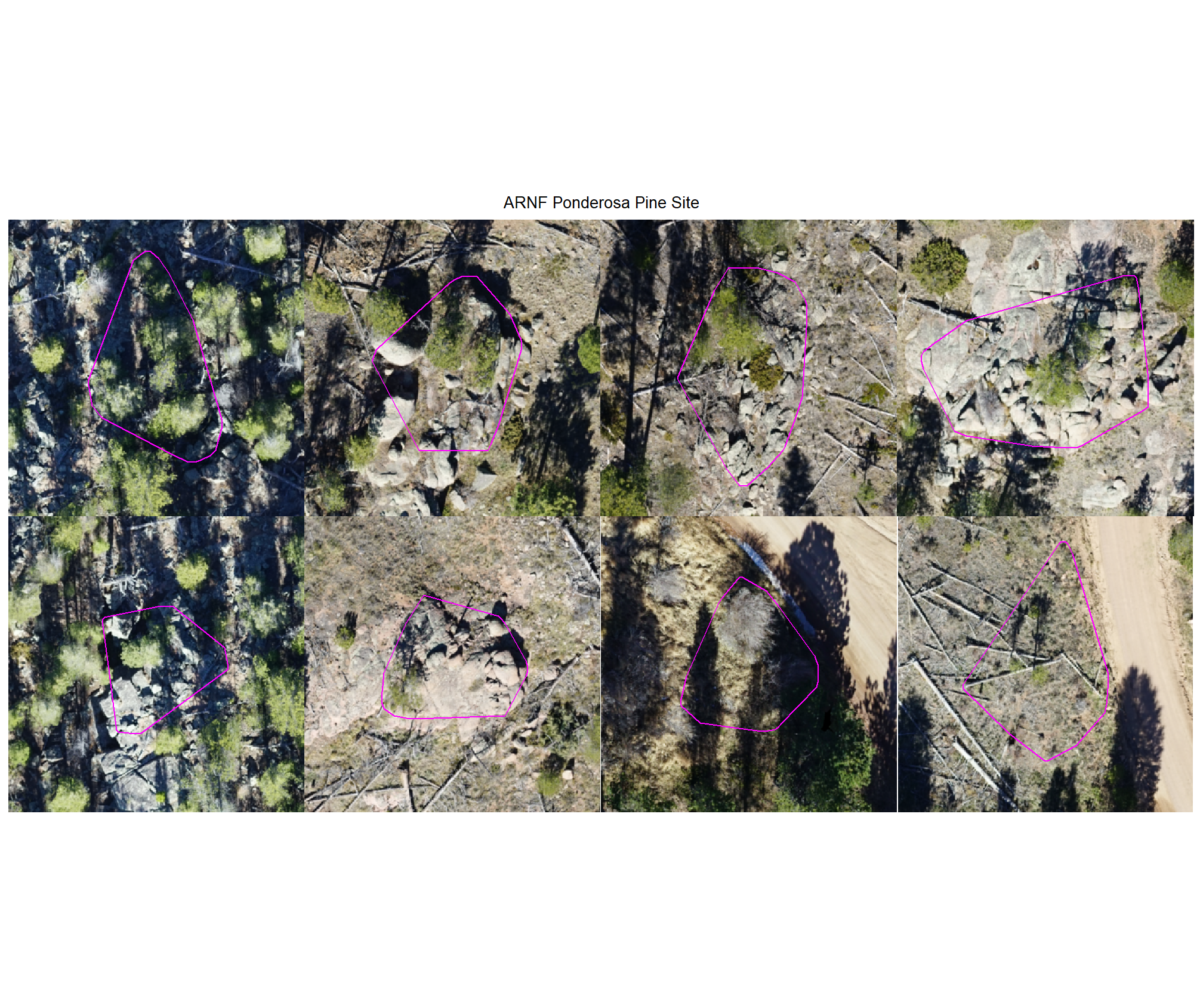
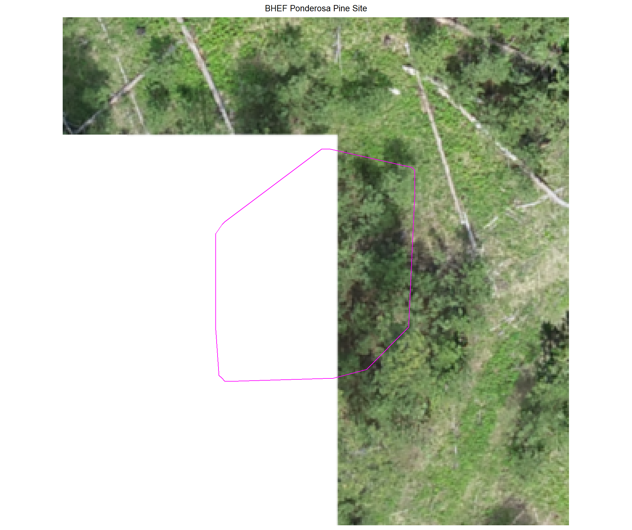
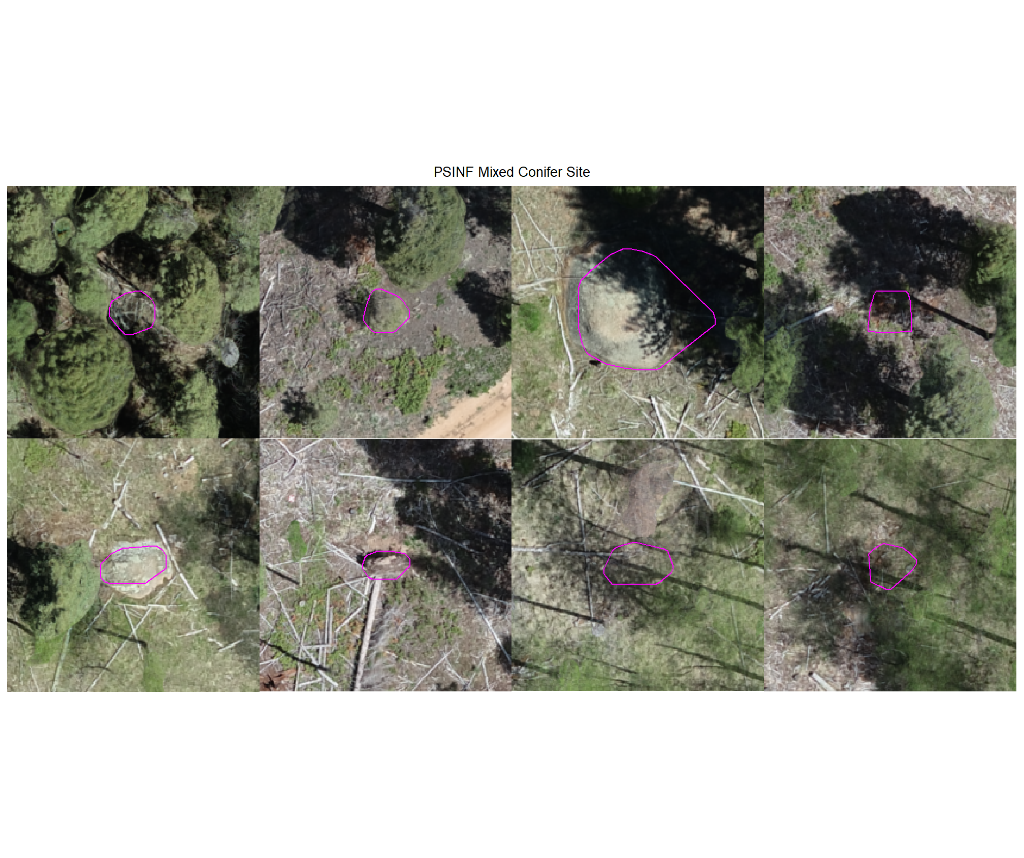
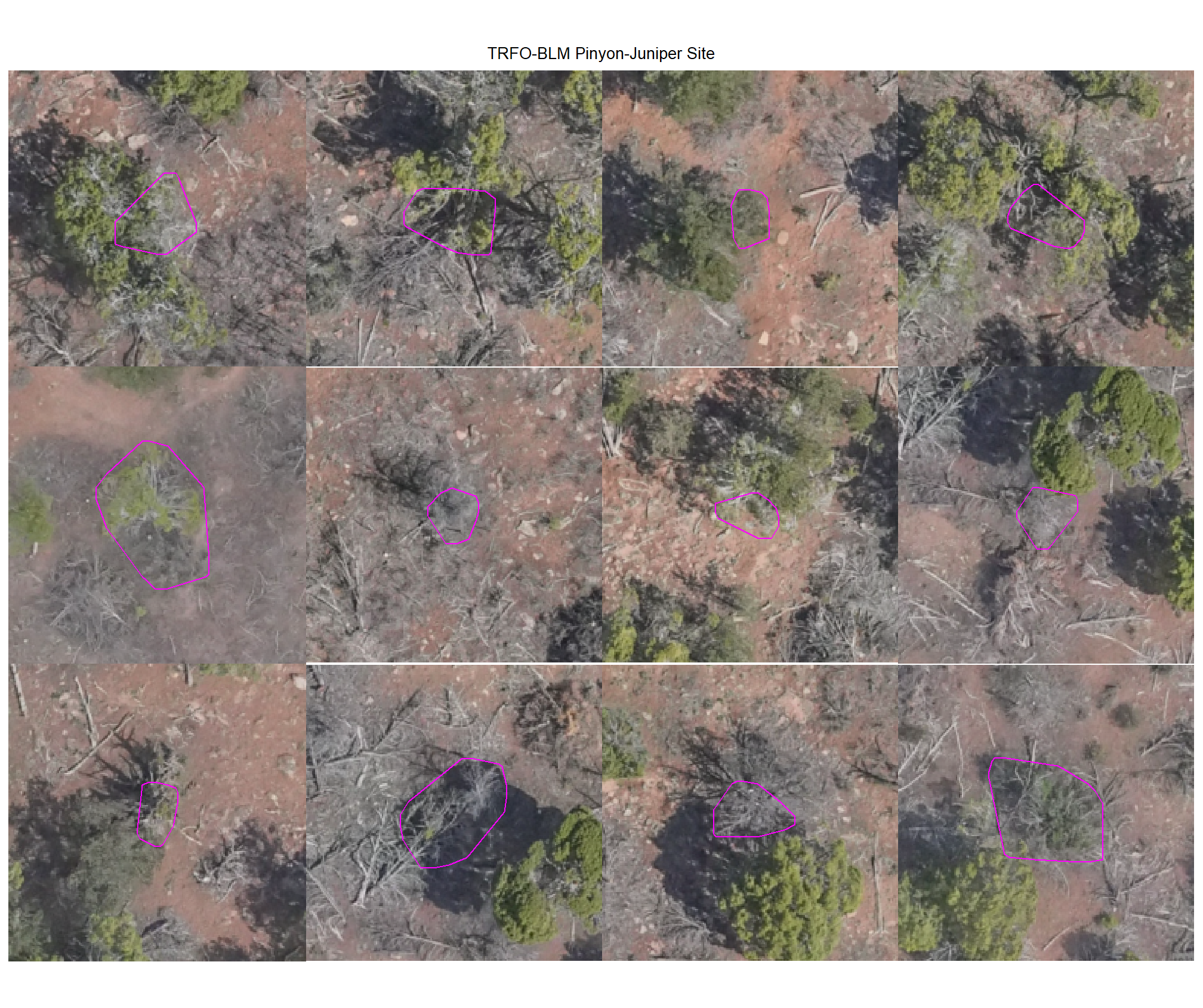
8.4.1 True Positives

Check out the plots for the TP matches

# max piles per site
nplts_temp <- 12
# dbscan
dbscan_tp_plts_temp <- all_stand_boundary$site_data_lab %>% 
  purrr::set_names() %>% 
  purrr::map(
    function(x){
      nn <- 
        dbscan_gt_pred_match[[x]] %>% 
        dplyr::filter(match_grp == "true positive") %>% 
        nrow()
      if(nn==0){return(NULL)}
      pl <- 
        1:min(nn,nplts_temp) %>% 
        purrr::map(
          \(r)
          p_fn_temp(row_n = r, site = x, method = "dbscan", mtchgrp = "true positive")
        )
      return(pl)
    }
  )
# watershed
watershed_tp_plts_temp <- all_stand_boundary$site_data_lab %>% 
  purrr::set_names() %>% 
  purrr::map(
    function(x){
      nn <- 
        watershed_gt_pred_match[[x]] %>% 
        dplyr::filter(match_grp == "true positive") %>% 
        nrow()
      if(nn==0){return(NULL)}
      pl <- 
        1:min(nn,nplts_temp) %>% 
        purrr::map(
          \(r)
          p_fn_temp(row_n = r, site = x, method = "watershed", mtchgrp = "true positive")  
        )
      return(pl)
    }
  )

8.4.1.1 DBSCAN

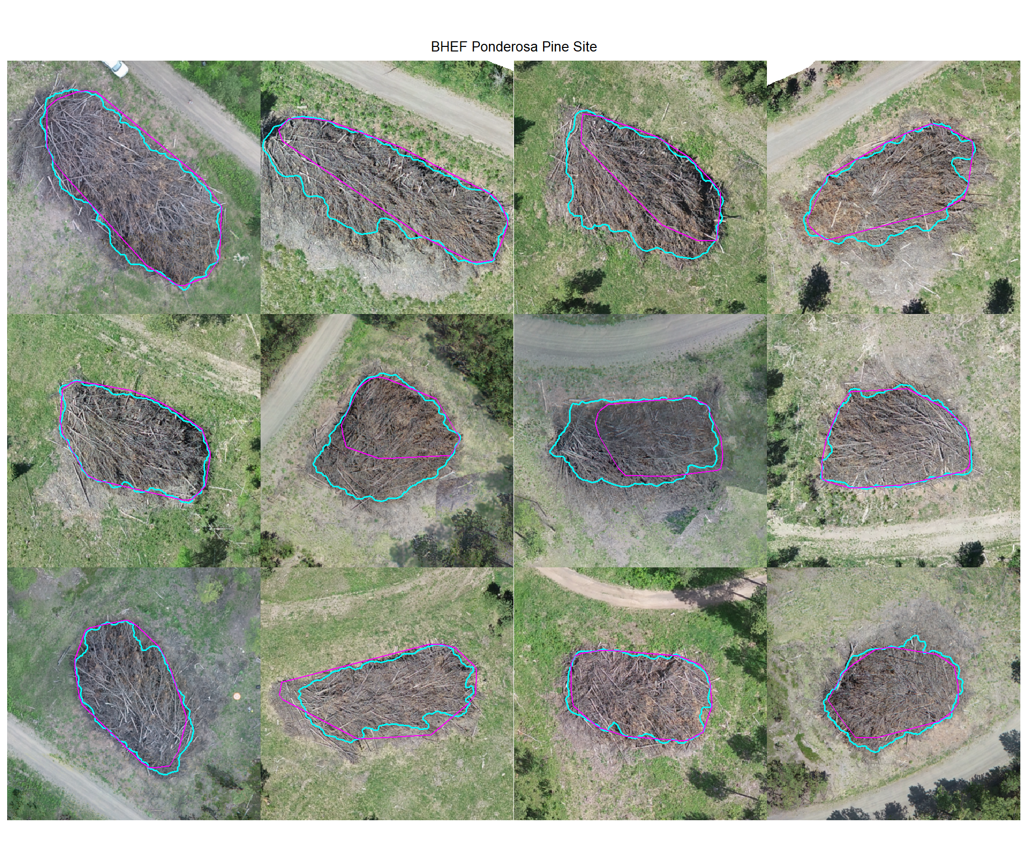
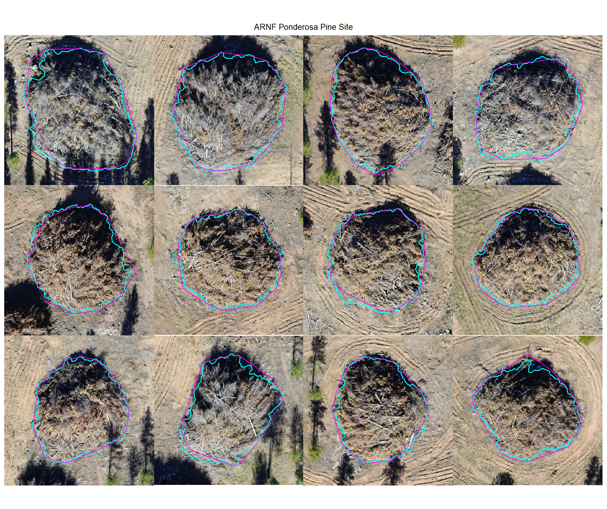
plot example true positive matches on the RGB with the actual pile (cyan) and predicted (magenta) pile outlined

all_stand_boundary$site_data_lab %>% 
purrr::map(
  function(x){
  if(any(is.null(dbscan_tp_plts_temp[[x]]))){return(NULL)}
  l <- dbscan_tp_plts_temp[[x]] %>% length()
  dbscan_tp_plts_temp[[x]] %>% 
  # purrr::map(1) %>% 
  # purrr::keep_at(1:4) %>% 
  patchwork::wrap_plots(ncol = min(l,4)) +
  patchwork::plot_annotation(
    title = all_stand_boundary %>% dplyr::filter(site_data_lab==x) %>% dplyr::pull(site)
    , theme = ggplot2::theme(plot.title = ggplot2::element_text(size = 10, hjust = 0.5))
  )
})

8.4.1.2 Watershed

plot example true positive matches on the RGB with the actual pile (cyan) and predicted (magenta) pile outlined

all_stand_boundary$site_data_lab %>% 
purrr::map(
  function(x){
  if(any(is.null(watershed_tp_plts_temp[[x]]))){return(NULL)}
  l <- watershed_tp_plts_temp[[x]] %>% length()
  watershed_tp_plts_temp[[x]] %>% 
  # purrr::map(1) %>% 
  # purrr::keep_at(1:4) %>% 
  patchwork::wrap_plots(ncol = min(l,4)) +
  patchwork::plot_annotation(
    title = all_stand_boundary %>% dplyr::filter(site_data_lab==x) %>% dplyr::pull(site)
    , theme = ggplot2::theme(plot.title = ggplot2::element_text(size = 10, hjust = 0.5))
  )
})

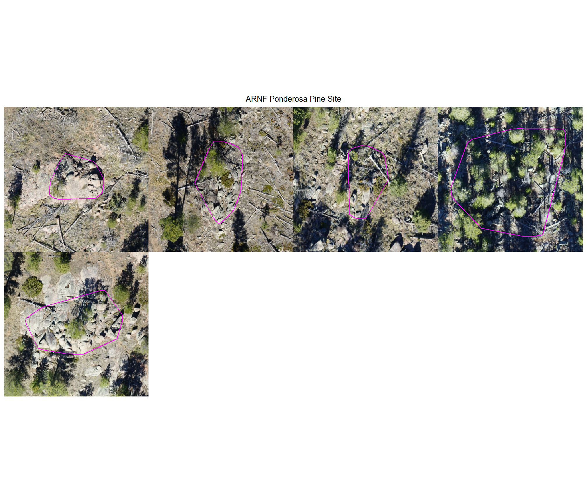
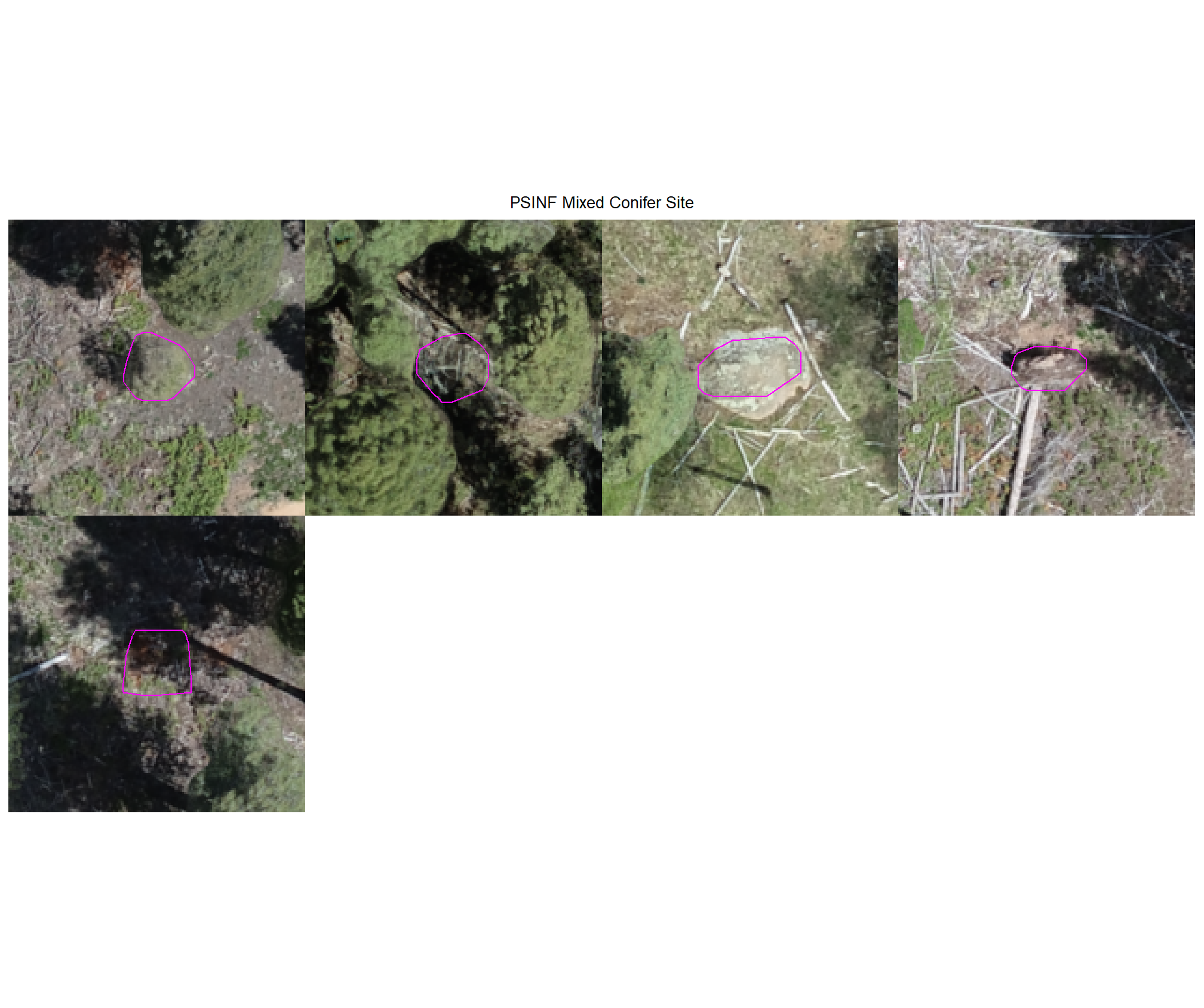
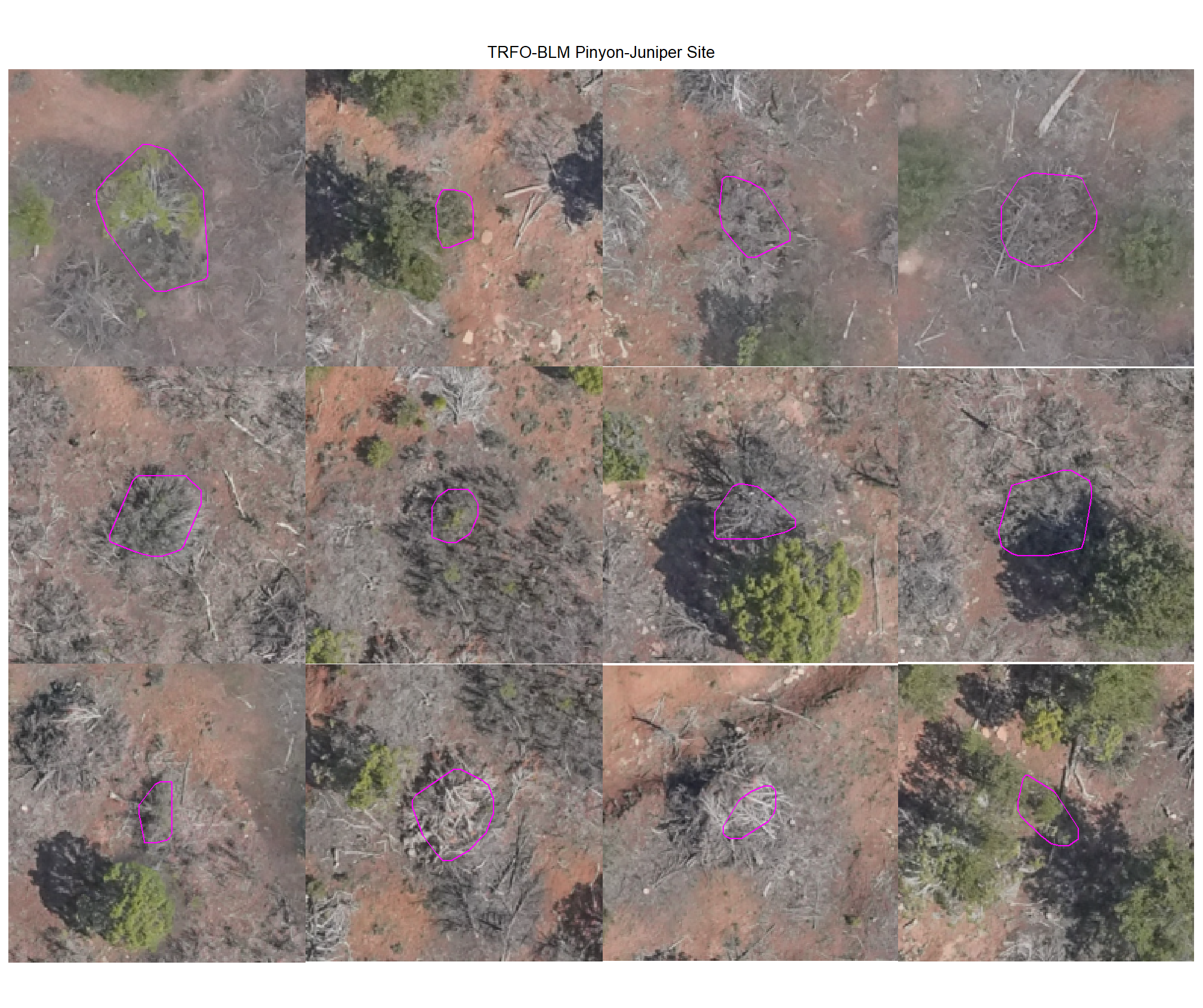
8.4.2 Omissions (False Negatives)

Check out the plots for the omissions (FN)

# dbscan
dbscan_tp_plts_temp <- all_stand_boundary$site_data_lab %>% 
  purrr::set_names() %>% 
  purrr::map(
    function(x){
      nn <- 
        dbscan_gt_pred_match[[x]] %>% 
        dplyr::filter(match_grp == "omission") %>% 
        nrow()
      if(nn==0){return(NULL)}
      pl <- 
        1:min(nn,nplts_temp) %>% 
        purrr::map(
          \(r)
          p_fn_temp(row_n = r, site = x, method = "dbscan", mtchgrp = "omission")  
        )
      return(pl)
    }
  )
# watershed
watershed_tp_plts_temp <- all_stand_boundary$site_data_lab %>% 
  purrr::set_names() %>% 
  purrr::map(
    function(x){
      nn <- 
        watershed_gt_pred_match[[x]] %>% 
        dplyr::filter(match_grp == "omission") %>% 
        nrow()
      if(nn==0){return(NULL)}
      pl <- 
        1:min(nn,nplts_temp) %>% 
        purrr::map(
          \(r)
          p_fn_temp(row_n = r, site = x, method = "watershed", mtchgrp = "omission")  
        )
      return(pl)
    }
  )

8.4.2.1 DBSCAN

plot example omissions on the RGB with the actual pile (cyan) pile outlined

all_stand_boundary$site_data_lab %>% 
purrr::map(
  function(x){
  if(any(is.null(dbscan_tp_plts_temp[[x]]))){return(NULL)}
  l <- dbscan_tp_plts_temp[[x]] %>% length()
  dbscan_tp_plts_temp[[x]] %>% 
  # purrr::map(1) %>% 
  # purrr::keep_at(1:4) %>% 
  patchwork::wrap_plots(ncol = min(l,4)) +
  patchwork::plot_annotation(
    title = all_stand_boundary %>% dplyr::filter(site_data_lab==x) %>% dplyr::pull(site)
    , theme = ggplot2::theme(plot.title = ggplot2::element_text(size = 10, hjust = 0.5))
  )
})

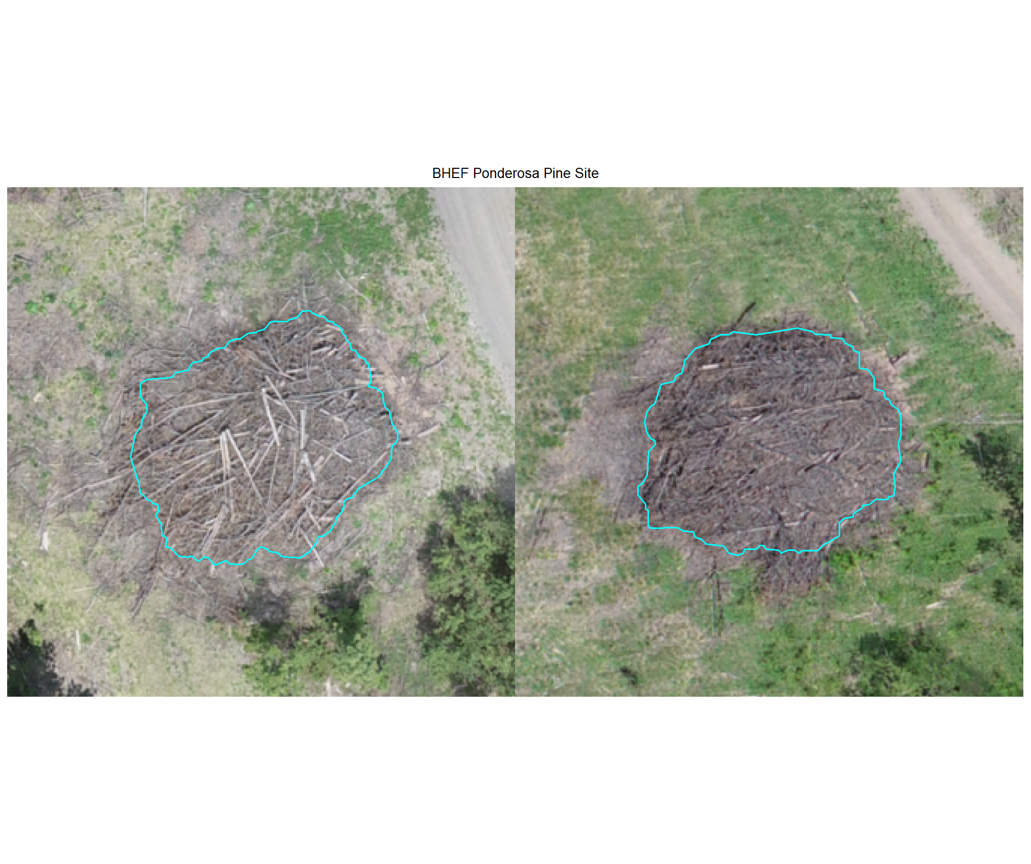
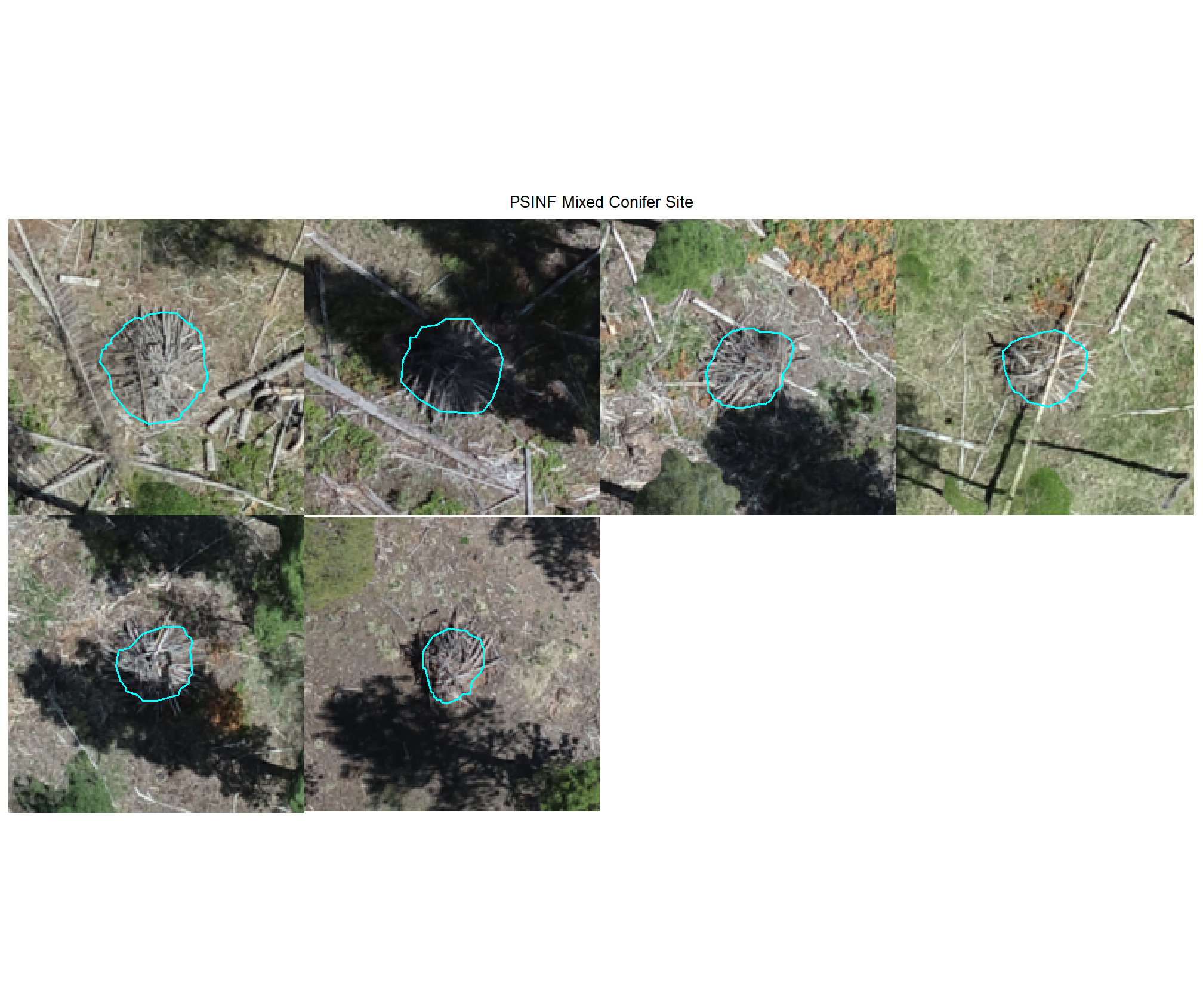
8.4.2.2 Watershed

plot example omissions on the RGB with the actual pile (cyan) pile outlined

all_stand_boundary$site_data_lab %>% 
purrr::map(
  function(x){
  if(any(is.null(watershed_tp_plts_temp[[x]]))){return(NULL)}
  l <- watershed_tp_plts_temp[[x]] %>% length()
  watershed_tp_plts_temp[[x]] %>% 
  # purrr::map(1) %>% 
  # purrr::keep_at(1:4) %>% 
  patchwork::wrap_plots(ncol = min(l,4)) +
  patchwork::plot_annotation(
    title = all_stand_boundary %>% dplyr::filter(site_data_lab==x) %>% dplyr::pull(site)
    , theme = ggplot2::theme(plot.title = ggplot2::element_text(size = 10, hjust = 0.5))
  )
})

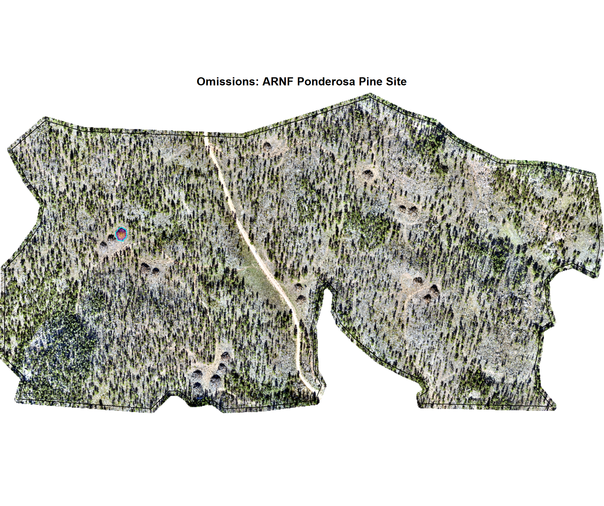
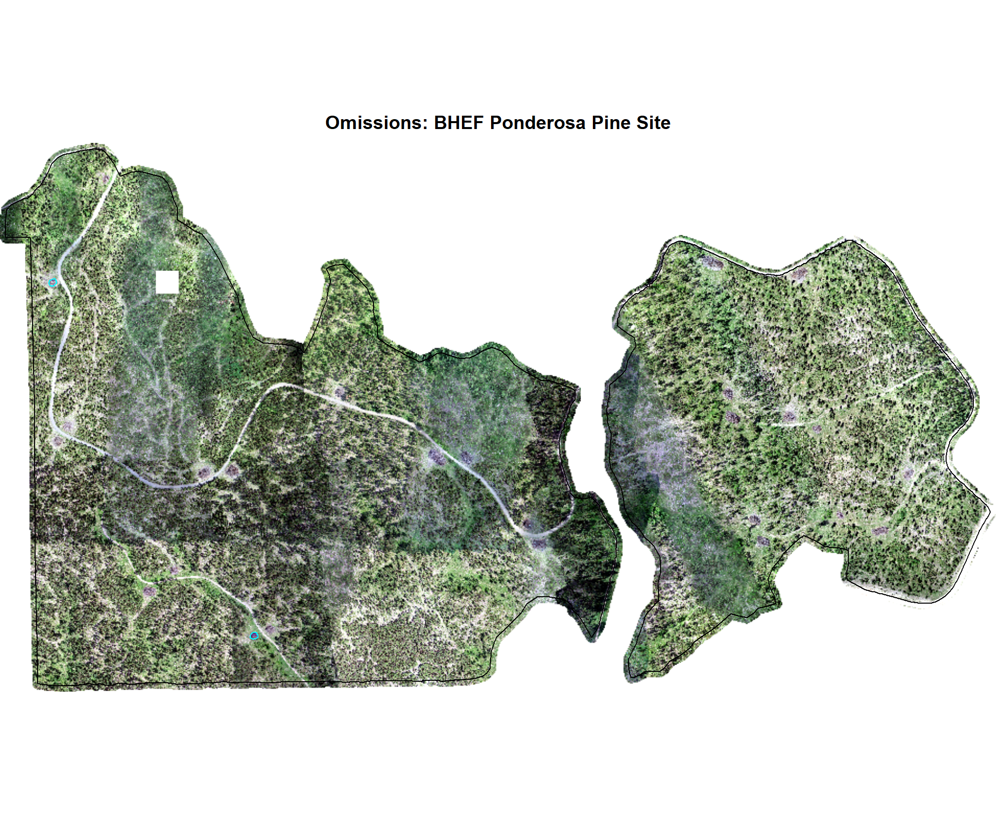
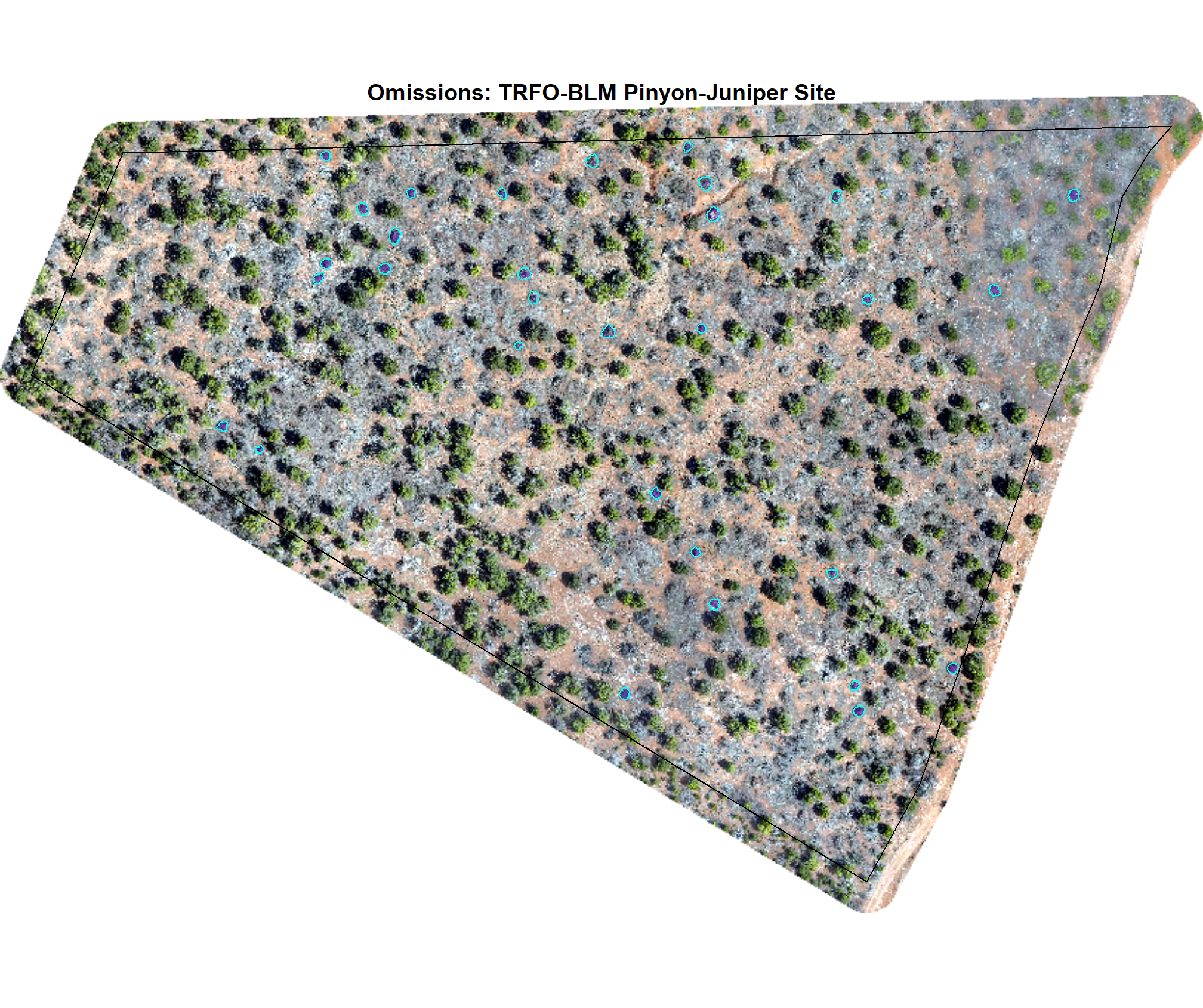
8.4.2.3 Omissions with CHM and RGB

why are these missing?

# function to plot ortho
terra_plt_ortho <- function(
  ortho
  , gt_piles = NA
  , pred_piles = NA
  , boundary
  , title
  , chm = NA
  , maxh = 99
) {
  terra::plotRGB(ortho, stretch = "lin")
  terra::plot(
    boundary %>% 
      sf::st_transform(terra::crs(ortho)) %>% 
      terra::vect()
    , add = T, border = "black", col = NA
    , main = title
  )
  if(inherits(chm,"SpatRaster")){
    terra::plot(
      chm
      , add = T, col = viridis::plasma(n=100), alpha = 0.5
      , legend = F
      , range = c(0,maxh), fill_range = T
    )
  }
  if(!all(is.na(gt_piles))){
    terra::plot(
      gt_piles %>% 
        dplyr::filter(is_in_stand) %>% 
        sf::st_transform(terra::crs(ortho)) %>% 
        terra::vect()
      , add = T, border = "cyan", col = NA, lwd = 1.2
    )
  }
  if(!all(is.na(pred_piles))){
    terra::plot(
      pred_piles %>% 
        sf::st_transform(terra::crs(ortho)) %>% 
        terra::vect()
      , add = T, border = "magenta", col = NA, lwd = 1.2
    )
  }
}
# map over it 
all_stand_boundary$site_data_lab %>% 
  purrr::map(
    function(x){
    piles <- slash_piles_polys[[x]] %>% 
      dplyr::filter(is_in_stand) %>% 
      dplyr::inner_join(
        dbscan_gt_pred_match[[x]] %>% 
        dplyr::filter(match_grp == "omission") %>% 
        dplyr::select(pile_id)
        , by = "pile_id"
      )
    maxh <- all_stand_boundary %>% 
      dplyr::filter(site_data_lab == x) %>% 
      dplyr::slice(1) %>% 
      dplyr::pull(max_ht_m)
    # crop, slice rast
    crp_chm_rast_temp <- chm_rast[[x]] %>% 
      terra::crop(
          piles %>% 
          sf::st_transform(terra::crs(chm_rast[[x]])) %>% 
          terra::vect()
          , mask = T
      )
    
    crp_chm_rast_temp <- crp_chm_rast_temp %>% 
      # slice
      terra::clamp(
        upper = maxh
        , lower = 0
        , values = F
      )
    
    terra_plt_ortho(
      ortho = rgb_rast[[x]]
      , gt_piles = piles
      , pred_piles = NA
      , boundary = stand_boundary[[x]]
      , chm = crp_chm_rast_temp
      , maxh = maxh
      , title = paste0(
        "Omissions: "
        , all_stand_boundary %>% dplyr::filter(site_data_lab==x) %>% dplyr::pull(site)
      )
    )
  })

8.4.3 commissions (False Positives)

Check out the plots for the commissions (FP)

# dbscan
dbscan_tp_plts_temp <- all_stand_boundary$site_data_lab %>% 
  purrr::set_names() %>% 
  purrr::map(
    function(x){
      nn <- 
        dbscan_gt_pred_match[[x]] %>% 
        dplyr::filter(match_grp == "commission") %>% 
        nrow()
      if(nn==0){return(NULL)}
      pl <- 
        1:min(nn,nplts_temp) %>% 
        purrr::map(
          \(r)
          p_fn_temp(row_n = r, site = x, method = "dbscan", mtchgrp = "commission")  
        )
      return(pl)
    }
  )
# watershed
watershed_tp_plts_temp <- all_stand_boundary$site_data_lab %>% 
  purrr::set_names() %>% 
  purrr::map(
    function(x){
      nn <- 
        watershed_gt_pred_match[[x]] %>% 
        dplyr::filter(match_grp == "commission") %>% 
        nrow()
      if(nn==0){return(NULL)}
      pl <- 
        1:min(nn,nplts_temp) %>% 
        purrr::map(
          \(r)
          p_fn_temp(row_n = r, site = x, method = "watershed", mtchgrp = "commission")  
        )
      return(pl)
    }
  )

8.4.3.1 DBSCAN

plot example commissions on the RGB with the actual pile (cyan) pile outlined

all_stand_boundary$site_data_lab %>% 
purrr::map(
  function(x){
  if(any(is.null(dbscan_tp_plts_temp[[x]]))){return(NULL)}
  l <- dbscan_tp_plts_temp[[x]] %>% length()
  dbscan_tp_plts_temp[[x]] %>% 
  # purrr::map(1) %>% 
  # purrr::keep_at(1:4) %>% 
  patchwork::wrap_plots(ncol = min(l,4)) +
  patchwork::plot_annotation(
    title = all_stand_boundary %>% dplyr::filter(site_data_lab==x) %>% dplyr::pull(site)
    , theme = ggplot2::theme(plot.title = ggplot2::element_text(size = 10, hjust = 0.5))
  )
})

8.4.3.2 Watershed

plot example commissions on the RGB with the actual pile (cyan) pile outlined

all_stand_boundary$site_data_lab %>% 
purrr::map(
  function(x){
  if(any(is.null(watershed_tp_plts_temp[[x]]))){return(NULL)}
  l <- watershed_tp_plts_temp[[x]] %>% length()
  watershed_tp_plts_temp[[x]] %>% 
  # purrr::map(1) %>% 
  # purrr::keep_at(1:4) %>% 
  patchwork::wrap_plots(ncol = min(l,4)) +
  patchwork::plot_annotation(
    title = all_stand_boundary %>% dplyr::filter(site_data_lab==x) %>% dplyr::pull(site)
    , theme = ggplot2::theme(plot.title = ggplot2::element_text(size = 10, hjust = 0.5))
  )
})

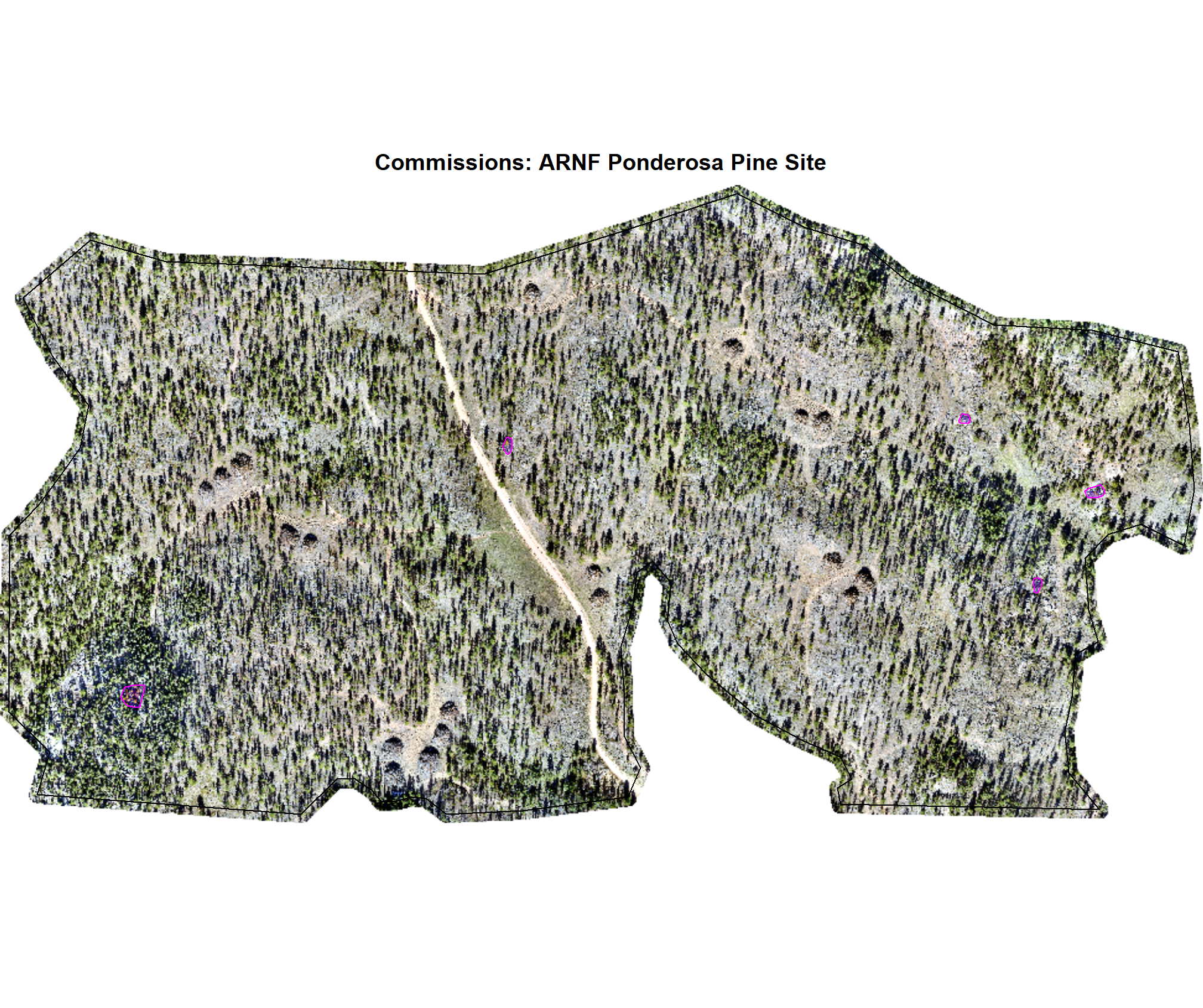
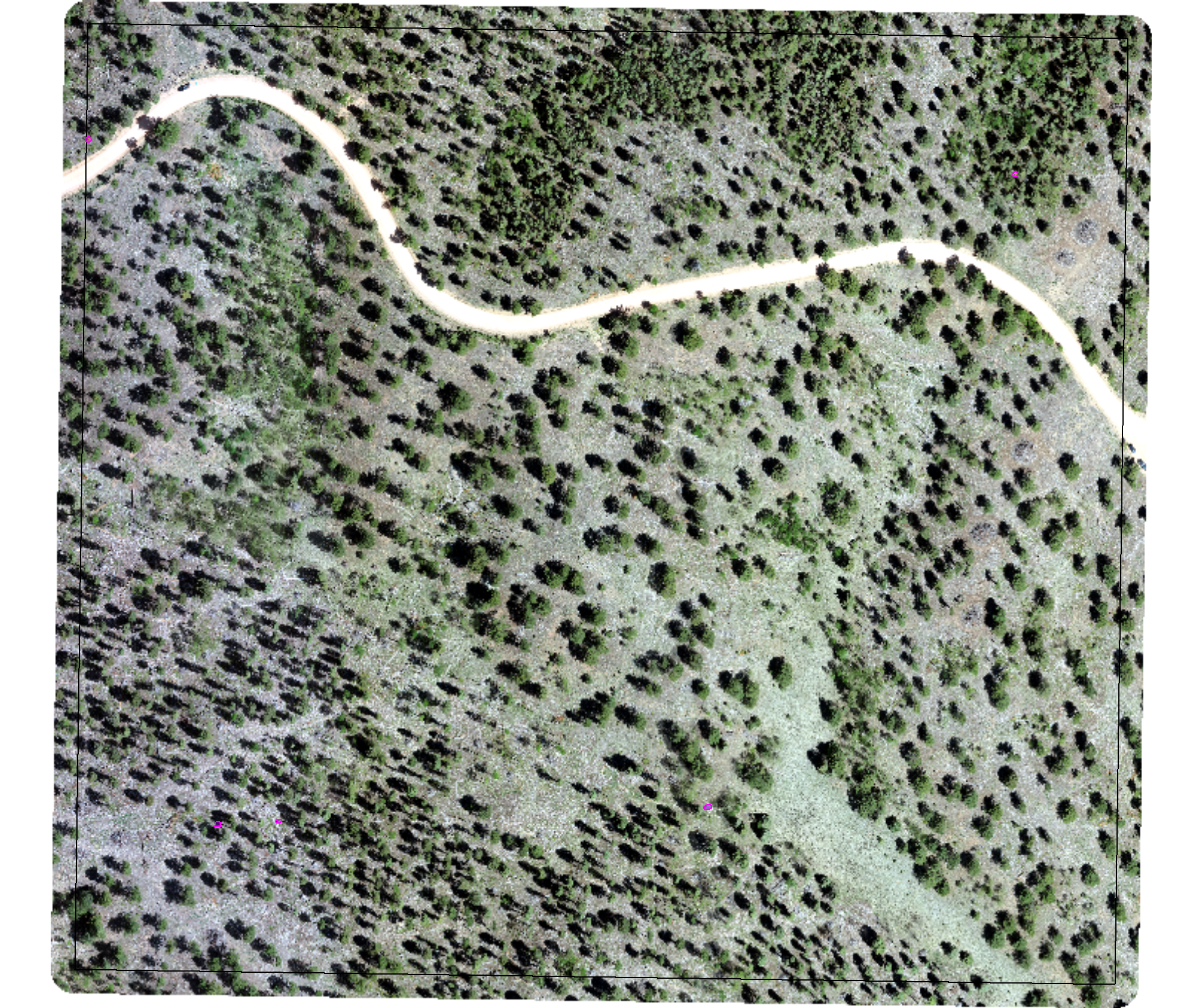
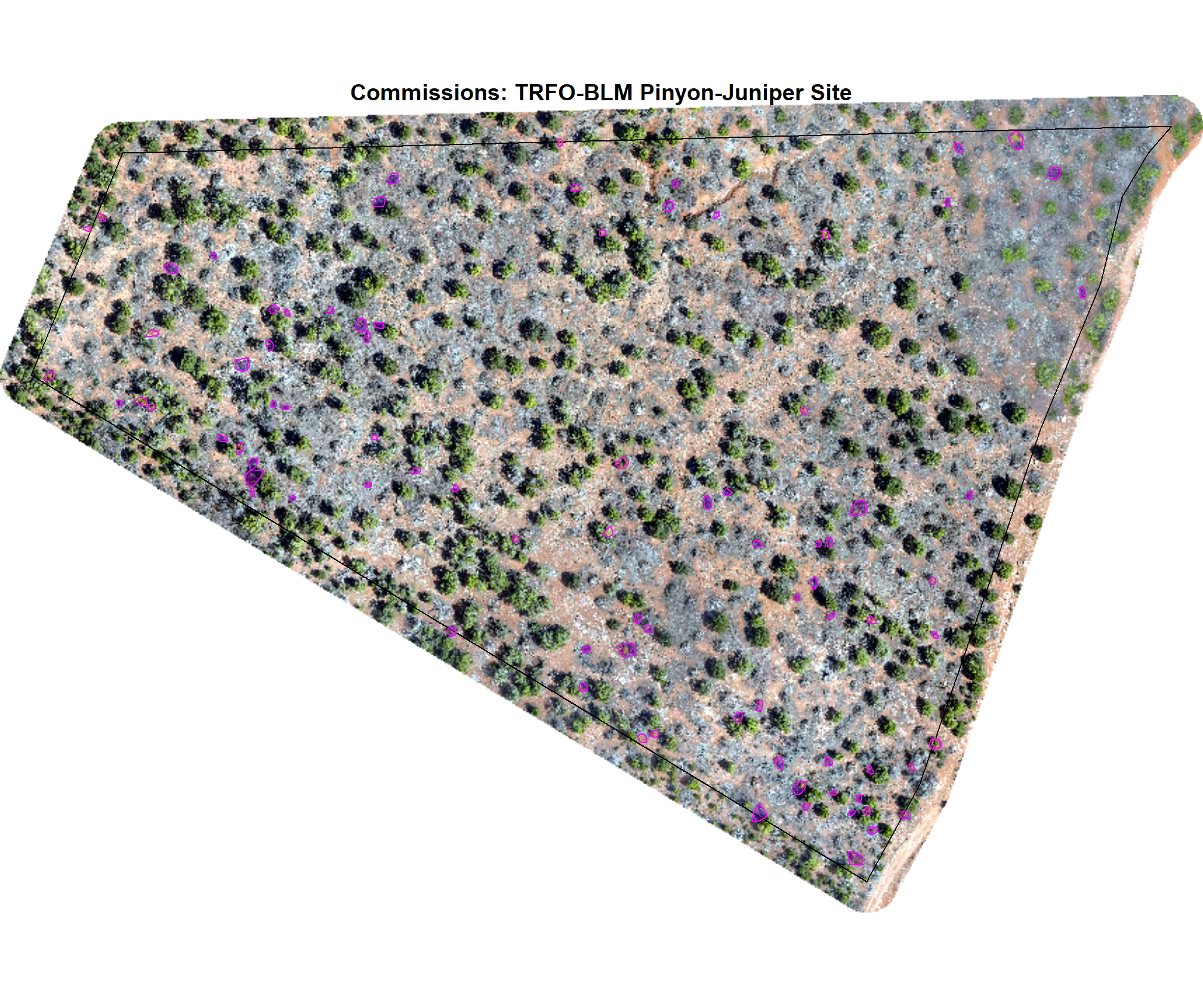
8.4.3.3 Commissions with CHM and RGB

why are these missing?

# map over it 
all_stand_boundary$site_data_lab %>% 
  purrr::map(
    function(x){
    piles <- dbscan_structural_preds[[x]] %>% 
      dplyr::filter(is_in_stand) %>% 
      dplyr::inner_join(
        dbscan_gt_pred_match[[x]] %>% 
        dplyr::filter(match_grp == "commission") %>% 
        dplyr::select(pred_id)
        , by = "pred_id"
      )
    if(nrow(piles)==0){return(NULL)}
    maxh <- all_stand_boundary %>% 
      dplyr::filter(site_data_lab == x) %>% 
      dplyr::slice(1) %>% 
      dplyr::pull(max_ht_m)
    # crop, slice rast
    crp_chm_rast_temp <- chm_rast[[x]] %>% 
      terra::crop(
          piles %>% 
          sf::st_transform(terra::crs(chm_rast[[x]])) %>% 
          terra::vect()
          , mask = T
      )
    
    crp_chm_rast_temp <- crp_chm_rast_temp %>% 
      # slice
      terra::clamp(
        upper = maxh
        , lower = 0
        , values = F
      )
    
    terra_plt_ortho(
      ortho = rgb_rast[[x]]
      , gt_piles = NA
      , pred_piles = piles
      , boundary = stand_boundary[[x]]
      , chm = crp_chm_rast_temp
      , maxh = maxh
      , title = paste0(
        "Commissions: "
        , all_stand_boundary %>% dplyr::filter(site_data_lab==x) %>% dplyr::pull(site)
      )
    )
  })

8.5 Figures for Manuscript

let’s make some figures specifically for the manuscript…these were tacked on after the analysis, so, sorry for the break in sequential flow in the analysis…

Figure 1: study area maps
Figure 2: workflow diagram of proposed method in powerpoint? ;/

8.5.1 Figure 3

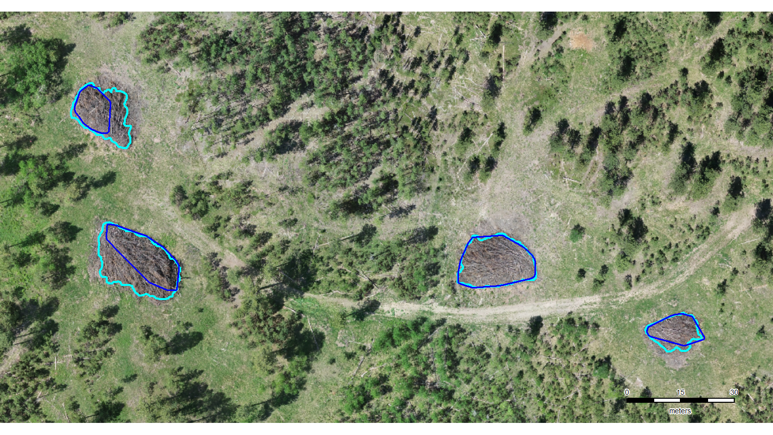
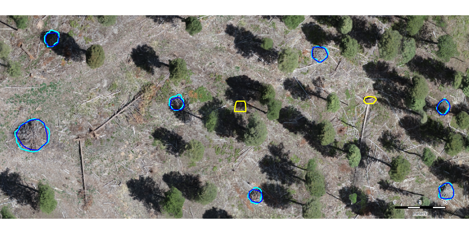
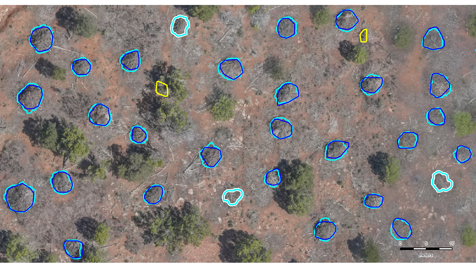
let’s zoom-in on a representative area in each of the four study sites to present detection results (TP, FP, and FN). this will allow users to “see” how the method performed and where it might have struggled

do we have to manually define a sample area in each study site??? probably :|

# manually define aoi
example_aoi <- list(
  "arnf" = 
    dbscan_spectral_preds$arnf %>% 
      dplyr::filter(
        pred_id %in% c(8867,13476,10788) # just need the outermost
      ) %>%
      sf::st_union() %>% 
      sf::st_buffer(30) %>% 
      sf::st_bbox() %>%
      sf::st_as_sfc() %>% 
      sf::st_as_sf() %>% 
    dplyr::mutate(dummy = 1)
  , "bhef" = 
    slash_piles_polys$bhef %>% 
      dplyr::filter(
        pile_id %in% c(
          # 2,3,4 # for vert
          18,19,20,21 # for horz
        ) # just need the outermost
      ) %>%
      sf::st_union() %>% 
      sf::st_buffer(20) %>% 
      sf::st_bbox() %>%
      sf::st_as_sfc() %>% 
      sf::st_as_sf() %>% 
    dplyr::mutate(dummy = 1)
  , "psinf" = 
    slash_piles_polys$psinf %>% 
      dplyr::filter(
        pile_id %in% c(
          # 79, 88, 70 # equal l x w
          84,80,77,78,92 # horz
        ) # just need the outermost
      ) %>%
      sf::st_union() %>% 
      sf::st_buffer(3) %>% 
      sf::st_bbox() %>%
      sf::st_as_sfc() %>% 
      sf::st_as_sf() %>% 
    dplyr::mutate(dummy = 1)
  , "pj" = 
    slash_piles_polys$pj %>% 
      dplyr::filter(
        pile_id %in% c(
          155, 151, 39, 142, 84, 72 # include if want horz 
          # , 40
          # , 5, 6 # include in addition to ^ if want vert
        ) # just need the outermost
      ) %>%
      sf::st_union() %>% 
      sf::st_buffer(0.8) %>% 
      sf::st_bbox() %>%
      sf::st_as_sfc() %>% 
      sf::st_as_sf() %>% 
    dplyr::mutate(dummy = 1)
)

what is the area of each?

example_aoi %>% 
  purrr::map_dfr(
    \(x)
    sf::st_area(x) %>% as.numeric()
  ) %>% 
  tidyr::pivot_longer(dplyr::everything()) %>% 
  dplyr::mutate(value= scales::comma(value/10000, accuracy = 0.01)) %>% 
  kableExtra::kbl(caption = "example AOI area", col.names = c("area short name", "hectares")) %>% 
  kableExtra::kable_styling()

Table 8.5: example AOI area
area short name	hectares
arnf	8.07
bhef	2.50
psinf	0.38
pj	0.46

we could use our ggplot2 based ortho_plt_fn() function to get the RGB basemap for the aoi which we’ll overlay the reference and predictions on…

…but the only reason to do this would be to use patchwork to create a tiled figure that combines all of the example areas from the four study sites. since we are already doing manual stuff, we’re just going to generate the images using the fast-plotting of terra, save them, and then combine them in powerpoint (which will also be not much fun but maybe AI can align since it’s AI and all?). update, AI in powerpoint did not align the images worth a darn. the result looked like what would be generated by a first-time powerpoint user with zero clue about creating visually appealing graphics (small images haphazardly arranged on the slide, comic sans text overlapping and placed partially behind images…). i manually organized the images in powerpoint to make the image for the manuscript that looked decent. one challenge was working with different sized/dimensions example area images.

# high contrast pal
# neon_colors <- c("cyan", "magenta", "gold", "royalblue")
# neon_colors <- c("cyan", "darkorchid", "gold", "white")
neon_colors <- c("cyan", "blue", "yellow", "white")
# neon_colors <- c("cyan", "orange", "gold", "royalblue")
# neon_colors <- c("cyan", "chartreuse", "firebrick", "deepskyblue")
names(neon_colors) <- c("reference", "correct prediction (TP)", "incorrect detection (FP)", "omitted (FN)")
terra_plt_gt_pred_match <- function(nm, seg_mthd = "dbscan") {
  # grDevices::jpeg("../data/psinf_stand_rgb.jpeg", width = 8, height = 8, units = "in", res = 300)
  # mar = c(bottom, left, top, right)
  rgb_temp <- rgb_rast[[nm]] %>% 
    terra::crop(
      example_aoi[[nm]] %>% terra::vect()
    )
  terra::plotRGB(rgb_temp) #, stretch = "lin") #, mar=c(2, 0.5, 3.5, 0.2))
  # all reference piles 
  gt_temp <- slash_piles_polys[[nm]] %>% 
    dplyr::filter(is_in_stand) %>% 
    sf::st_intersection(example_aoi[[nm]])
  # dplyr::glimpse(gt_temp)
  
  # all pred piles 
  if(seg_mthd=="watershed"){
    pred_temp <- watershed_spectral_preds[[nm]] %>% 
      dplyr::filter(is_in_stand) %>% 
      sf::st_intersection(example_aoi[[nm]]) 
  }else{
    pred_temp <- dbscan_spectral_preds[[nm]] %>% 
      dplyr::filter(is_in_stand) %>% 
      sf::st_intersection(example_aoi[[nm]]) 
  }
  # dplyr::glimpse(pred_temp)
  ############################
  # check for FN
  ############################
  if(seg_mthd=="watershed"){
    fn_temp <-
      gt_temp %>% 
      dplyr::inner_join(
        watershed_gt_pred_match[[nm]] %>% 
          dplyr::filter(match_grp == "omission") %>% 
          dplyr::select(pile_id)
        , by = "pile_id"
      )
  }else{
    fn_temp <-
      gt_temp %>% 
      dplyr::inner_join(
        dbscan_gt_pred_match[[nm]] %>% 
          dplyr::filter(match_grp == "omission") %>% 
          dplyr::select(pile_id)
        , by = "pile_id"
      )
  }
  
  if(nrow(fn_temp)>0){
    # add pile boundaries
    terra::plot(
      terra::vect(fn_temp)
      , add = T
      , border = neon_colors[4] # "royalblue"
      , col = NA, lwd = 5
    )  
  }
  ############################
  # add GT
  ############################
  # add pile boundaries
  terra::plot(
    terra::vect(gt_temp)
    , add = T
    , border = neon_colors[1] # "cyan"
    , col = NA, lwd = 2
  )
  ############################
  # check for FP
  ############################
  if(seg_mthd=="watershed"){
    fp_temp <-
      pred_temp %>% 
      dplyr::inner_join(
        watershed_gt_pred_match[[nm]] %>% 
          dplyr::filter(match_grp == "commission") %>% 
          dplyr::select(pred_id)
        , by = "pred_id"
      )
  }else{
    fp_temp <-
      pred_temp %>% 
      dplyr::inner_join(
        dbscan_gt_pred_match[[nm]] %>% 
          dplyr::filter(match_grp == "commission") %>% 
          dplyr::select(pred_id)
        , by = "pred_id"
      )
  }
  
  if(nrow(fp_temp)>0){
    # add pile boundaries
    terra::plot(
      terra::vect(fp_temp)
      , add = T
      , border = neon_colors[3] # "gold"
      , col = NA, lwd = 2
    )  
  }
  ############################
  # add TP
  ############################
  if(seg_mthd=="watershed"){
    tp_temp <-
      pred_temp %>% 
      dplyr::inner_join(
        watershed_gt_pred_match[[nm]] %>% 
          dplyr::filter(match_grp == "true positive") %>% 
          dplyr::select(pred_id)
        , by = "pred_id"
      )
  }else{
    tp_temp <-
      pred_temp %>% 
      dplyr::inner_join(
        dbscan_gt_pred_match[[nm]] %>% 
          dplyr::filter(match_grp == "true positive") %>% 
          dplyr::select(pred_id)
        , by = "pred_id"
      )
  }
  
  if(nrow(tp_temp)>0){
    # add pile boundaries
    terra::plot(
      terra::vect(tp_temp)
      , add = T
      , border = neon_colors[2] # "magenta"
      , col = NA, lwd = 1.8
    )
  }
  # # main title top: "side = 3", line = 1
  # mtext(
  #   all_stand_boundary %>% 
  #     sf::st_drop_geometry() %>% 
  #     dplyr::filter(site_data_lab == nm) %>%
  #     dplyr::pull(site_full_lab)
  #   # "Pike and San Isabel National Forest (PSINF)"
  #   , side = 3, line = 1.5, cex = 0.9, font = 2
  # )
  # # sub title top: "side = 3", line = 1
  # mtext(
  #   paste0(
  #     all_stand_boundary %>% 
  #     sf::st_drop_geometry() %>% 
  #     dplyr::filter(site_data_lab == nm) %>% 
  #     dplyr::mutate(
  #       site_area_ha = scales::comma(site_area_ha, suffix = " ha treatment unit", accuracy = 0.1)
  #     ) %>% 
  #     dplyr::pull(site_area_ha)
  #     , " | "
  #     , psinf_slash_piles_polys %>% dplyr::filter(is_in_stand) %>% nrow() %>% scales::comma(accuracy = 1, suffix = " validation slash piles")
  #   )
  #   , side = 3, line = 0.5, cex = 0.7
  # )
  # 5. Add scale and north arrow
  e_temp <- terra::ext(rgb_temp)
  # 3. Define a position BELOW the minimum Y-coordinate (ymin)
  # Subtracting a small value moves it into the bottom margin
  scale_x_temp <- e_temp$xmin
  scale_y_temp <- e_temp$ymin - ( (e_temp$ymax - e_temp$ymin) * 0.025 ) # 8% below the image
  # ?terra::sbar
  # have to define the scale bar distance
  clean_d_temp <- ceiling((terra::ncol(rgb_temp)*terra::res(rgb_temp)[1]*0.10)/10)*10
  terra::sbar(
    d = clean_d_temp
    , xy = "bottomright"
    # , xy = c(scale_x_temp, scale_y_temp)
    , type = "bar"
    , divs = 5
    , below = "meters"
    , labels = c(0, round(clean_d_temp/2), clean_d_temp)
    , adj = c(0.5, -1.5) # adjust label pos c(horz,vert)
    , cex = 0.45
    # , xpd = T
  )
  # # terra::north(xy = "topright", type = 1, cex = 0.6)
  # grDevices::dev.off()
  # Capture the plot as an object
  grDevices::recordPlot()
}
# do it
example_aoi_plt <- 
  all_stand_boundary$site_data_lab %>% 
  purrr::set_names() %>% 
  purrr::map(terra_plt_gt_pred_match)

# do it again
example_aoi_plt_wshed <- 
  all_stand_boundary$site_data_lab %>% 
  purrr::set_names() %>% 
  purrr::map(\(x) terra_plt_gt_pred_match(nm=x, seg_mthd = "watershed"))

save a color palette for future use

# scales::show_col(neon_colors)
# custom ggplot
neon_colors %>% 
  tibble::enframe() %>% 
  dplyr::mutate(
    x=dplyr::row_number()
    , y = 1
    # x = rep(c(0,1),2)
    # , y = c(0,0,1,1)
    , name = stringr::str_wrap(name, width = 9)
    , zzz = c("black","white","black","black")
  ) %>% 
  ggplot2::ggplot(neon_data, mapping = ggplot2::aes(x = x, y = y, fill = value)) +
  ggplot2::geom_tile(color = "gray", lwd = 1) +
  ggplot2::geom_text(
    mapping = ggplot2::aes(label = name, color = zzz)
    , fontface = "bold"
    , size = 6
  ) +
  ggplot2::scale_fill_identity() +
  ggplot2::scale_color_identity() +
  ggplot2::theme_void() +
  ggplot2::theme(aspect.ratio = 0.2)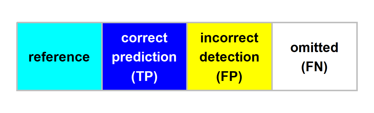

plot them one at a time with custom sizes

8.5.1.1 ARNF

# names(example_aoi_plt)
# grDevices::jpeg("../data/arnf_example_aoi.jpeg", width = 8, height = 4, units = "in", res = 300)
grDevices::replayPlot(example_aoi_plt[["arnf"]])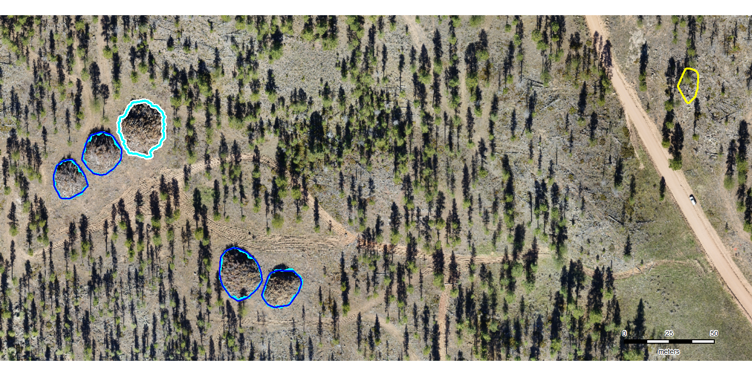

# grDevices::dev.off()

8.5.1.2 BHEF

# names(example_aoi_plt)
# grDevices::jpeg("../data/bhef_example_aoi.jpeg", width = 8, height = 4.5, units = "in", res = 300)
grDevices::replayPlot(example_aoi_plt[["bhef"]])

# grDevices::dev.off()

8.5.1.3 PSINF

# names(example_aoi_plt)
# grDevices::jpeg("../data/psinf_example_aoi.jpeg", width = 8, height = 4, units = "in", res = 300)
grDevices::replayPlot(example_aoi_plt[["psinf"]])

# grDevices::dev.off()

8.5.1.4 TRFO-BLM

# names(example_aoi_plt)
# grDevices::jpeg("../data/pj_example_aoi.jpeg", width = 8, height = 4.5, units = "in", res = 300)
grDevices::replayPlot(example_aoi_plt[["pj"]])

# grDevices::dev.off()