Section 7 Method Predictions
We are finally ready to make predictions using our proposed training-free, rules-based methodology for identifying slash piles from UAS data with a structural and spectral data fusion approach. To this point we have:
- Provided a data overview: here and here
- Processed the UAS point cloud
- Demonstrated our geometry-based slash pile detection methodology
- Demonstrated our spectral refinement (i.e. data fusion) methodology
- and Reviewed how we will evaluate our method
In this section, we’ll implement the proposed geometric, rules-based slash piled detection methodology on our experimental sites using our data fusion approach which utilizes both structural data (i.e. CHM) and spectral RGB data across the four study sites. The integration of spectral data in our data fusion approach allows for less restrictive structural settings, while the absence of spectral filtering would necessitate stricter size and geometric thresholds to minimize false positive predictions. We only test the data fusion method here because the spectral data from imagery is foundational to UAS-DAP point cloud data. That is, aerial imagery is the raw input data used to generate the aerial point cloud data which represents structure in 3D space in UAS-DAP workflows.
7.1 Size and Geometric Parameter Settings
Our geometric, rules-based methodology uses input CHM data and user-defined thresholds for size (height and area) and 2D pile footprint shape regularity (convexity and circularity). The expected height and area search range for slash piles should be based on the pile construction prescription and potentially adjusted based on a sample of field-measured values after treatment completion whether these are a sample of empirical measurements or rough estimates based on visual observation of pile construction outcomes post-treatment. These thresholds define the search space using the CHM data and refine candidate segments to yield final pile predictions.
Here, we review the pile construction prescription (if available) and supplemental visual observational information for each study site and set the size and geometric thresholds for our structural pile detection methodology.
The study site prescriptions can be reviewed here
7.1.1 PSINF Mixed Conifer Site
While the silvicultural prescription provides no specific details regarding pile construction, the management objective to create a wildfire-resilient post-treatment structure suggests that piles were likely located in open spaces away from residual trees. This spacing might enhance the ability of our detection methodology by reducing structural interference from the canopy, regardless of the variations in pile size. Anecdotal feedback from post-treatment site walkthroughs further informs our structural parameters, indicating that hand-piles were generally well-constructed to facilitate efficient prescribed burning and approximately 1.5 m by 1.5 m (5 ft by 5 ft) in size. Mechanical piles at the landings maintained a roughly circular form but were significantly larger, with widths comparable to two or three work vehicles and a taller height than the vehicle.
7.1.2 TRFO-BLM Pinyon-Juniper Site
The silvicultural prescription for the TRFO-BLM site includes exact pile construction minimum dimensions of 1.5 m (5 ft) in length, width, and height, which establishes an expected minimum pile area of approximately 2.3 square meters. While these guidelines focus on compact construction to facilitate consumption during burning, the lack of an explicit maximum size requires the use of anecdotal feedback to determine upper thresholds for our detection methodology. Site managers reported that piles were often larger than expected and “messy” (indicating more irregular footprints than expected). Despite the prescribed residual forest structure being characterized by open interspaces with uniform gaps between trees, the anecdotal observation that piles were frequently constructed too close to residual trees introduces a potential challenge for automated detection. This proximity may cause the structural and spectral signatures of the piles to merge with the surrounding canopy.
7.1.3 BHEF Ponderosa Pine Site
While the silvicultural prescription for the BHEF site defines no specific pile construction parameters, the treatment resulted exclusively in mechanical piles located at landings without additional hand piles. Onsite observations indicated that these piles are gernerally very large and lack a standardized shape or form. For example, some piles were circular and piled high vertically while others were shorter (around DBH) with elongated oval footprints. We established detection thresholds by using familiar anchors to contextualize scale, such as the dimensions of our work truck. Ground-based cell phone images and an aerial UAS photo capturing the truck parked next to one of the largest piles confirmed that some piles reached the scale of a small-sized, one story American single-family home. We used these onsite observations and truck- and house-sized estimates to set high minimum area and height thresholds to isolate the piles from other features. Because these large dimensions may structurally resemble the residual tree groups, spectral information may be key to ensuring the detection accuracy of our method by filtering out false positive predictions from the structural detection.
7.1.4 ARNF Ponderosa Pine Site
While the silvicultural prescription for the ARNF site defines no specific pile construction parameters, it specifies that all residual waste was mechanically piled at landings for future prescribed burning. Onsite observations indicated that these mechanical piles are uniformly massive and generally circular. The piles were also compact and vertical in structure with limited horizontal sprawl, a construction form that will likely increase consumption efficiency during prescribed burning. Some landings contained clusters of two to five individual piles. To calibrate our detection methodology for these large-scale features, we used cell phone photos taken from the ground during site walkthroughs to compare the piles against a lifted Dodge Ram 2500 Mega Cab turbo diesel. By using this vehicle as a known physical anchor, we estimated that the piles were often at least 2-3 the truck’s height of approximately 2.4 m (8 ft), with footprints significantly exceeding the 16.7 to 26.7 square meters of a standard parking space. These dimensional estimates allow us to set relatively large minimum area and height thresholds for our detection methodology to ensure the exclusion of smaller detected objects like trees or boulders since no small hand piles were expected.
7.1.5 Study Paremeter Settings
First, we’re going to make the resolution on the CHM raster for the machine site a bit more coarse since the target object size is larger and we shouldn’t need such fine-grain detail. Also, aggregating the raster to a coarser resolution should help to smooth out some of the noise in fine-grain CHM data which may be necessary for detecting small elevational changes necessary to detect much smaller hand piles.
agg_chm_res_m <- 0.15
# bhef_chm_rast
fnm_temp <- file.path("../data/BHEF_202306/", paste0("bhef_chm_rast_",agg_chm_res_m,"m.tif"))
if(!file.exists(fnm_temp)){
  rast_temp <- bhef_chm_rast
  remove(bhef_chm_rast)
  gc()
  bhef_chm_rast <- cloud2trees:::adjust_raster_resolution(
    raster_object = rast_temp
    , target_resolution = agg_chm_res_m
    , fun = max # max for CHM
    , resample_method = "bilinear"
    , ofile = fnm_temp
  )
  remove(fnm_temp,rast_temp)
  gc()
}else{
  bhef_chm_rast <- terra::rast(fnm_temp)
}
# arnf_chm_rast
fnm_temp <- file.path("../data/ARNF_DiamondView_202510/", paste0("arnf_chm_rast_",agg_chm_res_m,"m.tif"))
if(!file.exists(fnm_temp)){
  rast_temp <- arnf_chm_rast
  remove(arnf_chm_rast)
  gc()
  arnf_chm_rast <- cloud2trees:::adjust_raster_resolution(
    raster_object = rast_temp
    , target_resolution = agg_chm_res_m
    , fun = max # max for CHM
    , resample_method = "bilinear"
    , ofile = fnm_temp
  )
  remove(fnm_temp,rast_temp)
  gc()
}else{
  arnf_chm_rast <- terra::rast(fnm_temp)
}
Set the structural detection parameters based on pile construction prescription and anecdotal feedback from onsite observation
| Parameter | PSINF Mixed Conifer Site | TRFO-BLM Pinyon-Juniper Site | BHEF Ponderosa Pine Site | ARNF Ponderosa Pine Site |
|---|---|---|---|---|
min_ht_m |
1.0 (66% of min. hand pile) | 0.75 (50% of min. hand pile) | 1.25 (slightly < DBH) | 2.4 (truck height) |
max_ht_m |
5.0 (2x truck height) | 3.0 (2x hand pile height) | 6.0 (2.5x truck height) | 9.6 (4x truck height) |
min_area_m2 |
2.0 (90% of min. hand pile) | 2.0 (90% of min. hand pile) | 54.0 (2x parking space) | 54.0 (2x parking space) |
max_area_m2 |
54.0 (2x parking space) | 22.5 (10x min. hand pile) | 486.0 (18x parking space) | 621.0 (23x parking space) |
min_convexity_ratio |
0.65 (strict) | 0.55 (strict) | 0.55 (strict) | 0.55 (strict) |
min_circularity_ratio |
0.5 (strict) | 0.35 (moderate) | 0.0 (no circularity constraint) | 0.3 (moderate) |
for the spectral_weight parameter we can be fairly strict with our spectral filtering across all of these study sites because the piles were generally constructed away from residual trees. As a reminder, the spectral_weight parameter defines the minimum number of the six independent spectral indices that must positively identify a candidate object as non-vegetated to retain it, where increasing the value towards six (6) enforces a stricter consensus to filter out live green vegetation and decreasing it allows for more permissive detection in areas where shadows or canopy overlap may obscure the spectral signature.
| Site | spectral_weight |
Justification |
|---|---|---|
| ARNF | 5 | Located in open landings, these piles have minimal overlap with live canopy; a strict weight ensures that any edge-case vegetation or weeds growing near the piles are effectively excluded. |
| BHEF | 5 | A high consensus threshold is critical here to distinguish massive piles from residual tree groups, as high spectral weight ensures that objects with live green foliage are filtered out of the structural results. |
| TRFO-BLM | 5 | The “heavy intensity uniform thinning treatment” in this pinyon-juniper site which opened up significant space between residual trees likely allows for a strict threshold to reliably remove any candidates which may be green shrubs or low-hanging branches. |
| PSINF | 4 | Because hand piles are often positioned near the residual trees such that many are shadowed by the canopy in the aerial imagery, a slightly lower weight prevents the accidental removal of piles that may be shadowed or have spectral “bleeding” from live tree crowns. |
let’s table that so we have the information
all_stand_boundary <- all_stand_boundary %>%
  dplyr::left_join(
    dplyr::tibble(
      site = c("PSINF Mixed Conifer Site", "TRFO-BLM Pinyon-Juniper Site", "BHEF Ponderosa Pine Site", "ARNF Ponderosa Pine Site")
      , min_ht_m = c(1, 0.75, 1.25, 2.4)
      , max_ht_m = c(5.0, 3.0, 6.0, 9.6)
      , min_area_m2 = c(2.0, 2.0, 54.0, 54.0)
      , max_area_m2 = c(54.0, 22.5, 486.0, 621.0)
      , min_convexity_ratio = c(0.65, 0.55, 0.55, 0.55)
      , min_circularity_ratio = c(0.5, 0.35, 0.0, 0.3)
      , spectral_weight = c(4, 5, 5, 5)
      , chm_res_m = c(
        terra::res(psinf_chm_rast)[1]
        , terra::res(pj_chm_rast)[1]
        , terra::res(bhef_chm_rast)[1]
        , terra::res(arnf_chm_rast)[1]
      )
    )
    , by = "site"
  )
all_stand_boundary %>% dplyr::glimpse()
## Rows: 4
## Columns: 14
## $ site <chr> "ARNF Ponderosa Pine Site", "BHEF Ponderosa Pine…
## $ geometry <GEOMETRY [m]> MULTIPOLYGON (((-794262.3 2..., MULTIPO…
## $ site_area_m2 <dbl> 736062.04, 1031024.64, 174975.91, 51736.28
## $ site_area_ha <dbl> 73.606204, 103.102464, 17.497591, 5.173628
## $ site_data_lab <chr> "arnf", "bhef", "psinf", "pj"
## $ site_full_lab <chr> "Arapahoe and Roosevelt National Forest (ARNF)",…
## $ min_ht_m <dbl> 2.40, 1.25, 1.00, 0.75
## $ max_ht_m <dbl> 9.6, 6.0, 5.0, 3.0
## $ min_area_m2 <dbl> 54, 54, 2, 2
## $ max_area_m2 <dbl> 621.0, 486.0, 54.0, 22.5
## $ min_convexity_ratio <dbl> 0.55, 0.55, 0.65, 0.55
## $ min_circularity_ratio <dbl> 0.30, 0.00, 0.50, 0.35
## $ spectral_weight <dbl> 5, 5, 4, 5
## $ chm_res_m <dbl> 0.15, 0.15, 0.10, 0.10generate a kableExtra table
all_stand_boundary %>%
  sf::st_drop_geometry() %>%
  dplyr::select(-c(
    tidyselect::starts_with("site_area")
    , site_data_lab
    , site_full_lab
  )) %>%
  tidyr::pivot_longer(cols=-site) %>%
  dplyr::mutate(
    value = dplyr::case_when(
      name == "spectral_weight" ~ scales::comma(value,accuracy=1)
      , name %in% c("min_ht_m", "chm_res_m", "min_convexity_ratio", "min_circularity_ratio") ~ scales::comma(value,accuracy=0.01)
      , T ~ scales::comma(value,accuracy=0.1)
    )
  ) %>%
  tidyr::pivot_wider(names_from = site, values_from = value) %>%
  dplyr::rename(parameter = name) %>%
  # kable
  kableExtra::kbl(
    caption = "user-defined thresholds for size and expected pile shape regularity"
    , escape = F
    # , digits = 2
  ) %>%
kableExtra::kable_styling()| parameter | ARNF Ponderosa Pine Site | BHEF Ponderosa Pine Site | PSINF Mixed Conifer Site | TRFO-BLM Pinyon-Juniper Site |
|---|---|---|---|---|
| min_ht_m | 2.40 | 1.25 | 1.00 | 0.75 |
| max_ht_m | 9.6 | 6.0 | 5.0 | 3.0 |
| min_area_m2 | 54.0 | 54.0 | 2.0 | 2.0 |
| max_area_m2 | 621.0 | 486.0 | 54.0 | 22.5 |
| min_convexity_ratio | 0.55 | 0.55 | 0.65 | 0.55 |
| min_circularity_ratio | 0.30 | 0.00 | 0.50 | 0.35 |
| spectral_weight | 5 | 5 | 4 | 5 |
| chm_res_m | 0.15 | 0.15 | 0.10 | 0.10 |
let’s organize our site boundary, ground truth, CHM, and RGB data into lists so we can programmatically iterate through all sites more efficiently
##########################################
# stand_boundary
##########################################
  # suffix
  suffix_temp <- "_stand_boundary"
  # convert to list of objects and remove the suffix from the name in the list
  stand_boundary <-
    all_stand_boundary$site_data_lab %>%
    paste0(suffix_temp) %>%
    base::mget(inherits = T) %>%
    purrr::set_names(~ str_remove(.x, suffix_temp))
  # names(stand_boundary)
  # dplyr::glimpse(stand_boundary)
  # remove
  all_stand_boundary$site_data_lab %>%
    paste0(suffix_temp) %>%
    purrr::map(\(x) remove(list = x,inherits = T))
##########################################
# slash_piles_polys
##########################################
  # suffix
  suffix_temp <- "_slash_piles_polys"
  # convert to list of objects and remove the suffix from the name in the list
  slash_piles_polys <-
    all_stand_boundary$site_data_lab %>%
    paste0(suffix_temp) %>%
    base::mget(inherits = T) %>%
    purrr::set_names(~ str_remove(.x, suffix_temp))
  # names(slash_piles_polys)
  # dplyr::glimpse(slash_piles_polys)
  # remove
  all_stand_boundary$site_data_lab %>%
    paste0(suffix_temp) %>%
    purrr::map(\(x) remove(list = x,inherits = T))
##########################################
# chm_rast
##########################################
  # suffix
  suffix_temp <- "_chm_rast"
  # convert to list of objects and remove the suffix from the name in the list
  chm_rast <-
    all_stand_boundary$site_data_lab %>%
    paste0(suffix_temp) %>%
    base::mget(inherits = T) %>%
    purrr::set_names(~ str_remove(.x, suffix_temp))
  # names(chm_rast)
  # dplyr::glimpse(chm_rast)
  # remove
  all_stand_boundary$site_data_lab %>%
    paste0(suffix_temp) %>%
    purrr::map(\(x) remove(list = x,inherits = T))
##########################################
# rgb_rast
##########################################
  # suffix
  suffix_temp <- "_rgb_rast"
  # convert to list of objects and remove the suffix from the name in the list
  rgb_rast <-
    all_stand_boundary$site_data_lab %>%
    paste0(suffix_temp) %>%
    base::mget(inherits = T) %>%
    purrr::set_names(~ str_remove(.x, suffix_temp))
  # names(rgb_rast)
  # dplyr::glimpse(rgb_rast)
  # remove
  all_stand_boundary$site_data_lab %>%
    paste0(suffix_temp) %>%
    purrr::map(\(x) remove(list = x,inherits = T))
7.2 CHM-based Slash Pile Candidates
Our geometric, rules-based methodology uses input CHM data and user-defined thresholds for size (height and area) and 2D pile footprint shape regularity (convexity and circularity). We defined a function to make the detection from the CHM easy given the parameters we reviewed above: slash_pile_detect()
check the segmentation parameters to be used in each of the DBSCAN and Watershed segmentation methods
segmentation_params_used <-
  all_stand_boundary$site_data_lab %>%
  purrr::set_names() %>%
  purrr::map(
    \(x)
    get_segmentation_params(
        min_ht_m = all_stand_boundary %>% dplyr::filter(site_data_lab==x) %>% dplyr::pull(min_ht_m)
        , max_ht_m = all_stand_boundary %>% dplyr::filter(site_data_lab==x) %>% dplyr::pull(max_ht_m)
        , min_area_m2 = all_stand_boundary %>% dplyr::filter(site_data_lab==x) %>% dplyr::pull(min_area_m2)
        , max_area_m2 = all_stand_boundary %>% dplyr::filter(site_data_lab==x) %>% dplyr::pull(max_area_m2)
        , rast_res_m = terra::res(chm_rast[[x]])[1]
      )
  )
# segmentation_params_used
We’ll get the predictions using both the DBSCAN and Watershed segmentation approaches. Review this section for a refresher on how we use these methods
##################################################
# map over slash_pile_detect for dbscan
##################################################
  # file.names to only run if not already done since it takes a while for all sites
  dir_temp <- "../data"
  if(!dir.exists(dir_temp)){dir.create(dir_temp,showWarnings = F)}
  nmsfx_temp <- "_dbscan_structural_preds.gpkg"
  if(
    !all(file.exists( file.path(dir_temp, paste0(all_stand_boundary$site_data_lab,nmsfx_temp)) ))
  ){
    # map over slash_pile_detect for dbscan
    dbscan_structural_preds <-
      all_stand_boundary$site_data_lab %>%
      purrr::set_names() %>%
      purrr::map(
        \(x)
        slash_pile_detect(
            chm_rast = chm_rast[[x]]
            , seg_method = "dbscan"
            , min_ht_m = all_stand_boundary %>% dplyr::filter(site_data_lab==x) %>% dplyr::pull(min_ht_m)
            , max_ht_m = all_stand_boundary %>% dplyr::filter(site_data_lab==x) %>% dplyr::pull(max_ht_m)
            , min_area_m2 = all_stand_boundary %>% dplyr::filter(site_data_lab==x) %>% dplyr::pull(min_area_m2)
            , max_area_m2 = all_stand_boundary %>% dplyr::filter(site_data_lab==x) %>% dplyr::pull(max_area_m2)
            , min_convexity_ratio = all_stand_boundary %>% dplyr::filter(site_data_lab==x) %>% dplyr::pull(min_convexity_ratio)
            , min_circularity_ratio = all_stand_boundary %>% dplyr::filter(site_data_lab==x) %>% dplyr::pull(min_circularity_ratio)
            , ofile = file.path(dir_temp, paste0(x,nmsfx_temp))
          )
          # purrr::pluck("segs_sf")
        , .progress = T
      )
    # # write
    #   dbscan_structural_preds %>%
    #     purrr::imap(
    #       \(x,nm)
    #       sf::st_write(
    #         obj = x
    #         , dsn = file.path(dir_temp, paste0(nm,nmsfx_temp))
    #         , append = F
    #         , quiet = T
    #       )
    #     )

    # read files
    dbscan_structural_preds <- dbscan_structural_preds %>%
      purrr::map(
        \(x)
        sf::st_read(dsn = x, quiet = T)
      )
  }else{
    # read already done
    dbscan_structural_preds <-
      all_stand_boundary$site_data_lab %>%
      purrr::set_names() %>%
      purrr::map(
        \(x)
        sf::st_read(
          dsn = file.path(dir_temp, paste0(x,nmsfx_temp))
          , quiet = T
        )
      )
  }
  # filter all candidate piles for only those that intersect with the study boundary
  dbscan_structural_preds <-
      all_stand_boundary$site_data_lab %>%
      purrr::set_names() %>%
      purrr::map(
        \(x)
        dplyr::inner_join(
          dbscan_structural_preds[[x]]
          , dbscan_structural_preds[[x]] %>%
            sf::st_intersection(
              stand_boundary[[x]] %>%
              sf::st_transform(sf::st_crs(dbscan_structural_preds[[x]]))
            ) %>%
            sf::st_drop_geometry() %>%
            dplyr::select(pred_id) %>%
            dplyr::mutate(is_in_stand = T)
          , by = "pred_id"
        )
      )
##################################################
# map over slash_pile_detect for watershed
##################################################
  # file.names to only run if not already done since it takes a while for all sites
  dir_temp <- "../data"
  if(!dir.exists(dir_temp)){dir.create(dir_temp,showWarnings = F)}
  nmsfx_temp <- "_watershed_structural_preds.gpkg"
  if(
    !all(file.exists( file.path(dir_temp, paste0(all_stand_boundary$site_data_lab,nmsfx_temp)) ))
  ){
    # map over slash_pile_detect for watershed
    watershed_structural_preds <-
      all_stand_boundary$site_data_lab %>%
      # .[2:4] %>%
      purrr::set_names() %>%
      purrr::map(
        \(x)
        slash_pile_detect(
            chm_rast = chm_rast[[x]]
            , seg_method = "watershed"
            , min_ht_m = all_stand_boundary %>% dplyr::filter(site_data_lab==x) %>% dplyr::pull(min_ht_m)
            , max_ht_m = all_stand_boundary %>% dplyr::filter(site_data_lab==x) %>% dplyr::pull(max_ht_m)
            , min_area_m2 = all_stand_boundary %>% dplyr::filter(site_data_lab==x) %>% dplyr::pull(min_area_m2)
            , max_area_m2 = all_stand_boundary %>% dplyr::filter(site_data_lab==x) %>% dplyr::pull(max_area_m2)
            , min_convexity_ratio = all_stand_boundary %>% dplyr::filter(site_data_lab==x) %>% dplyr::pull(min_convexity_ratio)
            , min_circularity_ratio = all_stand_boundary %>% dplyr::filter(site_data_lab==x) %>% dplyr::pull(min_circularity_ratio)
            , ofile = file.path(dir_temp, paste0(x,nmsfx_temp))
          )
          # purrr::pluck("segs_sf")
        , .progress = T
      )
    # read files
    watershed_structural_preds <- watershed_structural_preds %>%
      purrr::map(
        \(x)
        sf::st_read(dsn = x, quiet = T)
      )
  }else{
    # read already done
    watershed_structural_preds <-
      all_stand_boundary$site_data_lab %>%
      purrr::set_names() %>%
      purrr::map(
        \(x)
        sf::st_read(
          dsn = file.path(dir_temp, paste0(x,nmsfx_temp))
          , quiet = T
        )
      )
  }
  # filter all candidate piles for only those that intersect with the study boundary
  watershed_structural_preds <-
      all_stand_boundary$site_data_lab %>%
      purrr::set_names() %>%
      purrr::map(
        \(x)
        dplyr::inner_join(
          watershed_structural_preds[[x]]
          , watershed_structural_preds[[x]] %>%
            sf::st_intersection(
              stand_boundary[[x]] %>%
              sf::st_transform(sf::st_crs(watershed_structural_preds[[x]]))
            ) %>%
            sf::st_drop_geometry() %>%
            dplyr::select(pred_id) %>%
            dplyr::mutate(is_in_stand = T)
          , by = "pred_id"
        )
      )
let’s summarize the number of structural candidate segments and the area they cover by site
dplyr::bind_rows(
  # watershed
    watershed_structural_preds %>%
    purrr::imap(
      \(x,nm)
      x %>%
        sf::st_drop_geometry() %>%
        dplyr::ungroup() %>%
        dplyr::summarise(
          dplyr::across(
            c(area_m2, volume_m3, max_height_m)
            , .fns = list(
              mean = ~mean(.x,na.rm=T)
              , sd = ~sd(.x,na.rm=T)
              , sum = ~sum(.x,na.rm=T)
            )
          )
          , n = dplyr::n()
        ) %>%
        dplyr::mutate(
          site = all_stand_boundary %>% dplyr::filter(site_data_lab==nm) %>% dplyr::pull(site)
        )
    ) %>%
    dplyr::bind_rows() %>%
    dplyr::mutate(method = "watershed")
  , # dbscan
    dbscan_structural_preds %>%
    purrr::imap(
      \(x,nm)
      x %>%
        sf::st_drop_geometry() %>%
        dplyr::ungroup() %>%
        dplyr::summarise(
          dplyr::across(
            c(area_m2, volume_m3, max_height_m)
            , .fns = list(
              mean = ~mean(.x,na.rm=T)
              , sd = ~sd(.x,na.rm=T)
              , sum = ~sum(.x,na.rm=T)
            )
          )
          , n = dplyr::n()
        ) %>%
        dplyr::mutate(
          site = all_stand_boundary %>% dplyr::filter(site_data_lab==nm) %>% dplyr::pull(site)
        )
    ) %>%
    dplyr::bind_rows() %>%
    dplyr::mutate(method = "dbscan")
) %>%
dplyr::mutate(
  dplyr::across(
    c(tidyselect::ends_with("_sum"),n) # dplyr::where(is.numeric)
    , ~scales::comma(.x,accuracy = 1)
  )
  , dplyr::across(
    dplyr::where(is.numeric)
    , ~scales::comma(.x,accuracy = .1)
  )
  , area_m2_mean = paste0(area_m2_mean, "<br>(",area_m2_sd,")")
  , volume_m3_mean = paste0(volume_m3_mean, "<br>(",volume_m3_sd,")")
  , max_height_m_mean = paste0(max_height_m_mean, "<br>(",max_height_m_sd,")")
) %>%
dplyr::select(
  -tidyselect::ends_with("_sd")
  , -max_height_m_sum
) %>%
dplyr::relocate(site,method,n) %>%
dplyr::arrange(site,method) %>%
kableExtra::kbl(
  caption = "Structurally detected candidate segments by method and study site"
  , col.names = c(
    "site", "method"
    , "# candidates"
    , "area m<sup>2</sup><br>mean (sd)"
    , "area m<sup>2</sup><br>total"
    , "volume m<sup>3</sup><br>mean (sd)"
    , "volume m<sup>3</sup><br>total"
    , "height m<br>mean (sd)"
  )
  , escape = F
  # , digits = 2
) %>%
kableExtra::kable_styling(font_size = 11.5) %>%
kableExtra::collapse_rows(columns = 1, valign = "top")| site | method | # candidates |
area m2 mean (sd) |
area m2 total |
volume m3 mean (sd) |
volume m3 total |
height m mean (sd) |
|---|---|---|---|---|---|---|---|
| ARNF Ponderosa Pine Site | dbscan | 76 |
217.5 (147.6) |
16,533 |
843.8 (500.6) |
64,131 |
8.9 (1.2) |
| watershed | 92 |
183.7 (131.1) |
16,896 |
757.4 (528.3) |
69,677 |
8.9 (1.2) |
|
| BHEF Ponderosa Pine Site | dbscan | 270 |
165.9 (90.3) |
44,802 |
399.6 (258.6) |
107,884 |
5.5 (1.1) |
| watershed | 319 |
150.3 (72.0) |
47,933 |
410.7 (272.3) |
131,019 |
5.5 (1.0) |
|
| PSINF Mixed Conifer Site | dbscan | 188 |
7.6 (7.3) |
1,422 |
10.2 (11.3) |
1,919 |
3.0 (1.3) |
| watershed | 193 |
7.5 (7.2) |
1,450 |
10.3 (11.4) |
1,979 |
3.0 (1.3) |
|
| TRFO-BLM Pinyon-Juniper Site | dbscan | 378 |
8.7 (4.0) |
3,273 |
6.6 (5.6) |
2,477 |
1.6 (0.8) |
| watershed | 377 |
8.6 (4.0) |
3,235 |
6.4 (5.5) |
2,429 |
1.6 (0.8) |
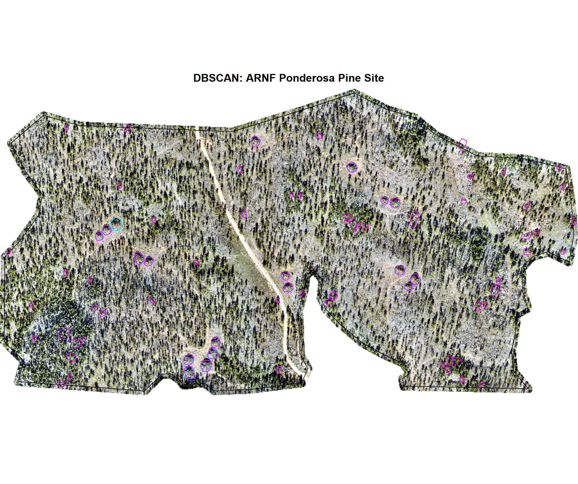
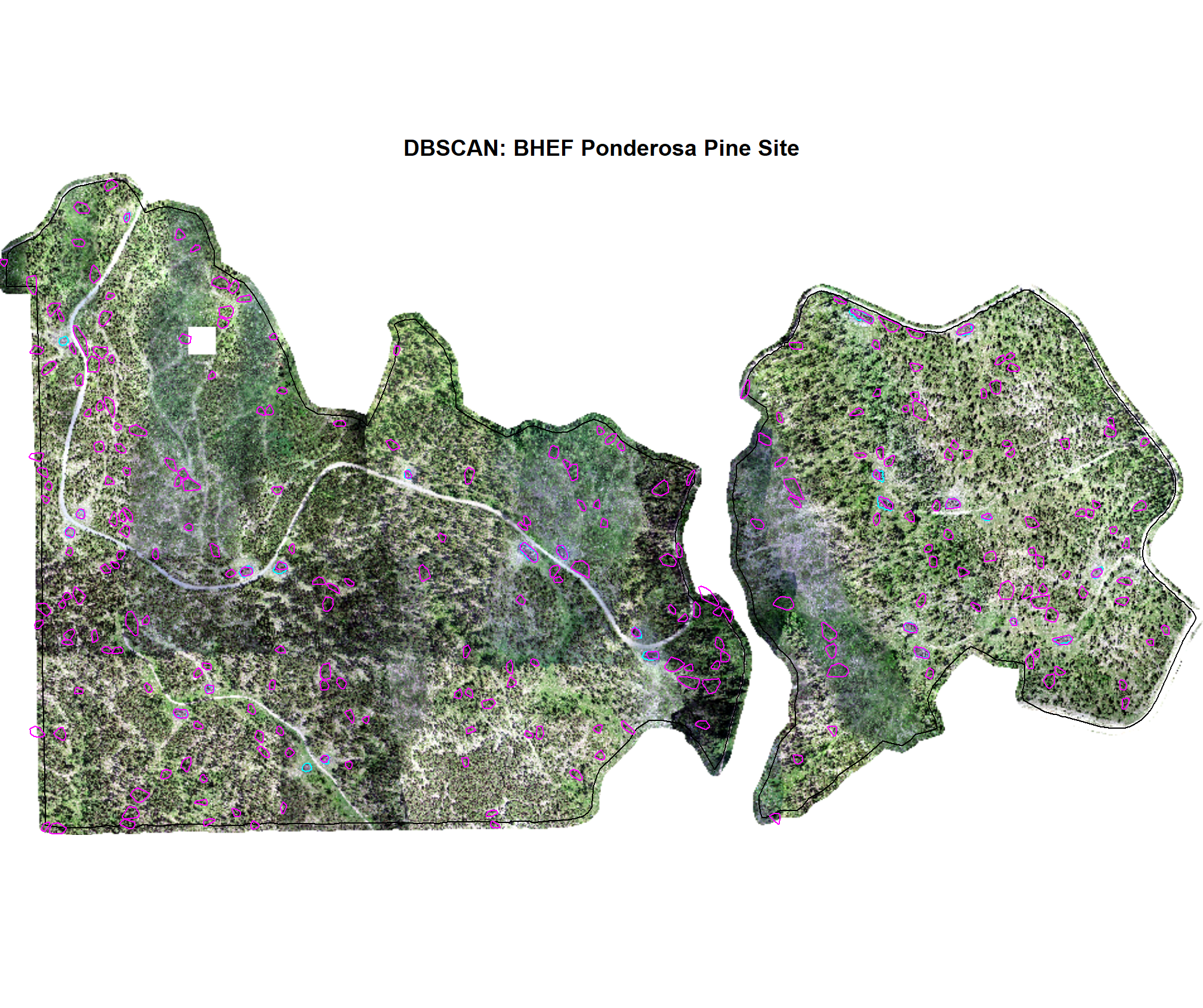
7.2.1 DBSCAN Candidates
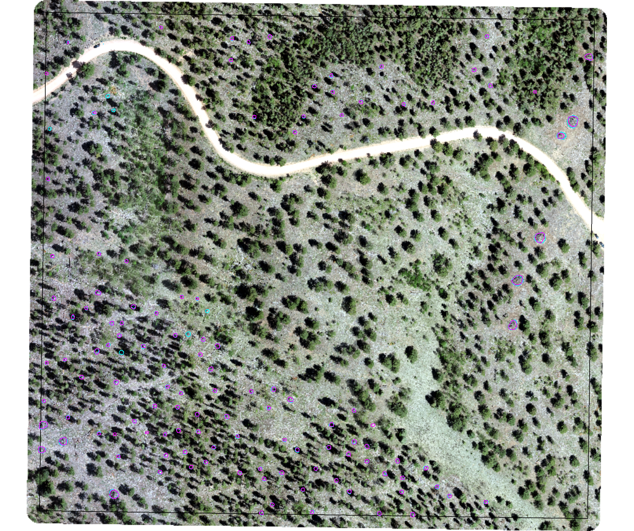
We’ll quickly plot the structurally-detected candidate segments using the DBSCAN method for each study site
# function to plot ortho
terra_plt_ortho <- function(
  ortho
  , gt_piles
  , pred_piles
  , boundary
  , title
) {
  terra::plotRGB(ortho, stretch = "lin")
  terra::plot(
    boundary %>%
      sf::st_transform(terra::crs(ortho)) %>%
      terra::vect()
    , add = T, border = "black", col = NA
    , main = title
  )
  terra::plot(
    gt_piles %>%
      dplyr::filter(is_in_stand) %>%
      sf::st_transform(terra::crs(ortho)) %>%
      terra::vect()
    , add = T, border = "cyan", col = NA, lwd = 1.2
  )
  terra::plot(
    pred_piles %>%
      sf::st_transform(terra::crs(ortho)) %>%
      terra::vect()
    , add = T, border = "magenta", col = NA, lwd = 1.2
  )
}
# map over it
all_stand_boundary$site_data_lab %>%
  purrr::map(
    \(x)
    terra_plt_ortho(
      ortho = rgb_rast[[x]]
      , gt_piles = slash_piles_polys[[x]] %>% dplyr::filter(is_in_stand)
      , pred_piles = dbscan_structural_preds[[x]] %>% dplyr::filter(is_in_stand)
      , boundary = stand_boundary[[x]]
      , title = paste0(
        "DBSCAN: "
        , all_stand_boundary %>% dplyr::filter(site_data_lab==x) %>% dplyr::pull(site)
      )
    )
  )


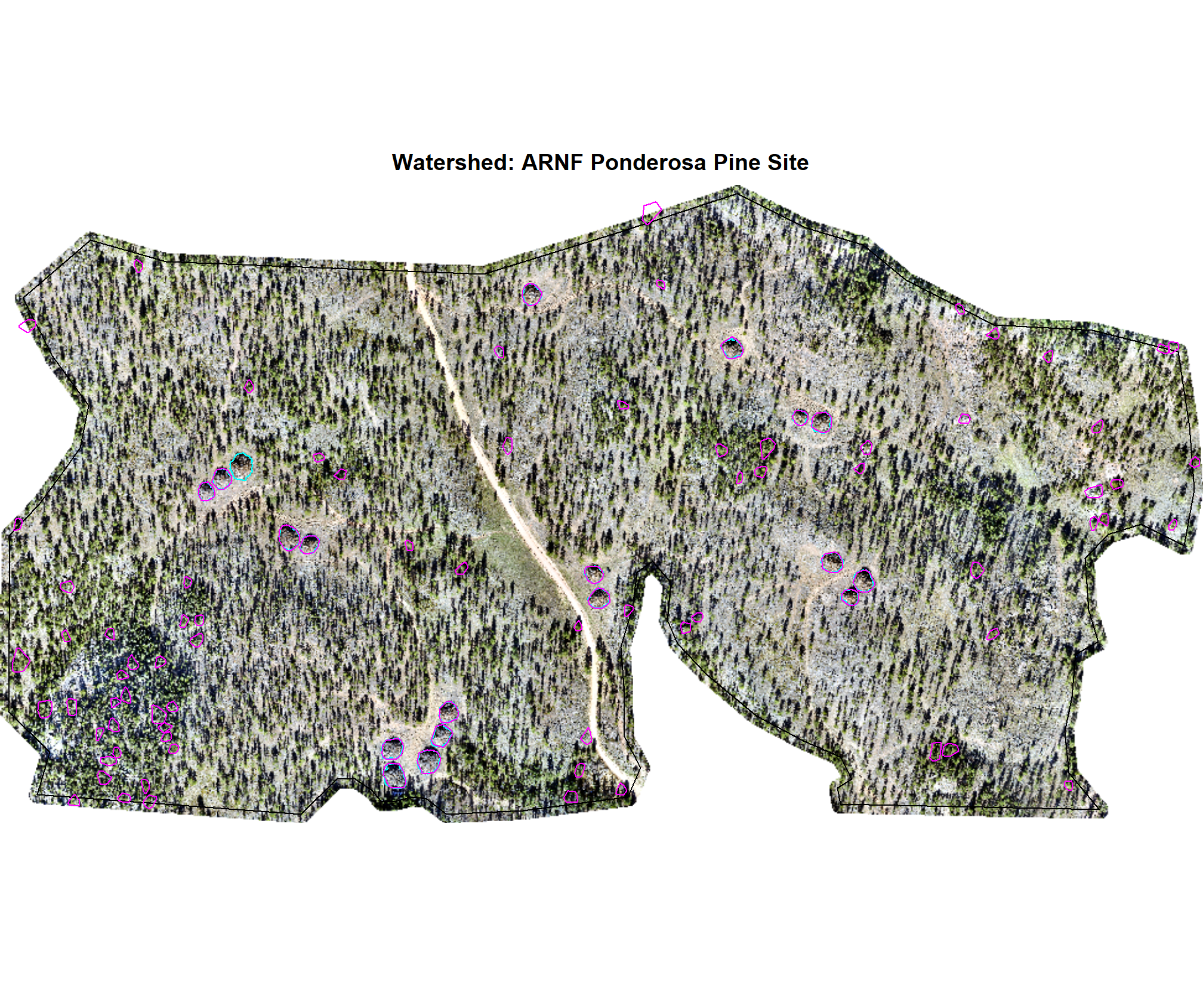
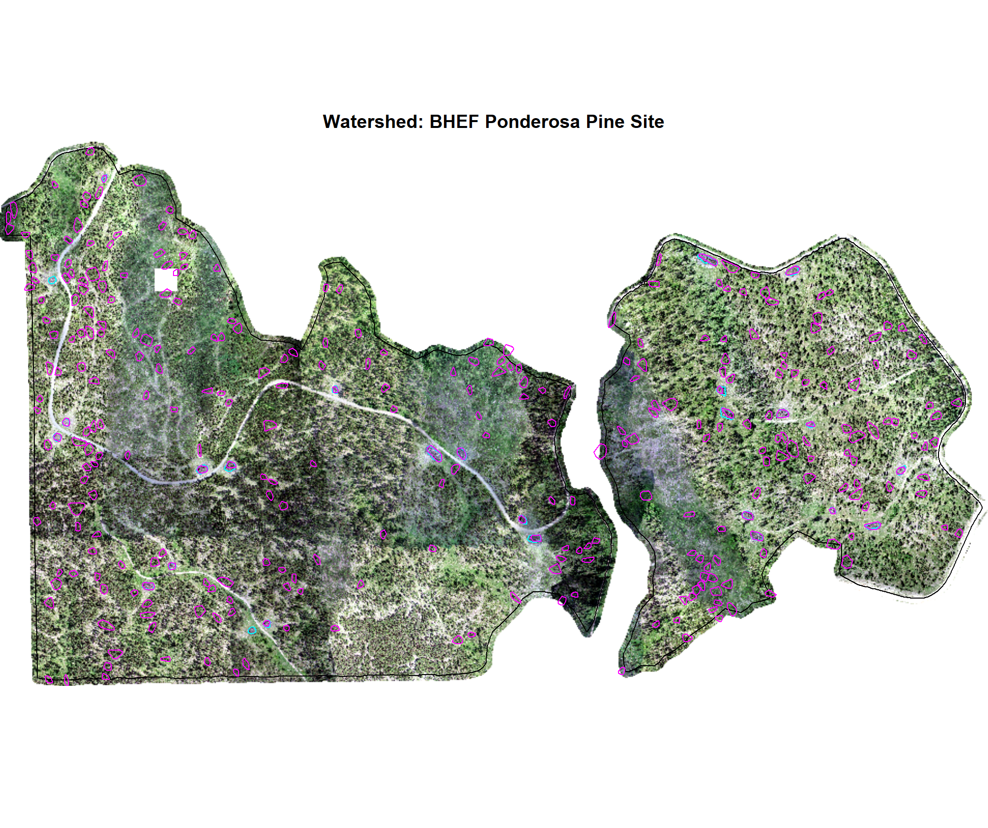
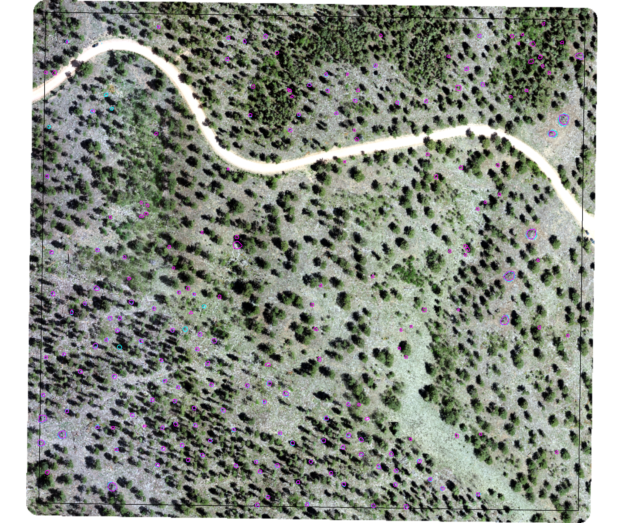
7.2.2 Watershed Candidates
We’ll quickly plot the structurally-detected candidate segments using the Watershed method for each study site
# map over it
all_stand_boundary$site_data_lab %>%
  purrr::map(
    \(x)
    terra_plt_ortho(
      ortho = rgb_rast[[x]]
      , gt_piles = slash_piles_polys[[x]] %>% dplyr::filter(is_in_stand)
      , pred_piles = watershed_structural_preds[[x]] %>% dplyr::filter(is_in_stand)
      , boundary = stand_boundary[[x]]
      , title = paste0(
        "Watershed: "
        , all_stand_boundary %>% dplyr::filter(site_data_lab==x) %>% dplyr::pull(site)
      )
    )
  )

7.3 Spectral Filter Slash Pile Candidates
Now, we’ll apply spectral filtering of the structurally-detected candidate piles using our data fusion approach. As a quick reminder, the spectral filtering functions to distinguish woody debris from live vegetation. We use a spectral voting system using six independent spectral indices derived from RGB data alone. The spectral_weight parameter defines the consensus threshold, requiring a specific number of index thresholds (0-6) required to retain structural candidate piles to generate the final method prediction.
see our parameter setting table above above for the spectral_weight setting which defines how many of the six spectral thresholds must be met for a candidate pile to be retained for final selection as a predicted slash pile.
##################################################
# map over polygon_spectral_filtering for dbscan
##################################################
  # file.names to only run if not already done since it takes a while for all sites
  dir_temp <- "../data"
  if(!dir.exists(dir_temp)){dir.create(dir_temp,showWarnings = F)}
  nmsfx_temp <- "_dbscan_spectral_preds.gpkg"
  if(
    !all(file.exists( file.path(dir_temp, paste0(all_stand_boundary$site_data_lab,nmsfx_temp)) ))
  ){
    # map over polygon_spectral_filtering for dbscan
    dbscan_spectral_preds <-
      all_stand_boundary$site_data_lab %>%
      # .[1:2] %>%
      purrr::set_names() %>%
      # map_chr returns character bc we'll return file path
      purrr::map_chr(
        function(x) {
          # polygon_spectral_filtering
          safe_polygon_spectral_filtering <- purrr::safely(polygon_spectral_filtering)
          segs_sf <- safe_polygon_spectral_filtering(
              sf_data = dbscan_structural_preds[[x]]
              , rgb_rast = rgb_rast[[x]]
              # define the band index
              , red_band_idx = 1
              , green_band_idx = 2
              , blue_band_idx = 3
              , spectral_weight = all_stand_boundary %>% dplyr::filter(site_data_lab==x) %>% dplyr::pull(spectral_weight)
              , filter_return = F
            )
          if(is.null(segs_sf$result)){
            return(NULL)
          }else{
            segs_sf <- segs_sf$result$segs_sf %>%
              dplyr::mutate(
                spectral_weight = all_stand_boundary %>% dplyr::filter(site_data_lab==x) %>% dplyr::pull(spectral_weight)
              )
          }
          # write
          fpth <- file.path(dir_temp, paste0(x,nmsfx_temp))
          sf::st_write(
            obj = segs_sf
            , dsn = fpth
            , append = F
            , quiet = T
          )
          # return
          return(fpth)
        }
      )
    # read files
    dbscan_spectral_preds <- dbscan_spectral_preds %>%
      purrr::map(
        \(x)
        sf::st_read(dsn = x, quiet = T)
      )
  }else{
    # read already done
    dbscan_spectral_preds <-
      all_stand_boundary$site_data_lab %>%
      purrr::set_names() %>%
      purrr::map(
        \(x)
        sf::st_read(
          dsn = file.path(dir_temp, paste0(x,nmsfx_temp))
          , quiet = T
        )
      )
  }
##################################################
# map over polygon_spectral_filtering for watershed
##################################################
  # file.names to only run if not already done since it takes a while for all sites
  dir_temp <- "../data"
  if(!dir.exists(dir_temp)){dir.create(dir_temp,showWarnings = F)}
  nmsfx_temp <- "_watershed_spectral_preds.gpkg"
  if(
    !all(file.exists( file.path(dir_temp, paste0(all_stand_boundary$site_data_lab,nmsfx_temp)) ))
  ){
    # map over polygon_spectral_filtering for watershed
    watershed_spectral_preds <-
      all_stand_boundary$site_data_lab %>%
      # .[3:4] %>%
      purrr::set_names() %>%
      # map_chr returns character bc we'll return file path
      purrr::map_chr(
        function(x) {
          # polygon_spectral_filtering
          safe_polygon_spectral_filtering <- purrr::safely(polygon_spectral_filtering)
          segs_sf <- safe_polygon_spectral_filtering(
              sf_data = watershed_structural_preds[[x]]
              , rgb_rast = rgb_rast[[x]]
              # define the band index
              , red_band_idx = 1
              , green_band_idx = 2
              , blue_band_idx = 3
              , spectral_weight = all_stand_boundary %>% dplyr::filter(site_data_lab==x) %>% dplyr::pull(spectral_weight)
              , filter_return = F
            )
          if(is.null(segs_sf$result)){
            return(NULL)
          }else{
            segs_sf <- segs_sf$result$segs_sf %>%
              dplyr::mutate(
                spectral_weight = all_stand_boundary %>% dplyr::filter(site_data_lab==x) %>% dplyr::pull(spectral_weight)
              )
          }
          # write
          fpth <- file.path(dir_temp, paste0(x,nmsfx_temp))
          sf::st_write(
            obj = segs_sf
            , dsn = fpth
            , append = F
            , quiet = T
          )
          # return
          return(fpth)
        }
      )
    # read files
    watershed_spectral_preds <- watershed_spectral_preds %>%
      purrr::map(
        \(x)
        sf::st_read(dsn = x, quiet = T)
      )
  }else{
    # read already done
    watershed_spectral_preds <-
      all_stand_boundary$site_data_lab %>%
      purrr::set_names() %>%
      purrr::map(
        \(x)
        sf::st_read(
          dsn = file.path(dir_temp, paste0(x,nmsfx_temp))
          , quiet = T
        )
      )
  }
let’s check out the proportion that were filtered out for each site
dplyr::bind_rows(
  watershed_spectral_preds %>%
    purrr::imap(
      \(x,nm)
      x %>%
        dplyr::ungroup() %>%
        sf::st_drop_geometry() %>%
        dplyr::mutate(
          retained = ifelse(inrange_th_votes>=spectral_weight,"retained","removed")
        ) %>%
        dplyr::count(retained) %>%
        dplyr::mutate(
          pct = (n/sum(n)) %>% scales::percent(accuracy = 0.1)
          , n = scales::comma(n,accuracy=1)
        ) %>%
        tidyr::pivot_wider(names_from = retained, values_from = -retained) %>%
        dplyr::mutate(
          site = all_stand_boundary %>% dplyr::filter(site_data_lab==nm) %>% dplyr::pull(site)
          , method = "watershed"
        )
    ) %>%
    dplyr::bind_rows()
  , dbscan_spectral_preds %>%
    purrr::imap(
      \(x,nm)
      x %>%
        dplyr::ungroup() %>%
        sf::st_drop_geometry() %>%
        dplyr::mutate(
          retained = ifelse(inrange_th_votes>=spectral_weight,"retained","removed")
        ) %>%
        dplyr::count(retained) %>%
        dplyr::mutate(
          pct = (n/sum(n)) %>% scales::percent(accuracy = 0.1)
          , n = scales::comma(n,accuracy=1)
        ) %>%
        tidyr::pivot_wider(names_from = retained, values_from = -retained) %>%
        dplyr::mutate(
          site = all_stand_boundary %>% dplyr::filter(site_data_lab==nm) %>% dplyr::pull(site)
          , method = "dbscan"
        )
    ) %>%
    dplyr::bind_rows()
) %>%
dplyr::relocate(site,method) %>%
dplyr::arrange(site,method) %>%
kableExtra::kbl(
  caption = "Spectrally filtered candidate segments by method and study site"
  , col.names = c(
    "site", "method"
    , "# removed", "# retained"
    , "% removed", "% retained"
  )
  , escape = F
  # , digits = 2
) %>%
kableExtra::kable_styling() %>%
kableExtra::collapse_rows(columns = 1, valign = "top")| site | method | # removed | # retained | % removed | % retained |
|---|---|---|---|---|---|
| ARNF Ponderosa Pine Site | dbscan | 53 | 23 | 69.7% | 30.3% |
| watershed | 66 | 26 | 71.7% | 28.3% | |
| BHEF Ponderosa Pine Site | dbscan | 246 | 24 | 91.1% | 8.9% |
| watershed | 294 | 25 | 92.2% | 7.8% | |
| PSINF Mixed Conifer Site | dbscan | 68 | 120 | 36.2% | 63.8% |
| watershed | 70 | 123 | 36.3% | 63.7% | |
| TRFO-BLM Pinyon-Juniper Site | dbscan | 48 | 330 | 12.7% | 87.3% |
| watershed | 48 | 329 | 12.7% | 87.3% |
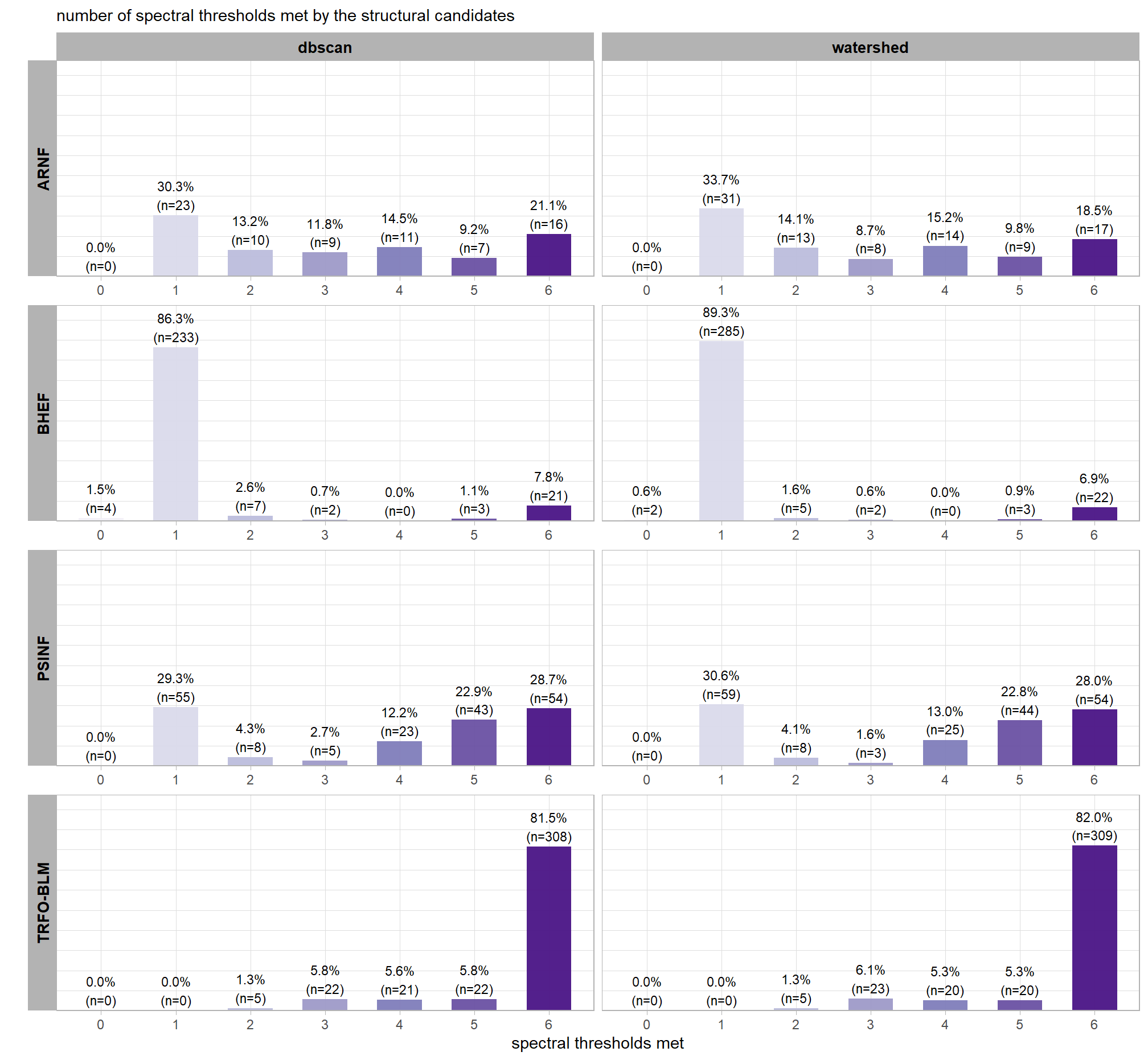
we can look at a distribution of the number of spectral thresholds met by the structural candidates for each site and segmentation method
dplyr::bind_rows(
   dbscan_spectral_preds %>%
      purrr::imap(
        \(x,nm)
        dplyr::tibble(inrange_th_votes = 0:6) %>%
          dplyr::left_join(
            x %>%
              dplyr::ungroup() %>%
              sf::st_drop_geometry() %>%
              dplyr::count(inrange_th_votes)
            , by = "inrange_th_votes"
          ) %>%
          dplyr::mutate(
            site = all_stand_boundary %>% dplyr::filter(site_data_lab==nm) %>% dplyr::pull(site)
            , method = "dbscan"
            , n = dplyr::coalesce(n,0)
          )
      ) %>%
     dplyr::bind_rows()
   , watershed_spectral_preds %>%
    purrr::imap(
      \(x,nm)
      dplyr::tibble(inrange_th_votes = 0:6) %>%
        dplyr::left_join(
          x %>%
            dplyr::ungroup() %>%
            sf::st_drop_geometry() %>%
            dplyr::count(inrange_th_votes)
          , by = "inrange_th_votes"
        ) %>%
        dplyr::mutate(
          site = all_stand_boundary %>% dplyr::filter(site_data_lab==nm) %>% dplyr::pull(site)
          , method = "watershed"
          , n = dplyr::coalesce(n,0)
        )
    ) %>%
    dplyr::bind_rows()
  ) %>%
  dplyr::group_by(site,method) %>%
  dplyr::mutate(
    pct = n/sum(n)
    , inrange_th_votes = ordered(inrange_th_votes)
    , lab = paste0(scales::percent(pct,accuracy=0.1), "\n(n=", scales::comma(n,accuracy=1), ")")
  ) %>%
  dplyr::ungroup() %>%
  dplyr::mutate(site = stringr::word(site)) %>%
  ggplot2::ggplot(
    mapping = ggplot2::aes(x = inrange_th_votes, y = pct, label = lab, fill = inrange_th_votes)
  ) +
  ggplot2::geom_col(
    width = 0.6
    , color = NA, alpha = 0.95
  ) +
  ggplot2::geom_text(color = "black", size = 3, vjust = -0.2) +
  # ggplot2::scale_fill_viridis_d(option = "mako", direction = -1) +
  ggplot2::scale_fill_brewer(palette =  "Purples", direction = 1) +
  ggplot2::scale_y_continuous(
    breaks = seq(0,1,by=0.2)
    , labels = scales::percent
    , expand = ggplot2::expansion(mult = c(0,0.2))
  ) +
  ggplot2::facet_grid(
    rows = dplyr::vars(site)
    , cols = dplyr::vars(method)
    , switch = "y"
    , axes = "all_x"
  ) +
  ggplot2::labs(
    x = "spectral thresholds met", y = "", fill = ""
    , subtitle = "number of spectral thresholds met by the structural candidates"
  ) +
  ggplot2::theme_light() +
  ggplot2::theme(
    legend.position = "none"
    , strip.text = ggplot2::element_text(size = 10, color = "black", face = "bold")
    , axis.text.x = ggplot2::element_text(size = 9)
    , axis.text.y = ggplot2::element_blank()
    , axis.ticks.y = ggplot2::element_blank()
  )
now that we know the breakdown, we can remove the candidates which did not meet the spectral_weight setting
# filter all candidate piles for only those that meet the spectral_weight setting
dbscan_spectral_preds <-
    dbscan_spectral_preds %>%
    purrr::map(
      \(x)
      x %>%
        dplyr::filter(inrange_th_votes>=spectral_weight)
    )
watershed_spectral_preds <-
    watershed_spectral_preds %>%
    purrr::map(
      \(x)
      x %>%
        dplyr::filter(inrange_th_votes>=spectral_weight)
    )
let’s summarize the number of final candidate segments that passed the spectral filtering and the area they cover by site
dplyr::bind_rows(
  # watershed
    watershed_spectral_preds %>%
    purrr::imap(
      \(x,nm)
      x %>%
        sf::st_drop_geometry() %>%
        dplyr::ungroup() %>%
        dplyr::summarise(
          dplyr::across(
            c(area_m2, volume_m3, max_height_m)
            , .fns = list(
              mean = ~mean(.x,na.rm=T)
              , sd = ~sd(.x,na.rm=T)
              , sum = ~sum(.x,na.rm=T)
            )
          )
          , n = dplyr::n()
        ) %>%
        dplyr::mutate(
          site = all_stand_boundary %>% dplyr::filter(site_data_lab==nm) %>% dplyr::pull(site)
        )
    ) %>%
    dplyr::bind_rows() %>%
    dplyr::mutate(method = "watershed")
  , # dbscan
    dbscan_spectral_preds %>%
    purrr::imap(
      \(x,nm)
      x %>%
        sf::st_drop_geometry() %>%
        dplyr::ungroup() %>%
        dplyr::summarise(
          dplyr::across(
            c(area_m2, volume_m3, max_height_m)
            , .fns = list(
              mean = ~mean(.x,na.rm=T)
              , sd = ~sd(.x,na.rm=T)
              , sum = ~sum(.x,na.rm=T)
            )
          )
          , n = dplyr::n()
        ) %>%
        dplyr::mutate(
          site = all_stand_boundary %>% dplyr::filter(site_data_lab==nm) %>% dplyr::pull(site)
        )
    ) %>%
    dplyr::bind_rows() %>%
    dplyr::mutate(method = "dbscan")
) %>%
dplyr::mutate(
  dplyr::across(
    c(tidyselect::ends_with("_sum"),n) # dplyr::where(is.numeric)
    , ~scales::comma(.x,accuracy = 1)
  )
  , dplyr::across(
    dplyr::where(is.numeric)
    , ~scales::comma(.x,accuracy = .1)
  )
  , area_m2_mean = paste0(area_m2_mean, "<br>(",area_m2_sd,")")
  , volume_m3_mean = paste0(volume_m3_mean, "<br>(",volume_m3_sd,")")
  , max_height_m_mean = paste0(max_height_m_mean, "<br>(",max_height_m_sd,")")
) %>%
dplyr::select(
  -tidyselect::ends_with("_sd")
  , -max_height_m_sum
) %>%
dplyr::relocate(site,method,n) %>%
dplyr::arrange(site,method) %>%
kableExtra::kbl(
  caption = "Final, spectrally filtered candidate segments by method and study site"
  , col.names = c(
    "site", "method"
    , "# candidates"
    , "area m<sup>2</sup><br>mean (sd)"
    , "area m<sup>2</sup><br>total"
    , "volume m<sup>3</sup><br>mean (sd)"
    , "volume m<sup>3</sup><br>total"
    , "height m<br>mean (sd)"
  )
  , escape = F
  # , digits = 2
) %>%
kableExtra::kable_styling(font_size = 11.5) %>%
kableExtra::collapse_rows(columns = 1, valign = "top")| site | method | # candidates |
area m2 mean (sd) |
area m2 total |
volume m3 mean (sd) |
volume m3 total |
height m mean (sd) |
|---|---|---|---|---|---|---|---|
| ARNF Ponderosa Pine Site | dbscan | 23 |
371.9 (133.4) |
8,553 |
1,155.3 (608.2) |
26,573 |
7.7 (1.4) |
| watershed | 26 |
326.5 (152.7) |
8,488 |
1,001.2 (640.6) |
26,032 |
7.7 (1.3) |
|
| BHEF Ponderosa Pine Site | dbscan | 24 |
180.8 (82.6) |
4,339 |
174.9 (126.2) |
4,198 |
2.3 (0.6) |
| watershed | 25 |
177.4 (82.7) |
4,434 |
178.2 (124.8) |
4,455 |
2.5 (0.9) |
|
| PSINF Mixed Conifer Site | dbscan | 120 |
8.9 (8.3) |
1,072 |
8.8 (12.6) |
1,054 |
2.2 (0.7) |
| watershed | 123 |
9.0 (8.5) |
1,113 |
9.0 (13.0) |
1,111 |
2.2 (0.7) |
|
| TRFO-BLM Pinyon-Juniper Site | dbscan | 330 |
8.9 (3.9) |
2,935 |
5.5 (3.5) |
1,816 |
1.4 (0.7) |
| watershed | 329 |
8.8 (3.8) |
2,905 |
5.4 (3.3) |
1,785 |
1.4 (0.7) |
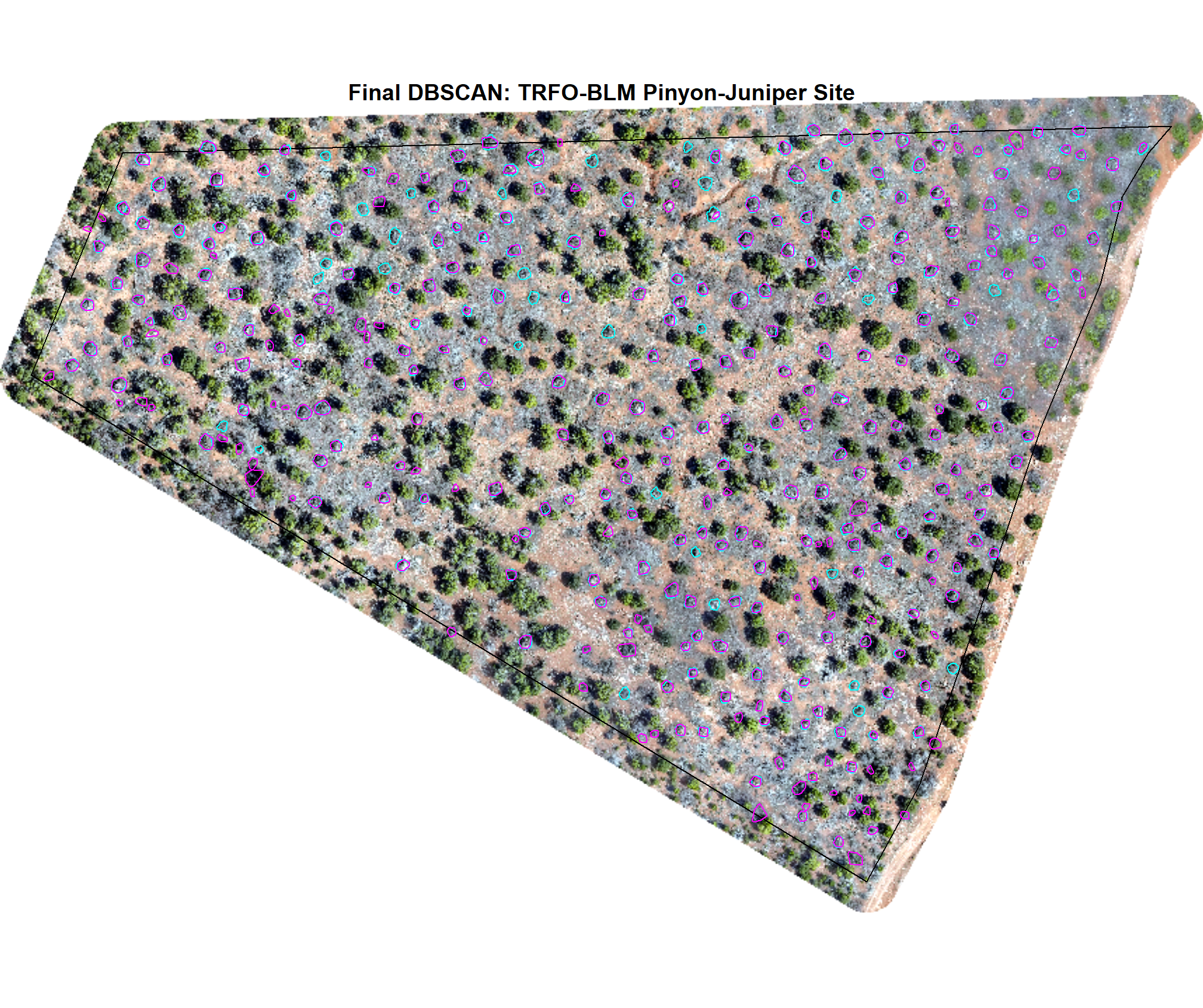
7.3.1 DBSCAN Predictions
We’ll quickly plot the structurally-detected and spectrally filtered candidate segments using the DBSCAN method for each study site
# map over it
all_stand_boundary$site_data_lab %>%
  purrr::map(
    \(x)
    terra_plt_ortho(
      ortho = rgb_rast[[x]]
      , gt_piles = slash_piles_polys[[x]] %>% dplyr::filter(is_in_stand)
      , pred_piles = dbscan_spectral_preds[[x]] %>% dplyr::filter(is_in_stand)
      , boundary = stand_boundary[[x]]
      , title = paste0(
        "Final DBSCAN: "
        , all_stand_boundary %>% dplyr::filter(site_data_lab==x) %>% dplyr::pull(site)
      )
    )
  )

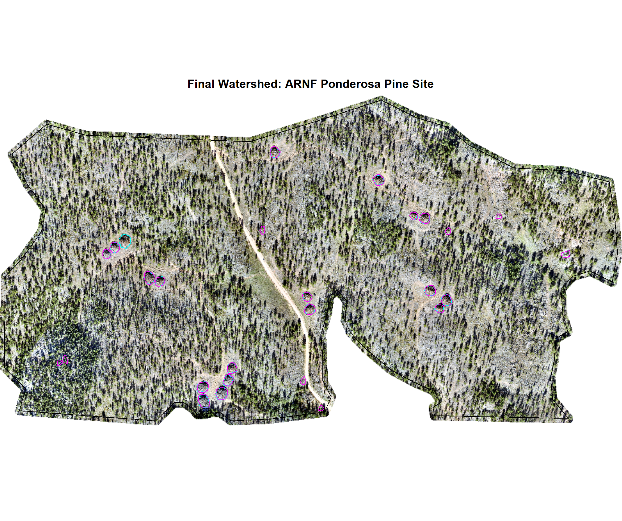
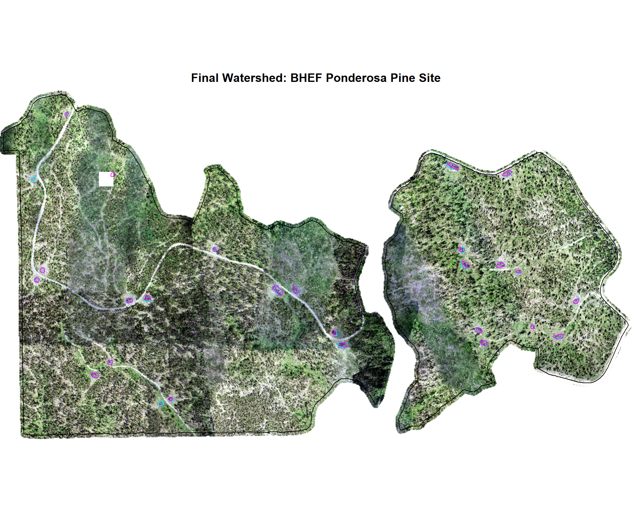
7.3.2 Watershed Predictions
We’ll quickly plot the structurally-detected and spectrally filtered candidate segments using the Watershed method for each study site
# map over it
all_stand_boundary$site_data_lab %>%
  purrr::map(
    \(x)
    terra_plt_ortho(
      ortho = rgb_rast[[x]]
      , gt_piles = slash_piles_polys[[x]] %>% dplyr::filter(is_in_stand)
      , pred_piles = watershed_spectral_preds[[x]] %>% dplyr::filter(is_in_stand)
      , boundary = stand_boundary[[x]]
      , title = paste0(
        "Final Watershed: "
        , all_stand_boundary %>% dplyr::filter(site_data_lab==x) %>% dplyr::pull(site)
      )
    )
  )