Section 4 Geometry-based Slash Pile Detection
In this section, we will demonstrate the geometry-based slash pile detection method which relies upon user-defined thresholds applied to geometric features from a Canopy Height Model (CHM) derived from UAS-DAP point cloud data. Since this is only a demonstration of the method, we will work with only a sample area from one of the study sites which we know includes slash piles. Full evaluation of the methodology will be performed later in the analysis.
We’ll attempt to detect slash piles using raster-based methods with the CHM. These raster-based approaches are simple and efficient but rasterization simplifies/removes some of the rich 3D information in the point cloud. However, raster-based approaches for detecting individual trees in forest stands and coarse woody debris are common.
Here is a section from the draft manuscript:
These geometry-based approaches are supported by the demonstrated successes of object segmentation frameworks for both CWD and individual trees, which consistently provide high detection and quantification accuracy by utilizing rules to define expected target object morphology. Beyond their technical performance, the geometry-based methods utilizing a set of rules offer some key advantages. The inherent traceability of these methods ensures that reporting for regulatory oversight is more transparent and easier to describe compared to the “black box” nature of many model-based approaches. Geometry-based frameworks also do not rely on training datasets and can directly align with the explicit pile construction parameters which are generally known by land managers through silvicultural prescriptions. To address the current lack of automated methods for simultaneously detecting and quantifying slash piles from aerial remote sensing data, our objective in this work is to present a geometry-based approach that uses rules and user-defined thresholds applied to geometric features (such as area, shape, and height) to identify and quantify slash piles from UAS-DAP point cloud data.
Geometric, rules-based object detection methods offer advantages over model-based approaches, primarily because they eliminate the need for extensive training data which might be limited in it’s transferability to unseen conditions. Models are often considered “black boxes” but rules-based methods rely on the inherent physical properties of the target objects themselves. This transparency allows for a high degree of interpretability as every segmentation result can be traced back to specific geometric constraints. Furthermore, this approach aligns perfectly with the expertise of land managers, as the input parameters like minimum height and area thresholds are the physical metrics commonly used in forest inventories and silvicultural prescriptions. By using these intuitive thresholds, the method becomes accessible to managers who possess a good understanding of the landscape they manage.
To attempt to identify slash piles from the CHM/DSM, we can use watershed segmentation or DBSCAN (Density-Based Spatial Clustering of Applications with Noise). Both of these methods are common in segmenting individual trees and coarse woody debris from CHM data.
4.1 Demonstration Area
we’ll focus on an example area that is outside of the study unit boundary but was captured in our UAS data acquisition of the area. This demonstration area also included slash piles which were annotated in the same manner as previously described but did not have height and diameter measurements taken in the field.
# boundary
aoi_boundary <-
  psinf_slash_piles_polys %>%
  dplyr::filter(
    !is_in_stand
    & pile_id %in% c(53,52,63,20,17,11,6,75)
  ) %>%
  sf::st_union() %>%
  sf::st_bbox() %>%
  sf::st_as_sfc() %>%
  sf::st_buffer(1.3, joinStyle = "MITRE") %>%
  sf::st_as_sf() %>%
  dplyr::mutate(dummy=1)
we cropped this section from our original RGB processing, so we’ll get it now
dir_temp <- "../data/PFDP_Data/"
rgb_fnm_temp <- file.path(dir_temp,"aoi_rgb_rast.tif") # what should the compiled rgb be called?
if(!dir.exists(dir_temp)){dir.create(dir_temp, showWarnings = F)}
if(!file.exists(rgb_fnm_temp)){
  #### read RGB data keep only RGB
    aoi_rgb_rast <- terra::rast(
        file.path(
          "f:\\PFDP_Data\\p4pro_images\\P4Pro_06_17_2021_half_half_optimal\\3_dsm_ortho\\2_mosaic"
          , "P4Pro_06_17_2021_half_half_optimal_transparent_mosaic_group1.tif"
        )
      ) %>%
      terra::subset(c(1,2,3))
    # rename bands
    names(aoi_rgb_rast) <- c("red","green","blue")
  # Crop the raster to the rectangular extent of the polygon
  # Specify a filename to ensure the result is written to disk
  crop_rgb_rast_temp <- aoi_rgb_rast %>%
    terra::crop(
      aoi_boundary %>%
        sf::st_union() %>%
        sf::st_buffer(4) %>%
        sf::st_transform(terra::crs(aoi_rgb_rast)) %>%
        terra::vect()
      , mask = T
      , filename =  tempfile(fileext = ".tif")
      , overwrite = TRUE
    )

  ## apply the change_res_fn for our analysis we don't need such finery
  # this takes too long...
  aoi_rgb_rast <- change_res_fn(crop_rgb_rast_temp, my_res=my_rgb_res_m, ofile = rgb_fnm_temp)
  aoi_rgb_rast <- aoi_rgb_rast %>%
    terra::crop(
      aoi_boundary %>%
        sf::st_buffer(2) %>%
        sf::st_transform(terra::crs(aoi_rgb_rast)) %>%
        terra::vect()
      , mask = T
    )
}else{
  aoi_rgb_rast <- terra::rast(rgb_fnm_temp)
  aoi_rgb_rast <- aoi_rgb_rast %>%
    terra::crop(
      aoi_boundary %>%
        sf::st_buffer(2) %>%
        sf::st_transform(terra::crs(aoi_rgb_rast)) %>%
        terra::vect()
      , mask = T
    )
}
# terra::res(aoi_rgb_rast)
# terra::plotRGB(aoi_rgb_rast, stretch = "lin")
we cropped this section from our original CHM processing, so we’ll get it now
dir_temp <- "../data/PFDP_Data/"
chm_fnm_temp <- file.path(dir_temp,"aoi_chm_rast.tif") # what should the compiled chm be called?
if(!dir.exists(dir_temp)){dir.create(dir_temp, showWarnings = F)}
if(!file.exists(chm_fnm_temp)){
  #### read CHM
    aoi_chm_rast <- terra::rast(
        file.path(
          dir_temp
          , "point_cloud_processing_delivery_chm0.1m"
          , "chm_0.1m.tif"
        )
      ) %>%
      terra::subset(1)
  # Crop the raster to the rectangular extent of the polygon
  # Specify a filename to ensure the result is written to disk
  aoi_chm_rast <- aoi_chm_rast %>%
    terra::crop(
      aoi_boundary %>%
        sf::st_union() %>%
        sf::st_buffer(4) %>%
        sf::st_transform(terra::crs(aoi_chm_rast)) %>%
        terra::vect()
      , mask = T
      , filename = chm_fnm_temp
      , overwrite = TRUE
    )

  aoi_chm_rast <- aoi_chm_rast %>%
    terra::crop(
      aoi_boundary %>%
        sf::st_buffer(2) %>%
        sf::st_transform(terra::crs(aoi_chm_rast)) %>%
        terra::vect()
      , mask = T
    )
}else{
  aoi_chm_rast <- terra::rast(chm_fnm_temp)
  aoi_chm_rast <- aoi_chm_rast %>%
    terra::crop(
      aoi_boundary %>%
        sf::st_buffer(2) %>%
        sf::st_transform(terra::crs(aoi_chm_rast)) %>%
        terra::vect()
      , mask = T
    )
}
# terra::res(aoi_chm_rast)
# terra::plot(aoi_chm_rast)
get the piles that intersect with our AOI boundary
# piles
aoi_slash_piles_polys <- psinf_slash_piles_polys %>%
  dplyr::inner_join(
    psinf_slash_piles_polys %>%
      sf::st_intersection(aoi_boundary) %>%
      sf::st_drop_geometry() %>%
      dplyr::select(pile_id)
    , by = "pile_id"
  )
# aoi_slash_piles_polys %>% sf::st_drop_geometry() %>% dplyr::count(is_in_stand)
# ggplot base
aoi_plt_ortho <- ortho_plt_fn(rgb_rast = aoi_rgb_rast, stand = aoi_boundary, buffer = 3)
# aoi_plt_ortho
look at the demonstration area (plots using ggplot2 for maximum customization)
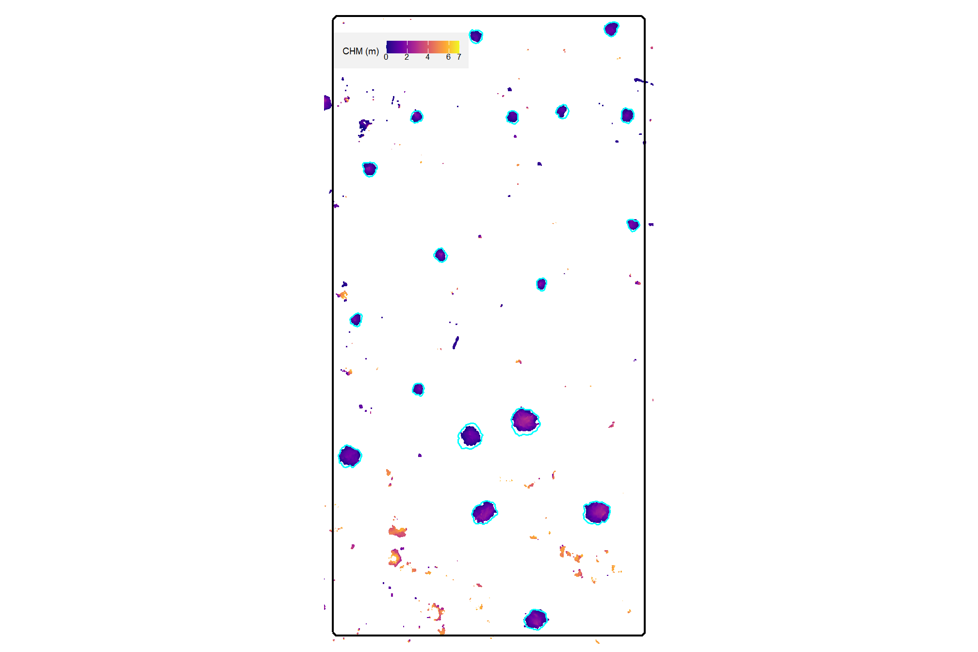
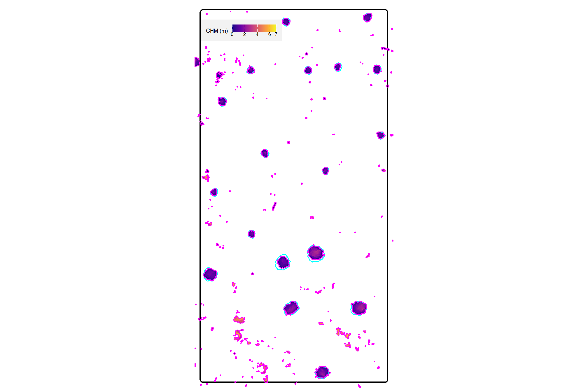
here is the CHM of the example area. can you pick out the slash piles?
plt_aoi_chm <- function(chm, opt="plasma") {
  max_val <- ceiling(terra::minmax(chm)[2]*1.02)
  rng <- c(0,max(max_val,1))
  pretty <- scales::breaks_pretty(n = 4)(rng)

  thrsh <- 0.10 * (max(rng) - min(rng))
  filtered_pretty <- pretty[
    abs(pretty - min(rng)) > thrsh &
    abs(pretty - max(rng)) > thrsh
  ]
  brks <-
    c(
      rng
      , filtered_pretty
    ) %>%
    unique() %>%
    sort()

  chm %>%
    terra::as.data.frame(xy=T) %>%
    dplyr::rename(f=3) %>%
    ggplot2::ggplot() +
    ggplot2::geom_tile(mapping = ggplot2::aes(x=x,y=y,fill=f)) +
    ggplot2::geom_sf(data = aoi_boundary %>% sf::st_buffer(3.8), fill = NA, color = "white", lwd = 0.0) + # so if chm is missing still same size
    ggplot2::geom_sf(data = aoi_boundary, fill = NA, color = "black", lwd = 0.8) +
    # ggplot2::scale_fill_viridis_c(option = opt) +
    ggplot2::scale_fill_viridis_c(option = opt, limits = rng, breaks = brks) +
    ggplot2::labs(fill = "CHM (m)") +
    ggplot2::scale_x_continuous(expand = c(0, 0)) +
    ggplot2::scale_y_continuous(expand = c(0, 0)) +
    ggplot2::theme_void() +
    ggplot2::theme(
      # legend.position = "top"
      legend.position = "inside"
      , legend.position.inside = c(0.05, 0.95)
      , legend.justification.inside = c(0, 1)
      , legend.direction = "horizontal"
      , legend.title = ggplot2::element_text(size = 7)
      , legend.text = ggplot2::element_text(size = 6.5, margin = ggplot2::margin(t = -0.01))
      , legend.key.height = unit(0.35, "cm")
      , legend.key.width = unit(0.4, "cm")
      , legend.background = ggplot2::element_rect(fill = "gray95") #, color = "black")
      , legend.margin = ggplot2::margin(t = 6, r = 7, b = 6, l = 7, unit = "pt")
    )
}
plt_aoi_chm(aoi_chm_rast)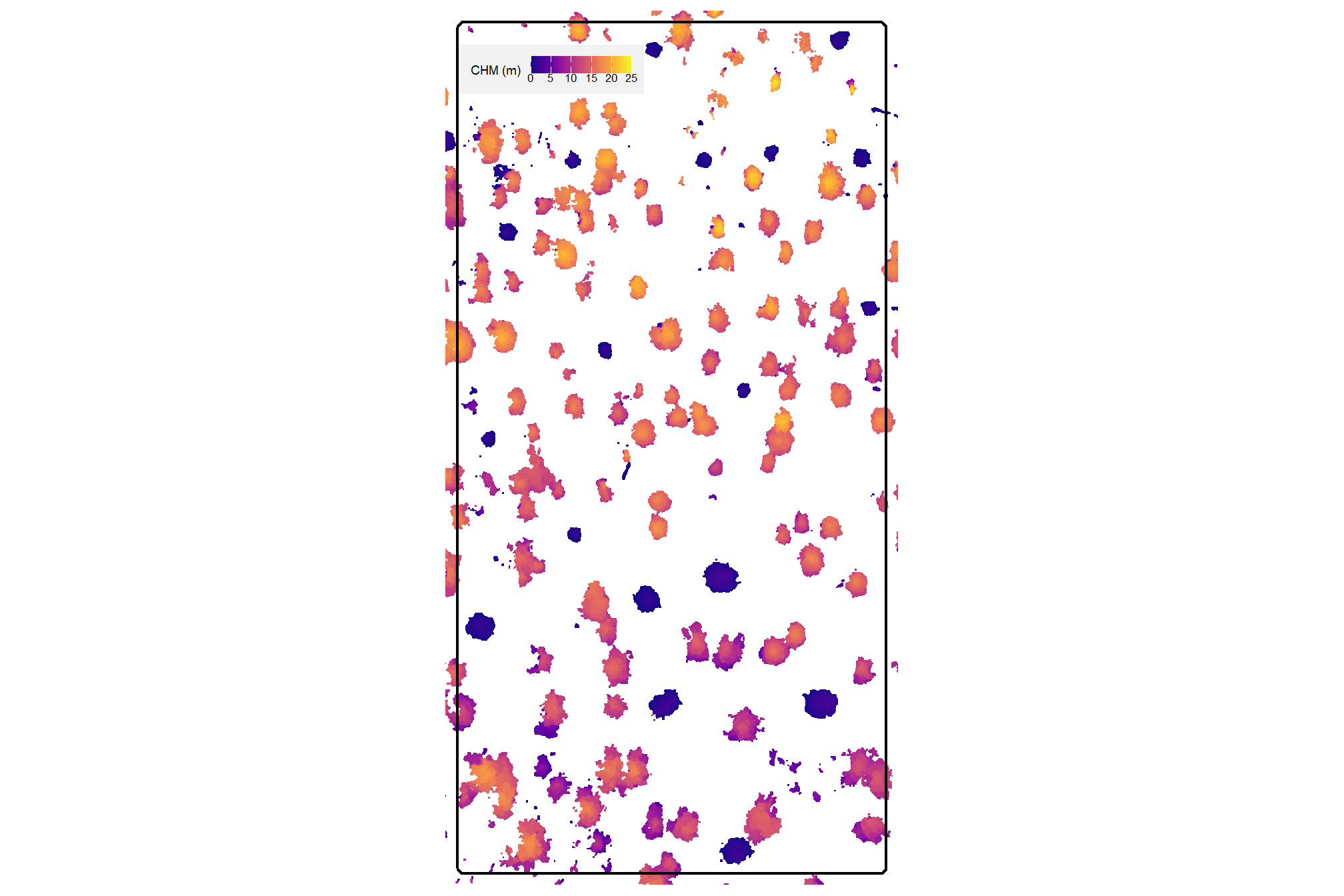
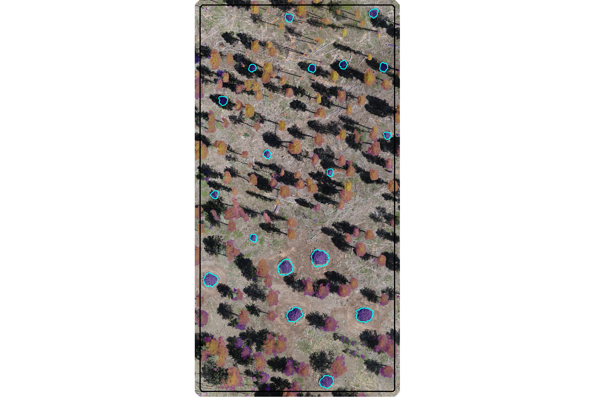
here is the RGB of the example area. can you pick out the slash piles?
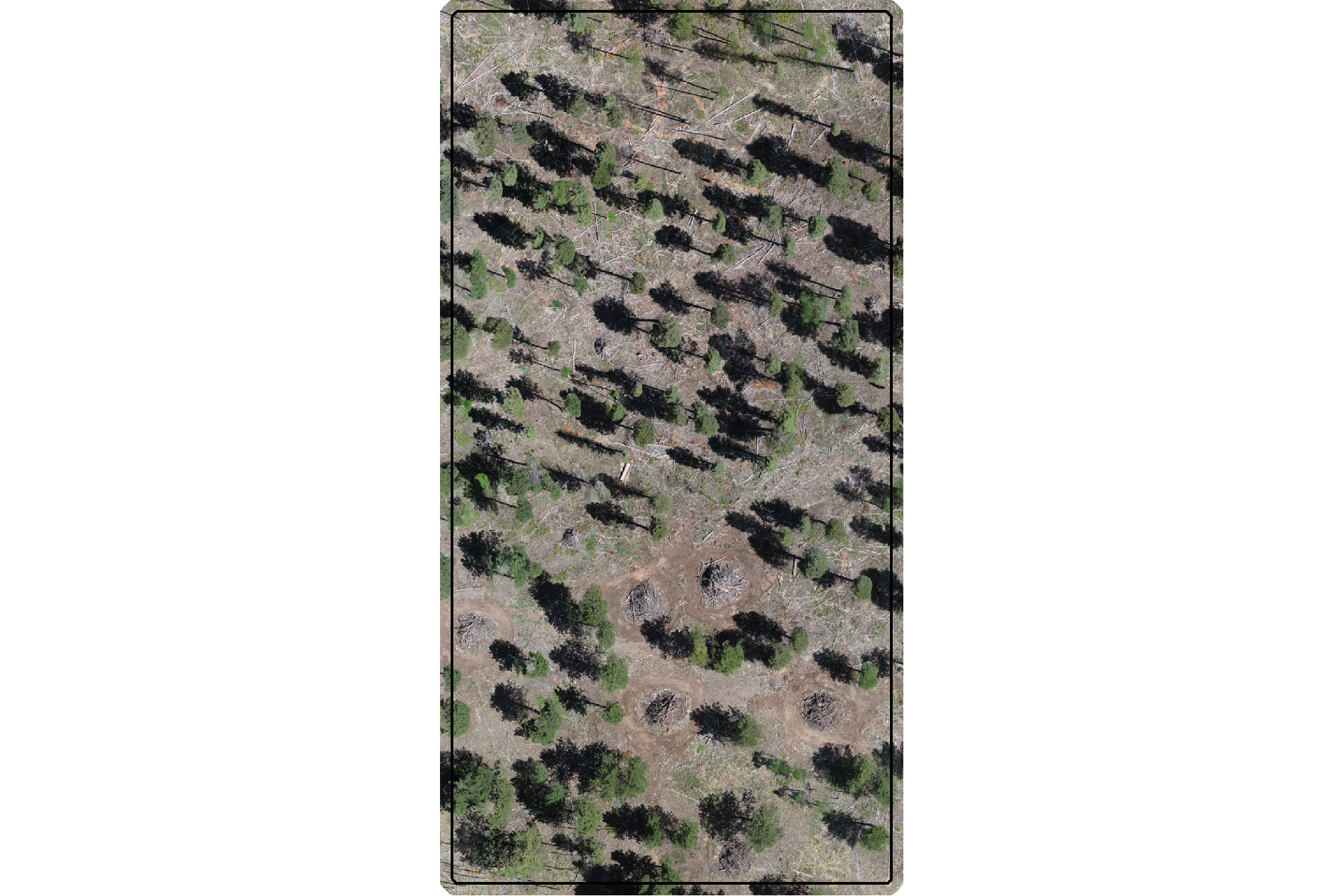
we’ll add on the ground truth piles in cyan on the RGB. how many did you find? be honest.
aoi_plt_ortho +
ggplot2::geom_sf(data = aoi_boundary, fill = NA, color = "black", lwd = 0.8) +
ggplot2::geom_sf(
data = aoi_slash_piles_polys
, fill = NA, color = "cyan", lwd = 0.95
) +
ggplot2::theme(legend.position = "none")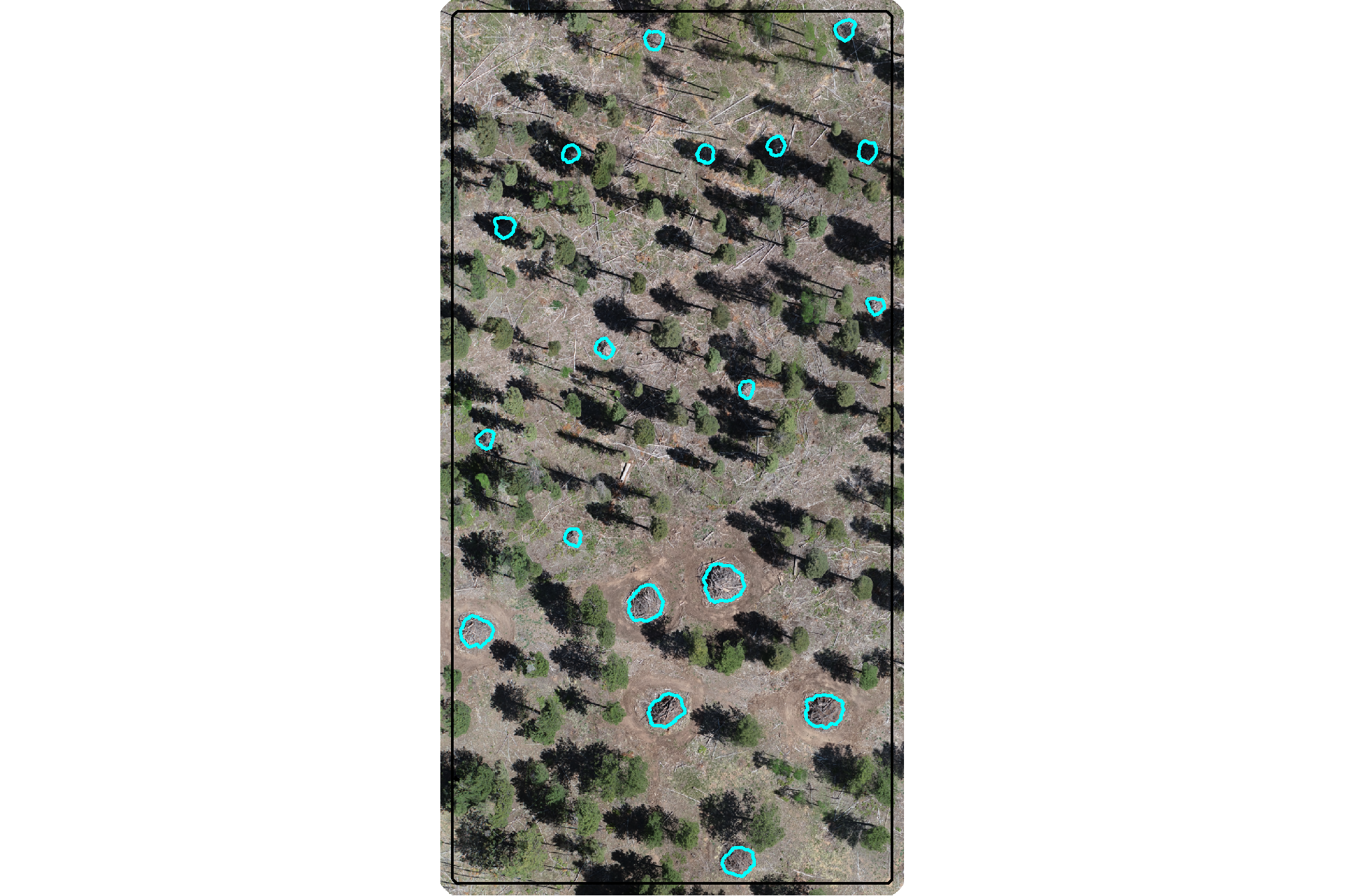
would you have done better if you had both the CHM and RGB data?
plt_aoi_chm_rgb <- function(chm) {
 aoi_plt_ortho +
    ggnewscale::new_scale_fill() +
    ggplot2::geom_tile(
      data = chm %>%
        terra::as.data.frame(xy=T) %>%
        dplyr::rename(f=3)
      , mapping = ggplot2::aes(x=x,y=y,fill=f)
      , alpha = 0.4
      , inherit.aes = F
    ) +
    ggplot2::scale_fill_viridis_c(option = "plasma") +
    ggplot2::geom_sf(data = aoi_boundary, fill = NA, color = "black", lwd = 0.8) +
    ggplot2::theme(legend.position = "none")
}
plt_aoi_chm_rgb(aoi_chm_rast) +
  ggplot2::geom_sf(
    data = aoi_slash_piles_polys
    , fill = NA, color = "cyan", lwd = 0.6
  )
4.2 Segmentation Methods
Our slash pile detection approach will align with the land manager knowledge of physical metrics of slash pile form which are commonly used in forest inventories and silvicultural prescriptions. We’ll start with input parameters like height and area thresholds.
the first step in this approach is to isolate the lower “slice” of the CHM based on a maximum height threshold defined by the upper limit of the expected slash pile height. the expected height range to search for slash piles should be based on the pile construction prescription and potentially adjusted based on a sample of field-measured values after treatment completion
we’ll set a maximum height threshold (max_ht_m) which filters the CHM to only include raster cells lower than this threshold. we’ll also set a lower height limit (min_ht_m) based on the expected slash pile height for use later in removing candidate segments that are shorter than this lower limit.
# set the max and min expected pile height
max_ht_m <- 6
min_ht_m <- 0.5
# lower CHM slice
aoi_chm_rast_slice <- terra::clamp(aoi_chm_rast, upper = max_ht_m, lower = 0, values = F)
plot the lower slice, notice how the CHM height scale has changed
plt_aoi_chm(aoi_chm_rast_slice) +
  ggplot2::geom_sf(
    data = aoi_slash_piles_polys
    , fill = NA, color = "cyan", lwd = 0.6
  )
already, it looks like the piles should be distinguishable objects from this data
our rules-based pile detection methodology will also rely on area thresholds to define a search space and filter candidate segments. like height, we’ll also set a minimum (min_area_m2) and maximum (max_area_m2) pile 2D area (in square meters) to search and filter for valid candidate objects. As with the height, these thresholds should be set based on the pile construction prescription or estimates or sample measurements from field visits.
# set the max and min expected pile area
min_area_m2 <- 1.5
# Two standard US parking spaces, typically measuring 9 feet by 18 feet,
# are roughly equivalent to 30.25 square meters. Each space is approximately 15.125 square meters.
# 15.125*3
max_area_m2 <- 50
to summarize, the size-based thresholds of our geometric, rules-based approach for detecting slash piles from CHM data are:
max_ht_m: numeric. The maximum height (in meters) a slash pile is expected to be. This value helps us focus on a specific “slice” of the data, ignoring anything taller than a typical pile.min_ht_m: numeric. The minimum height (in meters) a detected pile must reach to be considered valid.min_area_m2: numeric. The smallest 2D area (in square meters) a detected pile must cover to be considered valid.max_area_m2: numeric. The largest 2D area (in square meters) a detected pile can cover to be considered valid.
4.2.1 Overview of Methods
The two primary segmentation methods we’ll test are watershed segmentation and DBSCAN. Watershed segmentation, which we’ll implement with lidR::watershed(), is a raster-based technique that treats a CHM as a topographic surface where height values are inverted to create basins. The algorithm identifies local maxima as “seeds” and expands them until they reach a boundary or “watershed” line. This method requires a tolerance parameter (tol) which defines “the minimum height of the object…between its highest point (seed) and the point where it contacts another object…If the height is smaller than the tolerance, the object will be combined with one of its neighbors, which is the highest. Tolerance should be chosen according to the range of x.” An extent parameter (ext) is used to define the search window for object seeds.
The DBSCAN algorithm, which we’ll implement with dbscan::dbscan(), is typically a point-based clustering algorithm that groups points based on their spatial density but DBSCAN can also be applied to raster data by converting the raster cells into a 2D point set using the cell centroids. The algorithm relies on an epsilon parameter (eps), which defines the search radius around a point, and a minimum points parameter (minPts), which sets the threshold for how many neighbors must exist within that radius to form a core cluster.
Dynamically defining these parameters is critical for the usability and scalability of the method because it removes the guesswork typically required when moving between different datasets. For example, point clouds can vary in point density depending on the flight altitude or sensor, and rasters can vary in resolution. If parameters are kept static, a model tuned for a specific data structure or target object will be suboptimal for different data. We can link the segmentation algorithm parameters directly to the input data structure and the expected target object size so that the method automatically recalibrates itself.
In applying a similar, rules-based methodology for coarse woody debris detection from point cloud data, dos Santos et al. (2025) recommend setting algorithm parameters based on minimum expected object size to be detected and point density.
We developed dynamic logic to automatically bridge the gap between the expectation of the target object form (height and area thresholds) and the representation of the object in the data by using geometric ratios. For watershed segmentation, the tolerance (tol) is scaled to the height range of the target objects to ensure sensitivity to the vertical variability. The extent (ext) is calculated by converting the physical radius of the smallest expected object into a pixel count based on the raster resolution. For DBSCAN, the epsilon parameter (eps) is calculated to bridge the average gap between points (or the distance between raster cell centroids) but is capped to prevent the merging of adjacent objects. The minimum points (minPts) parameter is scaled by the ratio of the search area (eps) to the total object area, ensuring that a cluster only forms if the local point density is representative of a valid target object.
| Method | Parameter | Parameter Description | Our Dynamic Logic (R-style pseudo-code) | Logic Explanation | Why our dynamic logic works |
|---|---|---|---|---|---|
| Watershed | tol |
Minimum height difference to distinguish objects. | (max_ht_m - min_ht_m) * 0.50 |
Sets the vertical threshold at 50% of the target’s defined Z search space. | Prevents over-segmentation by requiring vertical “valleys” to be significant relative to the target’s height. |
| Watershed | ext |
Radius of the search window for detecting seeds. | max(1, round((target_radius_m * 0.5) / rast_res_m)) |
Uses 50% of the target radius as the search window, converted to pixels with a 1-pixel minimum. | Maintains a consistent physical search area regardless of raster resolution, ensuring seeds are centered on objects. |
| DBSCAN | eps |
Maximum distance to consider points as neighbors. | min(1.5 * (1/sqrt(pts_per_m2)), (target_radius_m * 0.5 * 0.5)) |
Selects the smaller of 1.5-times the point spacing or 50% of the effective radius (25% of target radius). | Ensures the point-search stays localized, effectively preventing separate objects from “bridging” together. |
| DBSCAN | minPts |
Minimum points required to form a cluster core. | round((min_area_m2 * pts_per_m2) * (eps^2 / (target_radius_m^2))) |
Scales total expected points by the ratio of the search circle area to the total target area. | Dynamically adjusts the density threshold based on the search radius, allowing for consistent detection across varying data densities. |
let’s define a function to get these parameters based on the user-defined size thresholds and the input data description
# function to get segmentation parameters
get_segmentation_params <- function(
  min_ht_m
  , max_ht_m
  , min_area_m2
  , max_area_m2
  , pts_per_m2 = NULL
  , rast_res_m = NULL
){

  # check for missing required values
  if (missing(max_ht_m) || missing(min_ht_m) ||
      missing(min_area_m2) || missing(max_area_m2)) {
    stop("all geometric constraints (max_ht_m, min_ht_m, min_area_m2, max_area_m2) must be defined.")
  }

  # geometric param validation
  if (max_ht_m <= min_ht_m) {
    stop("max_ht_m must be greater than min_ht_m.")
  }
  if (max_area_m2 <= min_area_m2) {
    stop("max_area_m2 must be greater than min_area_m2.")
  }
  if (min_ht_m < 0 || min_area_m2 < 0) {
    stop("height and area constraints must be positive values.")
  }

  # data structure validation and calculation
  if (is.null(pts_per_m2) && is.null(rast_res_m)) {
    stop("must provide either 'pts_per_m2' (pts/m2) or 'rast_res_m' (m/pixel).")
  }

  # calculate and validate data str values
  if (is.null(pts_per_m2)) {
    if (rast_res_m <= 0) stop("rast_res_m must be a positive value.")
    pts_per_m2 <- 1 / (rast_res_m^2)
  }
  if (is.null(rast_res_m)) {
    if (pts_per_m2 <= 0) stop("pts_per_m2 must be a positive value.")
    rast_res_m <- 1 / sqrt(pts_per_m2)
  }
  ################################################
  # lidR::watershed / EBImage::watershed
  ################################################
  # lidR::watershed `tol`
  # set based on the height range
  height_range <- max_ht_m - min_ht_m
  # scale it to increase the sensitivity to distinguish smaller objects
  tol_val <- height_range * 0.5

  # lidR::watershed `ext`
  # use ~half~ quarter the radius of the minimum object to increase sensitivity
  # this helps prevent merging nearby objects (under-segmentation)
  target_radius_m <- sqrt(min_area_m2 / pi)
  effective_radius_m <- target_radius_m * 0.25
  ext_val <- max(1, round(effective_radius_m / rast_res_m))

  ################################################
  # dbscan::dbscan
  ################################################
  # dbscan::dbscan `eps` (epsilon)
  # [dos Santos et al. (2025)](https://doi.org/10.3390/rs17040651) recommended to set this value based:
    # "on the minimum cluster size to be detected and point density"

  # start by scaling based on point spacing (1.5x average distance between points).
  spacing <- 1 / sqrt(pts_per_m2)
  connectivity_eps <- 1.5 * spacing
  # eps should not exceed 25% of the minimum object radius to avoid merging separate objects into one cluster.
  max_allowable_eps <- target_radius_m * 0.25
  # cap eps by the object size constraint
  # as long as the quarter-radius of your min_area_m2 is
  # greater than the pixel diagonal (1.5*spacing), the algorithm will function well and stay above the point density limit
  eps_val <- min(connectivity_eps, max_allowable_eps)
  ### option 1b:
  # eps_val <- max(connectivity_eps, max_allowable_eps) # to ensure it doesn't go below data resolutoin
  ### option 2:
  # eps_val <- min(2 / sqrt(pts_per_m2), 0.5 * sqrt(min_area_m2 / pi))
  # $epsilon = \min\!\left(\frac{2}{\sqrt{\text{pt\_dens}}},\;\frac{1}{2}\sqrt{\frac{\text{min\_area}}{\pi}}\right)$
  ### option 3:
  # eps_val <- 1 / sqrt(pi * pts_per_m2)
  # $epsilon = 1 / sqrt(pts_per_m2)$

  # dbscan::dbscan `minPts`
  # based on expected points within the epsilon neighborhood area

  # get expected number of points in an object of min_area_m2
  expected_pts_in_min_object <- min_area_m2 * pts_per_m2

  # ensure a core point is surrounded by a density of points based on min_area_m2 size at point density
  # scale the total expected points of the minimum object
    # by the ratio of the epsilon-neighborhood area to the total minimum object area
    # to ensure a core point meets the expected density of the target object
  pts_ratio_calc <- expected_pts_in_min_object * (eps_val^2 / target_radius_m^2)
  min_pts_val <- max(
    5 # don't go any lower than the dbscan::dbscan() default
    , round(pts_ratio_calc)
  )

  # return
  return(list(
    data_summary = list(pts_per_m2 = pts_per_m2, rast_res_m = rast_res_m),
    watershed = list(tol = tol_val, ext = ext_val),
    dbscan = list(eps = eps_val, minPts = min_pts_val)
  ))
}
let’s test our get_segmentation_params() function using the size threshold parameters we defined above: max_ht_m, min_ht_m, min_area_m2, max_area_m2 and we can get the raster resolution directly from our input CHM
# get_segmentation_params
get_segmentation_params_ans <- get_segmentation_params(
    max_ht_m = max_ht_m
    , min_ht_m = min_ht_m
    , min_area_m2 = min_area_m2
    , max_area_m2 = max_area_m2
    # , pts_per_m2 = NULL
    , rast_res_m = terra::res(aoi_chm_rast_slice)[1]
  )
# huh?
dplyr::glimpse(get_segmentation_params_ans)
## List of 3
## $ data_summary:List of 2
## ..$ pts_per_m2: num 100
## ..$ rast_res_m: num 0.1
## $ watershed :List of 2
## ..$ tol: num 2.75
## ..$ ext: num 2
## $ dbscan :List of 2
## ..$ eps : num 0.15
## ..$ minPts: num 7we can see how these parameters change if the CHM resolution changes
get_segmentation_params(
    max_ht_m = max_ht_m
    , min_ht_m = min_ht_m
    , min_area_m2 = min_area_m2
    , max_area_m2 = max_area_m2
    # , pts_per_m2 = NULL
    , rast_res_m = 0.5
  ) %>%
  dplyr::glimpse()
## List of 3
## $ data_summary:List of 2
## ..$ pts_per_m2: num 4
## ..$ rast_res_m: num 0.5
## $ watershed :List of 2
## ..$ tol: num 2.75
## ..$ ext: num 1
## $ dbscan :List of 2
## ..$ eps : num 0.173
## ..$ minPts: num 5and we can see how these parameters change using our CHM data but change the expected minimum pile 2D area
get_segmentation_params(
    max_ht_m = max_ht_m
    , min_ht_m = min_ht_m
    , min_area_m2 = 22
    , max_area_m2 = max_area_m2
    # , pts_per_m2 = NULL
    , rast_res_m = terra::res(aoi_chm_rast_slice)[1]
  ) %>%
  dplyr::glimpse()
## List of 3
## $ data_summary:List of 2
## ..$ pts_per_m2: num 100
## ..$ rast_res_m: num 0.1
## $ watershed :List of 2
## ..$ tol: num 2.75
## ..$ ext: num 7
## $ dbscan :List of 2
## ..$ eps : num 0.15
## ..$ minPts: num 7the table summarizes how our rules-based approach creates dynamic parameters for use in watershed and DBSCAN segmentation. The height parameters manage vertical noise, the area parameters manage horizontal separation, and the data resolution parameters ensure the math stays consistent regardless of data density (raster resolution or point cloud point density).
| Dynamic Parameter | Impact of Height (max_ht_m / min_ht_m) |
Impact of Target Area (min_area_m2) |
Impact of Data Structure (rast_res_m / pts_per_m2) |
|---|---|---|---|
Watershed tol |
Direct Driver: Sets the vertical threshold at 50% of the target’s defined Z search space. | None: Vertical tolerance is independent of horizontal footprint. | None: Vertical sensitivity is independent of horizontal resolution. |
Watershed ext |
None: Horizontal search window is independent of vertical range. | Geometric Baseline: Defines the physical radius used to scale the search window at a 1:2 ratio. | Spatial Divider: Converts the physical radius into a pixel count using rast_res_m with a 1-pixel minimum. |
DBSCAN eps |
None: Point-to-point connectivity is independent of height. | Physical Cap: Limits search distance to 50% of the effective radius (25% of target radius) to ensure separation. | Connectivity Anchor: Sets the search radius at 1.5-times the spacing derived from pts_per_m2 to maintain tight clusters. |
DBSCAN minPts |
None: Required point mass is independent of vertical range. | Total Mass Baseline: Defines the total expected points for the smallest valid target. | Density Multiplier: Calculates the local point count requirement relative to the pts_per_m2 value. |
sim_df_temp <-
  tidyr::crossing(
    rast_res_m = seq(0.1, 1.3, by = 0.1)
    , min_area_m2 = seq(1, 50, length.out = 33)
  ) %>%
  dplyr::mutate(
    # Call the pre-defined function directly to ensure logic alignment
    params = purrr::map2(
      rast_res_m, min_area_m2, ~ get_segmentation_params(
        max_ht_m = max_ht_m
        , min_ht_m = min_ht_m
        , min_area_m2 = .y
        , max_area_m2 = .y * 5
        , rast_res_m = .x
      )
    )

    # Extract values into individual columns for plotting
    , ext = purrr::map_dbl(params, ~ .x$watershed$ext)
    , eps = purrr::map_dbl(params, ~ .x$dbscan$eps)
    , min_pts = purrr::map_dbl(params, ~ .x$dbscan$minPts)
  )
  # # Pivot to long format for faceted plotting
  # tidyr::pivot_longer(
  #   cols = c(ext, eps, min_pts),
  #   names_to = "parameter",
  #   values_to = "value"
  # )
# sim_df_temp %>% dplyr::glimpse()

# plot
p1_temp <-
  ggplot2::ggplot(sim_df_temp, ggplot2::aes(x = rast_res_m, y = min_area_m2, fill = ext)) +
  ggplot2::geom_tile(col = "gray") +
  ggplot2::scale_fill_viridis_c(option = "magma") +
  ggplot2::scale_x_continuous(expand = c(0, 0), breaks = scales::breaks_extended(n=10)) +
  ggplot2::scale_y_continuous(expand = c(0, 0), breaks = scales::breaks_extended(n=10)) +
  ggplot2::labs(title = "Watershed: `ext` (pixels)", fill = "pixels") +
  ggplot2::theme_light() +
  ggplot2::theme(legend.position = "bottom", plot.title = ggplot2::element_text(size = 9))

p2_temp <-
  ggplot2::ggplot(sim_df_temp, ggplot2::aes(x = rast_res_m, y = min_area_m2, fill = eps)) +
  ggplot2::geom_tile(col = "gray") +
  ggplot2::scale_fill_viridis_c(option = "magma") +
  ggplot2::scale_x_continuous(expand = c(0, 0), breaks = scales::breaks_extended(n=10)) +
  ggplot2::scale_y_continuous(expand = c(0, 0), breaks = scales::breaks_extended(n=10)) +
  ggplot2::labs(title = "DBSCAN: `eps` (meters)", fill = "meters") +
  ggplot2::theme_light() +
  ggplot2::theme(legend.position = "bottom", plot.title = ggplot2::element_text(size = 9))

p3_temp <-
  ggplot2::ggplot(sim_df_temp, ggplot2::aes(x = rast_res_m, y = min_area_m2, fill = min_pts)) +
  ggplot2::geom_tile(col = "gray") +
  ggplot2::scale_fill_viridis_c(option = "magma") +
  ggplot2::scale_x_continuous(expand = c(0, 0), breaks = scales::breaks_extended(n=10)) +
  ggplot2::scale_y_continuous(expand = c(0, 0), breaks = scales::breaks_extended(n=10)) +
  ggplot2::labs(title = "DBSCAN: `minPts` (count)", fill = "count") +
  ggplot2::theme_light() +
  ggplot2::theme(legend.position = "bottom", plot.title = ggplot2::element_text(size = 9))

# 5. Combine using patchwork
(p1_temp + p2_temp + p3_temp) +
  patchwork::plot_annotation(
    title = "Dynamic Watershed and DBSCAN Parameter Definition"
    , subtitle = "across raster resolution and minimum target area gradients"
    , theme = ggplot2::theme(plot.title = ggplot2::element_text(size = 10),plot.subtitle = ggplot2::element_text(size = 8))
  ) +
  patchwork::plot_layout(ncol = 3)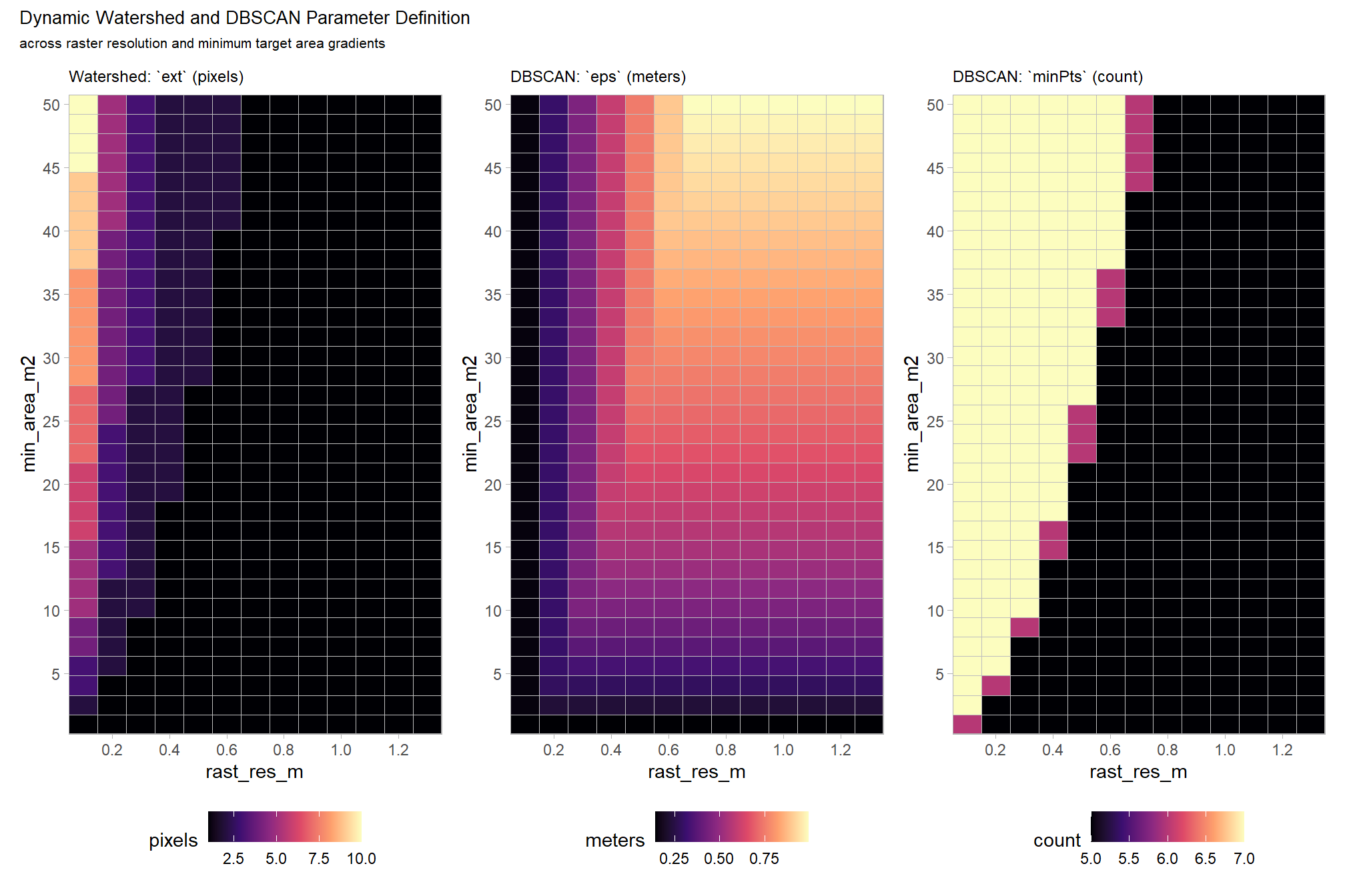
4.2.2 Watershed Segmentation Demonstration
let’s go through the watershed segmentation process using lidR::watershed() which is based on the bioconductor package EBIimage
# ?EBImage::watershed
watershed_segs <- lidR::watershed(
    chm = aoi_chm_rast_slice
    # th_tree = Threshold below which a pixel cannot be a tree. Default is 2.
    , th_tree = 0.01
    # tol = minimum height of the object in the units of image intensity between its highest point (seed)
      # and the point where it contacts another object (checked for every contact pixel).
      # If the height is smaller than the tolerance, the object will be combined with one of its neighbors, which is the highest.
      # Tolerance should be chosen according to the range of x
    , tol = get_segmentation_params_ans$watershed$tol # max_ht_m-min_ht_m
    # ext = Radius of the neighborhood in pixels for the detection of neighboring objects.
      # Higher value smoothes out small objects.
    , ext = get_segmentation_params_ans$watershed$ext # 1
  )()
the result is a raster with cells segmented and given a unique identifier
## class       : SpatRaster
## size        : 1483, 768, 1  (nrow, ncol, nlyr)
## resolution  : 0.1, 0.1  (x, y)
## extent      : 499310.2, 499387, 4317710, 4317858  (xmin, xmax, ymin, ymax)
## coord. ref. : WGS 84 / UTM zone 13N (EPSG:32613)
## source(s)   : memory
## varname     : aoi_chm_rast
## name        : focal_mean
## min value   :          1
## max value   :        214
each value should be a unique “segment” which we can refine based on rules of expected size and shape of piles
##    layer value count
## 1      1   181    16
## 2      1    19    26
## 3      1   131    18
## 4      1   171     9
## 5      1    99    21
## 6      1    21    71
## 7      1   180    45
## 8      1   106    13
## 9      1    43   443
## 10     1    18     2
where the “value” is the segment identifier and the count is the number of raster cells assigned to that segment
how many predicted segments are there?
## [1] 214let’s plot the raster return from the watershed segmentation
watershed_segs %>%
  terra::as.factor() %>%
  terra::plot(
    col = c(
      viridis::turbo(n = terra::minmax(watershed_segs)[2])
      # , viridis::viridis(n = floor(terra::minmax(watershed_segs)[2]/3))
      # , viridis::cividis(n = floor(terra::minmax(watershed_segs)[2]/3))
    ) %>% sample()
    , legend = F
    , axes = F
  )
plot the watershed candidate segments (magenta) and the actual piles (cyan) on the RGB
aoi_plt_ortho +
  ggplot2::geom_sf(data = aoi_boundary, fill = NA, color = "black", lwd = 0.8) +
  ggplot2::geom_sf(
    data = aoi_slash_piles_polys
    , fill = NA, color = "cyan", lwd = 0.9
  ) +
  ggplot2::geom_sf(
    data = watershed_segs %>%
      terra::as.polygons(round = F, aggregate = T, values = T, extent = F, na.rm = T) %>%
      setNames("pred_id") %>%
      sf::st_as_sf() %>%
      sf::st_simplify() %>%
      sf::st_make_valid() %>%
      dplyr::filter(sf::st_is_valid(.))
    , fill = NA, color = "magenta", lwd = 0.6
  ) +
  ggplot2::theme(legend.position = "none")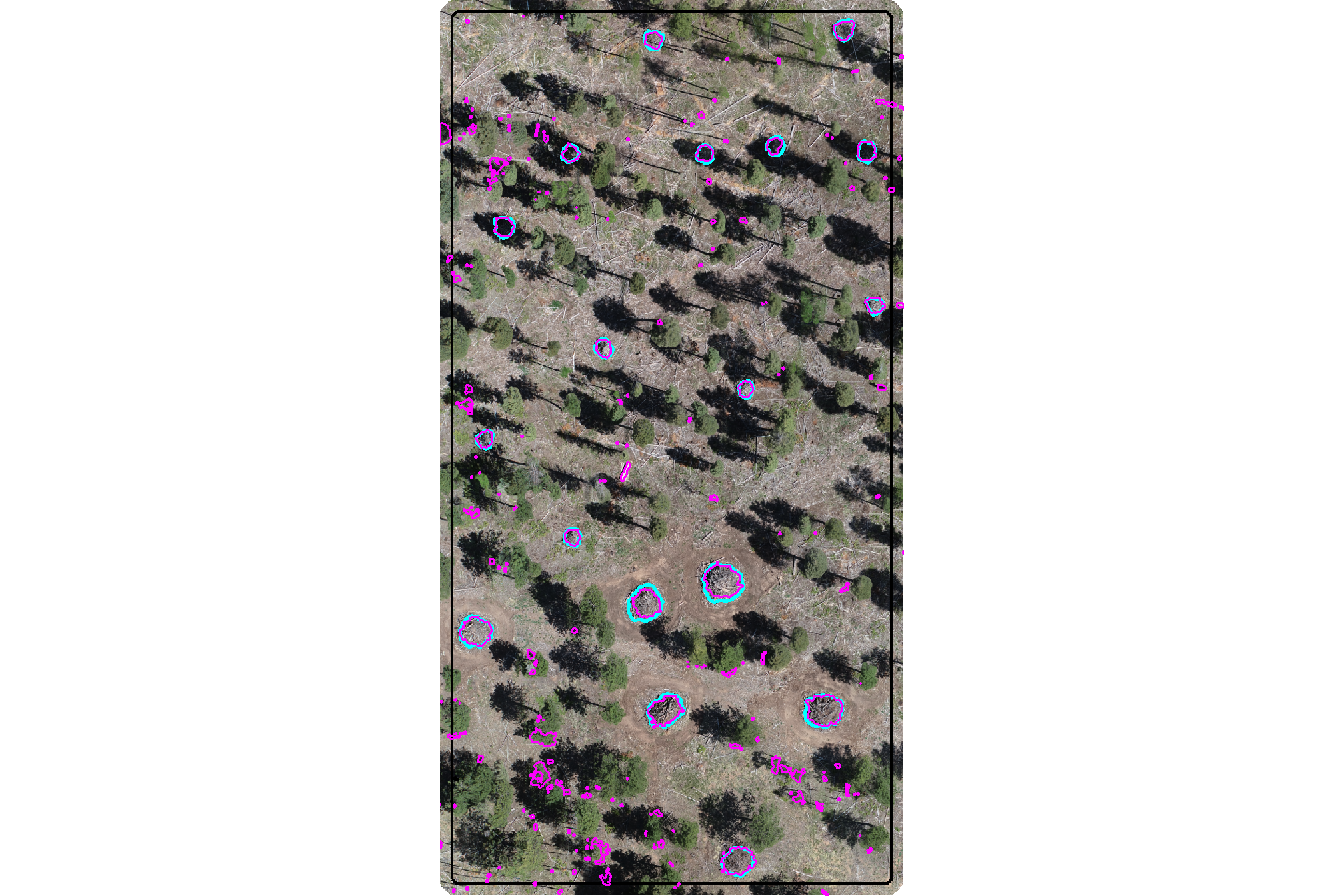
plot the watershed candidate segments (magenta) and the actual piles (cyan) on the CHM
plt_aoi_chm(aoi_chm_rast_slice) +
  ggplot2::geom_sf(
    data = aoi_slash_piles_polys
    , fill = NA, color = "cyan", lwd = 0.6
  ) +
  ggplot2::geom_sf(
    data = watershed_segs %>%
      terra::as.polygons(round = F, aggregate = T, values = T, extent = F, na.rm = T) %>%
      setNames("pred_id") %>%
      sf::st_as_sf() %>%
      sf::st_simplify() %>%
      sf::st_make_valid() %>%
      dplyr::filter(sf::st_is_valid(.))
    , fill = NA, color = "magenta", lwd = 0.6
  )
nice…we are getting close.
4.2.3 DBSCAN Segmentation Demonstration
let’s go through the DBSCAN segmentation process using dbscan::dbscan() which uses a kd-tree for efficient processing. As an aside, the RANN package enables KD-tree searching/processing using the X and Y coordinates of the entire point cloud to build the tree which is a super-fast way to find the x number of near neighbors for each point in an input dataset (see RANN::nn2()).
because the DBSCAN process is a point-based clustering algorithm that groups points based on their spatial density we need to convert the raster cells into a 2D point set using the cell centroids first
## XY df
xy_df_temp <-
  aoi_chm_rast_slice %>%
  # na.rm = T ensures we only process cells with CHM data
  terra::as.data.frame(xy = T, na.rm = T) %>%
  dplyr::rename(
    X=x,Y=y
    , f=3
  ) %>%
  dplyr::select(X,Y)
# huh?
xy_df_temp %>% dplyr::glimpse()
## Rows: 27,616
## Columns: 2
## $ X <dbl> 499324.0, 499324.0, 499324.0, 499330.2, 499330.4, 499330.5, 499324.0…
## $ Y <dbl> 4317856, 4317856, 4317856, 4317856, 4317856, 4317856, 4317856, 43178…# ggplot2::ggplot(data = xy_df_temp, mapping = ggplot2::aes(x=X,y=Y)) + ggplot2::geom_point(shape=".")now, we can apply the dbscan::dbscan() function using the parameters we identified using our dynamic process defined in get_segmentation_params()
# get_segmentation_params_ans %>% dplyr::glimpse()
# ?dbscan::dbscan
dbscan_ans_temp <- dbscan::dbscan(
  x = xy_df_temp
  # eps primarily controls the spatial extent of a cluster,
  # as it defines how far points can be from each other to be considered part of the same dense region.
  , eps = get_segmentation_params_ans$dbscan$eps
  # minPts primarily controls the minimum density of a cluster,
  # as it dictates how many points must be packed together within that eps radius.
  , minPts = get_segmentation_params_ans$dbscan$minPts
)
# huh?
dbscan_ans_temp %>% str()
## List of 5
## $ cluster : int [1:27616] 0 0 0 1 1 1 0 1 1 1 ...
## $ eps : num 0.15
## $ minPts : num 7
## $ metric : chr "euclidean"
## $ borderPoints: logi TRUE
## - attr(*, "class")= chr [1:2] "dbscan_fast" "dbscan"the result is a vector with a cluster identifier for each point we provided to the algorithm
## [1] TRUEadd the cluster identifier to the XY point data
# add the cluster to the data
xy_df_temp$cluster <- dbscan_ans_temp$cluster
# what?
xy_df_temp %>%
  dplyr::count(cluster) %>%
  dplyr::arrange(desc(n)) %>%
  head()
## cluster n
## 1 102 2398
## 2 118 2303
## 3 119 1821
## 4 181 1785
## 5 108 1754
## 6 107 1539to maintain processing consistency with the watershed result, we’ll rasterize the XY data back to the original CHM grid. this will result in a raster with cells segmented and given the unique identifier.
Note: the cells/segments classified as noise from the dbscan::dbscan() algorithm are marked with a cluster identifier as “0”…we’ll remove these prior to rasterizing
# fill the rast with the cluster values
dbscan_segs <- terra::rasterize(
  x = xy_df_temp %>%
    dplyr::filter(cluster!=0) %>%
    sf::st_as_sf(coords = c("X", "Y"), crs = terra::crs(aoi_chm_rast_slice), remove = F) %>%
    dplyr::ungroup() %>%
    dplyr::select(cluster) %>%
    terra::vect()
  , y = aoi_chm_rast_slice
  , field = "cluster"
)
the result is a raster with cells segmented and given a unique identifier
## class       : SpatRaster
## size        : 1483, 768, 1  (nrow, ncol, nlyr)
## resolution  : 0.1, 0.1  (x, y)
## extent      : 499310.2, 499387, 4317710, 4317858  (xmin, xmax, ymin, ymax)
## coord. ref. : WGS 84 / UTM zone 13N (EPSG:32613)
## source(s)   : memory
## varname     : aoi_chm_rast
## name        : last
## min value   :    1
## max value   :  200
each value should be a unique “segment” which we can refine based on rules of expected size and shape of piles
##   layer value count
## 1     1   102  2398
## 2     1   118  2303
## 3     1   119  1821
## 4     1   181  1785
## 5     1   108  1754
## 6     1   107  1539
where the “value” is the segment identifier and the count is the number of raster cells assigned to that segment (compare to the count of the segmented points above ;)
how many predicted segments are there?
## [1] 200let’s plot the raster of the dbscan segmentation
dbscan_segs %>%
  terra::as.factor() %>%
  terra::plot(
    col = c(
      viridis::turbo(n = terra::minmax(dbscan_segs)[2])
    ) %>% sample()
    , legend = F
    , axes = F
  )
plot the watershed candidate segments (magenta) and the actual piles (cyan) on the RGB
aoi_plt_ortho +
  ggplot2::geom_sf(data = aoi_boundary, fill = NA, color = "black", lwd = 0.8) +
  ggplot2::geom_sf(
    data = aoi_slash_piles_polys
    , fill = NA, color = "cyan", lwd = 0.9
  ) +
  ggplot2::geom_sf(
    data = dbscan_segs %>%
      terra::as.polygons(round = F, aggregate = T, values = T, extent = F, na.rm = T) %>%
      setNames("pred_id") %>%
      sf::st_as_sf() %>%
      sf::st_simplify() %>%
      sf::st_make_valid() %>%
      dplyr::filter(sf::st_is_valid(.))
    , fill = NA, color = "magenta", lwd = 0.6
  ) +
  ggplot2::theme(legend.position = "none")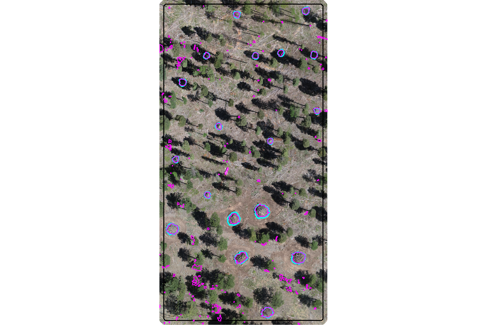
plot the watershed candidate segments (magenta) and the actual piles (cyan) on the CHM
plt_aoi_chm(aoi_chm_rast_slice) +
  ggplot2::geom_sf(
    data = aoi_slash_piles_polys
    , fill = NA, color = "cyan", lwd = 0.6
  ) +
  ggplot2::geom_sf(
    data = dbscan_segs %>%
      terra::as.polygons(round = F, aggregate = T, values = T, extent = F, na.rm = T) %>%
      setNames("pred_id") %>%
      sf::st_as_sf() %>%
      sf::st_simplify() %>%
      sf::st_make_valid() %>%
      dplyr::filter(sf::st_is_valid(.))
    , fill = NA, color = "magenta", lwd = 0.6
  )
nice…we are getting close.
4.2.4 Comparison of Candidate Segments
we’ll start by converting the candidate segments to polygons
# watershed_segs
watershed_segs_poly <-
  watershed_segs %>%
  terra::as.polygons(round = F, aggregate = T, values = T, extent = F, na.rm = T) %>%
  setNames("pred_id") %>%
  sf::st_as_sf() %>%
  sf::st_simplify() %>%
  sf::st_make_valid() %>%
  dplyr::filter(sf::st_is_valid(.))
# dbscan_segs
dbscan_segs_poly <-
  dbscan_segs %>%
  terra::as.polygons(round = F, aggregate = T, values = T, extent = F, na.rm = T) %>%
  setNames("pred_id") %>%
  sf::st_as_sf() %>%
  sf::st_simplify() %>%
  sf::st_make_valid() %>%
  dplyr::filter(sf::st_is_valid(.))
count the number of unique candidate segments from each method and summarize the area covered by all segments
dplyr::tibble(
    method = c("watershed", "DBSCAN")
    , segments = c(
      terra::freq(watershed_segs) %>% nrow()
      , terra::freq(dbscan_segs) %>% nrow()
    )
    , area = c(
      watershed_segs_poly %>% sf::st_union() %>% sf::st_area() %>% as.numeric()
      , dbscan_segs_poly %>% sf::st_union() %>% sf::st_area() %>% as.numeric()
    )
  ) %>%
  dplyr::mutate(
    segments = scales::comma(segments,accuracy=1)
    , area = scales::comma(area,accuracy=0.01)
  ) %>%
  kableExtra::kbl(
    caption = "Demonstration area candidate segments by method"
    , col.names = c(
      "method", "candidate segments", "area (m<sup>2</sup>)"
    )
    , escape = F
  ) %>%
kableExtra::kable_styling()| method | candidate segments | area (m2) |
|---|---|---|
| watershed | 214 | 276.16 |
| DBSCAN | 200 | 274.16 |
notice the dbscan segments cover a smaller area because noise points are identified and removed as part of the algorithm. in the next stage of our method, we’ll include additional noise removal applied to both methodologies. In fact, all processing will be the same from here forward for both segementation methodologies.
4.2.5 Segmentation Function
let’s make a function to perform either the watershed (lidR::watershed()) or DBSCAN (dbscan::dbscan()) segmentation given an input CHM raster, target height range, and target area range. the output will include a raster and sf polygons of the candidate segments
############################################################################
# DBSCAN function
# to align input of raster and output of raster as in lidR::watershed()
# this enables dbscan, typically a point-based method,
# to be implemented with raster input data by using cell centroids
############################################################################
get_segs_dbscan <- function(
  chm_rast
  , eps
  , minPts
) {
  ########################
  # check raster
  ########################
  # convert to SpatRaster if input is from 'raster' package
  if(
    inherits(chm_rast, "RasterStack")
    || inherits(chm_rast, "RasterBrick")
  ){
    chm_rast <- terra::rast(chm_rast)
  }else if(!inherits(chm_rast, "SpatRaster")){
    stop("Input 'chm_rast' must be a SpatRaster from the `terra` package")
  }
  # first layer only
  if(terra::nlyr(chm_rast)>1){warning("...only using first layer of raster stack for segmentation")}
  chm_rast <- chm_rast %>% terra::subset(subset = 1)
  # na check
  if(
    as.numeric(terra::global(chm_rast, fun = "isNA")) == terra::ncell(chm_rast)
    # || as.numeric(terra::global(chm_rast, fun = "isNA")) >= round(terra::ncell(chm_rast)*0.98)
  ){
    stop("Input 'chm_rast' has all missing values")
  }

  ########################
  # get cell centroids as points
  ########################
  ## XY df
  xy_df_temp <-
    chm_rast %>%
    # na.rm = T ensures we only process cells with CHM data
    terra::as.data.frame(xy = T, na.rm = T) %>%
    dplyr::rename(
      X=x,Y=y
      , f=3
    ) %>%
    dplyr::select(X,Y)
  # huh?
  # xy_df_temp %>% dplyr::glimpse()
  # ggplot2::ggplot(data = xy_df_temp, mapping = ggplot2::aes(x=X,y=Y)) + ggplot2::geom_point(shape=".")

  if(nrow(xy_df_temp)==0){stop("Input 'chm_rast' has all missing values")}

  ########################
  # dbscan::dbscan()
  ########################
  # ?dbscan::dbscan
  dbscan_ans_temp <- dbscan::dbscan(
    x = xy_df_temp
    # eps primarily controls the spatial extent of a cluster,
    # as it defines how far points can be from each other to be considered part of the same dense region.
    , eps = eps
    # minPts primarily controls the minimum density of a cluster,
    # as it dictates how many points must be packed together within that eps radius.
    , minPts = minPts
  )
  # ensure the result is a vector with a `cluster` identifier for each point we provided to the algorithm
  if(
    !identical(
      length(dbscan_ans_temp$cluster)
      , nrow(xy_df_temp)
    )
  ){
    stop("dbscan::dbscan() length mismatch")
  }
  # add the cluster identifier to the XY point data
  xy_df_temp$cluster <- dbscan_ans_temp$cluster
  # # what?
  # xy_df_temp %>%
  #   dplyr::count(cluster) %>%
  #   dplyr::arrange(desc(n)) %>%
  #   head()

  if(
    nrow( xy_df_temp %>% dplyr::filter(cluster!=0) ) == 0
  ){
    stop("dbscan::dbscan() result is all noise based on 'eps' and 'minPts'. try adjusting these parameters.")
  }

  ########################
  # back to raster data
  ########################
  # to maintain processing consistency with the watershed result
    # we'll rasterize the XY data back to the original CHM grid
    # this will result in a raster with cells segmented and given the unique identifier.
    # *Note*: the cells/segments classified as noise from the `dbscan::dbscan()`
    # algorithm are marked with a cluster identifier as "0"...we'll remove these prior to rasterizing
  # fill the rast with the cluster values
  dbscan_segs <- terra::rasterize(
    x = xy_df_temp %>%
      dplyr::filter(cluster!=0) %>%
      sf::st_as_sf(coords = c("X", "Y"), crs = terra::crs(chm_rast), remove = F) %>%
      dplyr::ungroup() %>%
      dplyr::select(cluster) %>%
      terra::vect()
    , y = chm_rast
    , field = "cluster"
  ) %>%
  setNames("cluster")
  # the result is a raster with cells segmented and given a unique identifier
  # this is a raster
  # dbscan_segs
  return(dbscan_segs)
}
# # ?dbscan::dbscan
# get_segs_dbscan(aoi_chm_rast_slice, minPts = 5, eps = 1) %>%
#   terra::as.factor() %>%
#   terra::plot(legend = F, col = grDevices::rainbow(n=111) %>% sample() )

############################################################################
############################################################################
############################################################################
# handle !inMemory input rasters
# !terra::inMemory(rast) means that the raster is not loaded into RAM and is (potentially) too large to do so
# `lidR::watershed()` "Cannot segment the trees from a raster stored on disk. Use segment_trees() or load the raster in memory"
# make a workflow to:
# 1) check terra::inMemory():
#   - if already loaded, run lidR::watershed() as-is to bypass tiling step and return watershed segments
# 2) if !inMemory, use terra::makeTiles() to make raster chunks with buffers that overlap neighboring tiles
# 3) each tile is processed individually using lidR::watershed() with segments converted to polygons
# 4) separate segments into "hold out" (entirely within the core, non-buffer) and "boundary" (any overlap with buffer) groups
# 5) for boundary segments: any segments that overlap are compared with only the largest segment kept (smaller, overlapping discarded) using terra::pairs()
# 6) final set of segments combines the hold outs with the processed boundary segments and return rasterized segments to match lidR::watershed() output
############################################################################
############################################################################

############################################################################
# intermediate function to set tile size based on raster size and mem available
############################################################################
get_tile_size <- function(
  rast
  , memory_risk = 0.35
  # low risk (0.01 – 0.20): creates more tiles but is unlikely to crash R
  # med risk (0.2-0.5): reserves ~95% of free RAM for the remaining calculations
  # high risk (0.5-0.7): fewer tiles but more likely to crash R
  # dangerous (>0.7): very likely to crash R
){
  # is file path or current terra obj?
  if(inherits(rast, "character") && stringr::str_ends(rast,"\\.tif$|\\.tiff$")) {
    if(!file.exists(rast)) {
      stop("the provided file path does not exist.")
    }
    my_rast <- terra::rast(rast)
  }else if(inherits(rast, "SpatRaster")) {
    my_rast <- rast
  }else{
    stop("'rast' must be a .tif|.tiff file path string or a SpatRaster object.")
  }

  # terra::free_RAM() returns the amount of RAM that is available in Bytes
  # ?terra::free_RAM
  free_ram <- terra::free_RAM()

  # logic: (available ram * risk tolerance) / bytes per double-precision pixel (8)
  # higher risk tolerance allows more pixels per tile, reducing total tile count
  max_pixels <- (free_ram * memory_risk) / 8

  # calculate tile dimension
  # sqrt to define side length in pixels
  optimal_side <- floor(sqrt(max_pixels))

  # specify the number of rows and columns for each tile (1 or 2 numbers if the number of rows and columns is not the same)
  # ?terra::makeTiles 'y' argument
  # limit the tile size at the actual raster dimensions
  optimal_side <- min(optimal_side, terra::nrow(my_rast), terra::ncol(my_rast))

  # total tile count based on rast size
  n_tiles_cols <- ceiling(terra::ncol(my_rast) / optimal_side)
  n_tiles_rows <- ceiling(terra::nrow(my_rast) / optimal_side)

  # message(paste0("current free ram: ", round(free_ram / 1e9, 2), " gb"))
  # message(paste0("memory risk: ", memory_risk))
  # message(paste0("my tile size: ", optimal_side, " pixels"))

  return(list(
    # tile_size = number of rows and columns for each zone in terra::makeTiles 'y' argument
    tile_size = optimal_side
    , total_tiles = n_tiles_cols * n_tiles_rows
  ))
}
# get_tile_size(bhef_chm_rast)
# get_tile_size(bhef_chm_rast, memory_risk = 0.3)
# get_tile_size(psinf_chm_rast, memory_risk = 0.3)
# get_tile_size(psinf_chm_rast, memory_risk = 0.3)[["tile_size"]]

############################################################################
# lidR::watershed or tile and lidR::watershed
############################################################################
# lidR::watershed(chm = aoi_chm_rast)() %>% terra::freq() %>% dplyr::glimpse()
get_segs_watershed <- function(
  chm_rast
  , tol
  , ext
  # in case file is not in-memory, how big should tile buffers be?
  # set to maximum expected target object diameter
  , buffer_m = 10
){
  # is file path or current terra obj?
  if(inherits(chm_rast, "character") && stringr::str_ends(chm_rast,"\\.tif$|\\.tiff$")) {
    if(!file.exists(chm_rast)) {
      stop("the provided file path does not exist.")
    }
    chm_rast <- terra::rast(chm_rast)
  }else if(inherits(chm_rast, "SpatRaster")) {
    chm_rast <- chm_rast
  }else{
    stop("'chm_rast' must be a .tif|.tiff file path string or a SpatRaster object.")
  }

  # memory check and direct processing
  # if the raster is already in memory, process directly to avoid tiling
  if(terra::inMemory(chm_rast)) {
    message("Raster is already in memory. Processing directly with lidR::watershed().")
    segs_rast <- lidR::watershed(
      chm = chm_rast
      # th_tree = Threshold below which a pixel cannot be a tree. Default is 2.
      , th_tree = 0.01
      # tol = minimum height of the object in the units of image intensity between its highest point (seed)
        # and the point where it contacts another object (checked for every contact pixel).
        # If the height is smaller than the tolerance, the object will be combined with one of its neighbors, which is the highest.
        # Tolerance should be chosen according to the range of x
      , tol = tol # max_ht_m-min_ht_m
      # ext = Radius of the neighborhood in pixels for the detection of neighboring objects.
        # Higher value smoothes out small objects.
      , ext = ext # 1
    )()
    # match names of get_segs_dbscan()
    names(segs_rast) <- "cluster"

    return(segs_rast)
  }

  # tiling setup
  message("raster is on disk (not inMemory). starting tile processing...")
  tile_dir <- tempfile("tiles_")
  dir.create(tile_dir,showWarnings = F)
  poly_dir <- base::tempfile("polys_")
  dir.create(poly_dir,showWarnings = F)

  # tile size, dynamically breaks the raster into 10 regions...might not work for realllllly huge rasters
  # tile_size <- c(
  #     round(terra::nrow(chm_rast)/10)
  #     , round(terra::ncol(chm_rast)/10)
  #   )

  # get_tile_size()...might work for realllllly huge rasters
  tile_size <- get_tile_size(chm_rast, memory_risk = 0.65)[["tile_size"]]
  tile_radius_cells <- ceiling( tile_size/2 ) # tile radius

  # need to make sure the buffer isn't larger than the tile radius...otherwise there's no point in tiling because we're processing a similarly large area
  # The number of additional rows and columns added to each tile.

  buffer_size <- min(
    round(buffer_m/terra::res(chm_rast)[1])
    , tile_radius_cells
  )

  # generate buffered tiles on disk
  # ?terra::makeTiles
  tile_files <- terra::makeTiles(
    x = chm_rast
    # specify rows and columns for tiles in pixels/cells
    , y = tile_size
    , filename = file.path(tile_dir, "tile_.tif")
    , buffer = buffer_size
    , overwrite = T
    , na.rm = T
  )

  # process of each tile and save segmented polygons to disk
  # result of purrr::map_chr is a list of file names
  poly_files <- purrr::map_chr(
    tile_files
    , function(t_path) {
      # load tile
      tile_rast <- terra::rast(t_path)
      tile_rast <- tile_rast*1 # force tile into memory
      # if nothing, save no file path
      if(
        as.numeric(terra::global(tile_rast, fun = "isNA")) == terra::ncell(tile_rast)
      ){ return(as.character(NA)) }
      # run watershed
      segs_rast <- lidR::watershed(
        chm = tile_rast
        # th_tree = Threshold below which a pixel cannot be a tree. Default is 2.
        , th_tree = 0.01
        # tol = minimum height of the object in the units of image intensity between its highest point (seed)
          # and the point where it contacts another object (checked for every contact pixel).
          # If the height is smaller than the tolerance, the object will be combined with one of its neighbors, which is the highest.
          # Tolerance should be chosen according to the range of x
        , tol = tol # max_ht_m-min_ht_m
        # ext = Radius of the neighborhood in pixels for the detection of neighboring objects.
          # Higher value smoothes out small objects.
        , ext = ext # 1
      )()
      # match names of get_segs_dbscan()
      names(segs_rast) <- "cluster"

      # convert to poly
      segs_poly <- terra::as.polygons(segs_rast, values = TRUE, aggregate = TRUE)

      # if nothing, save no file path
      if(nrow(segs_poly) == 0){ return(as.character(NA)) }

      # boundary (in buffer) vs interior
      e <- terra::ext(tile_rast)
      res <- terra::res(tile_rast)
      # dimensions in meters of buffer
      ## where in terra::makeTiles :
      # buffer = integer. The number of additional rows and columns added to each tile. Can be a single number
      #   , or two numbers to specify a separate number of rows and columns.
      #   This allows for creating overlapping tiles that can be used for computing spatial context dependent
      #   values with e.g. focal. The expansion is only inside x, no rows or columns outside of x are added
      # ?terra::makeTiles
      # we added a constant number of rows and columns with buffer_size
      dist_x <- buffer_size * res[1] # meters
      dist_y <- buffer_size * res[2] # meters

      # tile must be wider/taller than 2x buffer
      can_shrink_x <- (e$xmax - e$xmin) > (2 * dist_x)
      can_shrink_y <- (e$ymax - e$ymin) > (2 * dist_y)

      if(can_shrink_x && can_shrink_y){
        core_ext <- terra::ext(
          e$xmin + dist_x
          , e$xmax - dist_x
          , e$ymin + dist_y
          , e$ymax - dist_y
        )

        # ?terra::relate
        is_within <- terra::relate(segs_poly, terra::as.polygons(core_ext), relation = "within")
        segs_poly$on_buffer <- !as.vector(is_within) # T = boundary segments
      }else{
        # if the tile is too small to have a core everything is a boundary segment
        segs_poly$on_buffer <- T # T = boundary segments
      }

      # add flags for boundary processing
      segs_poly$poly_area <- terra::expanse(segs_poly) # area of poly
      # give a unique id to every polygon before merging
      segs_poly$temp_id <- paste0(basename(t_path), "_", 1:nrow(segs_poly))

      # save as temp gpkg
      out_path <- file.path(poly_dir, paste0(basename(t_path), ".gpkg"))
      terra::writeVector(segs_poly, out_path, overwrite = TRUE)
      return(out_path)
    }
  )
  # keep only files with polys
  poly_files <- poly_files[!is.na(poly_files)]
  if(length(poly_files)==0 || all(is.na(poly_files))){
    stop("no segments found with `lidR::watershed()` using input data and `tol`, `ext` settings")
  }
  # boundary segments processing
  # keep all core polygons since they only appear in one tile
  # for all polygons that are in a boundary (on_buffer), keep the largest if it overlaps with another from a neighbor tile
  # bring together core and processed boundary segments
  # message("merging tile polygons segments and processing buffer overlaps...")

  # final datas
  final_interior <- NULL
  final_boundary <- NULL

  for(i in 1:length(poly_files)) {
    # read current tile polys
    current_tile_vec <- terra::vect(poly_files[i])

    # get core/interior (no olaps possible)
    tile_interior <- current_tile_vec[!current_tile_vec$on_buffer]
    # add to final datas
    if(is.null(final_interior)) {
      final_interior <- tile_interior
    } else {
      final_interior <- rbind(final_interior, tile_interior)
    }

    # get boundary (olaps possible)
    tile_boundary <- current_tile_vec[current_tile_vec$on_buffer]

    # compare segs in boundary on the current tile to the final, already processed segs
    if (nrow(tile_boundary) > 0) {
      if (is.null(final_boundary)) {
        final_boundary <- tile_boundary
      }else{
        # compare tile_boundary against the accumulated final_boundary
        adj_matrix <- terra::relate(tile_boundary, final_boundary, relation = "intersects")

        # find olaps in current tile with already processed boundary segs
        has_olap <- rowSums(adj_matrix) > 0

        # no olap keep as-is
        safe_boundary <- tile_boundary[!has_olap]

        # for olaps, keep the largest seg for overlapping cluster
        if( any(has_olap) ){
          olap_tile_segments <- tile_boundary[has_olap]
          keeps_from_tile <- c()
          remove_ids <- c()
          for(j in 1:nrow(olap_tile_segments)) {
            # which final segments this tile segment touches
            match_indxs <- which(adj_matrix[which(has_olap)[j], ] == TRUE)
            matching_final_segs <- final_boundary[match_indxs]

            # compare current seg area to the largest matching segment in the final
            max_final_area <- max(matching_final_segs$poly_area)

            if(olap_tile_segments$poly_area[j] > max_final_area) {
              # current segment is larger, mark finals for removal instead
              keeps_from_tile <- c(keeps_from_tile, olap_tile_segments$temp_id[j])
              remove_ids <- c(remove_ids, matching_final_segs$temp_id)
            }
          }
          # update final_boundary: remove smaller, add largest
          if (length(remove_ids) > 0) {
            final_boundary <- final_boundary[!(final_boundary$temp_id %in% remove_ids)]
          }

          largers <- olap_tile_segments[olap_tile_segments$temp_id %in% keeps_from_tile]
          final_boundary <- rbind(final_boundary, safe_boundary, largers)
        }else{
          final_boundary <- rbind(final_boundary, safe_boundary)
        }

      }
    }
    # clean up
    rm(current_tile_vec)
  }

  # combine interior with procerssed boundary segs
  final_vec <- rbind(final_interior, final_boundary)
  final_vec$cluster <- 1:nrow(final_vec)

  final_raster <- terra::rasterize(
    x = final_vec
    , y = chm_rast
    , field = "cluster"
  )

  # clean up temp tiles
  unlink(tile_dir, recursive = TRUE)
  unlink(poly_dir, recursive = TRUE)

  return(final_raster)
}
# # ?lidR::watershed
# terra::clamp(aoi_chm_rast, upper = max_ht_m, lower = 0, values = F) %>%
#   get_segs_watershed(tol = 1, ext = 1) %>%
#   terra::plot()
# # ceiling( sqrt(max_area_m2/pi)*2 ) # buffer_m
# # ceiling( sqrt(666/pi)*2 ) # buffer_m
# # round(ceiling( sqrt(666/pi)*2 )/terra::res(bhef_chm_rast)[1])
# # get_tile_size(bhef_chm_rast, memory_risk = 0.35)[["tile_size"]]
# # ceiling( get_tile_size(bhef_chm_rast, memory_risk = 0.35)[["tile_size"]]/2 ) # tile radius
#
# # terra::ncell(psinf_chm_rast)
# # terra::ncell(pj_chm_rast)
# terra::clamp(pj_chm_rast, upper = max_ht_m, lower = 0, values = F) %>%
#   get_segs_watershed(tol = 1, ext = 1) %>%
#   terra::plot()
# #### ! testing only...this takes a long time
# xxx_temp <- terra::clamp(bhef_chm_rast, upper = 5, lower = 0, values = F) %>%
#   get_segs_watershed(tol = 1, ext = 1, buffer_m = ceiling( sqrt(500/pi)*2 ))

############################################################################
# intermediate function to check string method
############################################################################
  # check the `method` argument
  check_segmentation_method <- function(method) {
    if(!inherits(method,"character")){stop("no method")}
      # clean method
      method <- dplyr::coalesce(method, "") %>%
        tolower() %>%
        stringr::str_squish() %>%
        unique()
      # potential methods
      pot_methods <- c("watershed", "dbscan") %>% unique()
      find_method <- paste(pot_methods, collapse="|")
      # can i find one?
      which_methods <- stringr::str_extract_all(string = method, pattern = find_method) %>%
        unlist() %>%
        unique()
      # make sure at least one is selected
      n_methods_not <- base::setdiff(
          pot_methods
          , which_methods
        ) %>%
        length()

      if(n_methods_not>=length(pot_methods)){
        stop(paste0(
          "`method` parameter must be one of:\n"
          , "    "
          , paste(pot_methods, collapse=", ")
        ))
      }else{
        return(which_methods)
      }
  }
# check_segmentation_method(c("watershed", "dbscn", "dbsca"))
# check_segmentation_method("dbscn")

############################################################################
# intermediate function to convert rast to polygon
############################################################################
rast_to_poly <- function(rast){
  # ?terra::as.polygons
  rast %>%
    terra::subset(1) %>%
    terra::as.polygons(round = F, aggregate = T, values = T, extent = F, na.rm = T) %>%
    setNames("pred_id") %>%
    sf::st_as_sf() %>%
    sf::st_simplify() %>%
    sf::st_make_valid() %>%
    dplyr::filter(sf::st_is_valid(.))
}

############################################################################
# full segmentation function
# given an input CHM raster, target height range, and target area range.
# the output will include a raster and `sf` polygons of the candidate segments
# automatically adjusts segmentation method parameters using get_segmentation_params()
############################################################################
get_segmentation_candidates <- function(
  chm_rast
  , method = "watershed" # "watershed" or "dbscan"
  , min_ht_m
  , max_ht_m
  , min_area_m2
  , max_area_m2
){
  ########################
  # threshold checks
  ########################
  max_ht_m <- max_ht_m[1]
  min_ht_m <- min_ht_m[1]
  min_area_m2 <- min_area_m2[1]
  max_area_m2 <- max_area_m2[1]
  if(
    (is.na(tryCatch(as.numeric(max_ht_m), error = function(e) NA)) ||
     identical(as.numeric(max_ht_m), numeric(0)) ||
     !is.numeric(tryCatch(as.numeric(max_ht_m), error = function(e) NA))) ||
    (is.na(tryCatch(as.numeric(min_ht_m), error = function(e) NA)) ||
     identical(as.numeric(min_ht_m), numeric(0)) ||
     !is.numeric(tryCatch(as.numeric(min_ht_m), error = function(e) NA))) ||
    (is.na(tryCatch(as.numeric(max_area_m2), error = function(e) NA)) ||
     identical(as.numeric(max_area_m2), numeric(0)) ||
     !is.numeric(tryCatch(as.numeric(max_area_m2), error = function(e) NA))) ||
    (is.na(tryCatch(as.numeric(min_area_m2), error = function(e) NA)) ||
     identical(as.numeric(min_area_m2), numeric(0)) ||
     !is.numeric(tryCatch(as.numeric(min_area_m2), error = function(e) NA))) ||
    !(as.numeric(max_ht_m) > as.numeric(min_ht_m)) ||
    !(as.numeric(max_area_m2) > as.numeric(min_area_m2)) ||
    as.numeric(max_ht_m)<0 ||
    as.numeric(min_ht_m)<0 ||
    as.numeric(min_area_m2)<0 ||
    as.numeric(max_area_m2)<0
  ){
    # Code to execute if any condition is met (e.g., print an error message)
    stop("Error: One or more of `min_ht_m`,`max_ht_m`,`min_area_m2`,`max_area_m2` are not valid numbers, or the conditions max_area_m2>min_area_m2 or max_ht_m>min_ht_m are not met.")
  }else{
    max_ht_m <- as.numeric(max_ht_m)[1]
    min_ht_m <- as.numeric(min_ht_m)[1]
    min_area_m2 <- as.numeric(min_area_m2)[1]
    max_area_m2 <- as.numeric(max_area_m2)[1]
  }

  ########################
  # check raster
  ########################
  # convert to SpatRaster if input is from 'raster' package
  if(
    inherits(chm_rast, "RasterStack")
    || inherits(chm_rast, "RasterBrick")
  ){
    chm_rast <- terra::rast(chm_rast)
  }else if(!inherits(chm_rast, "SpatRaster")){
    stop("Input 'chm_rast' must be a SpatRaster from the `terra` package")
  }
  # first layer only
  if(terra::nlyr(chm_rast)>1){warning("...only using first layer of raster stack for segmentation")}
  chm_rast <- chm_rast %>% terra::subset(subset = 1)
  # na check
  if(
    as.numeric(terra::global(chm_rast, fun = "isNA")) == terra::ncell(chm_rast)
    # || as.numeric(terra::global(chm_rast, fun = "isNA")) >= round(terra::ncell(chm_rast)*0.98)
  ){
    stop("Input 'chm_rast' has all missing values")
  }

  ########################
  # check method
  ########################
  check_segmentation_method_ans <- check_segmentation_method(method = method)
  if(length(check_segmentation_method_ans)>1){
    warning(
      paste0( "...using only ", check_segmentation_method_ans[1], " method for segmentation")
    )
  }
  check_segmentation_method_ans <- check_segmentation_method_ans[1]

  ########################
  # slice CHM
  ########################
  # lower CHM slice
  slice_chm_rast <- terra::clamp(chm_rast, upper = max_ht_m, lower = 0, values = F)
  # na check
  if(
    as.numeric(terra::global(slice_chm_rast, fun = "isNA")) == terra::ncell(slice_chm_rast)
  ){
    stop("Input 'chm_rast' has no values at or below 'max_ht_m' value")
  }

  ########################
  # get_segmentation_params
  ########################
  # get_segmentation_params
  seg_params_ans <- get_segmentation_params(
      max_ht_m = max_ht_m
      , min_ht_m = min_ht_m
      , min_area_m2 = min_area_m2
      , max_area_m2 = max_area_m2
      # , pts_per_m2 = NULL
      , rast_res_m = terra::res(slice_chm_rast)[1]
    )
  # # huh?
  # dplyr::glimpse(seg_params_ans)

  ########################
  # segmentation
  ########################
  if(check_segmentation_method_ans=="watershed"){
    # ?EBImage::watershed
    segs_rast <- get_segs_watershed(
      chm_rast = slice_chm_rast
      , tol = seg_params_ans$watershed$tol
      , ext = seg_params_ans$watershed$ext
      # in case file is not in-memory, how big should tile buffers be?
        # set to maximum expected target object diameter
      , buffer_m = ceiling( sqrt(max_area_m2/pi)*2 )
    )
  }else if(check_segmentation_method_ans=="dbscan"){
    segs_rast <- get_segs_dbscan(
      chm_rast = slice_chm_rast
      , eps = seg_params_ans$dbscan$eps
      , minPts = seg_params_ans$dbscan$minPts
    )
  }else{
    stop("incorrect method selected")
  }

  # na check
  if(
    as.numeric(terra::global(segs_rast, fun = "isNA")) == terra::ncell(segs_rast)
  ){
    warning("no segmentation candidates detected")
  }

  ########################
  # rast to poly
  ########################
  segs_sf <- rast_to_poly(segs_rast)

  ########################
  # return
  ########################
  return(list(
    segs_rast = segs_rast
    , segs_sf = segs_sf
    , slice_chm_rast = slice_chm_rast
    , seg_mthd_params = seg_params_ans
  ))
}

# get_segmentation_candidates(
#   chm_rast = aoi_chm_rast
#   , method = "dbscan"
#   , min_ht_m = 1
#   , max_ht_m = 4
#   , min_area_m2 = 1.5^2
#   , max_area_m2 = 55
# )
our get_segmentation_candidates() is the workhorse of our methodology. it includes all input data and parameter (e.g. height, area thresholds) checks and includes the following processing steps:
- CHM Height Filtering: A maximum height filter is applied to the CHM to retaining only raster cells below a maximum expected slash pile height (e.g. 4 m), isolating a “slice” of the CHM.
- Segmentation Method Setup: Applies the dynamic parameter logic used in the Watershed or DBSCAN segmentation method. This logic ensures scale-invariant object detection by maintaining constant proportions between the algorithm search windows and the physical dimensions of the target object. This dynamic approach allows the method parameters to adapt automatically to the input data resolution so that the resulting candidate segments remain spatially consistent with target objects.
- Candidate Segmentation: Watershed or DBSCAN segmentation is performed on the filtered CHM raster to identify and delineate initial candidate piles based on their structural form.
4.3 Candidate Shape Refinement and Area filtering
to better align the segmentation results with real-world pile construction we’ll now simplify candidate segments composed of multiple separate parts representing a single identified feature (i.e. “multi-polygon” candidate segments. We’ll simplify these segments by retaining only the largest contiguous portion using cloud2trees functionality. Because slash piles are constructed as distinct, isolated objects to prevent tree mortality during burning, this refinement step isolates the primary candidate body to eliminate detached noise and ensure each segment represents a discrete physical object before area-based filtering
using the candidate segment polygons, apply the cloud2trees::simplify_multipolygon_crowns() function which keeps only the largest part of multi-polygon geometries and works for all sf polygon data (even though the term “crowns” is in the name)
# watershed_segs
watershed_segs_poly <-
  watershed_segs_poly %>%
  # simplify multipolygons by keeping only the largest portion
  dplyr::mutate(treeID = pred_id) %>%
  cloud2trees::simplify_multipolygon_crowns() %>%
  dplyr::select(-treeID)
# dbscan_segs
dbscan_segs_poly <-
  dbscan_segs_poly %>%
  # simplify multipolygons by keeping only the largest portion
  dplyr::mutate(treeID = pred_id) %>%
  cloud2trees::simplify_multipolygon_crowns() %>%
  dplyr::select(-treeID)
we’ll have the same number of unique candidate segments from each method but the area covered by those segments will now be smaller
dplyr::tibble(
    method = c("watershed", "DBSCAN")
    , segments = c(
      nrow(watershed_segs_poly)
      , nrow(dbscan_segs_poly)
    )
    , area = c(
      watershed_segs_poly %>% sf::st_union() %>% sf::st_area() %>% as.numeric()
      , dbscan_segs_poly %>% sf::st_union() %>% sf::st_area() %>% as.numeric()
    )
  ) %>%
  dplyr::mutate(
    segments = scales::comma(segments,accuracy=1)
    , area = scales::comma(area,accuracy=0.01)
  ) %>%
  kableExtra::kbl(
    caption = "Demonstration area candidate segments by method after removing noise polygon parts"
    , col.names = c(
      "method", "candidate segments", "area (m<sup>2</sup>)"
    )
    , escape = F
  ) %>%
kableExtra::kable_styling()| method | candidate segments | area (m2) |
|---|---|---|
| watershed | 214 | 273.02 |
| DBSCAN | 200 | 274.16 |
now we’ll remove all candidate segments that do not meet the area criteria based on the user-defined minimum and maximum area thresholds
st_filter_area <- function(sf_data, min_area_m2, max_area_m2) {
  # check input data
  if(!inherits(sf_data, "sf")){stop("must pass `sf` data object")}
  if( !all(sf::st_is(sf_data, type = c("POLYGON", "MULTIPOLYGON"))) ){
    stop(paste0(
      "`sf_data` data must be an `sf` class object with POLYGON geometry (see [sf::st_geometry_type()])"
    ))
  }
  # check thresholds
  min_area_m2 <- min_area_m2[1]
  max_area_m2 <- max_area_m2[1]
  if(
    (is.na(tryCatch(as.numeric(max_area_m2), error = function(e) NA)) ||
     identical(as.numeric(max_area_m2), numeric(0)) ||
     !is.numeric(tryCatch(as.numeric(max_area_m2), error = function(e) NA))) ||
    (is.na(tryCatch(as.numeric(min_area_m2), error = function(e) NA)) ||
     identical(as.numeric(min_area_m2), numeric(0)) ||
     !is.numeric(tryCatch(as.numeric(min_area_m2), error = function(e) NA))) ||
    !(as.numeric(max_area_m2) > as.numeric(min_area_m2)) ||
    as.numeric(min_area_m2)<0 ||
    as.numeric(max_area_m2)<0
  ){
    # Code to execute if any condition is met (e.g., print an error message)
    stop("Error: One or more of `min_area_m2`,`max_area_m2` are not valid numbers, or the condition max_area_m2>min_area_m2 not met.")
  }else{
    min_area_m2 <- as.numeric(min_area_m2)[1]
    max_area_m2 <- as.numeric(max_area_m2)[1]
  }
  # return
  return(
    sf_data %>%
      dplyr::ungroup() %>%
      # area filter
      dplyr::mutate(area_xxxx = sf::st_area(.) %>% as.numeric()) %>%
      # filter out the segments that don't meet the size thresholds
      dplyr::filter(
        dplyr::coalesce(area_xxxx,0) >= min_area_m2
        & dplyr::coalesce(area_xxxx,0) <= max_area_m2
      ) %>%
      dplyr::select(-c(area_xxxx))
  )

}
apply our st_filter_area() function
# watershed_segs_poly
watershed_segs_poly <-
  watershed_segs_poly %>%
  st_filter_area(min_area_m2 = min_area_m2, max_area_m2 = max_area_m2)
# dbscan_segs_poly
dbscan_segs_poly <-
  dbscan_segs_poly %>%
  st_filter_area(min_area_m2 = min_area_m2, max_area_m2 = max_area_m2)
how many candidate segments were removed?
dplyr::tibble(
    method = c("watershed", "DBSCAN")
    , old_segments = c(
      terra::freq(watershed_segs) %>% nrow()
      , terra::freq(dbscan_segs) %>% nrow()
    )
    , new_segments = c(
      nrow(watershed_segs_poly)
      , nrow(dbscan_segs_poly)
    )
    , area = c(
      watershed_segs_poly %>% sf::st_union() %>% sf::st_area() %>% as.numeric()
      , dbscan_segs_poly %>% sf::st_union() %>% sf::st_area() %>% as.numeric()
    )
  ) %>%
  dplyr::mutate(
    pct_removed = scales::percent((new_segments-old_segments)/old_segments, accuracy = 0.1)
    , dplyr::across(tidyselect::ends_with("segments"), ~scales::comma(.x,accuracy=1))
    , area = scales::comma(area,accuracy=0.01)
  ) %>%
  dplyr::relocate(method,pct_removed) %>%
  kableExtra::kbl(
    caption = "Demonstration area candidate segments by method<br>filtered by segment area"
    , col.names = c(
      "method", "% removed"
      , "orig. candidate segments"
      , "filtered candidate segments"
      , "remaining candidate area (m<sup>2</sup>)"
    )
    , escape = F
  ) %>%
kableExtra::kable_styling()| method | % removed | orig. candidate segments | filtered candidate segments | remaining candidate area (m2) |
|---|---|---|---|---|
| watershed | -85.5% | 214 | 31 | 231.41 |
| DBSCAN | -84.5% | 200 | 31 | 230.74 |
4.3.1 Watershed Segmentation
plot the filtered watershed candidate segments (magenta) and the actual piles (cyan) on the RGB
aoi_plt_ortho +
  ggplot2::geom_sf(data = aoi_boundary, fill = NA, color = "black", lwd = 0.8) +
  ggplot2::geom_sf(
    data = aoi_slash_piles_polys
    , fill = NA, color = "cyan", lwd = 0.9
  ) +
  ggplot2::geom_sf(
    data = watershed_segs_poly
    , fill = NA, color = "magenta", lwd = 0.6
  ) +
  ggplot2::theme(legend.position = "none")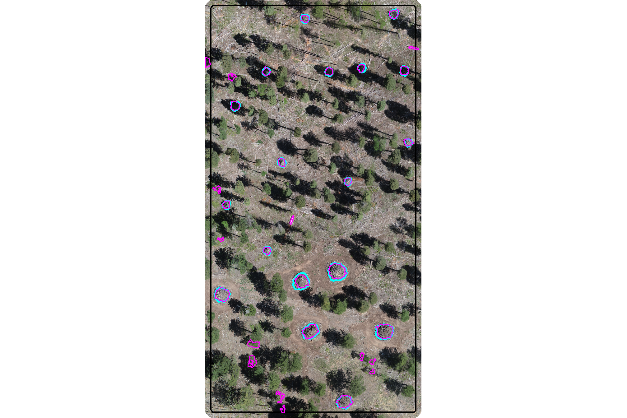
plot the filtered watershed candidate segments (magenta) and the actual piles (cyan) on the CHM
plt_aoi_chm(aoi_chm_rast_slice) +
  ggplot2::geom_sf(
    data = aoi_slash_piles_polys
    , fill = NA, color = "cyan", lwd = 0.6
  ) +
  ggplot2::geom_sf(
    data = watershed_segs_poly
    , fill = NA, color = "magenta", lwd = 0.6
  )
nice…we are getting closer.
4.3.2 DBSCAN Segmentation
plot the filtered dbscan candidate segments (magenta) and the actual piles (cyan) on the RGB
aoi_plt_ortho +
  ggplot2::geom_sf(data = aoi_boundary, fill = NA, color = "black", lwd = 0.8) +
  ggplot2::geom_sf(
    data = aoi_slash_piles_polys
    , fill = NA, color = "cyan", lwd = 0.9
  ) +
  ggplot2::geom_sf(
    data = dbscan_segs_poly
    , fill = NA, color = "magenta", lwd = 0.6
  ) +
  ggplot2::theme(legend.position = "none")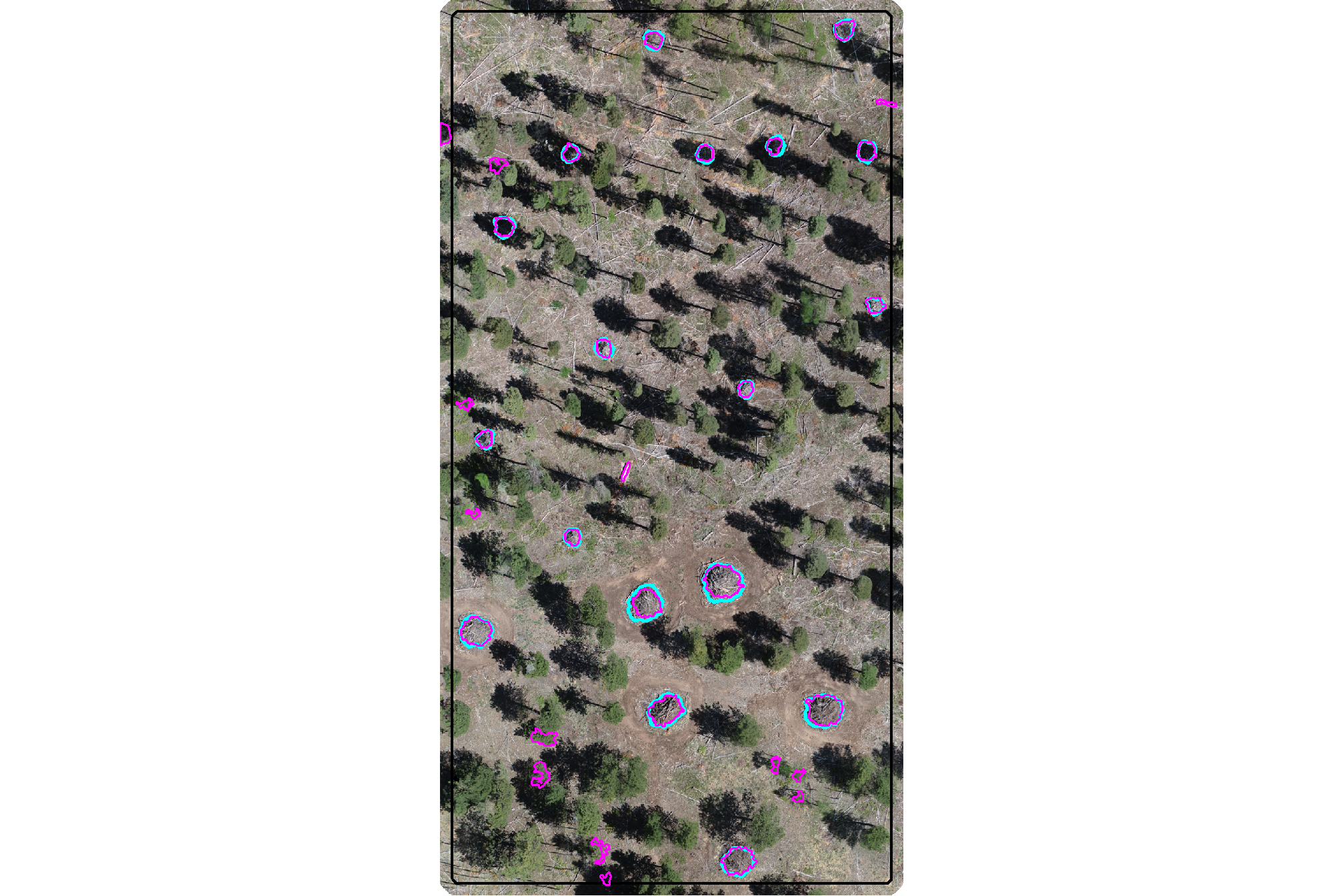
plot the filtered dbscan candidate segments (magenta) and the actual piles (cyan) on the CHM
plt_aoi_chm(aoi_chm_rast_slice) +
  ggplot2::geom_sf(
    data = aoi_slash_piles_polys
    , fill = NA, color = "cyan", lwd = 0.6
  ) +
  ggplot2::geom_sf(
    data = dbscan_segs_poly
    , fill = NA, color = "magenta", lwd = 0.6
  )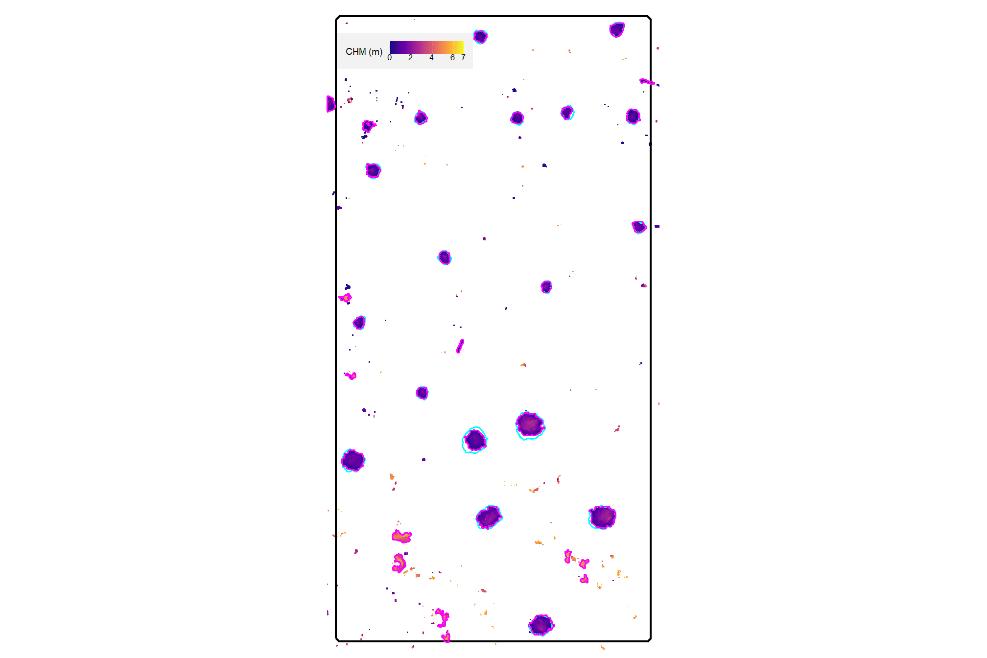
nice…we are getting closer.
4.3.3 Quick methods comparison
let’s quickly look at the watershed and dbscan segments on the same plot
ggplot2::ggplot() +
  ggplot2::geom_sf(
    data = watershed_segs_poly, mapping=ggplot2::aes(color="watershed")
    , fill = NA, lwd = 2
  ) +
  ggplot2::geom_sf(
    data = dbscan_segs_poly, mapping=ggplot2::aes(color="dbscan")
    , fill = NA, lwd = 1
  ) +
  ggplot2::scale_color_manual(values = c("gray33", "aquamarine3"),name="") +
  ggplot2::theme_void() +
  ggplot2::theme(legend.position = "top")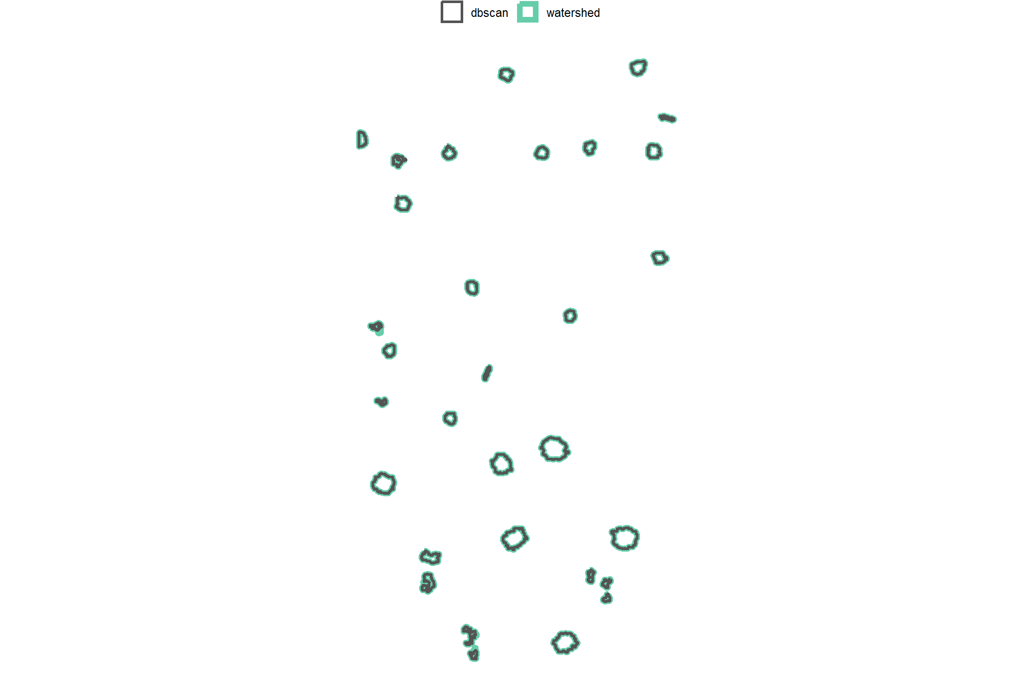
interesting.
4.4 Candidate Geometric filtering
slash piles are man-made objects typically constructed into common geometric forms in 2D (e.g. circular base) and 3D space (e.g. paraboloid) to facilitate efficient construction and burning Hardy 1996. Our method leverages these traits by applying independent geometric filters to refine candidate segments.
First, we apply a regularity filter to remove candidates with irregularly-shaped bases. Then, an independent circularity filter removes candidates that do not meet expectations for round bases (typical of hand piles). By keeping these filters independent, the our method is flexible and allows users to prioritize generally regular shapes (e.g. circular or rectangular) or apply the circularity filter as an additional filtering step when circular pile bases are expected.
4.4.1 Shape Irregularity: Convexity
Our first shape irregularity filter compares the convex hull of the candidate segment to the raw polygon of the candidate segment. Specifically, we calculate the convexity ratio or “solidity” of the shape (Glasbey and Horgan 1995) by:
\[\frac{\text{Area of Polygon}}{\text{Area of Convex Hull}}\]
This approach is effective for identifying polygons with deep indents, holes, or branching. A perfectly convex shape like a circle, square, or triangle will have a convexity of 1.0 (because they have no indents) and as shapes become more irregular (or concave) the convexity drops toward 0. Convexity is is not sensitive to the overall elongation of a shape as a long, thin rectangle is technically convex and would have a ratio of 1.0, despite being irregular in its proportions.
let’s create a convex hull of the candidate segments for comparison and convexity calculation
# convex hulls of segments
# watershed_segs_poly
watershed_segs_poly_chull <-
  watershed_segs_poly %>%
  sf::st_convex_hull() %>%
  sf::st_simplify() %>%
  sf::st_make_valid() %>%
  dplyr::filter(sf::st_is_valid(.))
# dbscan_segs_poly
dbscan_segs_poly_chull <-
  dbscan_segs_poly %>%
  sf::st_convex_hull() %>%
  sf::st_simplify() %>%
  sf::st_make_valid() %>%
  dplyr::filter(sf::st_is_valid(.))
compare the convex hull shape to the raw polygons
p1_temp <- ggplot2::ggplot() +
  ggplot2::geom_sf(
    data = watershed_segs_poly_chull, mapping=ggplot2::aes(color="convex hull")
    , fill = NA, lwd = 2
  ) +
  ggplot2::geom_sf(
    data = watershed_segs_poly, mapping=ggplot2::aes(color="raw polygons")
    , fill = NA, lwd = 1
  ) +
  ggplot2::scale_color_manual(values = c("orangered", "magenta"),name="") +
  ggplot2::labs(subtitle = "watershed") +
  ggplot2::theme_void() +
  ggplot2::theme(
    legend.position = "top"
    , plot.subtitle = ggplot2::element_text(hjust = 0.5)
    , panel.border = ggplot2::element_rect(color = "black", fill = NA, size = 1)
  )
p2_temp <- ggplot2::ggplot() +
  ggplot2::geom_sf(
    data = dbscan_segs_poly_chull, mapping=ggplot2::aes(color="convex hull")
    , fill = NA, lwd = 2
  ) +
  ggplot2::geom_sf(
    data = dbscan_segs_poly, mapping=ggplot2::aes(color="raw polygons")
    , fill = NA, lwd = 1
  ) +
  ggplot2::scale_color_manual(values = c("orangered", "magenta"),name="") +
  ggplot2::labs(subtitle = "dbscan") +
  ggplot2::theme_void() +
  ggplot2::theme(
    legend.position = "top"
    , plot.subtitle = ggplot2::element_text(hjust = 0.5)
    , panel.border = ggplot2::element_rect(color = "black", fill = NA, size = 1)
  )
patchwork::wrap_plots(list(p1_temp,p2_temp))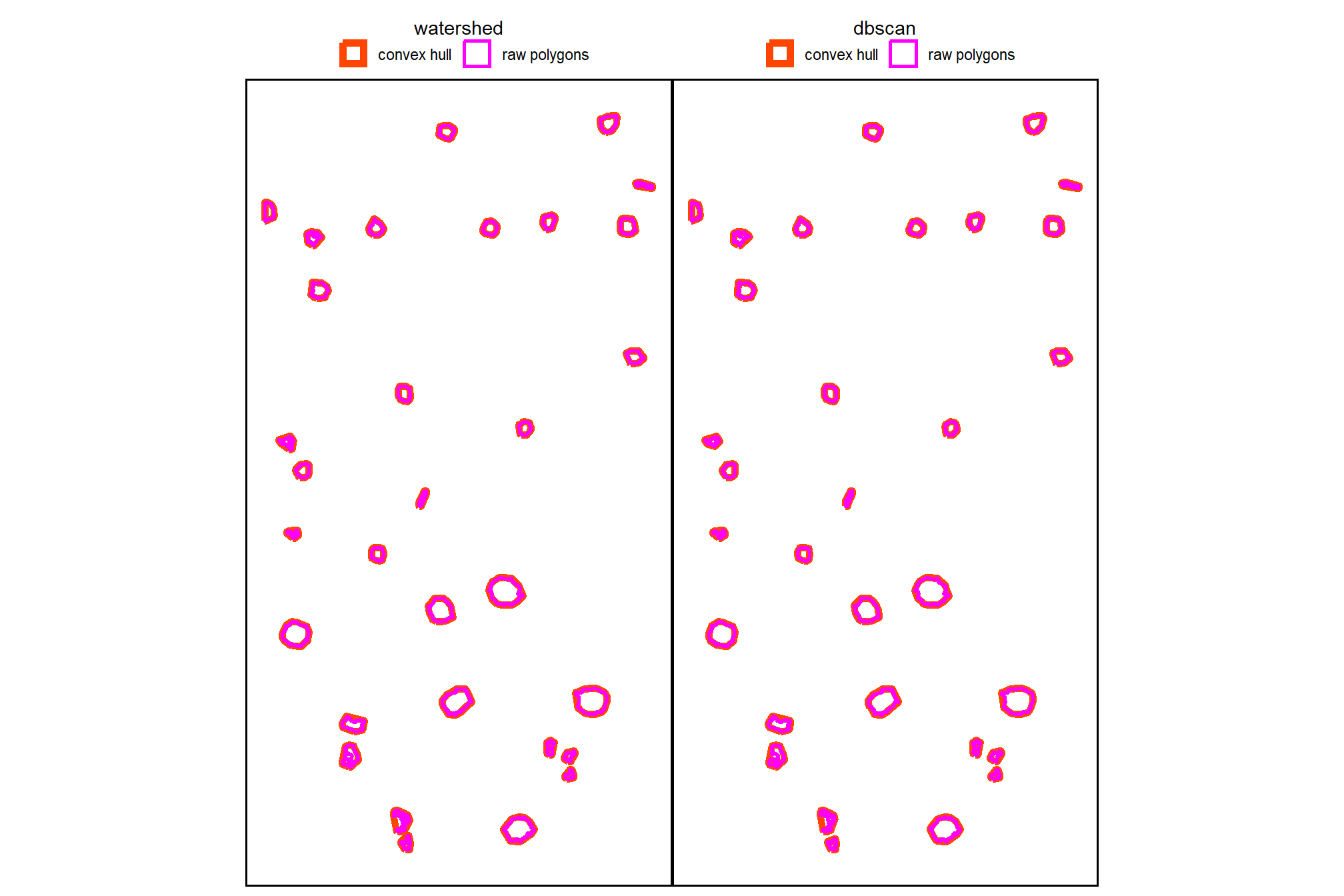
now, we’ll calculate the convexity ratio for each remaining candidate segment
# watershed_segs_poly
watershed_segs_poly <-
  watershed_segs_poly %>%
  dplyr::mutate(poly_area_m2 = sf::st_area(.) %>% as.numeric()) %>%
  dplyr::inner_join(
    watershed_segs_poly_chull %>%
      dplyr::mutate(chull_area_m2 = sf::st_area(.) %>% as.numeric()) %>%
      sf::st_drop_geometry() %>%
      dplyr::select(pred_id, chull_area_m2)
    , by = "pred_id"
  ) %>%
  dplyr::mutate(
    convexity_ratio = poly_area_m2/chull_area_m2
  )
# dbscan_segs_poly
dbscan_segs_poly <-
  dbscan_segs_poly %>%
  dplyr::mutate(poly_area_m2 = sf::st_area(.) %>% as.numeric()) %>%
  dplyr::inner_join(
    dbscan_segs_poly_chull %>%
      dplyr::mutate(chull_area_m2 = sf::st_area(.) %>% as.numeric()) %>%
      sf::st_drop_geometry() %>%
      dplyr::select(pred_id, chull_area_m2)
    , by = "pred_id"
  ) %>%
  dplyr::mutate(
    convexity_ratio = poly_area_m2/chull_area_m2
  )
what is the convexity ratio for the remaining candidate segments in our demonstration area?
##    Min. 1st Qu.  Median    Mean 3rd Qu.    Max.
## 0.4489 0.7686 0.8941 0.8310 0.9279 0.9423## Min. 1st Qu. Median Mean 3rd Qu. Max.
## 0.4591 0.7611 0.8941 0.8349 0.9279 0.9423plot the convexity of the candidate segments using the raw polygons
p1_temp <-
  ggplot2::ggplot() +
  ggplot2::geom_sf(
    data = watershed_segs_poly, mapping=ggplot2::aes(fill=convexity_ratio)
    , color = NA
  ) +
  ggplot2::geom_sf_text(
    data = watershed_segs_poly
    , mapping=ggplot2::aes(label=scales::percent(convexity_ratio, accuracy=0.1))
    , vjust = 1, hjust = 0, size = 3.5
  ) +
  ggplot2::scale_fill_fermenter(
    n.breaks = 10, palette = "PuOr"
    , direction = 1
    , limits = c(0,1)
    , labels = scales::percent
    , breaks = seq(0, 1, by = 0.2)
    , name = ""
  ) +
  ggplot2::labs(subtitle = "watershed") +
  ggplot2::theme_void() +
  ggplot2::theme(
    legend.position = "bottom"
    , plot.subtitle = ggplot2::element_text(hjust = 0.5)
    , panel.border = ggplot2::element_rect(color = "black", fill = NA, size = 1)
    , legend.text = ggplot2::element_text(size = 7)
  )
p2_temp <-
  ggplot2::ggplot() +
  ggplot2::geom_sf(
    data = dbscan_segs_poly, mapping=ggplot2::aes(fill=convexity_ratio)
    , color = NA
  ) +
  ggplot2::geom_sf_text(
    data = dbscan_segs_poly
    , mapping=ggplot2::aes(label=scales::percent(convexity_ratio, accuracy=0.1))
    , vjust = 1, hjust = 0, size = 3.5
  ) +
  ggplot2::scale_fill_fermenter(
    n.breaks = 10, palette = "PuOr"
    , direction = 1
    , limits = c(0,1)
    , labels = scales::percent
    , breaks = seq(0, 1, by = 0.2)
    , name = ""
  ) +
  ggplot2::labs(subtitle = "dbscan") +
  ggplot2::theme_void() +
  ggplot2::theme(
    legend.position = "bottom"
    , plot.subtitle = ggplot2::element_text(hjust = 0.5)
    , panel.border = ggplot2::element_rect(color = "black", fill = NA, size = 1)
    , legend.text = ggplot2::element_text(size = 7)
  )
patchwork::wrap_plots(
  list(p1_temp,p2_temp)
  , guides = "collect"
  ,
) &
ggplot2::theme(
    legend.position = "bottom"
    , legend.text = ggplot2::element_text(size = 7)
  )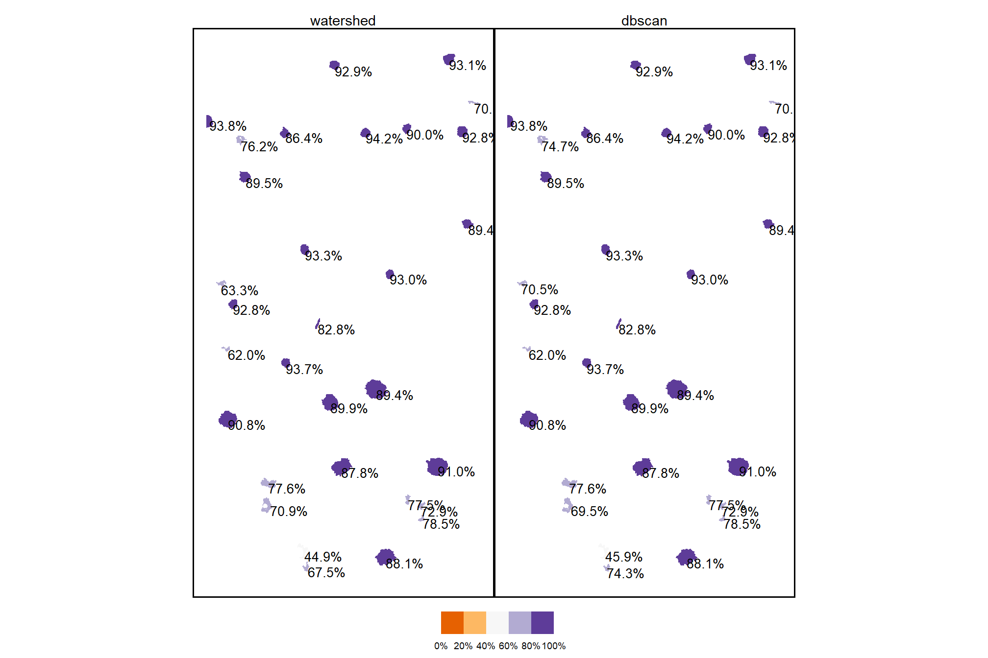
finally, let’s filter the candidate segments with a user-defined expectation of shape irregularity on the 0-100% scale applied to the convexity ratio
# # min required overlap between the predicted pile and the convex hull of the predicted pile
min_convexity_ratio <- 0.5
what proportion of the remaining segments were filtered using this shape irregularity filter
dplyr::tibble(
    method = c("watershed", "DBSCAN")
    , old_segments = c(
      watershed_segs_poly %>% nrow()
      , dbscan_segs_poly %>% nrow()
    )
    , new_segments = c(
      watershed_segs_poly %>% dplyr::filter(convexity_ratio>=min_convexity_ratio) %>% nrow()
      , dbscan_segs_poly %>% dplyr::filter(convexity_ratio>=min_convexity_ratio) %>% nrow()
    )
    , area = c(
      watershed_segs_poly %>%
        dplyr::filter(convexity_ratio>=min_convexity_ratio) %>%
        sf::st_union() %>%
        sf::st_area() %>%
        as.numeric()
      , dbscan_segs_poly %>%
        dplyr::filter(convexity_ratio>=min_convexity_ratio) %>%
        sf::st_union() %>%
        sf::st_area() %>%
        as.numeric()
    )
  ) %>%
  dplyr::mutate(
    pct_removed = scales::percent((new_segments-old_segments)/old_segments, accuracy = 0.1)
    , dplyr::across(tidyselect::ends_with("segments"), ~scales::comma(.x,accuracy=1))
    , area = scales::comma(area,accuracy=0.01)
  ) %>%
  dplyr::relocate(method,pct_removed) %>%
  kableExtra::kbl(
    caption = "Demonstration area candidate segments by method<br>filtered by segment convexity"
    , col.names = c(
      "method", "% removed"
      , "orig. candidate segments"
      , "filtered candidate segments"
      , "remaining candidate area (m<sup>2</sup>)"
    )
    , escape = F
  ) %>%
kableExtra::kable_styling()| method | % removed | orig. candidate segments | filtered candidate segments | remaining candidate area (m2) |
|---|---|---|---|---|
| watershed | -3.2% | 31 | 30 | 227.19 |
| DBSCAN | -3.2% | 31 | 30 | 226.62 |
actually apply the filter ;)
# watershed_segs_poly
watershed_segs_poly <- watershed_segs_poly %>%
  dplyr::filter(convexity_ratio>=min_convexity_ratio)
# dbscan_segs_poly
dbscan_segs_poly <- dbscan_segs_poly %>%
  dplyr::filter(convexity_ratio>=min_convexity_ratio)
4.4.1.1 Watershed Segmentation
plot the filtered watershed candidate segments (magenta) and the actual piles (cyan) on the RGB
aoi_plt_ortho +
  ggplot2::geom_sf(data = aoi_boundary, fill = NA, color = "black", lwd = 0.8) +
  ggplot2::geom_sf(
    data = aoi_slash_piles_polys
    , fill = NA, color = "cyan", lwd = 0.6
  ) +
  ggplot2::geom_sf(
    data = watershed_segs_poly
    , fill = NA, color = "magenta", lwd = 0.6
  ) +
  ggplot2::theme(legend.position = "none")
plot the filtered watershed candidate segments (magenta) and the actual piles (cyan) on the CHM
plt_aoi_chm(aoi_chm_rast_slice) +
  ggplot2::geom_sf(
    data = aoi_slash_piles_polys
    , fill = NA, color = "cyan", lwd = 0.6
  ) +
  ggplot2::geom_sf(
    data = watershed_segs_poly
    , fill = NA, color = "magenta", lwd = 0.6
  )
4.4.1.2 DBSCAN Segmentation
plot the filtered watershed candidate segments (magenta) and the actual piles (cyan) on the RGB
aoi_plt_ortho +
  ggplot2::geom_sf(data = aoi_boundary, fill = NA, color = "black", lwd = 0.8) +
  ggplot2::geom_sf(
    data = aoi_slash_piles_polys
    , fill = NA, color = "cyan", lwd = 0.6
  ) +
  ggplot2::geom_sf(
    data = dbscan_segs_poly
    , fill = NA, color = "magenta", lwd = 0.6
  ) +
  ggplot2::theme(legend.position = "none")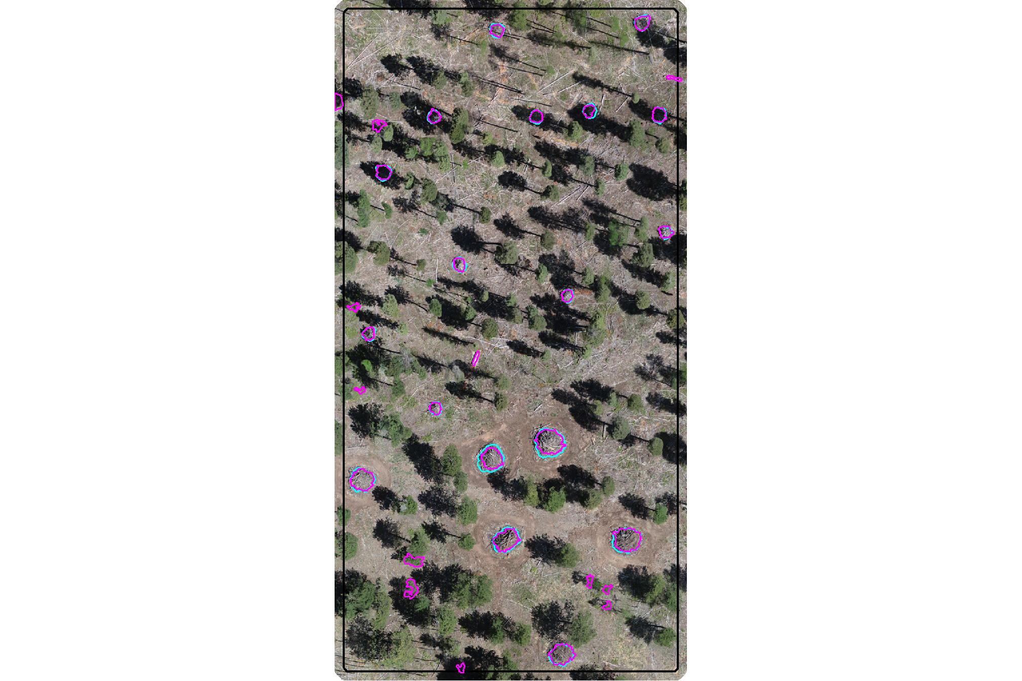
plot the filtered dbscan candidate segments (magenta) and the actual piles (cyan) on the CHM
plt_aoi_chm(aoi_chm_rast_slice) +
  ggplot2::geom_sf(
    data = aoi_slash_piles_polys
    , fill = NA, color = "cyan", lwd = 0.6
  ) +
  ggplot2::geom_sf(
    data = dbscan_segs_poly
    , fill = NA, color = "magenta", lwd = 0.6
  )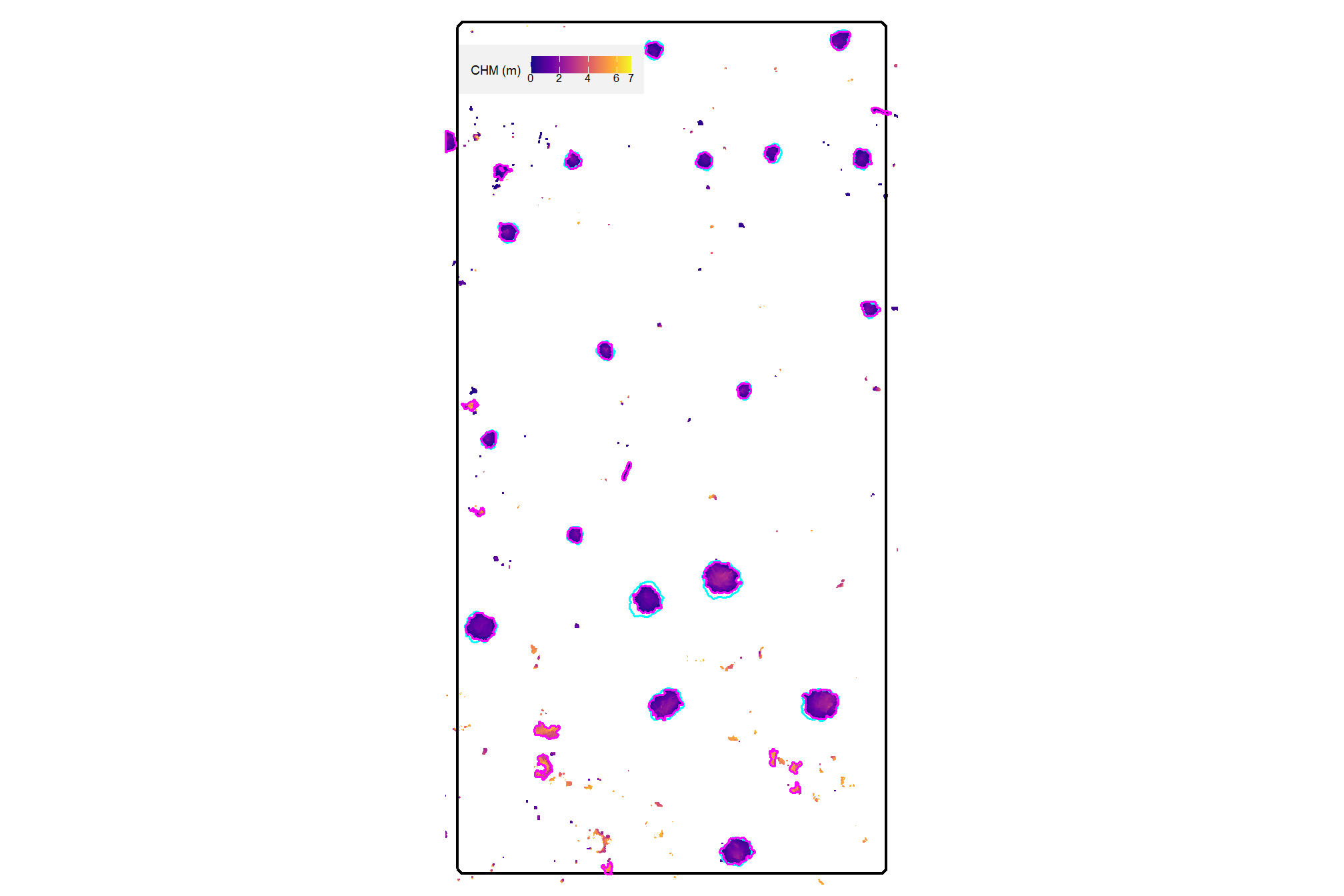
4.4.1.3 Convexity Filter Function
let’s make a function to ingest a spatial data frame and return polygons filtered for irregularity using this convex hull process
st_convexity_filter <- function(
  sf_data
  # min required overlap between the polygon and the convex hull of the polygon
  , min_convexity_ratio = 0.7
) {
  if(!inherits(sf_data, "sf")){stop("must pass `sf` data object")}
  # if not polygons
  if( !all(sf::st_is(sf_data, type = c("POLYGON", "MULTIPOLYGON"))) ){
    stop(paste0(
      "`sf_data` data must be an `sf` class object with POLYGON geometry (see [sf::st_geometry_type()])"
    ))
  }
  # convex hulls of segments
  poly_chull <-
    sf_data %>%
    sf::st_convex_hull() %>%
    sf::st_simplify() %>%
    sf::st_make_valid()
    # dplyr::filter(sf::st_is_valid(.))
  # compare areas
  if(nrow(poly_chull)!=nrow(sf_data)){
    stop("could not make valid convex hulls from provided polygon data")
  }else{
    area_comp <- sf_data %>%
      dplyr::mutate(area_xxxx = sf::st_area(.) %>% as.numeric()) %>%
      dplyr::bind_cols(
        poly_chull %>%
          dplyr::mutate(chull_area_xxxx = sf::st_area(.) %>% as.numeric()) %>%
          dplyr::select(chull_area_xxxx) %>%
          sf::st_drop_geometry()
      ) %>%
      dplyr::mutate(
        convexity_ratio = area_xxxx/chull_area_xxxx
      ) %>%
      dplyr::filter(
        convexity_ratio >= min_convexity_ratio
      ) %>%
      dplyr::select(-c(area_xxxx,chull_area_xxxx))
    return(area_comp)
  }
}
# dbscan_segs_poly$convexity_ratio %>% summary()
# dbscan_segs_poly %>%
#   st_convexity_filter(min_convexity_ratio = 0.9) %>%
#   dplyr::pull(convexity_ratio) %>%
#   summary()
4.4.2 Shape Irregularity: Circularity
Our second shape irregularity filter compares the minimum bounding circle of the candidate segment to the raw polygon of the candidate segment. Specifically, we calculate the circularity ratio sometimes referred to as the Reock Compactness Score (Reock 1961) of the shape by:
\[\frac{\text{Area of Polygon}}{\text{Area of Minumum Bounding Circle}}\]
This approach is used to measure how closely a shape is spread around its central point (dispersion) with a perfect circle receiving a score of 1.0 while long, thin shapes (like downed tree boles) will have low values approaching the lower limit of 0. This metric penalizes any shape that does not fill it’s circumcircle (i.e. the smallest circle that contains the polygon). For context, a perfect square has a circularity ratio of \(\frac{2}{\pi}\approx 0.637\) while an equilateral triangle has a ratio of \(\frac{3\sqrt{3}}{4\pi}\approx 0.414\)
let’s create the minimum bounding circle of the candidate segments using lwgeom::st_minimum_bounding_circle()
# MBC of segments
# watershed_segs_poly
watershed_segs_poly_mbc <-
  watershed_segs_poly %>%
  lwgeom::st_minimum_bounding_circle() %>%
  sf::st_simplify() %>%
  sf::st_make_valid() %>%
  dplyr::filter(sf::st_is_valid(.))
# dbscan_segs_poly
dbscan_segs_poly_mbc <-
  dbscan_segs_poly %>%
  lwgeom::st_minimum_bounding_circle() %>%
  sf::st_simplify() %>%
  sf::st_make_valid() %>%
  dplyr::filter(sf::st_is_valid(.))
compare the MBC shape to the raw polygons
p1_temp <- ggplot2::ggplot() +
  ggplot2::geom_sf(
    data = watershed_segs_poly_mbc, mapping=ggplot2::aes(color="min. bounding circle")
    , fill = NA, lwd = 1.5
  ) +
  ggplot2::geom_sf(
    data = watershed_segs_poly, mapping=ggplot2::aes(color="raw polygons")
    , fill = NA, lwd = 1
  ) +
  ggplot2::scale_color_manual(values = c("orangered", "magenta"),name="") +
  ggplot2::labs(subtitle = "watershed") +
  ggplot2::theme_void() +
  ggplot2::theme(
    legend.position = "top"
    , plot.subtitle = ggplot2::element_text(hjust = 0.5)
    , panel.border = ggplot2::element_rect(color = "black", fill = NA, size = 1)
  )
p2_temp <- ggplot2::ggplot() +
  ggplot2::geom_sf(
    data = dbscan_segs_poly_mbc, mapping=ggplot2::aes(color="min. bounding circle")
    , fill = NA, lwd = 1.5
  ) +
  ggplot2::geom_sf(
    data = dbscan_segs_poly, mapping=ggplot2::aes(color="raw polygons")
    , fill = NA, lwd = 1
  ) +
  ggplot2::scale_color_manual(values = c("orangered", "magenta"),name="") +
  ggplot2::labs(subtitle = "dbscan") +
  ggplot2::theme_void() +
  ggplot2::theme(
    legend.position = "top"
    , plot.subtitle = ggplot2::element_text(hjust = 0.5)
    , panel.border = ggplot2::element_rect(color = "black", fill = NA, size = 1)
  )
patchwork::wrap_plots(list(p1_temp,p2_temp))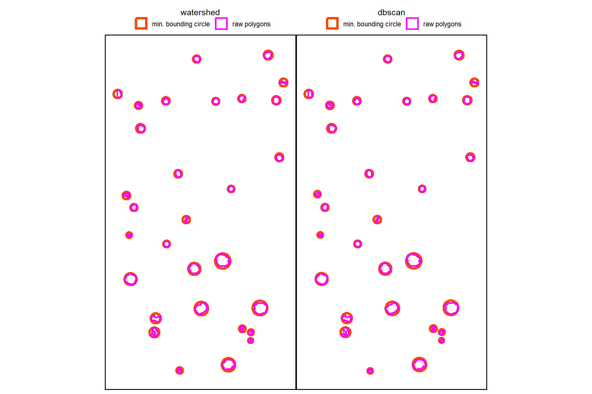
now, we’ll calculate the circularity ratio for each remaining candidate segment
# watershed_segs_poly
watershed_segs_poly <-
  watershed_segs_poly %>%
  dplyr::inner_join(
    watershed_segs_poly_mbc %>%
      dplyr::mutate(mbc_area_m2 = sf::st_area(.) %>% as.numeric()) %>%
      sf::st_drop_geometry() %>%
      dplyr::select(pred_id, mbc_area_m2)
    , by = "pred_id"
  ) %>%
  dplyr::mutate(
    circularity_ratio = poly_area_m2/mbc_area_m2
  )
# dbscan_segs_poly
dbscan_segs_poly <-
  dbscan_segs_poly %>%
  dplyr::inner_join(
    dbscan_segs_poly_mbc %>%
      dplyr::mutate(mbc_area_m2 = sf::st_area(.) %>% as.numeric()) %>%
      sf::st_drop_geometry() %>%
      dplyr::select(pred_id, mbc_area_m2)
    , by = "pred_id"
  ) %>%
  dplyr::mutate(
    circularity_ratio = poly_area_m2/mbc_area_m2
  )
what is the circularity ratio for the remaining candidate segments in our demonstration area?
##    Min. 1st Qu.  Median    Mean 3rd Qu.    Max.
## 0.1896 0.4700 0.6431 0.5770 0.6936 0.7991## Min. 1st Qu. Median Mean 3rd Qu. Max.
## 0.1896 0.4783 0.6431 0.5799 0.6936 0.7991plot the circularity of the candidate segments using the raw polygons
p1_temp <-
  ggplot2::ggplot() +
  ggplot2::geom_sf(
    data = watershed_segs_poly, mapping=ggplot2::aes(fill=circularity_ratio)
    , color = NA
  ) +
  ggplot2::geom_sf_text(
    data = watershed_segs_poly
    , mapping=ggplot2::aes(label=scales::percent(circularity_ratio, accuracy=0.1))
    , vjust = 1, hjust = 0, size = 3.5
  ) +
  ggplot2::scale_fill_fermenter(
    n.breaks = 10, palette = "PuOr"
    , direction = 1
    , limits = c(0,1)
    , labels = scales::percent
    , breaks = seq(0, 1, by = 0.2)
    , name = ""
  ) +
  ggplot2::labs(subtitle = "watershed") +
  ggplot2::theme_void() +
  ggplot2::theme(
    legend.position = "bottom"
    , plot.subtitle = ggplot2::element_text(hjust = 0.5)
    , panel.border = ggplot2::element_rect(color = "black", fill = NA, size = 1)
    , legend.text = ggplot2::element_text(size = 7)
  )
p2_temp <-
  ggplot2::ggplot() +
  ggplot2::geom_sf(
    data = dbscan_segs_poly, mapping=ggplot2::aes(fill=circularity_ratio)
    , color = NA
  ) +
  ggplot2::geom_sf_text(
    data = dbscan_segs_poly
    , mapping=ggplot2::aes(label=scales::percent(circularity_ratio, accuracy=0.1))
    , vjust = 1, hjust = 0, size = 3.5
  ) +
  ggplot2::scale_fill_fermenter(
    n.breaks = 10, palette = "PuOr"
    , direction = 1
    , limits = c(0,1)
    , labels = scales::percent
    , breaks = seq(0, 1, by = 0.2)
    , name = ""
  ) +
  ggplot2::labs(subtitle = "dbscan") +
  ggplot2::theme_void() +
  ggplot2::theme(
    legend.position = "bottom"
    , plot.subtitle = ggplot2::element_text(hjust = 0.5)
    , panel.border = ggplot2::element_rect(color = "black", fill = NA, size = 1)
    , legend.text = ggplot2::element_text(size = 7)
  )
patchwork::wrap_plots(
  list(p1_temp,p2_temp)
  , guides = "collect"
  ,
) &
ggplot2::theme(
    legend.position = "bottom"
    , legend.text = ggplot2::element_text(size = 7)
  )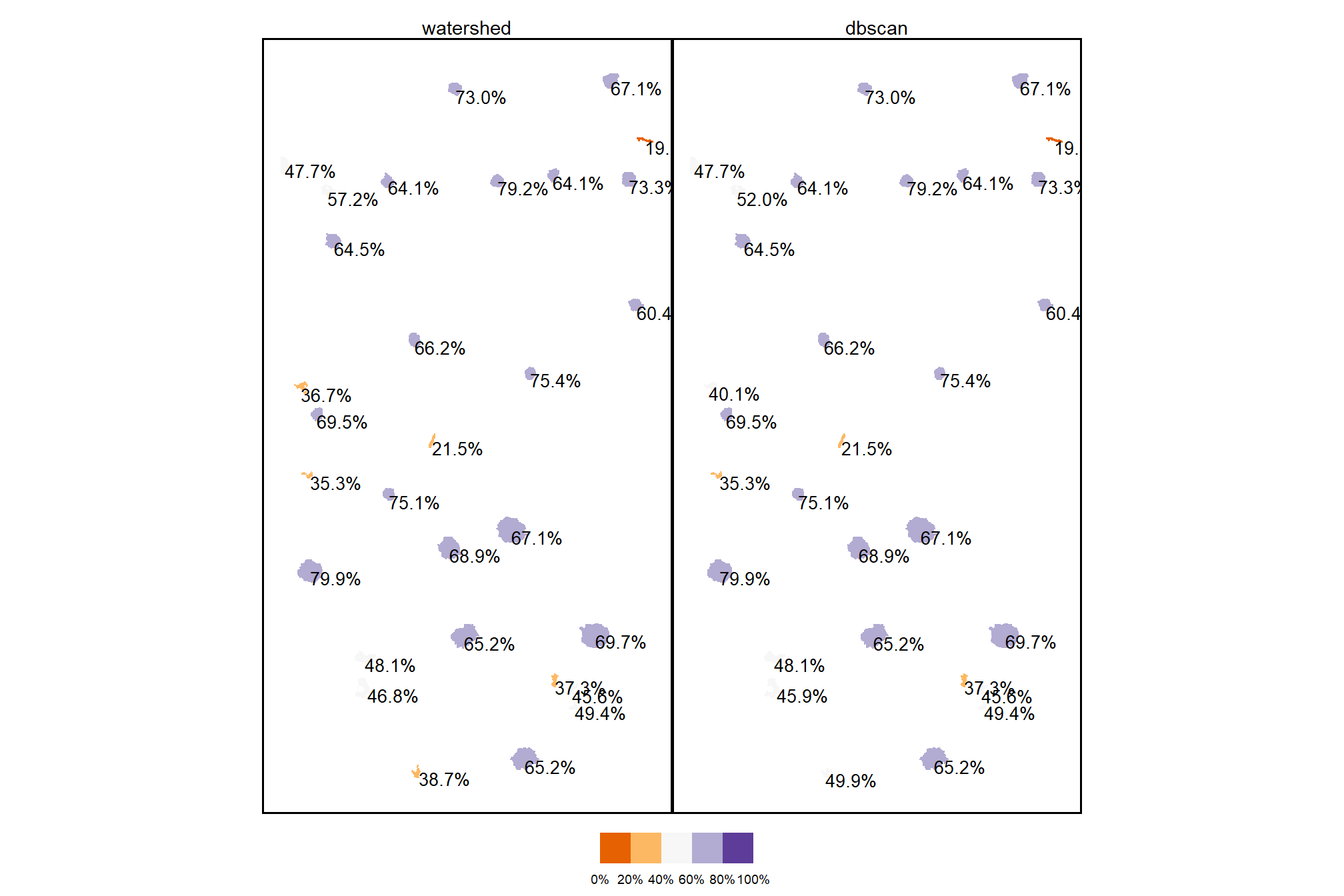
finally, let’s filter the candidate segments with a user-defined expectation of shape circularity on the 0-100% scale applied to the circularity ratio
# # min required overlap between the predicted pile and the MBC of the predicted pile
min_circularity_ratio <- 0.45
what proportion of the remaining segments were filtered using this shape circularity filter
dplyr::tibble(
    method = c("watershed", "DBSCAN")
    , old_segments = c(
      watershed_segs_poly %>% nrow()
      , dbscan_segs_poly %>% nrow()
    )
    , new_segments = c(
      watershed_segs_poly %>% dplyr::filter(circularity_ratio>=min_circularity_ratio) %>% nrow()
      , dbscan_segs_poly %>% dplyr::filter(circularity_ratio>=min_circularity_ratio) %>% nrow()
    )
    , area = c(
      watershed_segs_poly %>%
        dplyr::filter(circularity_ratio>=min_circularity_ratio) %>%
        sf::st_union() %>%
        sf::st_area() %>%
        as.numeric()
      , dbscan_segs_poly %>%
        dplyr::filter(circularity_ratio>=min_circularity_ratio) %>%
        sf::st_union() %>%
        sf::st_area() %>%
        as.numeric()
    )
  ) %>%
  dplyr::mutate(
    pct_removed = scales::percent((new_segments-old_segments)/old_segments, accuracy = 0.1)
    , dplyr::across(tidyselect::ends_with("segments"), ~scales::comma(.x,accuracy=1))
    , area = scales::comma(area,accuracy=0.01)
  ) %>%
  dplyr::relocate(method,pct_removed) %>%
  kableExtra::kbl(
    caption = "Demonstration area candidate segments by method<br>filtered by segment circularity"
    , col.names = c(
      "method", "% removed"
      , "orig. candidate segments"
      , "filtered candidate segments"
      , "remaining candidate area (m<sup>2</sup>)"
    )
    , escape = F
  ) %>%
kableExtra::kable_styling()| method | % removed | orig. candidate segments | filtered candidate segments | remaining candidate area (m2) |
|---|---|---|---|---|
| watershed | -20.0% | 30 | 24 | 214.18 |
| DBSCAN | -16.7% | 30 | 25 | 216.46 |
actually apply the filter ;)
# watershed_segs_poly
watershed_segs_poly <- watershed_segs_poly %>%
  dplyr::filter(circularity_ratio>=min_circularity_ratio)
# dbscan_segs_poly
dbscan_segs_poly <- dbscan_segs_poly %>%
  dplyr::filter(circularity_ratio>=min_circularity_ratio)
4.4.2.1 Watershed Segmentation
plot the filtered watershed candidate segments (magenta) and the actual piles (cyan) on the RGB
aoi_plt_ortho +
  ggplot2::geom_sf(data = aoi_boundary, fill = NA, color = "black", lwd = 0.8) +
  ggplot2::geom_sf(
    data = aoi_slash_piles_polys
    , fill = NA, color = "cyan", lwd = 0.6
  ) +
  ggplot2::geom_sf(
    data = watershed_segs_poly
    , fill = NA, color = "magenta", lwd = 0.6
  ) +
  ggplot2::theme(legend.position = "none")
plot the filtered watershed candidate segments (magenta) and the actual piles (cyan) on the CHM
plt_aoi_chm(aoi_chm_rast_slice) +
  ggplot2::geom_sf(
    data = aoi_slash_piles_polys
    , fill = NA, color = "cyan", lwd = 0.6
  ) +
  ggplot2::geom_sf(
    data = watershed_segs_poly
    , fill = NA, color = "magenta", lwd = 0.6
  )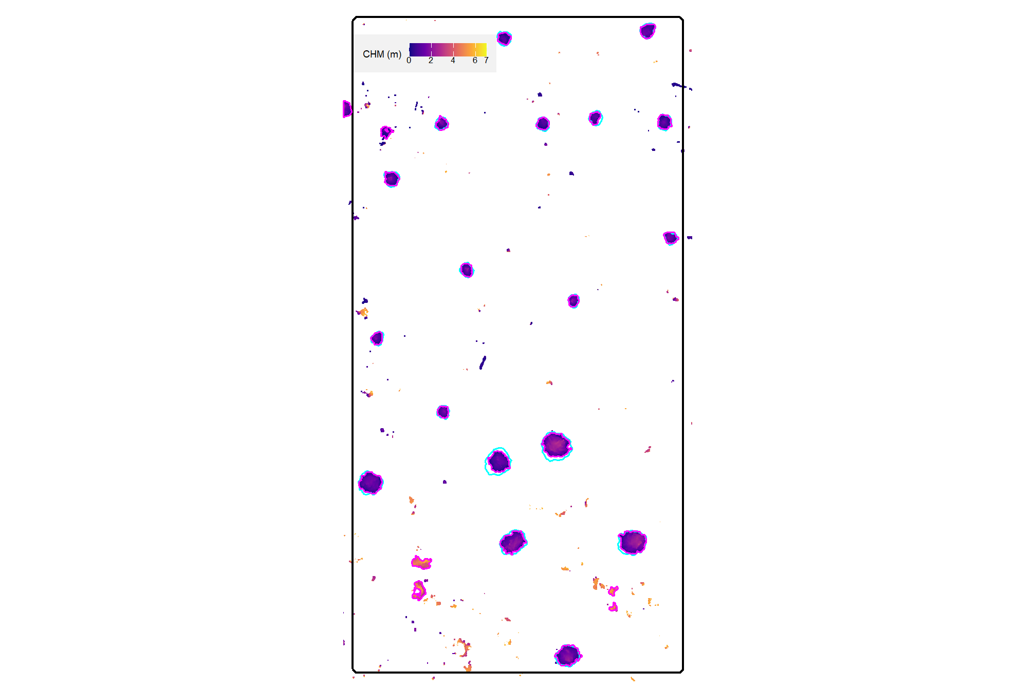
4.4.2.2 DBSCAN Segmentation
plot the filtered watershed candidate segments (magenta) and the actual piles (cyan) on the RGB
aoi_plt_ortho +
  ggplot2::geom_sf(data = aoi_boundary, fill = NA, color = "black", lwd = 0.8) +
  ggplot2::geom_sf(
    data = aoi_slash_piles_polys
    , fill = NA, color = "cyan", lwd = 0.6
  ) +
  ggplot2::geom_sf(
    data = dbscan_segs_poly
    , fill = NA, color = "magenta", lwd = 0.6
  ) +
  ggplot2::theme(legend.position = "none")
plot the filtered dbscan candidate segments (magenta) and the actual piles (cyan) on the CHM
plt_aoi_chm(aoi_chm_rast_slice) +
  ggplot2::geom_sf(
    data = aoi_slash_piles_polys
    , fill = NA, color = "cyan", lwd = 0.6
  ) +
  ggplot2::geom_sf(
    data = dbscan_segs_poly
    , fill = NA, color = "magenta", lwd = 0.6
  )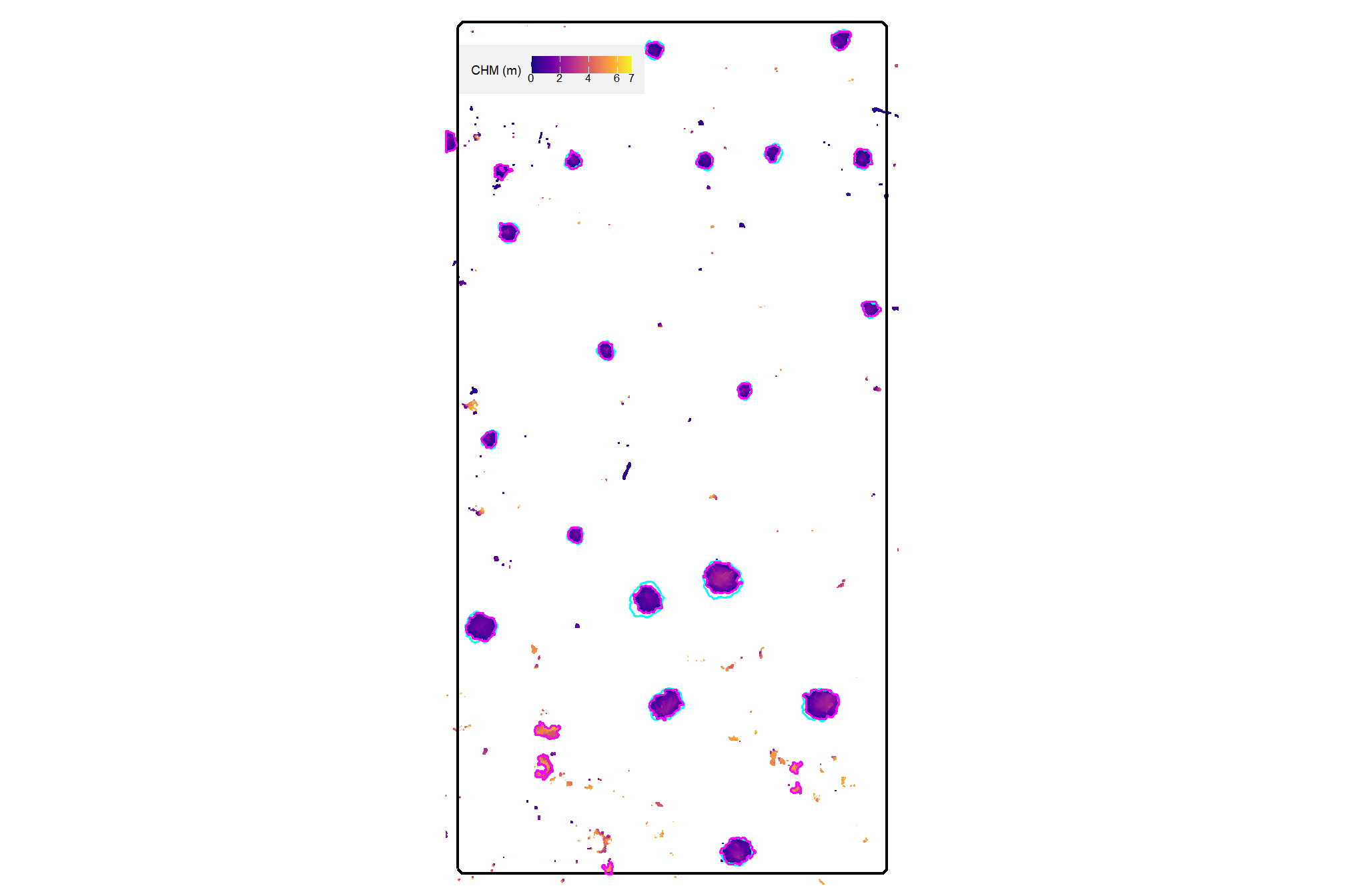
4.4.2.3 Circularity Filter Function
let’s make a function to ingest a spatial data frame and return polygons filtered for irregularity using this minimum bounding circle process
st_circularity_filter <- function(
  sf_data
  # min required overlap between the polygon and the minimum bounding circle of the polygon
  , min_circularity_ratio = 0.6
) {
  if(!inherits(sf_data, "sf")){stop("must pass `sf` data object")}
  # if not polygons
  if( !all(sf::st_is(sf_data, type = c("POLYGON", "MULTIPOLYGON"))) ){
    stop(paste0(
      "`sf_data` data must be an `sf` class object with POLYGON geometry (see [sf::st_geometry_type()])"
    ))
  }
  # minimum bounding circle of segments
  poly_mbc <-
    sf_data %>%
    lwgeom::st_minimum_bounding_circle() %>%
    sf::st_simplify() %>%
    sf::st_make_valid()
    # dplyr::filter(sf::st_is_valid(.))
  # compare areas
  if(nrow(poly_mbc)!=nrow(sf_data)){
    stop("could not make valid minimum bounding circle from provided polygon data")
  }else{
    area_comp <- sf_data %>%
      dplyr::mutate(area_xxxx = sf::st_area(.) %>% as.numeric()) %>%
      dplyr::bind_cols(
        poly_mbc %>%
          dplyr::mutate(mbc_area_xxxx = sf::st_area(.) %>% as.numeric()) %>%
          dplyr::select(mbc_area_xxxx) %>%
          sf::st_drop_geometry()
      ) %>%
      dplyr::mutate(
        circularity_ratio = area_xxxx/mbc_area_xxxx
      ) %>%
      dplyr::filter(
        circularity_ratio >= min_circularity_ratio
      ) %>%
      dplyr::select(-c(area_xxxx,mbc_area_xxxx))
    return(area_comp)
  }
}
# dbscan_segs_poly$circularity_ratio %>% summary()
# dbscan_segs_poly %>%
#   st_circularity_filter(min_circularity_ratio = 0.7) %>%
#   dplyr::pull(circularity_ratio) %>%
#   summary()
4.4.2.4 Quick methods comparison
let’s quickly look at the watershed and dbscan segments on the same plot now that we have removed candidate segments that 1) do not meet the area thresholds; 2) do not meet the convexity ratio threshold; and 3) do not meet the circularity ratio threshold
# watershed_segs_poly %>% dplyr::glimpse()
# dbscan_segs_poly %>% dplyr::glimpse()
ggplot2::ggplot() +
  ggplot2::geom_sf(
    data = watershed_segs_poly, mapping=ggplot2::aes(color="watershed")
    , fill = NA, lwd = 2
  ) +
  ggplot2::geom_sf(
    data = dbscan_segs_poly, mapping=ggplot2::aes(color="dbscan")
    , fill = NA, lwd = 1
  ) +
  ggplot2::scale_color_manual(values = c("gray33", "aquamarine3"),name="") +
  ggplot2::theme_void() +
  ggplot2::theme(legend.position = "top")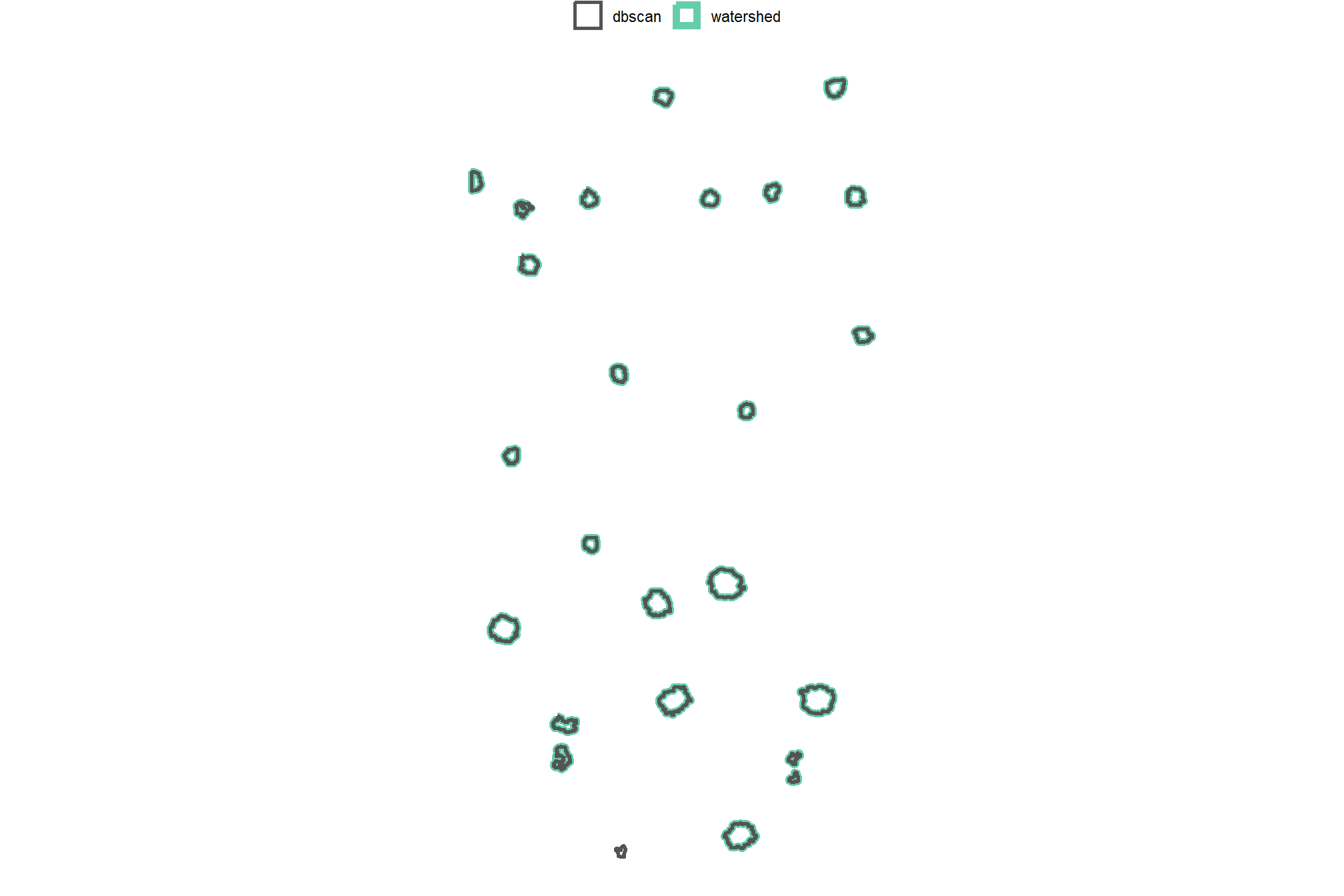
after all of that, the results of the two methods are essentially the same for this particular demonstration area
4.5 Structural Metrics from CHM
We’ll use the CHM raster to calculate area, height, and volume for each candidate pile to reflect the irregular pile footprints and elevation profiles that better represent real-world objects than assuming perfect geometric shapes like traditional pile measurement methods (Long and Boston, 2014; Trofymow et al., 2014; Guth et al., 2025)
Candidate slash pile structural metrics are derived from the CHM raster using zonal statistics to aggregate cell-level raster data within the boundaries of each pile. To ensure geodetic accuracy, an area raster is generated (terra::cellSize()) which accounts for minute variations in pixel area caused by the curvature of the Earth and the coordinate reference system. This area raster is then used as input for volume calculation, where it is multiplied by the CHM height values to create a volume raster. Summing the individual volume of every pixel within the candidate pile footprint yields the total pile volume with each cell in the volume raster treated as a rectangular prism with height from the CHM and base area from the area raster. Pile area is calculated by summing the area raster values within the candidate pile boundary and pile height is determined by the maximum CHM pixel value.
we’ll make a function to use polygon sf data and an input CHM raster to perform these calculations and return the data with metrics attached
########################################################################################
## calculate raster-based area, height, and volume using zonal stats
########################################################################################
get_structural_metrics <- function(
    sf_data
    , chm_rast
    # , sf_id = NA
) {
  # check polygons
  if(!inherits(sf_data, "sf")){stop("must include `sf` data object in 'sf_data'")}
  if( !all(sf::st_is(sf_data, type = c("POLYGON", "MULTIPOLYGON"))) ){
    stop(paste0(
      "`sf_data` data must be an `sf` class object with POLYGON geometry (see [sf::st_geometry_type()])"
    ))
  }
  sf_data <- sf_data %>% dplyr::ungroup()

  # check raster
  # convert to SpatRaster if input is from 'raster' package
  if(
    inherits(chm_rast, "RasterStack")
    || inherits(chm_rast, "RasterBrick")
  ){
    chm_rast <- terra::rast(chm_rast)
  }else if(!inherits(chm_rast, "SpatRaster")){
    stop("Input 'chm_rast' must be a SpatRaster from the `terra` package")
  }
  chm_rast <- chm_rast %>% terra::subset(subset = 1)
  if(
    as.numeric(terra::global(chm_rast, fun = "isNA")) == terra::ncell(chm_rast)
    # || as.numeric(terra::global(chm_rast, fun = "isNA")) >= round(terra::ncell(chm_rast)*0.98)
  ){
    stop("Input 'chm_rast' has all missing values")
  }

  # # check id
  # if(!inherits(sf_id, "character")){
  #   # stop("must include 'sf_id' as the unique identifier")
  #   sf_data <- sf_data %>%
  #     dplyr::mutate(idxxxxx = dplyr::row_number())
  #   sf_id <- "idxxxxx"
  # }else{
  #   if( !any( stringr::str_equal(names(sf_data), sf_id) ) ){
  #     stop(paste0("could not locate '",sf_id,"' in sf_data"))
  #   }
  # }

  # check overlap
  # Returns TRUE if any part of the vector geometry intersects the raster extent
  if(
    !any(terra::is.related(
      x = sf_data %>%
        sf::st_transform(terra::crs(chm_rast)) %>%
        terra::vect()
      , y = terra::ext(chm_rast)
      , relation = "intersects"
    ))
  ){
    stop("Input 'sf_data' does not overlap with 'chm_rast'")
  }
  #################################
  # area, volume of each cell
  #################################
  area_rast_temp <- terra::cellSize(chm_rast)
  names(area_rast_temp) <- "area_m2"
  # area_rast_temp %>% terra::plot()
  # then, multiply area by the CHM (elevation) for each cell to get a raster with cell volumes
  vol_rast_temp <- area_rast_temp*chm_rast
  names(vol_rast_temp) <- "volume_m3"
  # vol_rast_temp %>% terra::plot()
  #################################
  # zonal stats
  #################################
  # sum area within each segment to get the total area
  area_df_temp <- terra::zonal(
      x = area_rast_temp
      , z = sf_data %>%
        sf::st_transform(terra::crs(chm_rast)) %>%
        terra::vect()
      , fun = "sum", na.rm = T
    ) %>%
    setNames("area_m2") %>%
    dplyr::mutate(area_m2 = dplyr::na_if(area_m2, NaN))
  # area_df_temp %>% dplyr::glimpse()
  # sum volume within each segment to get the total volume
  vol_df_temp <- terra::zonal(
      x = vol_rast_temp
      , z = sf_data %>%
        sf::st_transform(terra::crs(chm_rast)) %>%
        terra::vect()
      , fun = "sum", na.rm = T
    ) %>%
    setNames("volume_m3") %>%
    dplyr::mutate(volume_m3 = dplyr::na_if(volume_m3, NaN))
  # vol_df_temp %>% dplyr::glimpse()
  # max ht within each segment to get the max ht
  ht_df_temp <- terra::zonal(
      x = chm_rast
      , z = sf_data %>%
        sf::st_transform(terra::crs(chm_rast)) %>%
        terra::vect()
      , fun = "max", na.rm = T
    ) %>%
    setNames("max_height_m") %>%
    dplyr::mutate(max_height_m = dplyr::na_if(max_height_m, NaN))
  #################################
  # attach to sf
  #################################
  if(
    !identical(
      nrow(sf_data)
      , nrow(area_df_temp)
      , nrow(vol_df_temp)
      , nrow(ht_df_temp)
    )
  ){
    stop("unable to find data in raster for given vectors")
  }

  ret_dta <- sf_data %>%
    dplyr::select( -dplyr::any_of(c(
      "hey_xxxxxxxxxx"
      , "area_m2"
      , "volume_m3"
      , "max_height_m"
      , "volume_per_area"
    ))) %>%
    dplyr::bind_cols(
      area_df_temp
      , vol_df_temp
      , ht_df_temp
    ) %>%
    dplyr::mutate(
      volume_per_area = volume_m3/area_m2
    )
  # ret_dta <- sf_data %>%
  #   purrr::reduce(
  #     list(sf_data, area_df_temp, vol_df_temp, ht_df_temp)
  #     , dplyr::left_join
  #     , by = sf_id
  #   ) %>%
  #   dplyr::mutate(
  #     volume_per_area = volume_m3/area_m2
  #   )

  return(
    list(
      sf_data = ret_dta
      , area_rast = area_rast_temp
      , volume_rast = vol_rast_temp
    )
  )
}

# get_structural_metrics(sf_data = watershed_segs_poly, chm_rast = aoi_chm_rast_slice) %>%
#   dplyr::glimpse()
# get_structural_metrics(sf_data = watershed_segs_poly, chm_rast = arnf_chm_rast) %>%
#   dplyr::glimpse()
4.5.1 Structural Rasters
we can quickly look at the area raster that was used for the volume calculation
get_structural_metrics(sf_data = watershed_segs_poly, chm_rast = aoi_chm_rast_slice) %>%
  purrr::pluck("area_rast") %>%
  terra::plot(axes = F, col = grDevices::gray.colors(n=100), main = "area (m2)")
and we can quickly look at the volume raster
get_structural_metrics(sf_data = watershed_segs_poly, chm_rast = aoi_chm_rast_slice) %>%
  purrr::pluck("volume_rast") %>%
  terra::plot(axes = F, col = grDevices::gray.colors(n=100), main = "volume (m3)")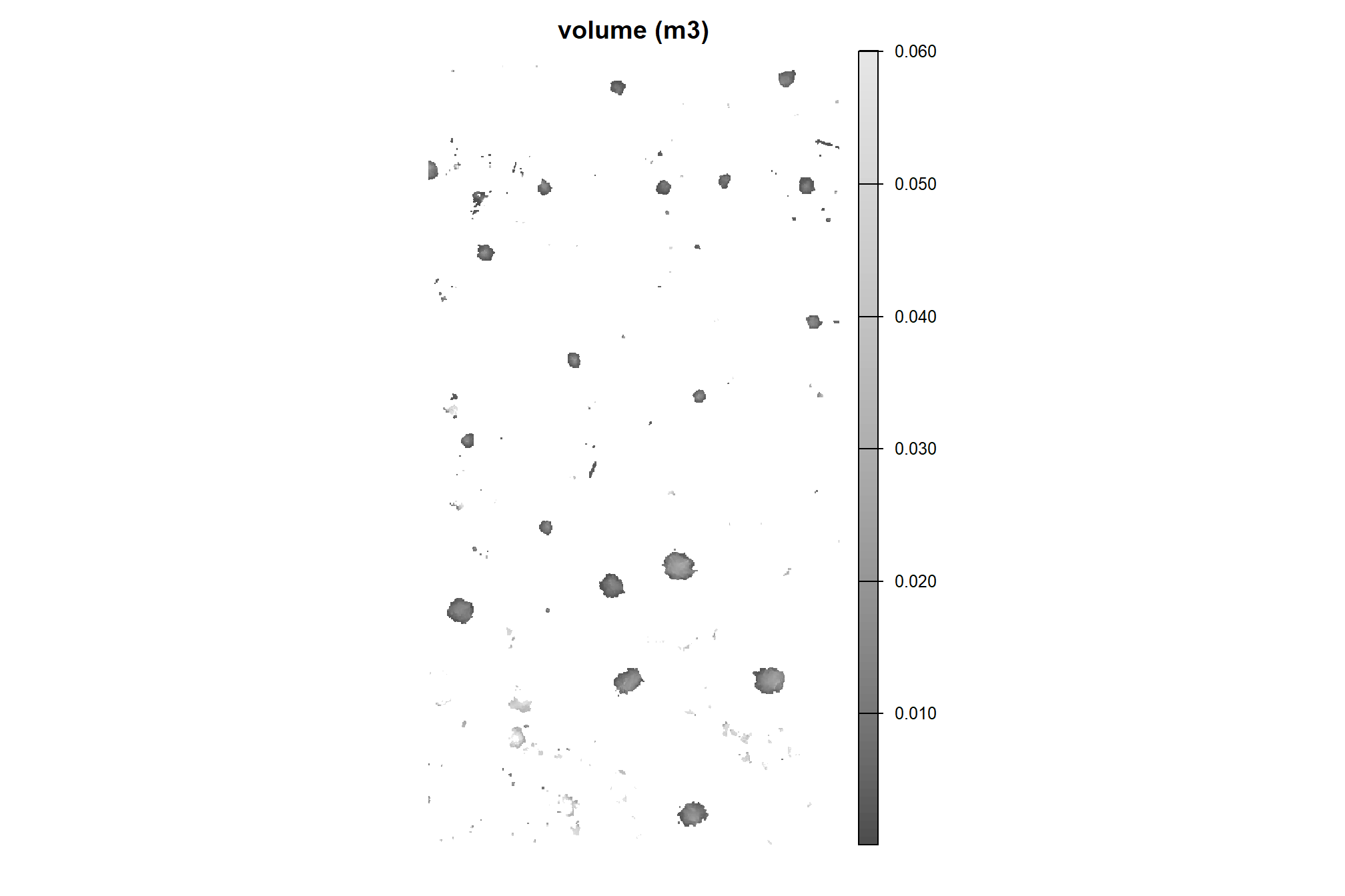
# terra::plot(
#   aoi_slash_piles_polys %>%
#     sf::st_transform(terra::crs(aoi_chm_rast_slice)) %>%
#     terra::vect()
#   , add = T, border = "cyan", col = NA, lwd = 1.2
# )
the volume raster mirrors the CHM but with volume as the cell value instead of height
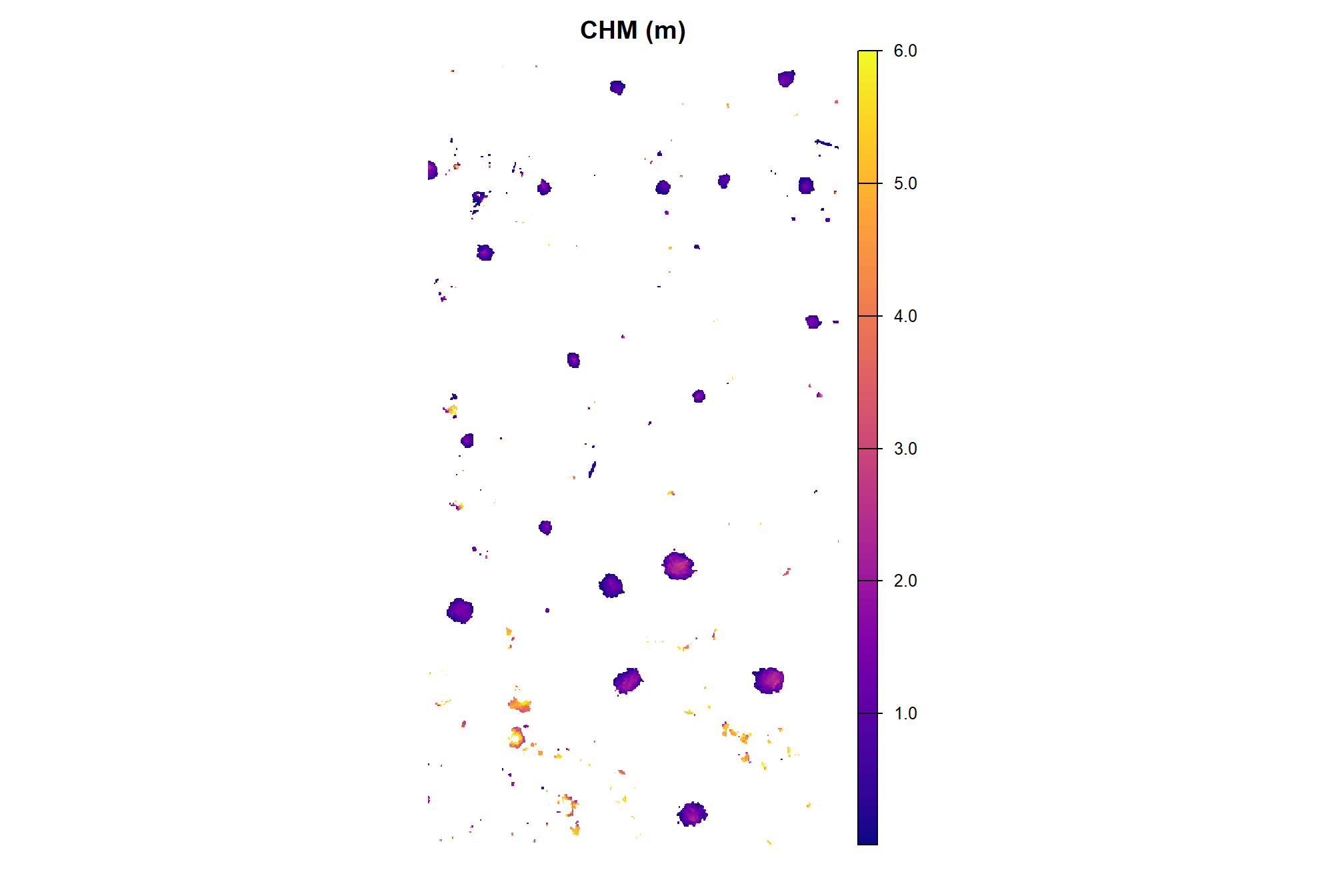
4.5.2 Demonstration Candidate Segment Metrics
we’ll use our get_structural_metrics() with the height-filtered CHM to compute the structural metrics for the candidate piles
# watershed_segs_poly
watershed_segs_poly <- get_structural_metrics(sf_data = watershed_segs_poly, chm_rast = aoi_chm_rast_slice) %>%
  purrr::pluck("sf_data") %>%
  # we already have area so we'll drop the value from this function
  dplyr::select( -dplyr::any_of(c(
    "hey_xxxxxxxxxx"
    , "poly_area_m2"
  )))
# dbscan_segs_poly
dbscan_segs_poly <- get_structural_metrics(sf_data = dbscan_segs_poly, chm_rast = aoi_chm_rast_slice) %>%
  purrr::pluck("sf_data") %>%
  # we already have area so we'll drop the value from this function
  dplyr::select( -dplyr::any_of(c(
    "hey_xxxxxxxxxx"
    , "poly_area_m2"
  )))
what did we get back?
## Rows: 24
## Columns: 10
## $ pred_id           <dbl> 22, 133, 135, 141, 142, 143, 145, 146, 147, 151, 156…
## $ chull_area_m2     <dbl> 9.495, 25.320, 26.820, 5.275, 5.055, 20.255, 6.175, …
## $ convexity_ratio   <dbl> 0.7761980, 0.9095577, 0.8941089, 0.9383886, 0.929772…
## $ mbc_area_m2       <dbl> 15.316338, 33.030222, 35.734991, 10.370370, 6.234503…
## $ circularity_ratio <dbl> 0.4811855, 0.6972402, 0.6710510, 0.4773215, 0.753869…
## $ area_m2           <dbl> 7.375899, 23.048435, 23.999195, 4.953962, 4.703762, …
## $ volume_m3         <dbl> 32.331139, 31.446938, 35.541131, 5.187639, 4.081403,…
## $ max_height_m      <dbl> 5.965939, 3.566000, 3.181000, 2.578000, 2.559000, 2.…
## $ volume_per_area   <dbl> 4.3833487, 1.3643850, 1.4809301, 1.0471696, 0.867689…
## $ geometry          <POLYGON [m]> POLYGON ((499326 4317738, 4..., POLYGON ((49…
plot the metrics of pile area, height, and volume
# p1_temp <-
p_fn_temp <- function(dta,fill_col,col_nm=latex2exp::TeX("area $\\textrm{m}^2$"),pal="Oranges"){
  ggplot2::ggplot(data = dta) +
  ggplot2::geom_sf(
    mapping=ggplot2::aes(fill=.data[[fill_col]])
    # mapping=ggplot2::aes(fill={{fill_col}})
    , color = NA
  ) +
  ggplot2::geom_sf_text(
    # mapping=ggplot2::aes(label=scales::comma({{fill_col}}, accuracy=0.1))
    mapping=ggplot2::aes(label=scales::comma(.data[[fill_col]], accuracy=0.1))
    , vjust = 1, hjust = -0.9, size = 2.5
  ) +
  ggplot2::scale_fill_distiller(palette = pal, name = col_nm, direction = 1) +
  ggplot2::labs(subtitle = col_nm) +
  ggplot2::theme_void() +
  ggplot2::theme(
    legend.position = "top", legend.direction = "horizontal"
    , legend.title = ggplot2::element_blank()
    , plot.subtitle = ggplot2::element_text(size = 6, hjust = 0.5)
    , panel.border = ggplot2::element_rect(color = "black", fill = NA, size = 1)
    , legend.text = ggplot2::element_text(size = 7)
  )
}
# lists
pal_temp <- c("Blues","Purples","Greens")
nm_temp <- c(
  latex2exp::TeX("area $\\textrm{m}^2$")
  , latex2exp::TeX("volume $\\textrm{m}^3$")
  , "height m"
)
col_temp <- c(
  "area_m2"
  , "volume_m3"
  , "max_height_m"
)
# watershed
ws_p_temp <- 1:length(col_temp) %>%
  purrr::map(
    \(x)
    p_fn_temp(
      watershed_segs_poly
      , fill_col = col_temp[x]
      , col_nm = nm_temp[x]
      , pal = pal_temp[x]
    )
  )
# dbscan
db_p_temp <- 1:length(col_temp) %>%
  purrr::map(
    \(x)
    p_fn_temp(
      dbscan_segs_poly
      , fill_col = col_temp[x]
      , col_nm = nm_temp[x]
      , pal = pal_temp[x]
    )
  )
p1_temp <- patchwork::wrap_plots(
    ws_p_temp
  ) +
  patchwork::plot_annotation(
    title = "watershed"
    , theme = ggplot2::theme(plot.title = ggplot2::element_text(size = 14))
  )
p2_temp <- patchwork::wrap_plots(
    db_p_temp
  ) +
  patchwork::plot_annotation(
    title = "dbscan"
    , theme = ggplot2::theme(plot.title = ggplot2::element_text(size = 14))
  )

patchwork::wrap_plots(
  list(
    patchwork::wrap_elements( p1_temp )
    , patchwork::wrap_elements( p2_temp )
  )
  , nrow = 2
)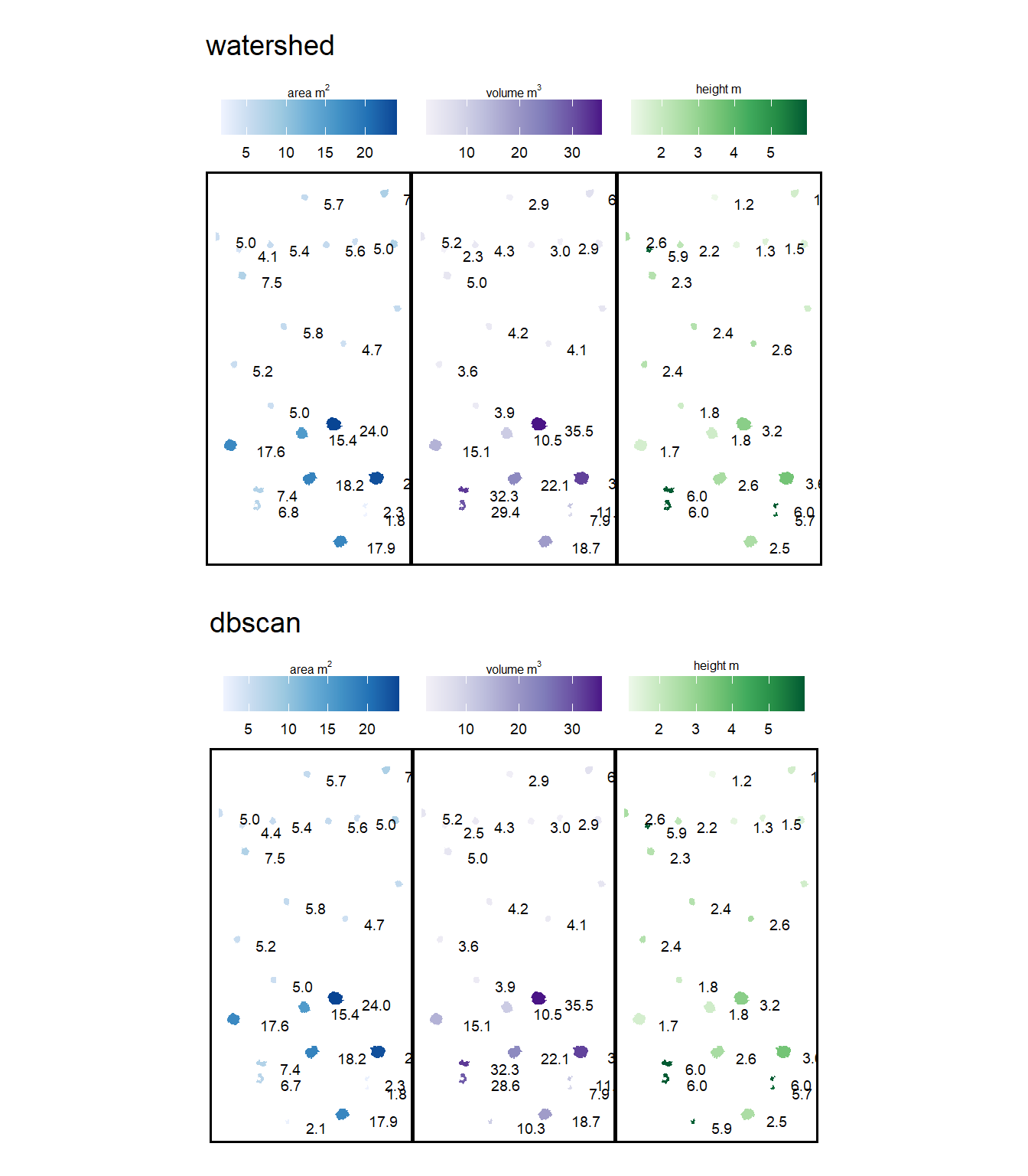
after all of that, the results of the two methods are the same for this particular demonstration area
4.6 Final Shape Refinement
In the final stage, we generate convex hulls for the segments to smooth the blocky, pixelated edges inherent in raster data (which can look like they were generated in Minecraft). Any segments with overlapping convex hulls are then removed to help filter out false detections which may be groups of small trees or shrubs. This step is intended to reflect real-world conditions where distinct slash piles are constructed with enough spacing to remain spatially independent rather than overlapping. Finally, we’ll apply one more filter for the area and height thresholds.
###############################################################################
# make a function to remove overlapping polygons from a sf data frame
###############################################################################
st_remove_overlaps <- function(sf_data) {
  if(!inherits(sf_data, "sf")){stop("must pass `sf` data object")}
  # if not polygons
  if( !all(sf::st_is(sf_data, type = c("POLYGON", "MULTIPOLYGON"))) ){
    stop(paste0(
      "`sf_data` data must be an `sf` class object with POLYGON geometry (see [sf::st_geometry_type()])"
    ))
  }
  if(nrow(sf_data)<=1){return(sf_data)}
  # combine all touching polygons and keep the ones that overlap multiple from the original polygons
  comb_temp <- sf_data %>%
    dplyr::ungroup() %>%
    sf::st_union(by_feature = F) %>%
    sf::st_cast("POLYGON") %>%
    sf::st_as_sf() %>%
    sf::st_set_geometry("geometry") %>%
    sf::st_set_crs(sf::st_crs(sf_data)) %>%
    dplyr::mutate(new_id = dplyr::row_number()) %>%
    dplyr::select(new_id)
  # identify overlaps
  overlap_temp <- comb_temp %>%
    sf::st_intersection(sf_data) %>%
    sf::st_drop_geometry() %>%
    dplyr::group_by(new_id) %>%
    dplyr::summarise(n_orig = dplyr::n()) %>%
    dplyr::ungroup() %>%
    dplyr::filter(n_orig>=2) %>%
    dplyr::pull(new_id)
  if(length(overlap_temp)==0){return(sf_data)}
  # just get the overlaps
  comb_temp <- comb_temp %>%
    dplyr::filter(new_id %in% overlap_temp) %>%
    sf::st_union()
  # remove all input polygons from the original data that have any overlaps
  return(sf::st_difference(sf_data,comb_temp))
}
take the convex hull and apply our st_remove_overlaps() function to the remaining candidate segments. Finally, we filter for area based on the smoothed shape
# watershed_segs_poly
watershed_segs_poly <-
  watershed_segs_poly %>%
  sf::st_convex_hull() %>%
  sf::st_simplify() %>%
  sf::st_make_valid() %>%
  dplyr::filter(sf::st_is_valid(.)) %>%
  st_remove_overlaps() %>%
  # now we need to re-do the volume and area calculations
  dplyr::mutate(
    area_m2 = sf::st_area(.) %>% as.numeric()
    , volume_m3 = area_m2*volume_per_area
  ) %>%
  st_filter_area(min_area_m2 = min_area_m2, max_area_m2 = max_area_m2) %>%
  # filter for height
  dplyr::filter(
    max_height_m >= min_ht_m
    & max_height_m <= max_ht_m
  )
# dbscan_segs_poly
dbscan_segs_poly <-
  dbscan_segs_poly %>%
  sf::st_convex_hull() %>%
  sf::st_simplify() %>%
  sf::st_make_valid() %>%
  dplyr::filter(sf::st_is_valid(.)) %>%
  st_remove_overlaps() %>%
  # now we need to re-do the volume and area calculations
  dplyr::mutate(
    area_m2 = sf::st_area(.) %>% as.numeric()
    , volume_m3 = area_m2*volume_per_area
  ) %>%
  st_filter_area(min_area_m2 = min_area_m2, max_area_m2 = max_area_m2) %>%
  # filter for height
  dplyr::filter(
    max_height_m >= min_ht_m
    & max_height_m <= max_ht_m
  )
# dbscan_segs_poly %>% dplyr::glimpse()
4.6.1 Watershed Segmentation
plot the filtered watershed candidate segments (magenta) and the actual piles (cyan) on the RGB
aoi_plt_ortho +
  ggplot2::geom_sf(data = aoi_boundary, fill = NA, color = "black", lwd = 0.8) +
  ggplot2::geom_sf(
    data = aoi_slash_piles_polys
    , fill = NA, color = "cyan", lwd = 0.6
  ) +
  ggplot2::geom_sf(
    data = watershed_segs_poly
    , fill = NA, color = "magenta", lwd = 0.6
  ) +
  ggplot2::theme(legend.position = "none")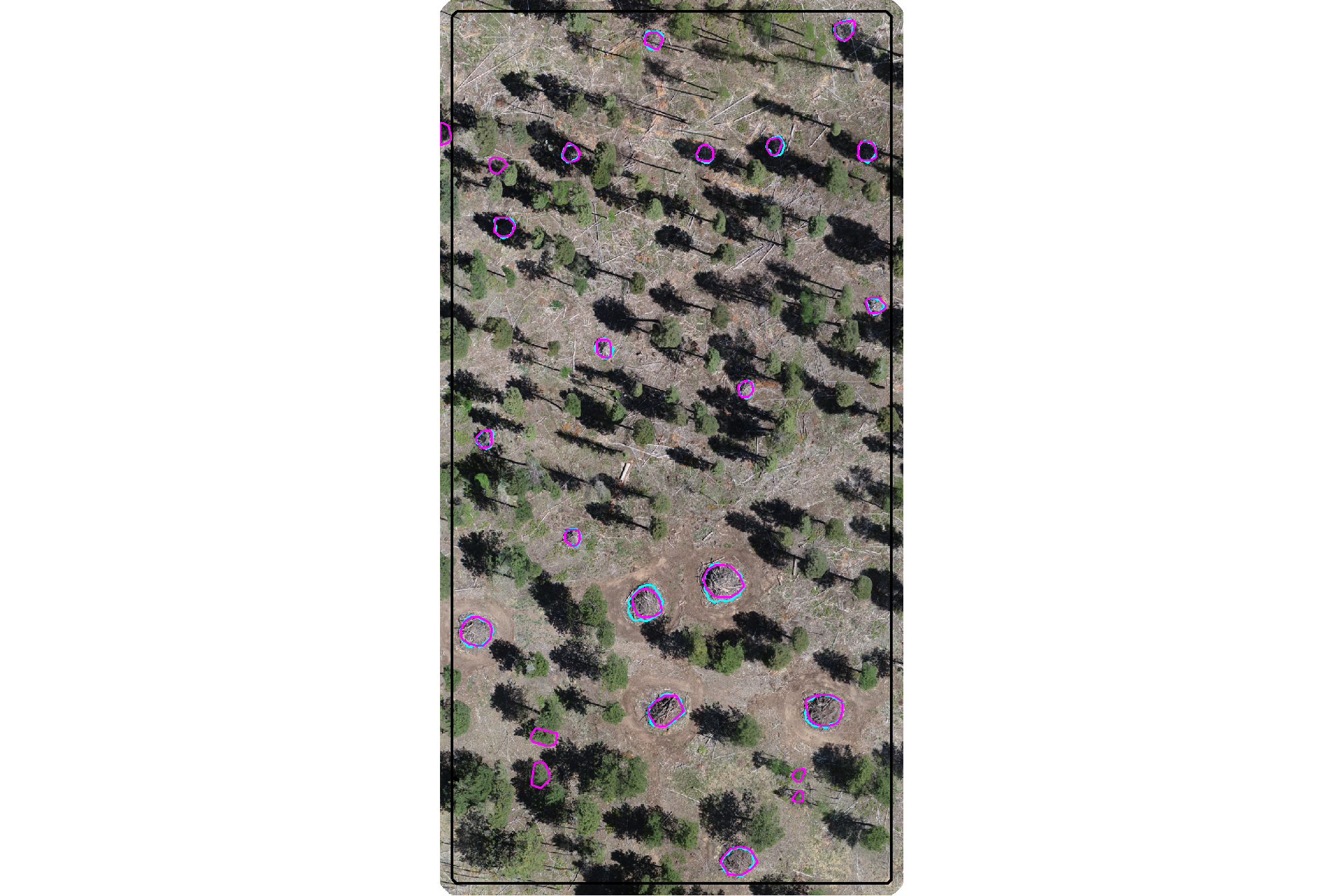
plot the filtered watershed candidate segments (magenta) and the actual piles (cyan) on the CHM
plt_aoi_chm(aoi_chm_rast_slice) +
  ggplot2::geom_sf(
    data = aoi_slash_piles_polys
    , fill = NA, color = "cyan", lwd = 0.6
  ) +
  ggplot2::geom_sf(
    data = watershed_segs_poly
    , fill = NA, color = "magenta", lwd = 0.6
  )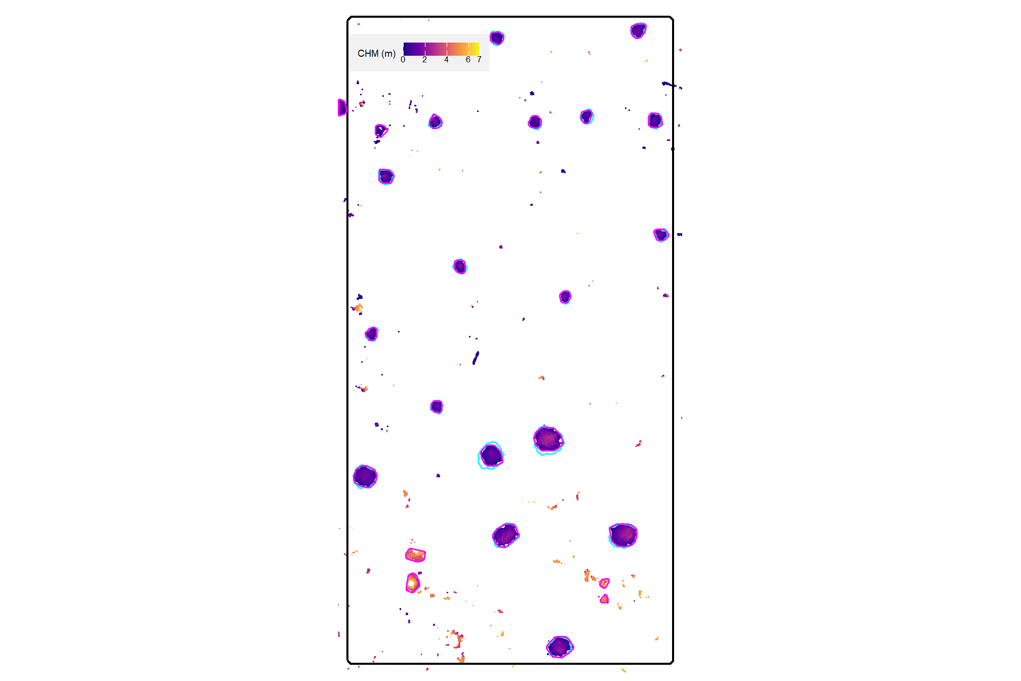
nice
4.6.2 DBSCAN Segmentation
plot the filtered dbscan candidate segments (magenta) and the actual piles (cyan) on the RGB
aoi_plt_ortho +
  ggplot2::geom_sf(data = aoi_boundary, fill = NA, color = "black", lwd = 0.8) +
  ggplot2::geom_sf(
    data = aoi_slash_piles_polys
    , fill = NA, color = "cyan", lwd = 0.6
  ) +
  ggplot2::geom_sf(
    data = dbscan_segs_poly
    , fill = NA, color = "magenta", lwd = 0.6
  ) +
  ggplot2::theme(legend.position = "none")
plot the filtered dbscan candidate segments (magenta) and the actual piles (cyan) on the CHM
plt_aoi_chm(aoi_chm_rast_slice) +
  ggplot2::geom_sf(
    data = aoi_slash_piles_polys
    , fill = NA, color = "cyan", lwd = 0.6
  ) +
  ggplot2::geom_sf(
    data = dbscan_segs_poly
    , fill = NA, color = "magenta", lwd = 0.6
  )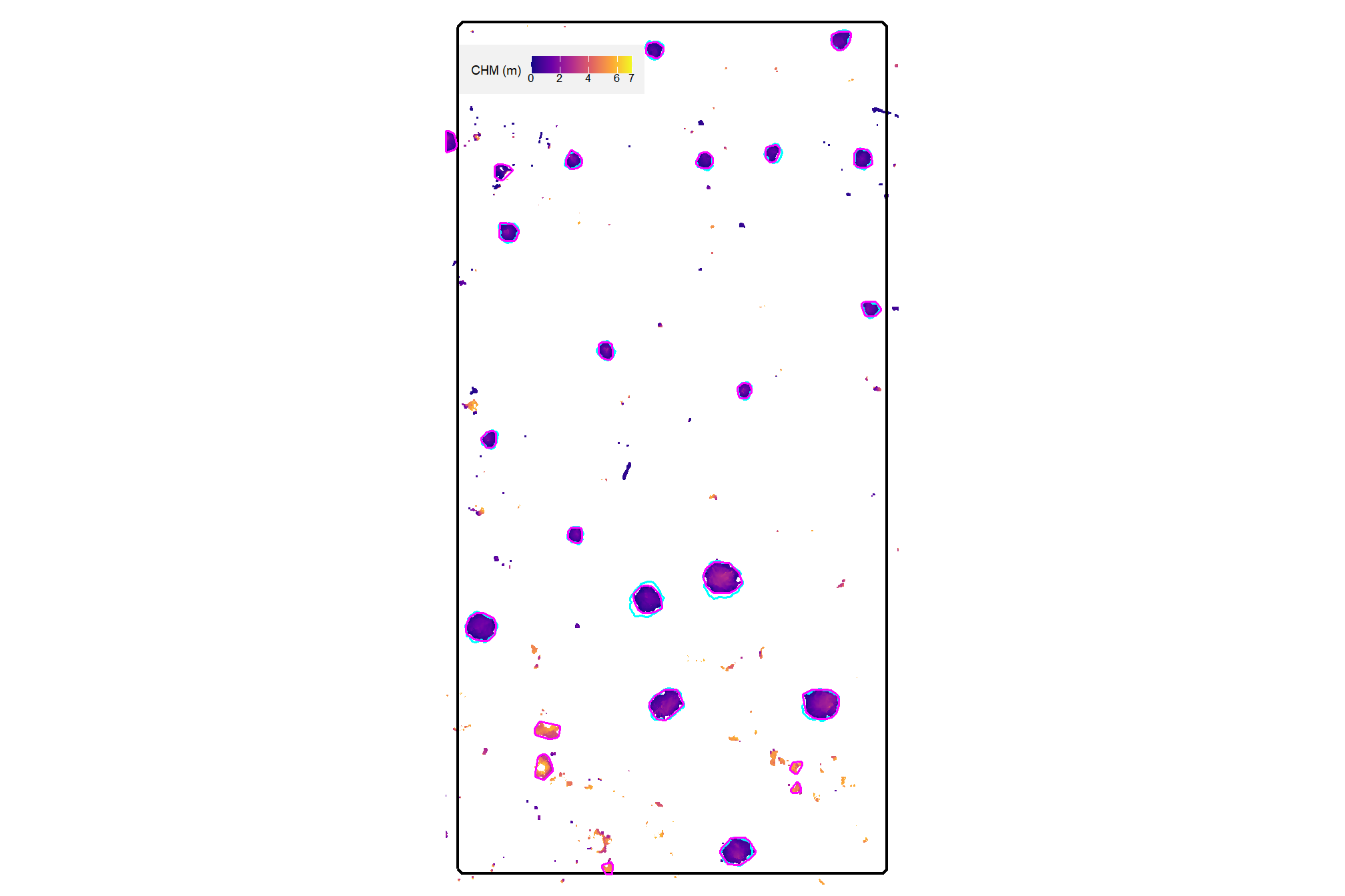
nice
4.6.3 Quick methods comparison
let’s quickly look at the watershed and dbscan segments on the same plot
ggplot2::ggplot() +
  ggplot2::geom_sf(
    data = watershed_segs_poly, mapping=ggplot2::aes(color="watershed")
    , fill = NA, lwd = 2
  ) +
  ggplot2::geom_sf(
    data = dbscan_segs_poly, mapping=ggplot2::aes(color="dbscan")
    , fill = NA, lwd = 1
  ) +
  ggplot2::scale_color_manual(values = c("gray33", "aquamarine3"),name="") +
  ggplot2::theme_void() +
  ggplot2::theme(legend.position = "top")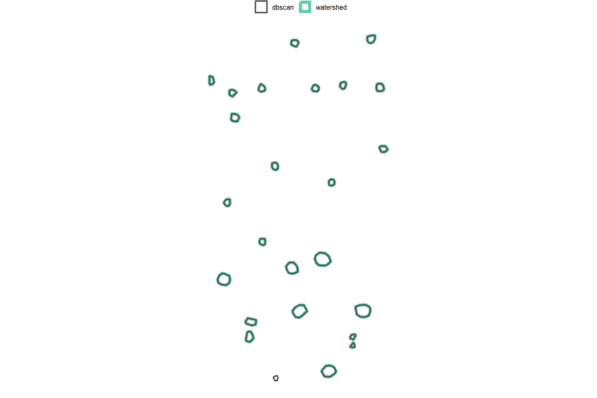
almost exactly the same
let’s see how many segments were originally detected using each method and how many we are left with after our filtering for shape irregularity, pile area and height expectations, circularity, and potential overlaps after smoothing?
dplyr::tibble(
    method = c("watershed", "DBSCAN")
    , old_segments = c(
      terra::freq(watershed_segs) %>% nrow()
      , terra::freq(dbscan_segs) %>% nrow()
    )
    , new_segments = c(
      nrow(watershed_segs_poly)
      , nrow(dbscan_segs_poly)
    )
    # area
    , old_area = c(
      terra::cellSize(watershed_segs) %>%
        terra::crop(watershed_segs,mask=T) %>%
        terra::global(fun="sum", na.rm=T) %>%
        as.numeric()
      , terra::cellSize(dbscan_segs) %>%
        terra::crop(dbscan_segs,mask=T) %>%
        terra::global(fun="sum", na.rm=T) %>%
        as.numeric()
    )
    , new_area = c(
      watershed_segs_poly %>% sf::st_union() %>% sf::st_area() %>% as.numeric()
      , dbscan_segs_poly %>% sf::st_union() %>% sf::st_area() %>% as.numeric()
    )
  ) %>%
  dplyr::mutate(
    segments_pct_removed = scales::percent((new_segments-old_segments)/old_segments, accuracy = 0.1)
    , dplyr::across(tidyselect::ends_with("segments"), ~scales::comma(.x,accuracy=1))
    , area_pct_removed = scales::percent((new_area-old_area)/old_area, accuracy = 0.1)
    , dplyr::across(tidyselect::ends_with("area"), ~scales::comma(.x,accuracy=0.1))
  ) %>%
  dplyr::select(
    method
    ,tidyselect::ends_with("_segments"), segments_pct_removed
    ,tidyselect::ends_with("_area"), area_pct_removed
  ) %>%
  kableExtra::kbl(
    caption = "Demonstration area candidate segments by method<br>final candidate segments fully filtered for size and geometric expectations"
    , col.names = c(
      "method"
      , "orig. candidate<br>segments", "final<br>segments", "% candidates<br>removed"
      , "orig. candidate<br>area (m<sup>2</sup>)", "final<br>area (m<sup>2</sup>)", "% area<br>removed"
    )
    , escape = F
  ) %>%
kableExtra::kable_styling()| method |
orig. candidate segments |
final segments |
% candidates removed |
orig. candidate area (m2) |
final area (m2) |
% area removed |
|---|---|---|---|---|---|---|
| watershed | 214 | 24 | -88.8% | 276.4 | 242.0 | -12.4% |
| DBSCAN | 200 | 25 | -87.5% | 274.4 | 245.4 | -10.6% |
wow that is a lot of filtering, but it looks like the result for this demonstration area is decently accurate (we’ll perform full validation of the method later). That is, there are few false positive predictions (commission errors) and few false negative predictions (omission errors)…in the next section we’ll integrate spectral data to further filter the false positive predictions based on how closely their spectral information matches vegetation
4.7 Pile Detection Function
The rule-based method for slash pile detection using CHM raster data we reviewed above generally follows this outline:
- CHM Generation: A Canopy Height Model (CHM) is generated from the point cloud data. The CHM is generated by removing the ground surface effectively representing a Digital Surface Model (DSM) without ground, ensuring all values are heights above bare earth.
- CHM Height Filtering: A maximum height filter is applied to the CHM to retaining only raster cells below a maximum expected slash pile height (e.g. 4 m), isolating a “slice” of the CHM.
- Segmentation Method Setup: Applies the dynamic parameter logic used in the Watershed or DBSCAN segmentation method. This logic ensures scale-invariant object detection by maintaining constant proportions between the algorithm search windows and the physical dimensions of the target object. This dynamic approach allows the method parameters to adapt automatically to the input data resolution so that the resulting candidate segments remain spatially consistent with target objects.
- Candidate Segmentation: Watershed or DBSCAN segmentation is performed on the filtered CHM raster to identify and delineate initial candidate piles based on their structural form.
- Shape Refinement & Area Filtering: To align segmentation results with real-world pile construction, we simplify candidate segments by retaining only their largest contiguous portion to eliminate detached noise and ensure each feature represents a discrete physical object. The results are then filtered based on the area expectations.
- Shape Irregularity: Convexity Filtering: Candidate pile locations are filtered to remove highly irregular shapes by assessing their overlap with their convex hull. This process removes irregular objects like branched tree crowns or segments with holes while allowing solid, regular shapes (e.g. circles, rectangles, triangles) to pass.
- Circularity Filtering: A circularity filter is applied to measure a shape’s dispersion by dividing the candidate polygon area by the area of its minimum bounding circle. This second-stage shape irregularity filter targets the round bases typical of manual construction by penalizing elongated or non-circular shapes that do not adequately fill their circumcircle.
- Final Shape Refinement & Overlap Removal: Lastly, segments are smoothed using their convex hull to remove the “blocky” raster edges (like they were made in Minecraft). Overlapping convex hull shapes are then removed to prevent false positives from clustered small trees or shrubs, ensuring singular pile detections.
Let’s package all of the steps we demonstrated when formulating the methodology into a single function which can possibly be integrated into the cloud2trees package.
The parameters are defined as follows:
min_ht_m: numeric. The minimum height (in meters) a detected pile must reach to be considered valid.max_ht_m: numeric. The maximum height (in meters) a slash pile is expected to be. This value helps us focus on a specific “slice” of the data, ignoring anything taller than a typical pile.min_area_m2: numeric. The smallest 2D area (in square meters) a detected pile must cover to be considered valid.max_area_m2: numeric. The largest 2D area (in square meters) a detected pile can cover to be considered valid.min_convexity_ratio: numeric. A value between 0 and 1 that controls how strict the filtering is for regularly shaped piles. A value of 1 means only piles that are perfectly smooth and rounded, with no dents or inward curves are kept (e.g. perfect square, rectangle, circle, triangle). A value of 0 allows for both perfectly regular and very irregular shapes. This filter works alongsidemin_circularity_ratioto identify slash piles based on expected morphology.min_circularity_ratio: numeric. A value between 0 and 1 that controls how strict the filtering is for circular pile shapes. Setting it to 1 means only piles that are perfectly circular are kept. A value of 0 allows for a wide range of shapes, including very circular and non-circular ones (like long, straight lines). For context, a perfect square has a circularity ratio of \(\frac{2}{\pi}\approx 0.637\) while an equilateral triangle has a ratio of \(\frac{3\sqrt{3}}{4\pi}\approx 0.414\). This filter works alongsidemin_convexity_ratioto identify slash piles based on expected morphology.smooth_segs: logical. Setting this option to TRUE will: 1) smooth out the “blocky” edges of detected piles (which can look like they were made in Minecraft) by using their overall shape; and 2) remove any detected piles that overlap significantly with other smoothed piles to help ensure each detection is a single slash pile, not a cluster of objects like small trees or shrubs.
# detect funciton
slash_pile_detect <- function(
  chm_rast
  , seg_method = "watershed"
  #### height and area thresholds for the detected piles
  # these should be based on data from the literature or expectations based on the prescription
  , min_ht_m # set the min expected pile height
  , max_ht_m # set the max expected pile height
  , min_area_m2 # set the min expected pile area
  , max_area_m2 # set the max expected pile area
  #### convexity filtering
  # 1 = perfectly convex (no inward angles); 0 = so many inward angles
  # values closer to 1 remove more irregular segments;
    # values closer to 0 keep more irregular segments (and also regular segments)
  # these will all be further filtered for their circularity if desired
  , min_convexity_ratio # min required overlap between the predicted pile and the convex hull of the predicted pile
  #### circularity filtering
  # 1 = perfectly circular; 0 = not circular (e.g. linear) but also circular
  # min required overlap between the candidate pile segment polygon and the minimum bounding circle of the polygon
  , min_circularity_ratio
  #### shape refinement & overlap removal
  ## smooth_segs = T ... convex hulls of raster detected segments are returned, any that overlap are removed
  ## smooth_segs = F ... raster detected segments are returned (blocky) if they meet all prior rules
  , smooth_segs = T
  ##############
  # if defined...will instead write the detected segment polygons to the file given and return the name of the file
  # ex: "my_wshed_segs.gpkg"; ex: "../data/ur_wshed_segs.gpkg"
  , ofile = NA
) {
  # checks
  if(!inherits(smooth_segs, "logical") || is.na(smooth_segs)){stop("define `smooth_segs` as logical")}
  ########################
  # shape irregularity checks
  ########################
    min_convexity_ratio <- min_convexity_ratio[1]
    min_circularity_ratio <- min_circularity_ratio[1]
    if(
      (is.na(tryCatch(as.numeric(min_convexity_ratio), error = function(e) NA)) ||
       identical(as.numeric(min_convexity_ratio), numeric(0)) ||
       !is.numeric(tryCatch(as.numeric(min_convexity_ratio), error = function(e) NA))) ||
      (is.na(tryCatch(as.numeric(min_circularity_ratio), error = function(e) NA)) ||
       identical(as.numeric(min_circularity_ratio), numeric(0)) ||
       !is.numeric(tryCatch(as.numeric(min_circularity_ratio), error = function(e) NA))) ||
      as.numeric(min_convexity_ratio)<0 ||
      as.numeric(min_convexity_ratio)>1 ||
      as.numeric(min_circularity_ratio)<0 ||
      as.numeric(min_circularity_ratio)>1
    ){
      # Code to execute if any condition is met (e.g., print an error message)
      stop("Error: One or more of `min_convexity_ratio`,`min_circularity_ratio` are not valid numbers between 0 and 1.")
    }
  ########################################################################################
  ## 1) Segmentation
  ########################################################################################
    get_segmentation_candidates_ans <- get_segmentation_candidates(
      chm_rast = chm_rast
      , method = seg_method
      , min_ht_m = min_ht_m
      , max_ht_m = max_ht_m
      , min_area_m2 = min_area_m2
      , max_area_m2 = max_area_m2
    )

    # get results individual objects
    segs_rast <- get_segmentation_candidates_ans$segs_rast
    segs_sf <- get_segmentation_candidates_ans$segs_sf
    slice_chm_rast <- get_segmentation_candidates_ans$slice_chm_rast
    # seg_mthd_params <- get_segmentation_candidates_ans$seg_mthd_params

    if(dplyr::coalesce(nrow(segs_sf),0)==0){
      stop(paste0(
        "no segments detected using the given CHM and size expectations"
        , "\n     try adjusting size threshold parameters:"
        , "\n     `min_ht_m`,`max_ht_m`,`min_area_m2`,`max_area_m2`"
      ))
    }
  ########################################################################################
  ## 2) shape refinement and area filtering
  ########################################################################################
    # to better align the segmentation results with real-world pile construction we'll now
    # simplify candidate segments composed of multiple separate parts representing a single identified feature (i.e. "multi-polygon" candidate segments.
    # We'll simplify these segments by retaining only the largest contiguous portion using `cloud2trees` functionality.
    # Because slash piles are constructed as distinct, isolated objects to prevent tree mortality during burning, this refinement step isolates the primary
    # candidate body to eliminate detached noise and ensure each segment represents a discrete physical object before area-based filtering
    segs_sf <-
      segs_sf %>%
      # simplify multipolygons by keeping only the largest portion
      dplyr::mutate(treeID = pred_id) %>%
      cloud2trees::simplify_multipolygon_crowns() %>%
      dplyr::select(-treeID) %>%
      # area filtering
      st_filter_area(min_area_m2 = min_area_m2, max_area_m2 = max_area_m2)

    if(dplyr::coalesce(nrow(segs_sf),0)==0){
      stop(paste0(
        "no segments detected using the given CHM and size expectations"
        , "\n     try adjusting size threshold parameters:"
        , "\n     `min_area_m2`,`max_area_m2`"
      ))
    }

  ########################################################################################
  ## 3) convexity filtering
  ########################################################################################
    # let's first filter out segments that have holes in them
    # or are very irregularly shaped by comparing the area of the polygon and convex hull
    # min_convexity_ratio = min required overlap between the predicted pile and the convex hull of the predicted pile
    if(min_convexity_ratio>0){
      # apply the convexity filtering on the polygons
      segs_sf <- st_convexity_filter(
          sf_data = segs_sf
          # min required overlap between the polygon and the convex hull of the polygon
          , min_convexity_ratio = min_convexity_ratio
        )
    }

    # check return
    if(dplyr::coalesce(nrow(segs_sf),0)==0){
      stop(paste0(
        "no segments detected using the given CHM and `min_convexity_ratio` expectations"
        , "\n     try adjusting `min_convexity_ratio` "
      ))
    }

  ########################################################################################
  ## 4) circularity filtering
  ########################################################################################
    # let's apply a minimum bounding circle algorithm to remove non-circular segments from the remaining segments
    if(min_circularity_ratio>0){
      # apply the circularity filtering on the polygons
      segs_sf <- st_circularity_filter(
          sf_data = segs_sf
          # min required overlap between the polygon and the minimum bounding circle of the polygon
          , min_circularity_ratio = min_circularity_ratio
        )
    }

    # check return
    if(dplyr::coalesce(nrow(segs_sf),0)==0){
      stop(paste0(
        "no segments detected using the given CHM and `min_circularity_ratio` expectations"
        , "\n     try adjusting `min_circularity_ratio` "
      ))
    }

  ########################################################################################
  ## 5) calculate CHM-based structural metrics for the candidate piles
  ########################################################################################
    # we'll use our `get_structural_metrics()` with the height-filtered CHM to compute the structural metrics for the candidate piles
    segs_sf <-
      get_structural_metrics(
        sf_data = segs_sf
        , chm_rast = slice_chm_rast
      ) %>%
      purrr::pluck("sf_data") %>%
      # we may already have area so we'll use only the value from this function
      dplyr::select( -dplyr::any_of(c(
        "hey_xxxxxxxxxx"
        , "poly_area_m2"
      )))

    # check return
    if(dplyr::coalesce(nrow(segs_sf),0)==0){
      stop(paste0(
        "trouble getting the structural metrics"
        , "\n     try adjusting .... something "
      ))
    }

    # filter for height
    segs_sf <- segs_sf %>%
      dplyr::filter(
        max_height_m >= min_ht_m
        & max_height_m <= max_ht_m
      )

    # check return
    if(dplyr::coalesce(nrow(segs_sf),0)==0){
      stop(paste0(
        "no segments detected using the given CHM and size expectations"
        , "\n     try adjusting size threshold parameters:"
        , "\n     `min_ht_m`,`max_ht_m`"
      ))
    }

  ########################################################################################
  ## 6) shape refinement & overlap removal
  ########################################################################################
    # use the convex hull shapes of our remaining segments.
    # This helps to smooth out the often 'blocky' edges of raster-based segments
    # , which can look like they were generated in Minecraft.
    # Additionally, by removing any segments with overlapping convex hull shapes,
    # we can likely reduce false detections that are actually groups of small trees or shrubs,
    # ensuring our results represent singular slash piles.

    if(smooth_segs){
      # take the convex hull and apply our `st_remove_overlaps()` function to the remaining candidate segments.
      # Finally, we filter for area based on the smoothed shape
      segs_sf <-
        segs_sf %>%
        sf::st_convex_hull() %>%
        sf::st_simplify() %>%
        sf::st_make_valid() %>%
        dplyr::filter(sf::st_is_valid(.)) %>%
        st_remove_overlaps() %>%
        # now we need to re-do the volume and area calculations
        dplyr::mutate(
          area_m2 = sf::st_area(.) %>% as.numeric()
          , volume_m3 = area_m2*volume_per_area
        ) %>%
        st_filter_area(min_area_m2 = min_area_m2, max_area_m2 = max_area_m2)

      # check return
      if(dplyr::coalesce(nrow(segs_sf),0)==0){
        stop(paste0(
          "no segments detected after removing overlapping final segments"
          , "\n     try with `smooth_segs = F`"
        ))
      }
    }

    # calculate diameter
    segs_sf <- st_calculate_diameter(segs_sf)

  # check for write
    if(
      inherits(ofile,"character")
      && stringr::str_squish(ofile)!=""
      && !identical(stringr::str_squish(ofile),character(0))
    ){
      sf::st_write(segs_sf, dsn = ofile, quiet = T, append = F)
      return(ofile)
    }

  # return
    return(list(
      segs_sf = segs_sf
      , seg_mthd_params = get_segmentation_candidates_ans$seg_mthd_params
      , slice_chm_rast = get_segmentation_candidates_ans$slice_chm_rast
    ))
}
remove all other parameters and objects that might have the same name as in this function since we used the framework outlined above to define this (fantastic?) beast of a function
remove(
  min_ht_m, max_ht_m
  , min_area_m2, max_area_m2
  , min_convexity_ratio
  , min_circularity_ratio
  , get_segmentation_params_ans
  , dbscan_segs_poly, watershed_segs_poly
  , dbscan_segs, watershed_segs
  , dbscan_segs_poly_chull, dbscan_segs_poly_mbc
  , watershed_segs_poly_chull, watershed_segs_poly_mbc
  , aoi_chm_rast_slice
)
gc()
let’s test this real quick on our example area
slash_pile_detect_watershed_ans_temp <- slash_pile_detect(
  chm_rast = aoi_chm_rast
  , seg_method = "watershed"
  , min_ht_m = 1
  , max_ht_m = 4
  , min_area_m2 = 1.5^2
  , max_area_m2 = 50
  , min_convexity_ratio = 0.7
  , min_circularity_ratio = 0.5
)
the slash_pile_detect() function returns:
segs_sf: the segments that passed all size and geometric expectations for target slash pilesseg_mthd_params: the dynamic parameters used in the Watershed or DBSCAN segmentation methodslice_chm_rast: the height-filtered CHM slice used to segment candidate slash piles
## List of 3
##  $ segs_sf        : sf [19 × 9] (S3: sf/tbl_df/tbl/data.frame)
##   ..$ pred_id          : num [1:19] 54 69 83 84 87 88 89 94 100 101 ...
##   ..$ convexity_ratio  : num [1:19] 0.91 0.894 0.93 0.881 0.933 ...
##   ..$ circularity_ratio: num [1:19] 0.697 0.671 0.754 0.652 0.662 ...
##   ..$ area_m2          : num [1:19] 25.32 26.82 5.05 20.26 6.18 ...
##   ..$ volume_m3        : num [1:19] 34.55 39.72 4.39 21.23 4.48 ...
##   ..$ max_height_m     : num [1:19] 3.57 3.18 2.56 2.54 2.36 ...
##   ..$ volume_per_area  : num [1:19] 1.364 1.481 0.868 1.048 0.725 ...
##   ..$ geometry         :sfc_POLYGON of length 19; first list element: List of 1
##   .. ..- attr(*, "class")= chr [1:3] "XY" "POLYGON" "sfg"
##   ..$ diameter_m       : num [1:19] 6.45 6.75 2.82 5.91 3.33 ...
##   ..- attr(*, "sf_column")= chr "geometry"
##   ..- attr(*, "agr")= Factor w/ 3 levels "constant","aggregate",..: NA NA NA NA NA NA NA NA
##   .. ..- attr(*, "names")= chr [1:8] "pred_id" "convexity_ratio" "circularity_ratio" "area_m2" ...
##  $ seg_mthd_params:List of 3
##   ..$ data_summary:List of 2
##   .. ..$ pts_per_m2: num 100
##   .. ..$ rast_res_m: num 0.1
##   ..$ watershed   :List of 2
##   .. ..$ tol: num 1.5
##   .. ..$ ext: num 2
##   ..$ dbscan      :List of 2
##   .. ..$ eps   : num 0.15
##   .. ..$ minPts: num 7
##  $ slice_chm_rast :S4 class 'SpatRaster' [package "terra"]
let’s check out the height-filtered CHM “slice”
slash_pile_detect_watershed_ans_temp$slice_chm_rast %>%
  terra::plot(axes = F, col = viridis::plasma(100), main = "filtered CHM (m)")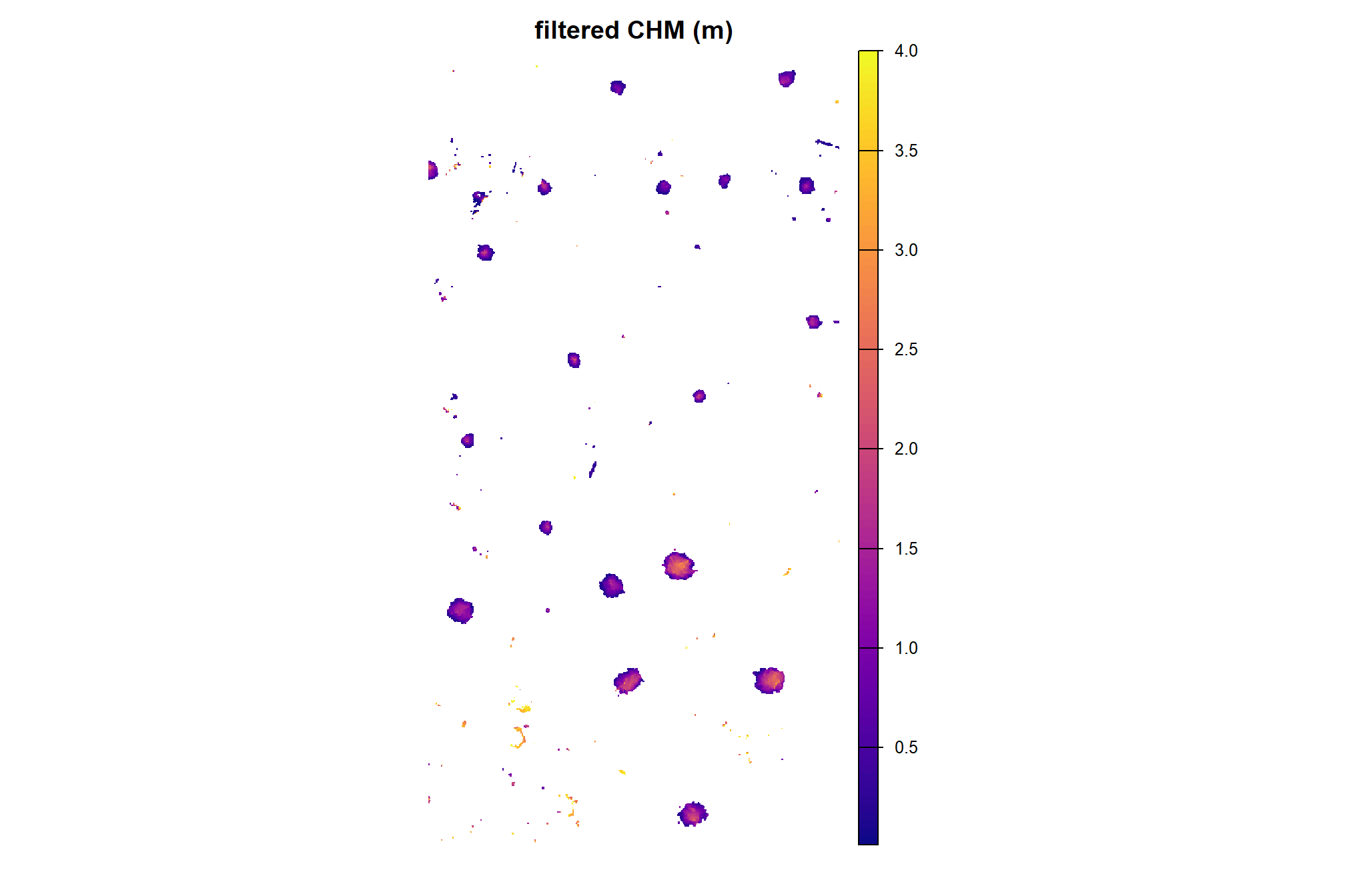
let’s overlay the final candidate segments (magenta) and the actual piles (cyan) on the raw, un-filtered CHM
aoi_chm_rast %>%
  terra::plot(axes = F, col = viridis::plasma(100), main = "CHM (m) and demonstration piles")
terra::plot(
  aoi_slash_piles_polys %>%
    sf::st_transform(terra::crs(aoi_chm_rast)) %>%
    terra::vect()
  , add = T, border = "cyan", col = NA, lwd = 2
)
terra::plot(
  slash_pile_detect_watershed_ans_temp$segs_sf %>% terra::vect()
  , add = T, border = "magenta", col = NA, lwd = 2.5
)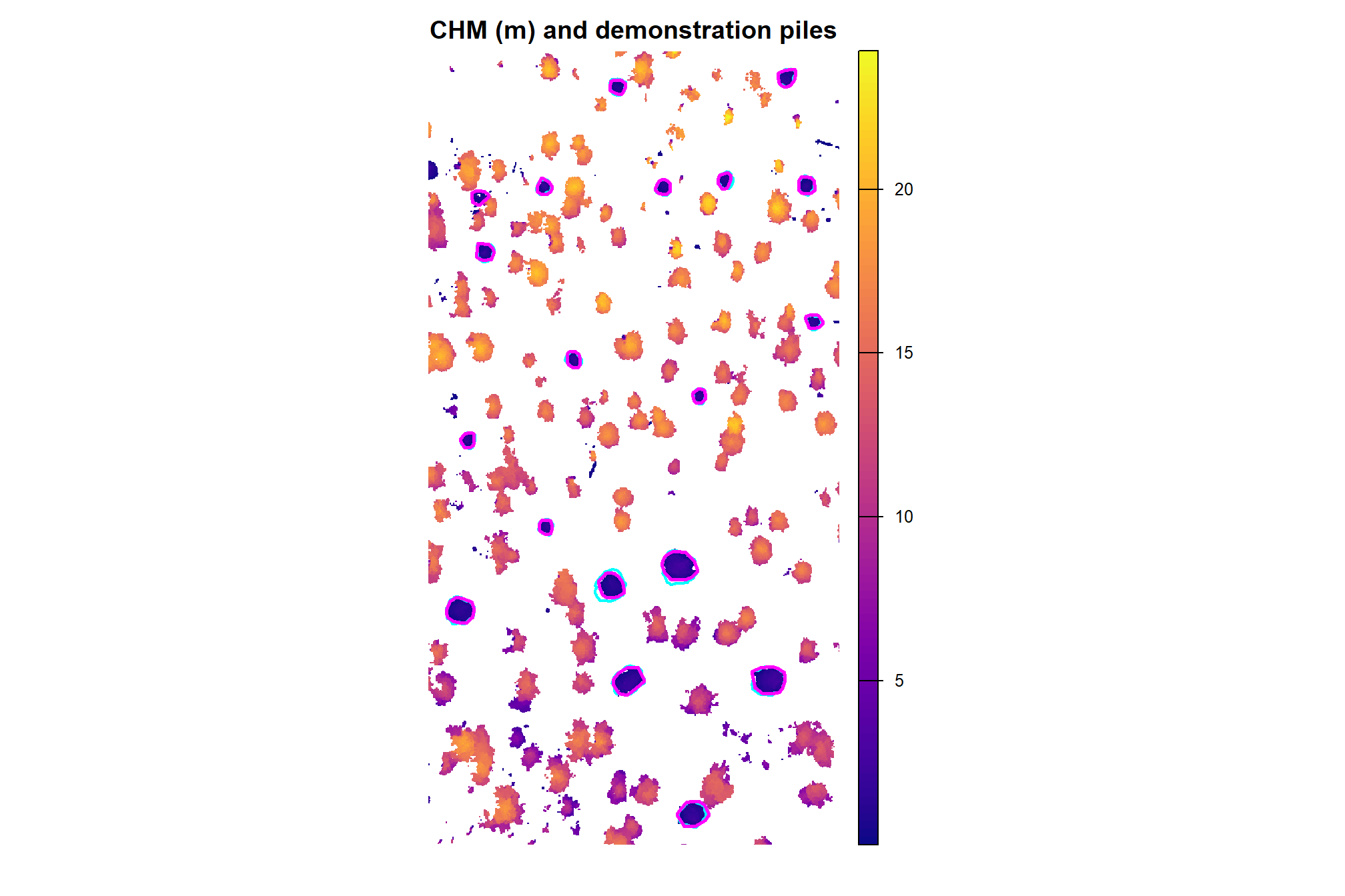
how do the form quantification measurements look?
p1_temp <- slash_pile_detect_watershed_ans_temp$segs_sf %>%
  ggplot2::ggplot() +
  ggplot2::geom_sf(mapping = ggplot2::aes(fill = area_m2)) +
  ggplot2::scale_fill_distiller(palette = "Blues", direction = 1) +
  ggplot2::labs(x="",y="", fill = "", subtitle = "area_m2") +
  ggplot2::theme_light() +
  ggplot2::theme(legend.position = "top", axis.text = ggplot2::element_blank(), plot.subtitle = ggplot2::element_text(size = 7,hjust=0.5))
p2_temp <- slash_pile_detect_watershed_ans_temp$segs_sf %>%
  ggplot2::ggplot() +
  ggplot2::geom_sf(mapping = ggplot2::aes(fill = volume_m3)) +
  ggplot2::scale_fill_distiller(palette = "Purples", direction = 1) +
  ggplot2::labs(x="",y="", fill = "", subtitle = "volume_m3") +
  ggplot2::theme_light() +
  ggplot2::theme(legend.position = "top", axis.text = ggplot2::element_blank(), plot.subtitle = ggplot2::element_text(size = 7,hjust=0.5))
p3_temp <- slash_pile_detect_watershed_ans_temp$segs_sf %>%
  ggplot2::ggplot() +
  ggplot2::geom_sf(mapping = ggplot2::aes(fill = max_height_m)) +
  ggplot2::scale_fill_distiller(palette = "Greens", direction = 1) +
  ggplot2::labs(x="",y="", fill = "", subtitle = "max_height_m") +
  ggplot2::theme_light() +
  ggplot2::theme(legend.position = "top", axis.text = ggplot2::element_blank(), plot.subtitle = ggplot2::element_text(size = 7,hjust=0.5))
p4_temp <- slash_pile_detect_watershed_ans_temp$segs_sf %>%
  ggplot2::ggplot() +
  ggplot2::geom_sf(mapping = ggplot2::aes(fill = diameter_m)) +
  ggplot2::scale_fill_distiller(palette = "PuRd", direction = 1) +
  ggplot2::labs(x="",y="", fill = "", subtitle = "diameter_m") +
  ggplot2::theme_light() +
  ggplot2::theme(legend.position = "top", axis.text = ggplot2::element_blank(), plot.subtitle = ggplot2::element_text(size = 7,hjust=0.5))
(p1_temp + p2_temp) / (p3_temp + p4_temp)