Section 2 Data Overview

We will detail the study sites and summarize the number of piles and the pile size based on available measurements.

Site Name	Pile Type	Validation Data Type	Unique Features & Ecology	Data Collection (UAS Platform & Parameters)
PSINF Mixed Conifer Site	Hand Piles and smaller machine piles	Image-annotated footprints and field-measured height and diameter	Located in the Pike and San Isabel National Forest (PSINF) in CO, US. Mixed conifer stand with variable ground cover and canopy density.	Switchblade-Elite (Vision Aerial) with 24.2 MP RGB sensor (16 mm lens). Altitude xx m, 90% forward and 85% side overlap, 4 m/s speed.
TRFO-BLM Pinyon-Juniper Site	Hand Piles	Image-annotated footprints based on field collected point locations	Located on BLM land in CO, US. Arid environment with dry vegetation including standing dead pinyon-juniper. Piles are smaller, simpler, and hand-stacked.	Freefly Astro with Sony ILX-LR1 (35mm lens). Altitude 243.84 m (terrain following), 85% forward and 80% side overlap.
BHEF Ponderosa Pine Site	Machine Piles	Image-annotated footprints	Located in the Black Hills Experimental Forest (BHEF) in SD, US. Piles are massive, mechanically built, and irregularly shaped (e.g. not necessarily circular). Tree regeneration is expected.	DJI Phantom 4 Pro with 20 MP RGB sensor (8.8 mm lens). Altitude 80 m, 90% forward and 85% side overlap, 4 m/s speed.
ARNF Ponderosa Pine Site	Machine Piles	Image-annotated footprints	Located in the Arapahoe and Roosevelt National Forest (ARNF) in CO, US. Ponderosa pine forest with a climate similar to PSINF. Machine piles are massive but more circular and regular. Less regeneration is expected.	Switchblade-Elite (Vision Aerial) with 24.2 MP RGB sensor (16 mm lens). Altitude xx m, 90% forward and 85% side overlap, 4 m/s speed.

Load the standard libraries we use to do work

# bread-and-butter
library(tidyverse) # the tidyverse
library(viridis) # viridis colors
library(harrypotter) # hp colors
library(RColorBrewer) # brewer colors
library(scales) # work with number and plot scales
library(latex2exp)

# visualization
library(mapview) # interactive html maps
library(kableExtra) # tables
library(patchwork) # combine plots
library(ggnewscale) # new scale
library(ggrepel) # repel labels
library(grDevices) # default graphics

# spatial analysis
library(terra) # raster
library(sf) # simple features
library(lwgeom) # advanced functions for spatial operations
library(lidR) # lidar data
library(rgl) # 3d plots
library(cloud2trees) # the cloud2trees

# statistical analysis
library(brms) # brms
library(tidybayes) # tidybayes

2.1 Study Units Vector Data

let’s load in all the vector data containing the study units

we’ll combine the study unit boundaries for all sites to create a spatial data set that contains all units for plotting in a single map

# read the data
# stand boundary
all_stand_boundary <-
  dplyr::bind_rows(
    psinf_stand_boundary %>% 
      sf::st_transform(crs = 5070) %>% 
      dplyr::select(site) %>% 
      sf::st_set_geometry("geometry")
    , pj_stand_boundary %>% 
      sf::st_transform(crs = 5070) %>% 
      dplyr::select(site) %>% 
      sf::st_set_geometry("geometry")
    , bhef_stand_boundary %>% 
      sf::st_transform(crs = 5070) %>% 
      dplyr::select(site) %>% 
      sf::st_set_geometry("geometry")
    , arnf_stand_boundary %>% 
      sf::st_transform(crs = 5070) %>% 
      dplyr::select(site) %>% 
      sf::st_set_geometry("geometry")
  ) %>% 
  dplyr::group_by(site) %>% 
  dplyr::summarise(
    geometry = sf::st_union(geometry)
  ) %>% 
  dplyr::ungroup() %>% 
  sf::st_set_geometry("geometry") %>% 
  dplyr::mutate(
    site_area_m2 = sf::st_area(geometry) %>% as.numeric()
    , site_area_ha = site_area_m2/10000
    , site_data_lab = dplyr::case_match(
      site
      , "PSINF Mixed Conifer Site" ~ "psinf"
      , "TRFO-BLM Pinyon-Juniper Site" ~ "pj"
      , "BHEF Ponderosa Pine Site" ~ "bhef"
      , "ARNF Ponderosa Pine Site" ~ "arnf"
    )
    , site_full_lab = dplyr::case_match(
      site
      , "PSINF Mixed Conifer Site" ~ "Pike and San Isabel National Forest (PSINF)"
      , "TRFO-BLM Pinyon-Juniper Site" ~ "Tres Rios Field Office (TRFO-BLM)"
      , "BHEF Ponderosa Pine Site" ~ "Black Hills Experimental Forest (BHEF)"
      , "ARNF Ponderosa Pine Site" ~ "Arapahoe and Roosevelt National Forest (ARNF)"
    )
  )
  # sf::st_centroid() %>% 
  # sf::st_sf() %>% 

Let’s map the study sites on a single map

sites_pal <- RColorBrewer::brewer.pal(n = nrow(all_stand_boundary), name = "Dark2")
# option to put satellite imagery as base layer of mapview maps
mapview::mapviewOptions(
  homebutton = T
  # , basemaps = c("Esri.WorldImagery","OpenStreetMap")
  , basemaps = c("OpenStreetMap", "Esri.WorldImagery")
)
# map it
mapview::mapview(
  all_stand_boundary %>% 
    dplyr::group_by(site) %>% 
    sf::st_centroid()
  , zcol="site"
  , col.regions = sites_pal
  , cex = 8
  , layer.name = "study sites"
)

static map for printing

let’s make a pretty image for use in the journal article. we’ll use the ggmap package to get a nice background map and do some transformation to actually work with the map. We’ll add a map scale using ggspatial

library(ggmap)
library(ggspatial)
#########################################################################
#########################################################################
# Make each plot individually by landscape as solution to small multiples
# this block defines function
#########################################################################
##################hack to align plots for ggmap
ggmap_bbox_fn <- function(map, my_crs=3857) {
    if (!inherits(map, "ggmap")) stop("map must be a ggmap object")
    # Extract the bounding box (in lat/lon) from the ggmap to a numeric vector, 
    # and set the names to what sf::st_bbox expects:
    map_bbox <- setNames(unlist(attr(map, "bb")), c("ymin", "xmin", "ymax", "xmax"))
    # Convert the bbox to an sf polygon, transform it to 3857, 
    # and convert back to a bbox (convoluted, but it works)
    bbox_3857 <- st_bbox(st_transform(st_as_sfc(st_bbox(map_bbox, crs = 4326)), my_crs))
    # Overwrite the bbox of the ggmap object with the transformed coordinates 
    attr(map, "bb")$ll.lat <- bbox_3857["ymin"]
    attr(map, "bb")$ll.lon <- bbox_3857["xmin"]
    attr(map, "bb")$ur.lat <- bbox_3857["ymax"]
    attr(map, "bb")$ur.lon <- bbox_3857["xmax"]
    map
}
plt_crs <- 3857
#########################################################################
#########################################################################
#########################################################################
my_ggmap_basemap <- function(sf_data, zoom_level = 14, buffer_box = 2600, my_crs = plt_crs, scale_location = "bl", my_maptype = "stamen_terrain") {
  
  # # should zoom in?
  # zoom_level <- 14 # 11
  # # should buffer extend?
  # buffer_box <- 2600 # 20000
  # bounding box
  bb_temp <-
    sf_data %>% 
    sf::st_bbox() %>% 
    sf::st_as_sfc() %>% 
    sf::st_transform(crs=5070) %>% 
    sf::st_buffer(as.numeric(buffer_box)) %>% 
    sf::st_transform(crs=4326) %>% # same as get_map return
    sf::st_bbox()
  # set bbox for get call
  bbox_temp <- c(
    bottom = bb_temp[[2]]
    , top = bb_temp[[4]]
    , right = bb_temp[[3]]
    , left = bb_temp[[1]]
  )
  hey_ggmap <- ggmap::get_stadiamap(
    bbox = bbox_temp
    , zoom = zoom_level
    , maptype = my_maptype #"stamen_terrain" #"stamen_toner_lite"
    , crop = T
  )

  # ggmap::ggmap(hey_ggmap)
  # apply align function
  hey_ggmap_aligned <- ggmap_bbox_fn(hey_ggmap, my_crs) # Use the function
  # plot
  plt_basemap <-
    ggmap::ggmap(hey_ggmap_aligned) + 
    ggplot2::coord_sf(
      expand = FALSE
    ) +
    ggplot2::theme_light() +
    ggplot2::theme(
      legend.position = "none"
      , plot.title = ggplot2::element_blank()
      , strip.text = ggplot2::element_blank()
      , axis.title = ggplot2::element_blank()
      , axis.text = ggplot2::element_blank()
      , axis.ticks = ggplot2::element_blank()
      , panel.grid = ggplot2::element_blank()
      , plot.margin = ggplot2::margin(0, 0, 0, 0, "cm")
    )
  if(scale_location %in% c("bl", "br", "tr", "tl")){
    plt_basemap <- plt_basemap + 
      ggspatial::annotation_scale(
        location = scale_location
        , style = "ticks"
        , pad_x = unit(0.1, "cm")
        , pad_y = unit(0.1, "cm")
      )
  }
  return(plt_basemap)
}

plot the fancy basemap with the points

# get the basemap with our my_ggmap_basemap()
plt_basemap <- my_ggmap_basemap(
  sf_data = all_stand_boundary %>% dplyr::group_by(site) %>% sf::st_point_on_surface()
  , buffer_box = 130000 # 190000
  , zoom_level = 7
  , my_maptype = "stamen_terrain"
  , scale_location = "br"
)
# plt_basemap
# plot
plt1_temp <- 
  plt_basemap + 
    ggplot2::geom_sf(
      data = all_stand_boundary %>% 
        dplyr::group_by(site_full_lab) %>% 
        sf::st_point_on_surface() %>% 
        sf::st_transform(crs=plt_crs)
      , mapping = ggplot2::aes(fill = site_full_lab)
      , size = 5
      , inherit.aes = F
      , shape = 21
      , color = "gray88"
      , fill = "blue2"
    )
plt2_temp <- plt1_temp +
    ggplot2::geom_sf_label(
      data = all_stand_boundary %>% 
        dplyr::group_by(site_full_lab) %>% 
        sf::st_point_on_surface() %>% 
        sf::st_transform(crs=plt_crs)
      , mapping = ggplot2::aes(label = stringr::str_wrap(site_full_lab, width = 25))
      , size = 2.8
      , hjust = -0.06
      , vjust = -0.1 # 0.5
      , inherit.aes = F
      , label.padding = ggplot2::unit(0.4, "lines")
    ) +
    ggplot2::scale_fill_manual(values = sites_pal)
plt2_temp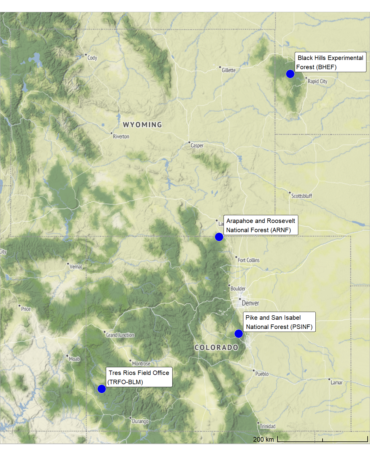

what is the area of the treatment unit boundaries we are looking over?

all_stand_boundary %>% 
  sf::st_drop_geometry() %>% 
  dplyr::select(site, site_area_ha) %>% 
  dplyr::mutate(
    site_area_ha = scales::comma(site_area_ha, suffix = " ha", accuracy = 0.1)
  ) %>% 
  kableExtra::kbl(
    caption = "Study site area"
    , col.names = c(
      "site", "hectares"
    )
    , escape = F
  ) %>% 
  kableExtra::kable_styling()

Table 2.1: Study site area

site	hectares
ARNF Ponderosa Pine Site	73.6 ha
BHEF Ponderosa Pine Site	103.1 ha
PSINF Mixed Conifer Site	17.5 ha
TRFO-BLM Pinyon-Juniper Site	5.2 ha

2.2 Slash Pile Vector Data

Image-annotated pile footprints at each study site were created in a GIS by outlining pile boundaries on the RGB orthomosaic and confirming the vertical structure using fine-resolution CHM data (e.g., 0.15m resolution). Field-collected points were used to ensure pile census completeness at the hand-pile study sites (PSINF Mixed Conifer Site and TRFO-BLM Pinyon-Juniper Site) to pinpoint piles that were otherwise challenging to delineate from the aerial imagery and CHM data alone. Across all sites, machine piles were easily distinguishable using the RGB and CHM data.

Let’s load in those image-annotated pile polygons now for each study site.

#######################################
# polygons annotated using RGB and field-collected points
#######################################
###########################
# PSINF Mixed Conifer Site
###########################
  psinf_slash_piles_polys <- sf::st_read(
      "../data/PFDP_Data/PFDP_SlashPiles/manitou_pile_polys.shp"
      , quiet = T
    ) %>% 
    dplyr::rename_with(tolower) %>% 
    sf::st_make_valid() %>% 
    dplyr::filter(sf::st_is_valid(.)) %>% 
    # fix multipolygons
    dplyr::ungroup() %>% 
    dplyr::mutate(treeID = dplyr::row_number()) %>% 
    cloud2trees::simplify_multipolygon_crowns() %>% 
    dplyr::select(-c(treeID, shape_leng, shape_area)) %>% 
    dplyr::mutate(site = "PSINF Mixed Conifer Site")
  
  # points recorded in field
  psinf_slash_piles_points <- sf::st_read(
      "../data/PFDP_Data/PFDP_SlashPiles/SlashPiles.shp"
      , quiet = T
    ) %>% 
    dplyr::rename_with(tolower) %>% 
    sf::st_zm() %>% 
    sf::st_transform(sf::st_crs(psinf_slash_piles_polys)) %>% 
    dplyr::filter( !(objectid %in% c(43)) ) %>% # duplicate field points
    dplyr::mutate(row_number = dplyr::row_number()) %>% 
    dplyr::select(-c(objectid)) %>% 
    dplyr::rename(
      height_ft = height
      , diameter_ft = diameter
    )
  # update unit boundary to pile proj
  psinf_stand_boundary <- psinf_stand_boundary %>% sf::st_transform(sf::st_crs(psinf_slash_piles_polys))
  
  # attach flag for spatial overlap with unit boundary
  psinf_slash_piles_polys <- psinf_slash_piles_polys %>%
    dplyr::left_join(
      psinf_slash_piles_polys %>% 
        sf::st_intersection(psinf_stand_boundary) %>% 
        sf::st_drop_geometry() %>% 
        dplyr::select(pile_id) %>% 
        dplyr::mutate(is_in_stand = T)
      , by = "pile_id"
    ) %>% 
    dplyr::mutate(
      is_in_stand = dplyr::coalesce(is_in_stand, F)
    )
###########################
# TRFO-BLM Pinyon-Juniper Site
###########################
  pj_slash_piles_polys <- 
    sf::st_read("../data/Dawson_Data/piles/pj_pile_polys.shp", quiet=T) %>% 
    dplyr::rename_with(tolower) %>% 
    sf::st_make_valid() %>% 
    dplyr::filter(sf::st_is_valid(.)) %>% 
    # fix multipolygons
    dplyr::mutate(
      pile_id = dplyr::row_number()
      , treeID = dplyr::row_number()
    ) %>% 
    cloud2trees::simplify_multipolygon_crowns() %>%
    dplyr::select(-c(treeID,id)) %>% 
    dplyr::filter(pile_id!=62) %>% 
    dplyr::mutate(site = "TRFO-BLM Pinyon-Juniper Site")
  
  # points recorded in field
  # these piles were collected twice in the same location and have different measurements :\
  bad_pile_ids_temp <- c(
    142
    , 146
    , 99
    , 96
    , 50
    , 268
  )
  pj_slash_piles_points <- 
    readr::read_csv("../data/Dawson_data/PJ_Piles_Unit_10.csv", progress = T, show_col_types = F) %>% 
    dplyr::rename_with(tolower) %>% 
    dplyr::rename_with(stringr::str_squish) %>% 
    dplyr::rename_with(make.names) %>% 
    dplyr::rename_with(~stringr::str_replace_all(.x, "\\.{2,}", ".")) %>% 
    dplyr::rename_with(~stringr::str_remove(.x, "\\.$")) %>% 
    dplyr::rename_with(~stringr::str_replace_all(.x, "\\.", "_")) %>% 
    dplyr::mutate(
      orig_pile_id = readr::parse_number(name)
    ) %>% 
    dplyr::filter(
      !(orig_pile_id %in% bad_pile_ids_temp)
    ) %>% 
    sf::st_as_sf(coords = c("easting","northing"), crs = 6342, remove = F) %>% 
    dplyr::select(orig_pile_id,name,height_m,width_m,easting,northing,latitude,longitude,code,description,elevation) %>% 
    sf::st_make_valid() %>% 
    sf::st_transform(sf::st_crs(pj_slash_piles_polys))
  
  # update unit boundary to pile proj
  pj_stand_boundary <- pj_stand_boundary %>% sf::st_transform(sf::st_crs(pj_slash_piles_polys))
  
  # attach flag for spatial overlap with unit boundary
  pj_slash_piles_polys <- pj_slash_piles_polys %>%
    dplyr::left_join(
      pj_slash_piles_polys %>% 
        sf::st_intersection(pj_stand_boundary) %>% 
        sf::st_drop_geometry() %>% 
        dplyr::select(pile_id) %>% 
        dplyr::mutate(is_in_stand = T)
      , by = "pile_id"
    ) %>% 
    dplyr::mutate(
      is_in_stand = dplyr::coalesce(is_in_stand, F)
    )
###########################  
# BHEF Ponderosa Pine Site
###########################  
  bhef_slash_piles_polys <- 
    sf::st_read("../data/BHEF_202306/piles/bhef_pile_polys.shp", quiet=T) %>% 
    dplyr::rename_with(tolower) %>% 
    sf::st_make_valid() %>% 
    dplyr::filter(sf::st_is_valid(.)) %>% 
    # fix multipolygons
    dplyr::mutate(
      pile_id = dplyr::row_number()
      , treeID = dplyr::row_number()
    ) %>% 
    cloud2trees::simplify_multipolygon_crowns() %>%
    dplyr::select(-c(treeID)) %>% 
    dplyr::mutate(site = "BHEF Ponderosa Pine Site")
  
  # update unit boundary to pile proj
  bhef_stand_boundary <- bhef_stand_boundary %>% sf::st_transform(sf::st_crs(bhef_slash_piles_polys))
  
  # attach flag for spatial overlap with unit boundary
  bhef_slash_piles_polys <- bhef_slash_piles_polys %>%
    dplyr::left_join(
      bhef_slash_piles_polys %>% 
        sf::st_intersection(bhef_stand_boundary) %>% 
        sf::st_drop_geometry() %>% 
        dplyr::select(pile_id) %>% 
        dplyr::mutate(is_in_stand = T)
      , by = "pile_id"
    ) %>% 
    dplyr::mutate(
      is_in_stand = dplyr::coalesce(is_in_stand, F)
    )
###########################  
# ARNF Ponderosa Pine Site
###########################  
  arnf_slash_piles_polys <- 
    sf::st_read("../data/ARNF_DiamondView_202510/arnf_diamond_view_pile_polys.shp", quiet=T) %>% 
    dplyr::rename_with(tolower) %>% 
    sf::st_make_valid() %>% 
    dplyr::filter(sf::st_is_valid(.)) %>% 
    # fix multipolygons
    dplyr::mutate(
      pile_id = dplyr::row_number()
      , treeID = dplyr::row_number()
    ) %>% 
    cloud2trees::simplify_multipolygon_crowns() %>%
    dplyr::select(-c(treeID)) %>% 
    dplyr::mutate(site = "ARNF Ponderosa Pine Site")
  
  # update unit boundary to pile proj
  arnf_stand_boundary <- arnf_stand_boundary %>% sf::st_transform(sf::st_crs(arnf_slash_piles_polys))
  
  # attach flag for spatial overlap with unit boundary
  arnf_slash_piles_polys <- arnf_slash_piles_polys %>%
    dplyr::left_join(
      arnf_slash_piles_polys %>% 
        sf::st_intersection(arnf_stand_boundary) %>% 
        sf::st_drop_geometry() %>% 
        dplyr::select(pile_id) %>% 
        dplyr::mutate(is_in_stand = T)
      , by = "pile_id"
    ) %>% 
    dplyr::mutate(
      is_in_stand = dplyr::coalesce(is_in_stand, F)
    )

2.2.1 Standardize Pile Data

For the sites with field-collected point data, each point may not necessarily fall within the polygon boundary (e.g. due to misalignment between the imagery and point locations or slight inaccuracies in either the point or pile boundaries). So, we need to perform a matching process to tie the points to the polygons so that we get the height and diameter measured during the point collection attached to the polygons. to do this, we’ll use a two-stage process that first attaches the points data frame to polygons where points fall within, using a spatial intersection. It then finds and assigns the remaining, unjoined points to their nearest polygon. The final output includes all polygons from the original data, ensuring that every polygon is represented even if no points were matched.

# function to perform a two-step spatial join
  # first matching points that fall inside polygons and 
  # then assigning the remaining points to the nearest polygon
  # all original polygons are returned in the final output
match_points_to_polygons <- function(
    points_sf
    , polygons_sf
    , point_id
    , polygon_id
) {
  
  # check if point_id column exists in points_sf
  if (!point_id %in% names(points_sf)) {
    stop(paste0("column '", point_id, "' not found in points_sf."))
  }
  
  # check if polygon_id column exists in polygons_sf
  if (!polygon_id %in% names(polygons_sf)) {
    stop(paste0("column '", polygon_id, "' not found in polygons_sf."))
  }
  
  # 1. ensure the crs are the same.
  if (sf::st_crs(points_sf) != sf::st_crs(polygons_sf)) {
    points_sf <- sf::st_transform(points_sf, sf::st_crs(polygons_sf))
  }
  
  # 2. Perform a standard spatial join for points within polygons.
  # Use an inner join (`left = FALSE`) to get only points that fall inside.
  points_within <- sf::st_join(
    x = points_sf
    , y = polygons_sf
    , join = sf::st_intersects
    , left = FALSE
  )
  
  # 3. Identify points that were not matched in the first step.
  matched_points_ids <- points_within[[point_id]]
  unmatched_points <- points_sf[!points_sf[[point_id]] %in% matched_points_ids, ]
  
  if (nrow(unmatched_points) > 0) {
    # 4. For the remaining points, find the index of the nearest polygon.
    nearest_polygon_index <- sf::st_nearest_feature(unmatched_points, polygons_sf)
    
    # 5. Extract the nearest polygons and join their attributes to the unmatched points.
    nearest_polygons <- polygons_sf[nearest_polygon_index, ]
    points_nearest <- data.frame(unmatched_points, sf::st_drop_geometry(nearest_polygons))
    
    # Preserve the geometry from the original unmatched points for the nearest matches.
    points_nearest <- sf::st_set_geometry(points_nearest, sf::st_geometry(unmatched_points))
    
    # 6. Combine the results from the "points_within" and "points_nearest" joins.
    combined_points <- dplyr::bind_rows(points_within, points_nearest)
    
  } else {
    # If all points were matched in step 2.
    combined_points <- points_within
  }
  
  # names diff
  cols_add <-
    c(
      base::setdiff(
        names(combined_points)
        , names(polygons_sf)
      )
      , polygon_id
    )
  
  # 7. Perform a left join to ensure all original polygons are included in the final output.
  # Polygons without any matched points will have `NA` values for the point attributes.
  final_result <- polygons_sf %>% 
    dplyr::left_join(
      combined_points %>% 
      sf::st_drop_geometry() %>% 
      dplyr::select(dplyr::all_of(cols_add))
      , by = polygon_id
    )
  
  return(final_result)
}

we’ll also define a function to get the diameter of the polygon which we will use to extract diameter from our predicted segments to compare with the field-measured diameter values. we can also compare the field-measured diameter to the image-annotated diameter as a sanity check.

let’s define a function to get polygon diameter that accurately reflects the measurement for potentially irregular shapes. we’ll calculate the diameter by finding the maximum distance across the footprint of the entire polygon

###___________________________________________###
# calculate diameter of single polygon
###___________________________________________###
# function to calculate the diamater of an sf polygon that is potentially irregularly shaped
# using the distance between the farthest points
st_calculate_diameter_polygon <- function(polygon) {
  # get the convex hull
  ch <- sf::st_convex_hull(polygon)

  # cast to multipoint then point to get individual vertices
  ch_points <- sf::st_cast(ch, 'MULTIPOINT') %>% sf::st_cast('POINT')

  # calculate the distances between all pairs of points
  distances <- sf::st_distance(ch_points)

  # find the maximum distance, which is the diameter
  diameter <- as.numeric(max(distances,na.rm=T))
  return(diameter)
}
# apply st to sf data
st_calculate_diameter <- function(sf_data) {
  if(!inherits(sf_data,"sf")){stop("st_calculate_diameter() requires polygon sf data")}
  if(
    !all( sf::st_is(sf_data, c("POLYGON","MULTIPOLYGON")) )
  ){
    stop("st_calculate_diameter() requires polygon sf data")
  }

  # get the geometry column name
  geom_col_name <- attr(sf_data, "sf_column")

  # calculate diameter
  # !!rlang::sym() unquotes the geometry column
  return_dta <- sf_data %>% 
    dplyr::ungroup() %>% 
    dplyr::rowwise() %>%
    dplyr::mutate(diameter_m = st_calculate_diameter_polygon( !!rlang::sym(geom_col_name) )) %>%
    dplyr::ungroup()
  return(return_dta)
}

let’s apply our match_points_to_polygons() and st_calculate_diameter() functions

For only the PSINF mixed conifer site, slash pile field measurements were taken by measuring the height and diameter (longest side of pile) using a laser hypsometer

For volume estimation, we’ll model the ground truth slash piles as a paraboloid, specifically a parabolic dome, assuming a perfectly circular base and sides curved smoothly to a peak. Assuming a paraboloid shape is common for quantifying slash pile volume (Hardy 1996; Long & Boston 2014) and may better represent the diverse shapes of real-world slash piles than assuming a conical or half-sphere form. A paraboloid can represent a variety of shapes including those that are taller and more conical, or flatter and more spread out, because it allows the measured height and width to influence the volume calculation independently. This makes the paraboloid potentially more robust for estimating volumes of piles with varying aspect ratios.

the volume formula for a paraboloid is:

\[ V = \frac{1}{8}\pi \cdot width^2 \cdot height \]

# PSINF Mixed Conifer Site
psinf_slash_piles_polys <-
  match_points_to_polygons(
    points_sf = psinf_slash_piles_points 
    , polygons_sf = psinf_slash_piles_polys
    , point_id = "row_number"
    , polygon_id = "pile_id"
  ) %>% 
  dplyr::ungroup() %>%
  sf::st_make_valid() %>%
  dplyr::filter(sf::st_is_valid(.)) %>% 
  st_calculate_diameter() %>% 
  dplyr::rename(image_gt_diameter_m = diameter_m) %>% 
  # calculate area and volume
  dplyr::mutate(
    # height 
    field_height_m = height_ft*0.3048
    , field_diameter_m = diameter_ft*0.3048 # *0.3048 or /3.281 to convert to m
    , field_radius_m = (field_diameter_m/2)
    , image_gt_area_m2 = sf::st_area(.) %>% as.numeric()
    , field_gt_area_m2 = pi*field_radius_m^2 
    # volume ASSUMING PERFECT GEOMETRIC SHAPE :/
    , image_gt_volume_m3 = (1/8) * pi * (image_gt_diameter_m^2) * field_height_m
    , field_gt_volume_m3 = (1/8) * pi * (field_diameter_m^2) * field_height_m
  )
# psinf_slash_piles_polys %>%
#   dplyr::inner_join(
#     psinf_slash_piles_polys %>%
#       sf::st_drop_geometry() %>%
#       dplyr::count(pile_id) %>%
#       dplyr::filter(n>1)
#     , by = "pile_id"
#   ) %>%
#   dplyr::glimpse()

# TRFO-BLM Pinyon-Juniper Site
pj_slash_piles_polys <-
  match_points_to_polygons(
    points_sf = pj_slash_piles_points 
    , polygons_sf = pj_slash_piles_polys
    , point_id = "orig_pile_id"
    , polygon_id = "pile_id"
  ) %>% 
  dplyr::ungroup() %>%
  sf::st_make_valid() %>%
  dplyr::filter(sf::st_is_valid(.)) %>% 
  st_calculate_diameter() %>% 
  dplyr::rename(
    image_gt_diameter_m = diameter_m
    , field_height_m = height_m
  ) %>% 
  # calculate area and volume
  dplyr::mutate(
    # height 
    field_diameter_m = width_m
    , field_radius_m = (field_diameter_m/2)
    , image_gt_area_m2 = sf::st_area(.) %>% as.numeric()
    , field_gt_area_m2 = pi*field_radius_m^2 
    # volume ASSUMING PERFECT GEOMETRIC SHAPE :/
    , image_gt_volume_m3 = (1/8) * pi * (image_gt_diameter_m^2) * field_height_m
    , field_gt_volume_m3 = (1/8) * pi * (field_diameter_m^2) * field_height_m
  )
# pj_slash_piles_polys %>% 
#   dplyr::inner_join(
#     pj_slash_piles_polys %>% 
#       sf::st_drop_geometry() %>% 
#       dplyr::count(pile_id) %>% 
#       dplyr::filter(n>1)
#     , by = "pile_id"
#   ) %>% 
#   dplyr::glimpse()

# BHEF Ponderosa Pine Site
bhef_slash_piles_polys <-
  bhef_slash_piles_polys %>% 
  st_calculate_diameter() %>% 
  dplyr::rename(image_gt_diameter_m = diameter_m) %>% 
  # calculate area and volume
  dplyr::mutate(
    image_gt_area_m2 = sf::st_area(.) %>% as.numeric()
  )
# ARNF Ponderosa Pine Site
arnf_slash_piles_polys <-
  arnf_slash_piles_polys %>% 
  st_calculate_diameter() %>% 
  dplyr::rename(image_gt_diameter_m = diameter_m) %>% 
  # calculate area and volume
  dplyr::mutate(
    image_gt_area_m2 = sf::st_area(.) %>% as.numeric()
  )

2.2.2 Pile Form Measurements

let’s make some reusable functions to make the same tables throughout the analysis

# aggregate
agg_piles_temp <- function(df) {
  df %>% 
    dplyr::filter(is_in_stand) %>% 
    # dplyr::ungroup() %>% 
    sf::st_drop_geometry() %>% 
    dplyr::select(
      dplyr::any_of(c("site", "pile_type"))
      , tidyselect::contains("area_m2")
        | tidyselect::contains("diameter_m")
        | tidyselect::contains("height_m")
        # | tidyselect::contains("volume_m3")
    ) %>%
    dplyr::summarise(
      dplyr::across(
        dplyr::where(~ is.character(.x) | is.factor(.x))
        , .fns = dplyr::first
      )
      , dplyr::across(
        dplyr::where(is.numeric)
        , .fns = list(
          mean = ~mean(.x,na.rm=T)
          , sd = ~sd(.x,na.rm=T)
          # , q10 = ~quantile(.x,na.rm=T,probs=0.1)
          # , q50 = ~quantile(.x,na.rm=T,probs=0.5)
          # , q90 = ~quantile(.x,na.rm=T,probs=0.9)
          # , min = ~min(.x,na.rm=T)
          # , max = ~max(.x,na.rm=T)
          , range = ~paste0(
            scales::comma(min(.x,na.rm=T), accuracy = 0.1)
            ,"-"
            , scales::comma(max(.x,na.rm=T), accuracy = 0.1)
          )
        )
      )
      , n = dplyr::n()
    ) %>% 
    dplyr::ungroup()
}
# function to kableExtra
kbl_form_sum_stats_wide <- function(df, by_lab = "") {
  df %>% 
    dplyr::mutate(
    n = scales::comma(n,accuracy=1)
    , dplyr::across(
      dplyr::where(is.numeric)
      , ~scales::comma(.x,accuracy=0.1)
    )
  ) %>% 
  kableExtra::kbl(
    caption = paste0(
      "Slash pile image-annotated and field-collected form measurements"
      ,"<br>"
      , by_lab
    )
    , col.names = c(
      " ", "Piles"
      , rep(c("Mean","Std Dev","Range"), times = 4)
    )
    , escape = F
  ) %>% 
  kableExtra::kable_styling(font_size = 11.5) %>% 
  kableExtra::add_header_above(
    c(
      " "=2
      , "Image-Ann. Area (m<sup>2</sup>)" = 3
      , "Image-Ann. Diam (m)" = 3
      , "Field-Meas. Diam (m)" = 3
      , "Field-Meas. Height (m)" = 3
    )
    , escape = F
  ) %>% 
  kableExtra::column_spec(seq(2,14,by=3), border_right = TRUE, include_thead = TRUE) %>% 
  kableExtra::column_spec(
    column = 2:14
    , extra_css = "font-size: 11px;"
    , include_thead = T
  ) %>% 
  kableExtra::scroll_box(width = "740px")
}
## for a single site
kbl_form_sum_stats_long <- function(
  pile_df
  , caption = "Ground Truth Piles: summary statistics for form measurements"
) {
pile_df %>% 
  sf::st_drop_geometry() %>% 
  dplyr::select(
    tidyselect::contains("area_m2")
    | tidyselect::contains("diameter_m")
    | tidyselect::contains("height_m")
    | tidyselect::contains("volume_m3")
  ) %>% 
  dplyr::summarise(
    dplyr::across(
      dplyr::everything()
      , .fns = list(
        mean = ~mean(.x,na.rm=T)
        , sd = ~sd(.x,na.rm=T)
        , q10 = ~quantile(.x,na.rm=T,probs=0.1)
        , q50 = ~quantile(.x,na.rm=T,probs=0.5)
        , q90 = ~quantile(.x,na.rm=T,probs=0.9)
        , min = ~min(.x,na.rm=T)
        , max = ~max(.x,na.rm=T)
      )
    )
    , n = dplyr::n()
  ) %>% 
  # dplyr::ungroup() %>% 
  tidyr::pivot_longer(cols = -c(n)) %>% 
  dplyr::mutate(
    agg = stringr::word(name,-1,sep = "_")
    , metric = stringr::str_remove_all(name, paste0("_",agg)) %>% 
      stringr::str_extract("(paraboloid_volume|volume|area|height|diameter)") %>% 
      dplyr::coalesce("detection") %>% 
      stringr::str_c(
        dplyr::case_when(
          stringr::str_detect(name,"(field|image)") ~ paste0(" (", stringr::str_extract(name,"(field|image)"), ")")
          , T ~ ""
        )
      ) %>% 
      stringr::str_replace("area", "area m<sup>2</sup>") %>% 
      stringr::str_replace("volume", "volume m<sup>3</sup>") %>% 
      stringr::str_replace("diameter", "diameter m") %>% 
      stringr::str_replace("height", "height m") %>% 
      stringr::str_to_sentence()
  ) %>% 
  # dplyr::count(metric)
  dplyr::select(-name) %>% 
  dplyr::mutate(
    value = dplyr::case_when(
      # metric == "gt_height_m" ~ scales::comma(value,accuracy=0.1)
      T ~ scales::comma(value,accuracy=0.1)
    )
  ) %>% 
  tidyr::pivot_wider(names_from = agg, values_from = value) %>% 
  dplyr::mutate(
    range = paste0(min, "—", max)
  ) %>% 
  dplyr::arrange(desc(n)) %>% 
  dplyr::select(-c(min,max)) %>% 
  kableExtra::kbl(
    caption = caption
    , col.names = c(
      "# piles", "Metric"
      , "Mean"
      , "Std Dev"
      , "q 10%", "Median", "q 90%"
      , "Range"
    )
    , escape = F
    # , digits = 2
  ) %>% 
  kableExtra::kable_styling(font_size = 13) %>% 
  kableExtra::collapse_rows(columns = 1, valign = "top")
}

summary statistics for the form measurements for all study sites

agg_piles_temp(
  psinf_slash_piles_polys %>% 
    dplyr::select(-tidyselect::starts_with("field_gt_area"))
) %>%
  dplyr::bind_rows(
    agg_piles_temp(
      pj_slash_piles_polys %>% 
        dplyr::select(
          -tidyselect::contains("field")
          , -tidyselect::contains("height")
        )
    )
    , agg_piles_temp(bhef_slash_piles_polys)
    , agg_piles_temp(arnf_slash_piles_polys)
  ) %>% 
  dplyr::select(
    site, n
    , tidyselect::starts_with("image_")
    , tidyselect::starts_with("field_")
  ) %>% 
  kbl_form_sum_stats_wide(by_lab = "by study site")  

Table 2.2: Slash pile image-annotated and field-collected form measurements
by study site

		Image-Ann. Area (m2)			Image-Ann. Diam (m)			Field-Meas. Diam (m)			Field-Meas. Height (m)
	Piles	Mean	Std Dev	Range	Mean	Std Dev	Range	Mean	Std Dev	Range	Mean	Std Dev	Range
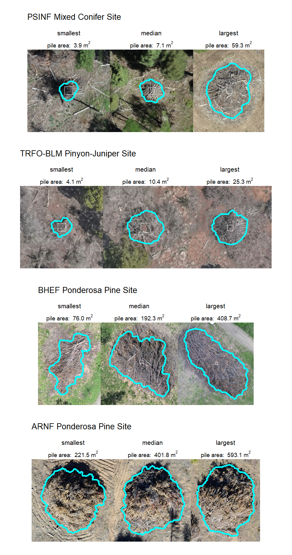
PSINF Mixed Conifer Site	121	9.8	9.4	3.9-59.3	3.8	1.3	2.6-10.2	3.4	1.2	2.4-9.0	2.2	0.8	1.5-6.4
TRFO-BLM Pinyon-Juniper Site	276	10.6	3.2	4.1-25.3	4.2	0.6	2.6-6.4	NA	NA	NA	NA	NA	NA
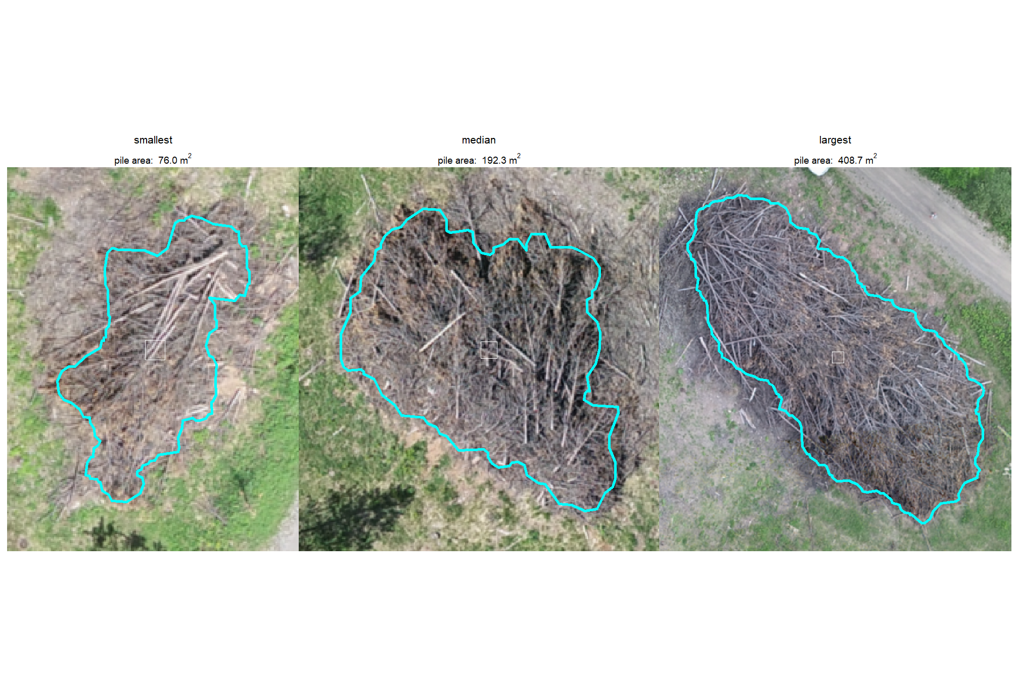
BHEF Ponderosa Pine Site	26	199.9	85.8	76.0-408.7	21.0	6.5	13.3-38.0	NA	NA	NA	NA	NA	NA
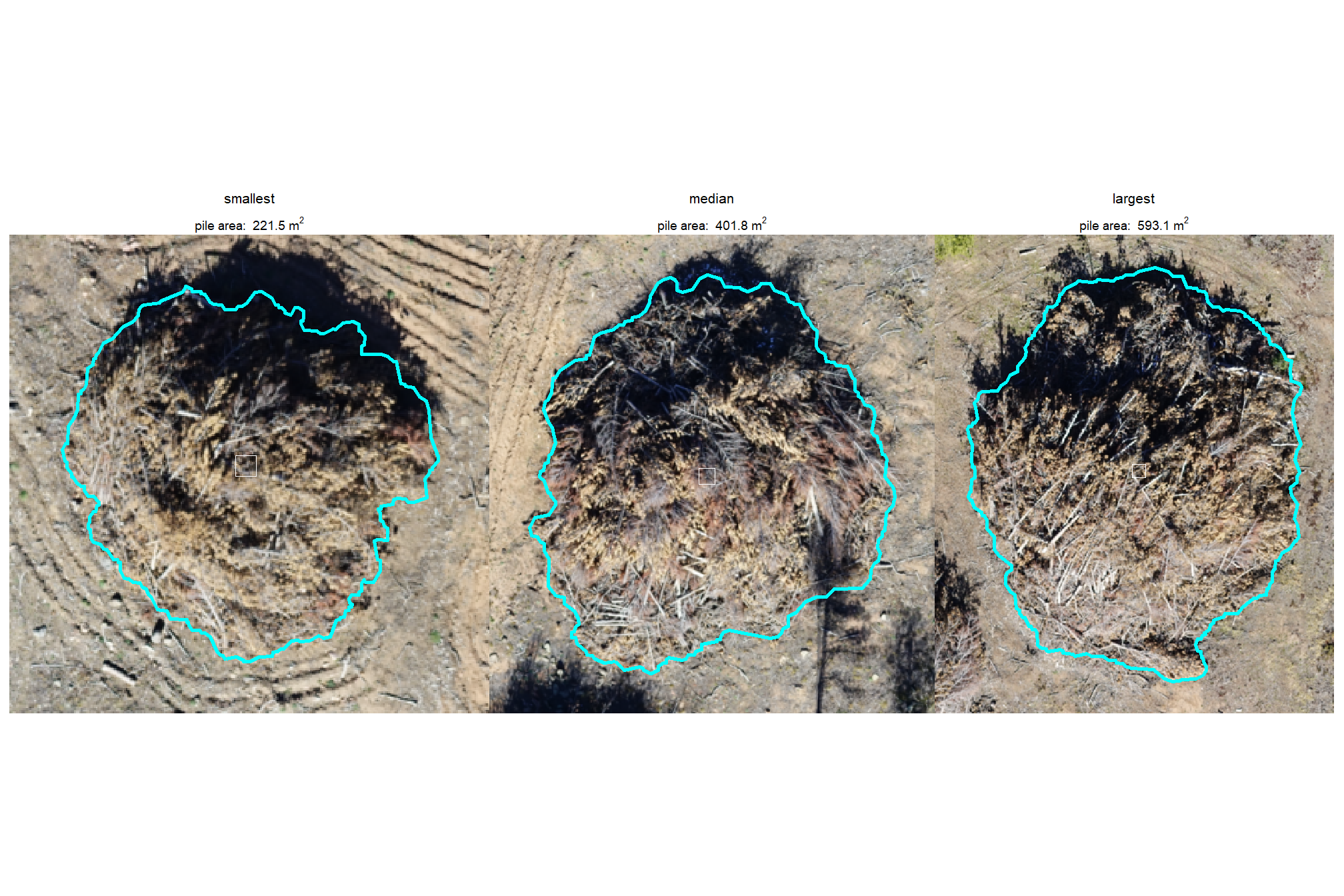
ARNF Ponderosa Pine Site	19	409.0	97.1	221.5-593.1	25.9	3.6	18.4-32.9	NA	NA	NA	NA	NA	NA

All sites except PSINF have only mechanical or only hand piles whereas PSINF has both hand piles and mechanical piles. Let’s look at the summary statistics for the form measurements for only PSINF based on pile construction type

psinf_slash_piles_polys %>% 
  sf::st_drop_geometry() %>% 
  dplyr::filter(is_in_stand) %>% 
  dplyr::select(
    -tidyselect::contains("volume_m3")
    , -tidyselect::starts_with("field_gt_area")
    , -c(site)
  ) %>% 
  dplyr::rename(pile_type = comment) %>% 
  dplyr::group_by(pile_type) %>% 
  agg_piles_temp() %>% 
  dplyr::select(
    pile_type, n
    , tidyselect::starts_with("image_")
    , tidyselect::starts_with("field_")
  ) %>% 
  kbl_form_sum_stats_wide(by_lab = "PSINF Mixed Conifer Site by pile type")  

Table 2.3: Slash pile image-annotated and field-collected form measurements
PSINF Mixed Conifer Site by pile type

		Image-Ann. Area (m2)			Image-Ann. Diam (m)			Field-Meas. Diam (m)			Field-Meas. Height (m)
	Piles	Mean	Std Dev	Range	Mean	Std Dev	Range	Mean	Std Dev	Range	Mean	Std Dev	Range
Hand Pile	111	7.2	1.7	3.9-14.3	3.5	0.4	2.6-5.0	3.1	0.3	2.4-4.3	2.0	0.2	1.5-2.4
Mechanical Pile	10	38.3	12.7	21.3-59.3	8.0	1.3	5.9-10.2	7.2	1.1	5.5-9.0	4.4	1.2	2.4-6.4

2.2.3 Image-Annotation Comparison

For only the PSINF site, let’s check the field-collected and image-annotated measurements of diameter which will serve as a good sanity check for our image-annotation process (assuming diameter was accurately measured in the field…might be a perilous assumption)

psinf_slash_piles_polys %>% 
  dplyr::mutate(diff_diameter_m = image_gt_diameter_m - field_diameter_m) %>% 
  ggplot2::ggplot(mapping = ggplot2::aes(x = image_gt_diameter_m, y = field_diameter_m)) +
  ggplot2::geom_abline(lwd = 1.5) +
  ggplot2::geom_point(ggplot2::aes(color = diff_diameter_m)) +
  ggplot2::geom_smooth(method = "lm", se=F, color = "tomato", linetype = "dashed") +
  ggplot2::scale_color_viridis_c(option = "mako", direction = -1, alpha = 0.8) +
  ggplot2::scale_x_continuous(limits = c(0, max( max(psinf_slash_piles_polys$field_diameter_m,na.rm=T), max(psinf_slash_piles_polys$image_gt_diameter_m,na.rm=T) ) )) +
  ggplot2::scale_y_continuous(limits = c(0, max( max(psinf_slash_piles_polys$field_diameter_m,na.rm=T), max(psinf_slash_piles_polys$image_gt_diameter_m,na.rm=T) ) )) +
  ggplot2::labs(
    x = "image-annotated diameter (m)", y = "field-collected diameter (m)"
    , color = "image-field\ndiameter diff."
    , subtitle = "diameter (m) comparison"
  ) +
  ggplot2::theme_light()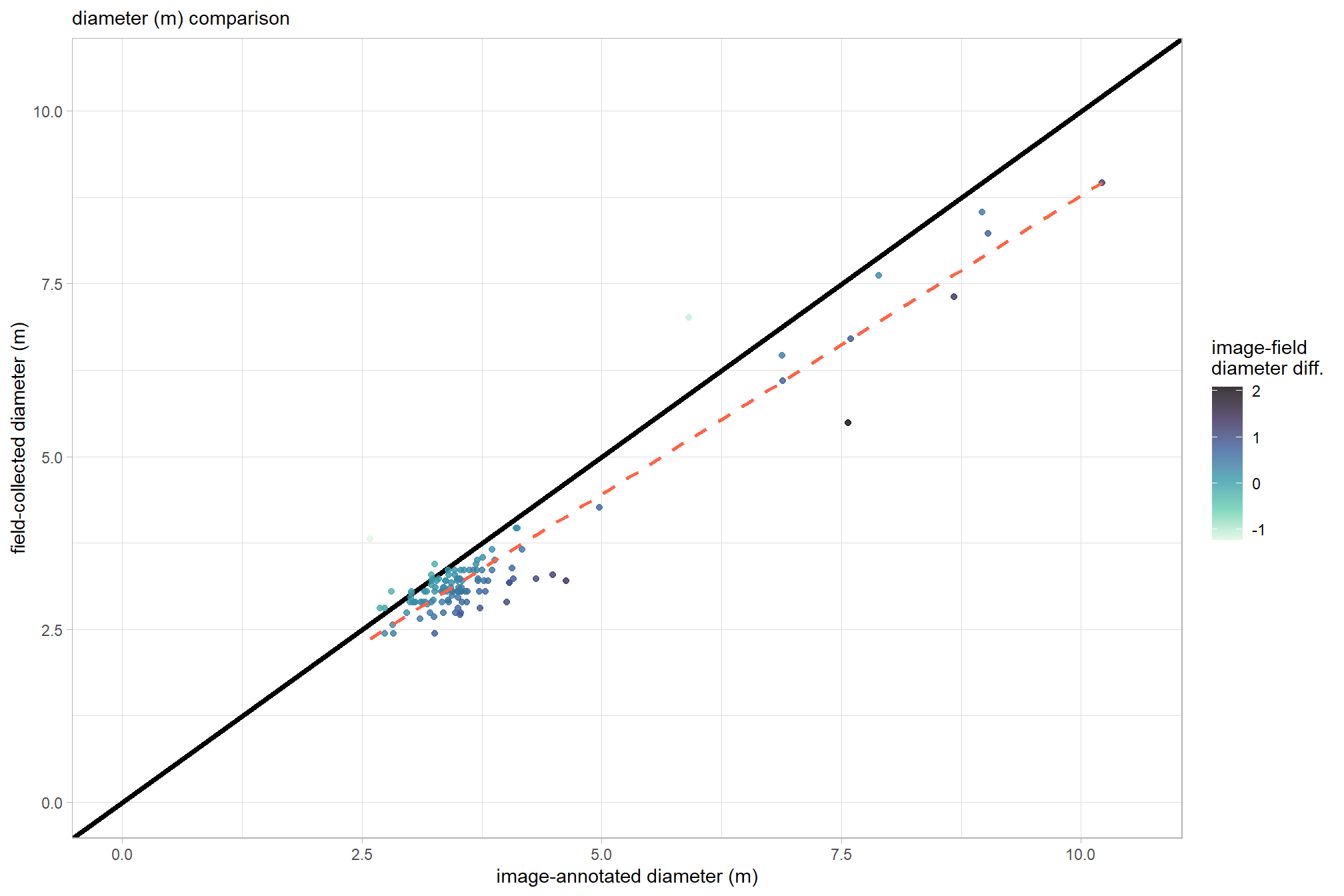

the plot makes these values look very similar with the image-annotated diameter generally larger than the field-collected value. let’s check these using lm()

lm_temp <- lm(field_diameter_m ~ image_gt_diameter_m, data = psinf_slash_piles_polys)
summary(lm_temp)

## 
## Call:
## lm(formula = field_diameter_m ~ image_gt_diameter_m, data = psinf_slash_piles_polys)
## 
## Residuals:
##      Min       1Q   Median       3Q      Max 
## -1.18985 -0.16525  0.01416  0.16807  1.76883 
## 
## Coefficients:
##                     Estimate Std. Error t value Pr(>|t|)    
## (Intercept)          0.13522    0.09891   1.367    0.174    
## image_gt_diameter_m  0.86403    0.02436  35.471   <2e-16 ***
## ---
## Signif. codes:  0 '***' 0.001 '**' 0.01 '*' 0.05 '.' 0.1 ' ' 1
## 
## Residual standard error: 0.3593 on 119 degrees of freedom
##   (66 observations deleted due to missingness)
## Multiple R-squared:  0.9136, Adjusted R-squared:  0.9129 
## F-statistic:  1258 on 1 and 119 DF,  p-value: < 2.2e-16

Our slope of 0.86 is close to 1 and, along with our high R-squared value of 91%, indicate our image- and field-measured diameters are well-calibrated

let’s use a paired t-test to determine if the mean difference (MD) between the field-measured diameter and the image-annotated diameter is statistically significant (i.e. significantly different from zero)

# is the mean difference between the two diameters significantly different from zero
ttest_temp <- t.test(
  psinf_slash_piles_polys %>% 
    dplyr::filter(!is.na(field_diameter_m), !is.na(image_gt_diameter_m)) %>% 
    dplyr::pull(field_diameter_m)
  , psinf_slash_piles_polys %>% 
    dplyr::filter(!is.na(field_diameter_m), !is.na(image_gt_diameter_m)) %>% 
    dplyr::pull(image_gt_diameter_m)
  , paired = TRUE
)
ttest_temp

## 
##  Paired t-test
## 
## data:  psinf_slash_piles_polys %>% dplyr::filter(!is.na(field_diameter_m), !is.na(image_gt_diameter_m)) %>% dplyr::pull(field_diameter_m) and psinf_slash_piles_polys %>% dplyr::filter(!is.na(field_diameter_m), !is.na(image_gt_diameter_m)) %>% dplyr::pull(image_gt_diameter_m)
## t = -10.563, df = 120, p-value < 2.2e-16
## alternative hypothesis: true mean difference is not equal to 0
## 95 percent confidence interval:
##  -0.4583169 -0.3136208
## sample estimates:
## mean difference 
##      -0.3859688

the mean difference (MD) is -0.39 m (field-measured minus image-annotated value). also, the p-value of 0.00001 is less than 0.05, meaning we should reject the null hypothesis that the true mean difference is zero. this confirms that the systematic difference (or bias) we observed where image-annotated diameter is larger than the field-measured diameter is statistically significant and not due to random chance

2.3 RGB orthomosaic

Orthomosaic tif files from UAS flight imagery were created in the photogrammetry software (e.g. Agisoft Metashape). Each of our study sites have RGB data available covering the study area extent.

We’re going to standardize the raster resolution of these RGB data across study sites. The RGB orthomosaics created from UAS photogrammetry processing generally have very fine resolutions of 4 cm or finer and we will standardize the data to make it slightly more coarse (6 cm) to reduce the computational processing burden.

my_rgb_res_m <- 0.06

2.3.1 PSINF Mixed Conifer Site

load the original data

#### read RGB data keep only RGB
psinf_rgb_rast <- terra::rast(
    file.path(
      # "f:/PFDP_Data\\p4pro_images\\P4Pro_06_17_2021_half_half_optimal\\3_dsm_ortho\\2_mosaic"
      # , "P4Pro_06_17_2021_half_half_optimal_transparent_mosaic_group1.tif"
      "../data/Dawson_Data/dawson_rgb.tif"
    )
  ) %>% 
  terra::subset(c(1,2,3))
# rename bands
names(psinf_rgb_rast) <- c("red","green","blue")

what is the resolution of the original RGB data?

terra::res(psinf_rgb_rast)

## [1] 0.025883 0.025883

let’s reduce the resolution (i.e. increase the raster cell size; make more coarse)

## function to change the resolution of RGB 
change_res_fn <- function(
  r
  , my_res=1
  , m = "bilinear"
  # , ofile = tempfile(fileext = ".tif")
  , ofile = NULL
){
  if(terra::res(r)[1] == my_res){
    return(r)
  }else{
    r2 <- r
    terra::res(r2) <- my_res
    if(!inherits(ofile,"character")){
      r2 <- terra::resample(r, r2, method = m) 
    }else{
      r2 <- terra::resample(r, r2, method = m, filename=ofile, overwrite = T) 
    }
    return(r2) 
  }
}
###############################################################
# clip to boundary and resample to change resolution
###############################################################
dir_temp <- "../data/PFDP_Data/"
rgb_fnm_temp <- file.path(dir_temp,"psinf_rgb_rast.tif") # what should the compiled rgb be called?
if(!dir.exists(dir_temp)){dir.create(dir_temp, showWarnings = F)}
if(!file.exists(rgb_fnm_temp)){
  # Crop the raster to the rectangular extent of the polygon
  # Specify a filename to ensure the result is written to disk
  crop_rgb_rast_temp <- psinf_rgb_rast %>% 
    terra::crop(
      psinf_stand_boundary %>% 
        sf::st_union() %>% 
        sf::st_buffer(10) %>% 
        terra::vect() %>% 
        terra::project(terra::crs(psinf_rgb_rast))
      , filename =  tempfile(fileext = ".tif")
      , overwrite = TRUE
    ) 
  # Mask the cropped raster to the precise shape of the polygon
  # This function will also be processed on disk due to the file size
  psinf_rgb_rast <- terra::mask(
    crop_rgb_rast_temp
    , psinf_stand_boundary %>% 
      sf::st_union() %>% 
      sf::st_buffer(10) %>% 
      terra::vect() %>% 
      terra::project(terra::crs(psinf_rgb_rast))
    , filename = tempfile(fileext = ".tif")
    , overwrite = TRUE
  )
  
  ## apply the change_res_fn for our analysis we don't need such finery
  # this takes too long...
  psinf_rgb_rast <- change_res_fn(psinf_rgb_rast, my_res=my_rgb_res_m, ofile = rgb_fnm_temp)
}else{
  psinf_rgb_rast <- terra::rast(rgb_fnm_temp)
}
# terra::res(psinf_rgb_rast)
# terra::plotRGB(bhef_rgb_rast, stretch = "lin")

make a function to plot the RGB imagery as a background for ggplot2 plots. ggplot2 offers capabilities to build multi-layered, publication-quality figures by stacking multiple vector overlays on an RGB background. however, it can be computationally expensive since it requires the conversion to a data frame first.

# make a function to plot these detected crowns with rgb data
ortho_plt_fn <- function(rgb_rast, stand, add_stand = F, buffer = 10, plt_lwd = 1, plt_line_col = "black"){
  if(!inherits(rgb_rast,"SpatRaster")){stop("rgb_rast must be terra SpatRaster data")}
  if(terra::nlyr(rgb_rast)<3){stop("rgb_rast must have 3 layers with RGB data")}
  if(!inherits(stand,"sf") && !inherits(stand,"sfc")){stop("stand must be sf data")}
  # crop
  crp_rgb_rast_temp <- rgb_rast %>% 
    terra::crop(
      stand %>% 
        dplyr::ungroup() %>% 
        sf::st_union() %>% 
        sf::st_bbox() %>% 
        sf::st_as_sfc() %>% 
        sf::st_buffer(buffer) %>% 
        sf::st_transform(terra::crs(rgb_rast)) %>% 
        terra::vect()
    )
  # convert raster to a data frame and create hex colors
  # ?grDevices::rgb
  rgb_df_temp <-
    crp_rgb_rast_temp %>% 
    terra::as.data.frame(xy = TRUE) %>%
    dplyr::rename(
      red = 3, green = 4, blue = 5
    ) %>%
    dplyr::mutate(
      # rows that have missing color data
      is_missing = is.na(red) | is.na(green) | is.na(blue)
      # hex using 0s for NAs to avoid grDevices::rgb error
      , hex_col = grDevices::rgb(
        ifelse(is_missing, 0, red)
        , ifelse(is_missing, 0, green)
        , ifelse(is_missing, 0, blue)
        , maxColorValue = 255
      )
      # back to NA
      , hex_col = ifelse(is_missing, as.character(NA), hex_col)
    ) %>%
    dplyr::select(-c(is_missing))
  
  # plt
  plt <- ggplot2::ggplot() +
    # add rgb base map
    ggplot2::geom_tile(data = rgb_df_temp, mapping = ggplot2::aes(x = x, y = y, fill = hex_col), color = NA) +
    # use identity scale so the hex codes are used directly
    ggplot2::scale_fill_identity(na.value = "transparent") + # !!! don't take this out or RGB plot will kill your computer
    ggplot2::scale_x_continuous(expand = c(0, 0)) +
    ggplot2::scale_y_continuous(expand = c(0, 0)) +
    ggplot2::coord_sf(expand = F) +
    ggplot2::theme_void() +
    ggplot2::theme(
      legend.position = "none"
    )
  # add stand
  if(add_stand){
    # overlay polygons
    plt <- plt +
      # ggplot2::geom_sf(data = polys, fill = NA, color = "red", linewidth = 0.5) +
      ggplot2::geom_sf(
        data = stand %>% 
          sf::st_make_valid() %>% 
          dplyr::filter(sf::st_is_valid(.)) %>% 
          sf::st_transform(terra::crs(rgb_rast))
        , fill = NA
        , color = plt_line_col
        , lwd = plt_lwd
        , inherit.aes = F
      )
  }
  return(plt)
}

test our plotting function on a zoomed-in portion of the study area

ortho_plt_fn(
  psinf_rgb_rast
  , psinf_stand_boundary %>% 
    sf::st_centroid() %>% 
    sf::st_buffer(11)
)

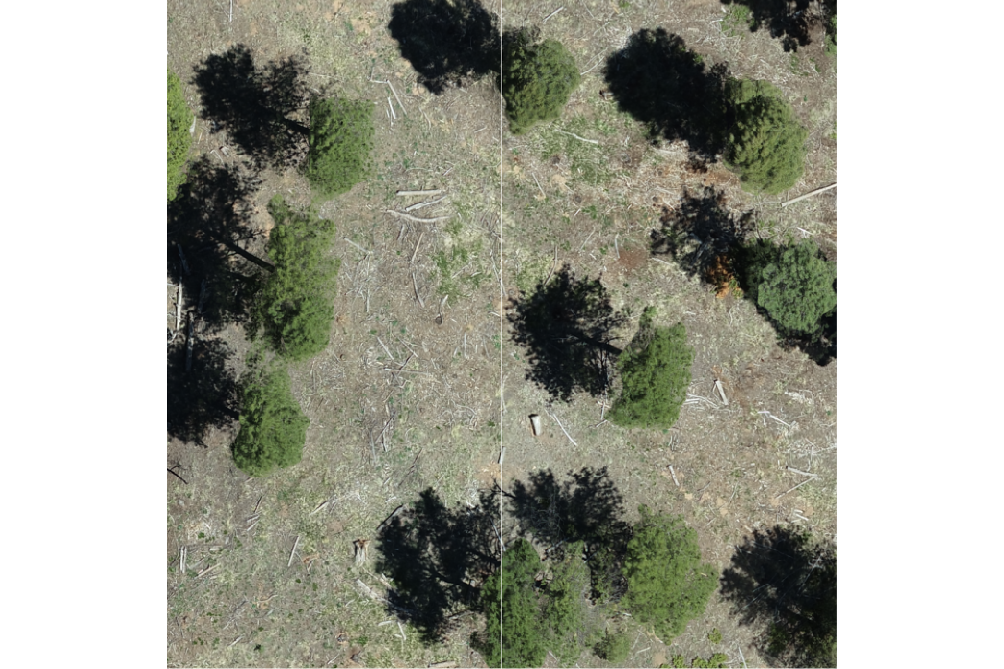
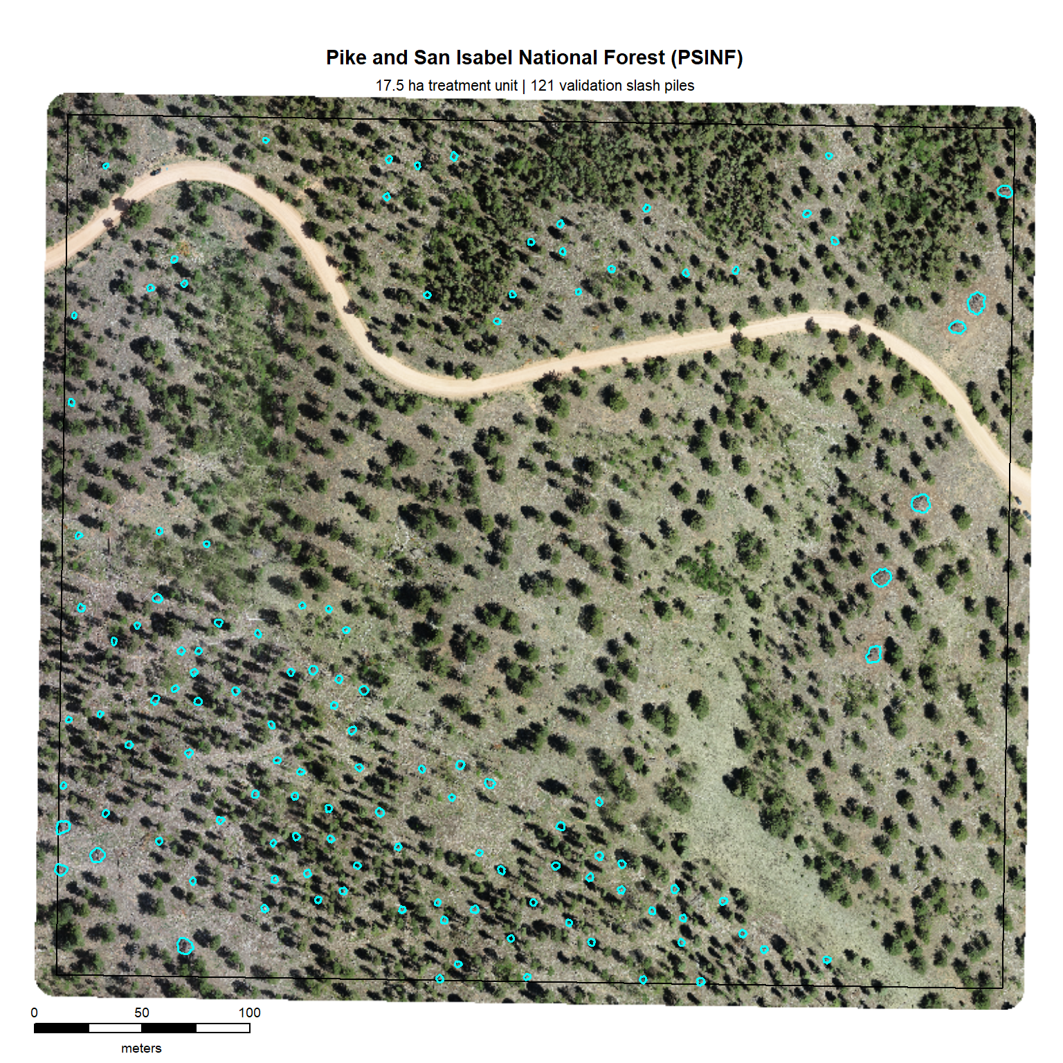
for the entire study area, plotting with terra is much more computationally efficient. let’s plot the RGB data with the stand boundary (black) and image annotated pile footprints (cyan)

# grDevices::jpeg("../data/psinf_stand_rgb.jpeg", width = 8, height = 8, units = "in", res = 300)
# mar = c(bottom, left, top, right)
terra::plotRGB(psinf_rgb_rast, mar=c(2, 0.5, 3.5, 0.2)) # , stretch="lin"
# add stand boundary
terra::plot(
  psinf_stand_boundary %>% 
    terra::vect() %>% 
    terra::project(terra::crs(psinf_rgb_rast))
  , add = T, border = "black", col = NA, lwd = 1.2
)
# add pile boundaries
terra::plot(
  psinf_slash_piles_polys %>% 
    dplyr::filter(is_in_stand) %>% 
    terra::vect() %>% 
    terra::project(terra::crs(psinf_rgb_rast))
  , add = T, border = "cyan", col = NA, lwd = 1.6
)
# main title top: "side = 3", line = 1
mtext(
  all_stand_boundary %>% 
    sf::st_drop_geometry() %>% 
    dplyr::filter(site_data_lab == "psinf") %>%
    dplyr::pull(site_full_lab)
  # "Pike and San Isabel National Forest (PSINF)"
  , side = 3, line = 1.5, cex = 0.9, font = 2
)
# sub title top: "side = 3", line = 1
mtext(
  paste0(
    all_stand_boundary %>% 
    sf::st_drop_geometry() %>% 
    dplyr::filter(site_data_lab == "psinf") %>% 
    dplyr::mutate(
      site_area_ha = scales::comma(site_area_ha, suffix = " ha treatment unit", accuracy = 0.1)
    ) %>% 
    dplyr::pull(site_area_ha)
    , " | "
    , psinf_slash_piles_polys %>% dplyr::filter(is_in_stand) %>% nrow() %>% scales::comma(accuracy = 1, suffix = " validation slash piles")
  )
  , side = 3, line = 0.5, cex = 0.7
)
# 5. Add scale and north arrow
e_temp <- terra::ext(psinf_rgb_rast)
# 3. Define a position BELOW the minimum Y-coordinate (ymin)
# Subtracting a small value moves it into the bottom margin
scale_x_temp <- e_temp$xmin
scale_y_temp <- e_temp$ymin - ( (e_temp$ymax - e_temp$ymin) * 0.025 ) # 8% below the image
# ?terra::sbar
# have to define the scale bar distance
clean_d_temp <- ceiling((terra::ncol(psinf_rgb_rast)*terra::res(psinf_rgb_rast)[1]*0.2)/10)*10
terra::sbar(
  d = clean_d_temp
  # , xy = "bottomleft"
  , xy = c(scale_x_temp, scale_y_temp)
  , type = "bar"
  , divs = 5
  , below = "meters"
  , labels = c(0, round(clean_d_temp/2), clean_d_temp)
  , adj = c(0.5, -1.5) # adjust label pos c(horz,vert)
  , cex = 0.6
  , xpd = T
)

# # terra::north(xy = "topright", type = 1, cex = 0.6)
# grDevices::dev.off()

2.3.2 TRFO-BLM Pinyon-Juniper Site

load the original data

#### read RGB data keep only RGB
pj_rgb_rast <- terra::rast(
    # "d:/BLM_CO_SWDF_DawsonFuelsTreatment/Final/Ortho/BLM_CO_SWDF_DawsonFuelsTreatment_Ortho_202504.tif"
    "../data/dawson_data/dawson_rgb.tif"
  ) %>% 
  terra::subset(c(1,2,3))
# rename bands
names(pj_rgb_rast) <- c("red","green","blue")

what is the resolution of the original RGB data?

terra::res(pj_rgb_rast)

## [1] 0.025883 0.025883

let’s reduce the resolution (i.e. increase the raster cell size; make more coarse)

###############################################################
# clip to boundary and resample to change resolution
###############################################################
dir_temp <- "../data/dawson_data/"
rgb_fnm_temp <- file.path(dir_temp,"pj_rgb_rast.tif") # what should the compiled rgb be called?
if(!dir.exists(dir_temp)){dir.create(dir_temp, showWarnings = F)}
if(!file.exists(rgb_fnm_temp)){
  # Crop the raster to the rectangular extent of the polygon
  # Specify a filename to ensure the result is written to disk
  crop_rgb_rast_temp <- pj_rgb_rast %>% 
    terra::crop(
      pj_stand_boundary %>% 
        sf::st_union() %>% 
        sf::st_buffer(10) %>% 
        terra::vect() %>% 
        terra::project(terra::crs(pj_rgb_rast))
      , filename =  tempfile(fileext = ".tif")
      , overwrite = TRUE
    ) 
  # Mask the cropped raster to the precise shape of the polygon
  # This function will also be processed on disk due to the file size
  pj_rgb_rast <- terra::mask(
    crop_rgb_rast_temp
    , pj_stand_boundary %>% 
      sf::st_union() %>% 
      sf::st_buffer(10) %>% 
      terra::vect() %>% 
      terra::project(terra::crs(pj_rgb_rast))
    , filename = tempfile(fileext = ".tif")
    , overwrite = TRUE
  )
  
  ## apply the change_res_fn for our analysis we don't need such finery
  # this takes too long...
  pj_rgb_rast <- change_res_fn(pj_rgb_rast, my_res=my_rgb_res_m, ofile = rgb_fnm_temp)
}else{
  pj_rgb_rast <- terra::rast(rgb_fnm_temp)
}

test our ggplot2 plotting function on a zoomed-in portion of the study area

ortho_plt_fn(
  pj_rgb_rast
  , pj_stand_boundary %>% 
    sf::st_centroid() %>% 
    sf::st_buffer(11)
)

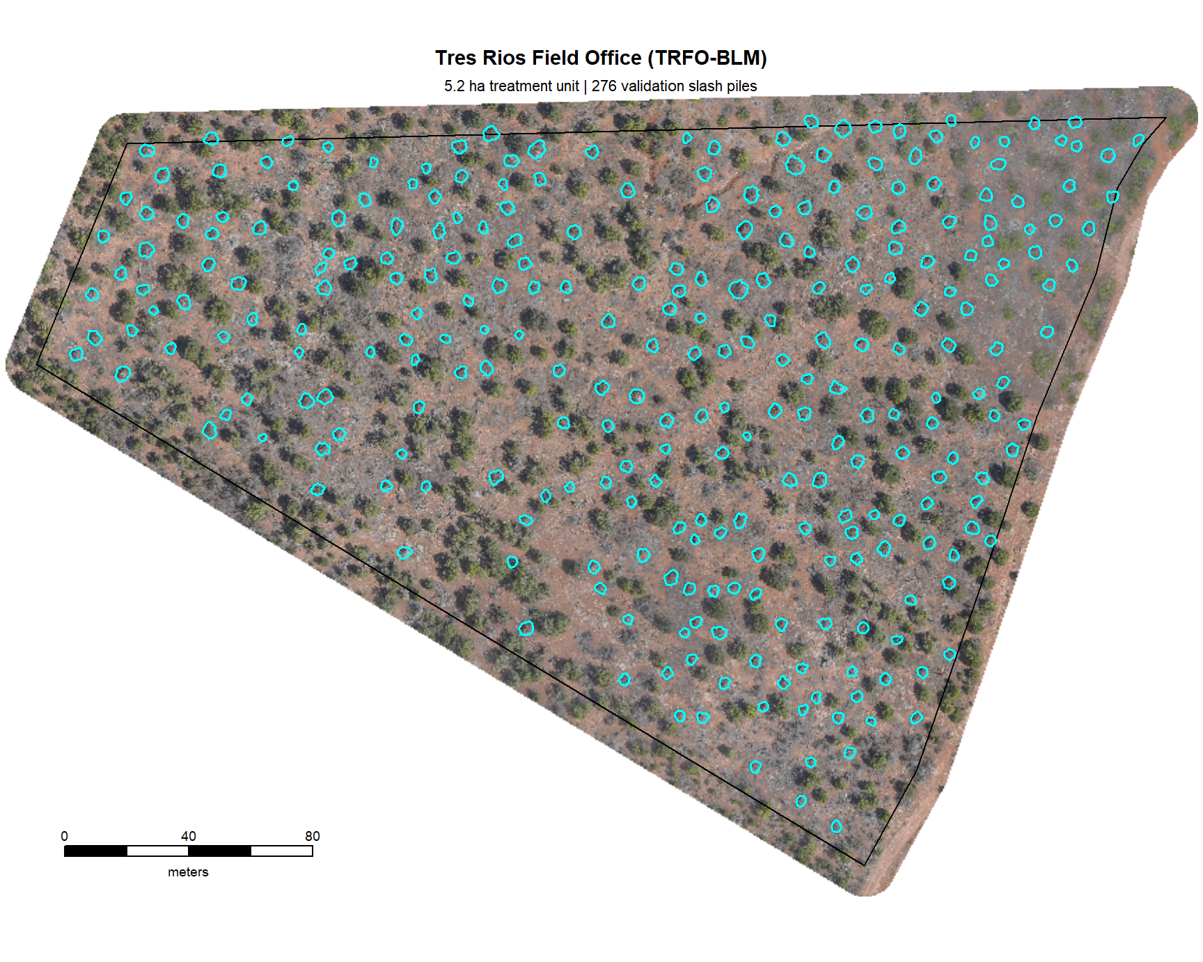
for the entire study area, plotting with terra is much more computationally efficient. let’s plot the RGB data with the stand boundary (black) and image annotated pile footprints (cyan)

# grDevices::jpeg("../data/pj_stand_rgb.jpeg", width = 9, height = 7.2, units = "in", res = 300)
terra::plotRGB(pj_rgb_rast, mar=c(0.2, 0.2, 1, 0.2)) # , stretch="lin"
# add stand boundary
terra::plot(
  pj_stand_boundary %>% 
    terra::vect() %>% 
    terra::project(terra::crs(pj_rgb_rast))
  , add = T, border = "black", col = NA, lwd = 1.2
)
# add pile boundaries
terra::plot(
  pj_slash_piles_polys %>% 
    dplyr::filter(is_in_stand) %>% 
    terra::vect() %>% 
    terra::project(terra::crs(pj_rgb_rast))
  , add = T, border = "cyan", col = NA, lwd = 1.5
)
# main title top: "side = 3", line = 1
mtext(
  all_stand_boundary %>% 
    sf::st_drop_geometry() %>% 
    dplyr::filter(site_data_lab == "pj") %>%
    dplyr::pull(site_full_lab)
  # "Tres Rios Field Office (TRFO-BLM)"
  , side = 3, line = 1.5, cex = 0.9, font = 2
)
# sub title top: "side = 3", line = 1
mtext(
  paste0(
    all_stand_boundary %>% 
    sf::st_drop_geometry() %>% 
    dplyr::filter(site_data_lab == "pj") %>% 
    dplyr::mutate(
      site_area_ha = scales::comma(site_area_ha, suffix = " ha treatment unit", accuracy = 0.1)
    ) %>% 
    dplyr::pull(site_area_ha)
    , " | "
    , pj_slash_piles_polys %>% dplyr::filter(is_in_stand) %>% nrow() %>% scales::comma(accuracy = 1, suffix = " validation slash piles")
  )
  , side = 3, line = 0.5, cex = 0.7
)
# 5. Add scale and north arrow
# ?terra::sbar
# have to define the scale bar distance
clean_d_temp <- ceiling((terra::ncol(pj_rgb_rast)*terra::res(pj_rgb_rast)[1]*0.2)/10)*10
terra::sbar(
  d = clean_d_temp
  , xy = "bottomleft"
  , type = "bar"
  , divs = 5
  , below = "meters"
  , labels = c(0, round(clean_d_temp/2), clean_d_temp)
  , adj = c(0.5, -1.5) # c(horz,vert)
  , cex = 0.6
)

# # terra::north(xy = "topright", type = 1, cex = 0.6)
# grDevices::dev.off()

2.3.3 BHEF Ponderosa Pine Site

load the original data. for this site, the orthomosaics are split across multiple files. we’ll read in each, align the resolutions, and use terra::moasaic() to combine

###############################################################
# compile RGB raster
###############################################################
rgb_dir_temp <- "F:/UAS_Collections/BHEF_202306" # where is the raw las and rgb data?
dir_temp <- "../data/BHEF_202306/" # where do you want to save processed data to?
rgb_fnm_temp <- file.path(dir_temp,"bhef_rgb.tif") # what should the compiled rgb be called?
if(!dir.exists(dir_temp)){dir.create(dir_temp, showWarnings = F)}
if(!file.exists(rgb_fnm_temp)){
  # read list of orthos
    ortho_list_temp <- list.files(
        rgb_dir_temp
        , pattern = ".*(_RGB|_RBG)\\.(tif|tiff)$"
        , full.names = T, recursive = T
      ) %>% 
      purrr::map(function(x){terra::rast(x)})
    ## apply the change_res_fn
    ortho_list_temp <- 1:length(ortho_list_temp) %>% 
      purrr::map(function(x){change_res_fn(ortho_list_temp[[x]], my_res=0.04)})
    ######## mosaic the raster list 
    bhef_rgb_rast <- terra::mosaic(
      terra::sprc(ortho_list_temp)
      , fun = "min" # min only thing that works
      , filename = rgb_fnm_temp
      , overwrite = T
    )
}else{
  bhef_rgb_rast <- terra::rast(rgb_fnm_temp) %>% 
    terra::subset(c(1,2,3))
}
# rename bands
names(bhef_rgb_rast) <- c("red","green","blue")

what is the resolution of the original RGB data?

terra::res(bhef_rgb_rast)

## [1] 0.04 0.04

let’s reduce the resolution (i.e. increase the raster cell size; make more coarse). for the sites with machine piles only (BHEF and ARNF), we’ll only slightly increase the RGB resolution to 0.08m compared to the sites with hand piles which use a 0.06m resolution

my_rgb_res_m <- 0.08
###############################################################
# clip to boundary and resample to change resolution
###############################################################
dir_temp <- "../data/BHEF_202306/"
rgb_fnm_temp <- file.path(dir_temp,"bhef_rgb_rast.tif") # what should the compiled rgb be called?
if(!dir.exists(dir_temp)){dir.create(dir_temp, showWarnings = F)}
if(!file.exists(rgb_fnm_temp)){
  # Crop the raster to the rectangular extent of the polygon
  # Specify a filename to ensure the result is written to disk
  crop_rgb_rast_temp <- bhef_rgb_rast %>% 
    terra::crop(
      bhef_stand_boundary %>% 
        sf::st_union() %>% 
        sf::st_buffer(10) %>% 
        terra::vect() %>% 
        terra::project(terra::crs(bhef_rgb_rast))
      , mask = T
      , filename = tempfile(fileext = ".tif")
      , overwrite = TRUE
    ) 
  
  ## apply the change_res_fn for our analysis we don't need such finery
  # this takes too long...
  bhef_rgb_rast <- change_res_fn(crop_rgb_rast_temp, my_res=my_rgb_res_m, ofile = rgb_fnm_temp)
}else{
  bhef_rgb_rast <- terra::rast(rgb_fnm_temp)
}

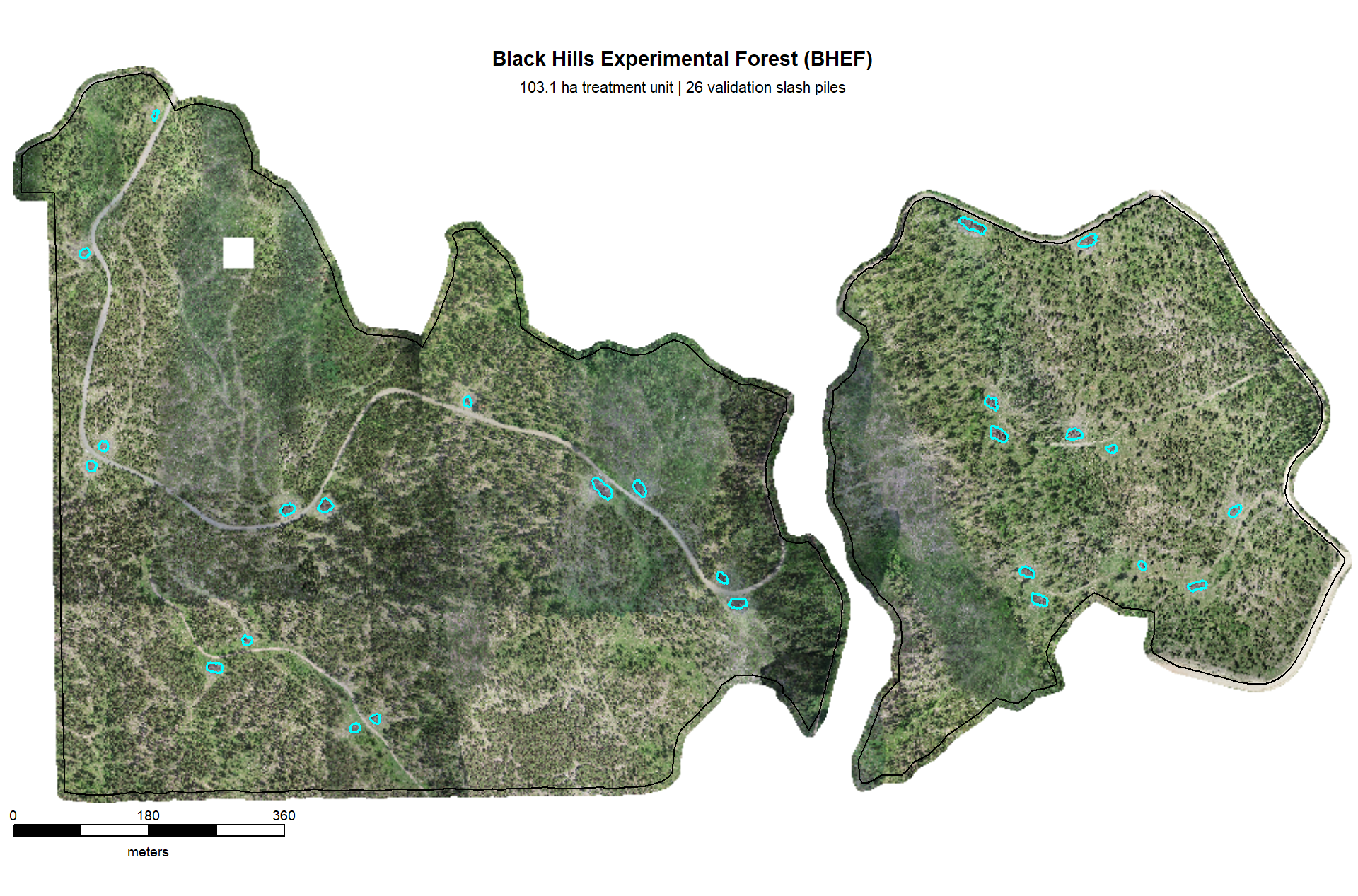
for the entire study area, plotting with terra is much more computationally efficient. let’s plot the RGB data with the stand boundary (black) and image annotated pile footprints (cyan)

# grDevices::jpeg("../data/bhef_stand_rgb.jpeg", width = 10, height = 6.6, units = "in", res = 300)
# mar = c(bottom, left, top, right)
terra::plotRGB(bhef_rgb_rast, mar=c(1.5, 0.5, 0.5, 0.2)) # , stretch="lin"
# add stand boundary
terra::plot(
  bhef_stand_boundary %>% 
    terra::vect() %>% 
    terra::project(terra::crs(bhef_rgb_rast))
  , add = T, border = "black", col = NA, lwd = 1.2
)
# add pile boundaries
terra::plot(
  bhef_slash_piles_polys %>% 
    dplyr::filter(is_in_stand) %>% 
    terra::vect() %>% 
    terra::project(terra::crs(bhef_rgb_rast))
  , add = T, border = "cyan", col = NA, lwd = 1.6
)
# main title top: "side = 3", line = 1
mtext(
  all_stand_boundary %>% 
    sf::st_drop_geometry() %>% 
    dplyr::filter(site_data_lab == "bhef") %>%
    dplyr::pull(site_full_lab)
  , side = 3, line = 1.5, cex = 0.9, font = 2
)
# sub title top: "side = 3", line = 1
mtext(
  paste0(
    all_stand_boundary %>% 
    sf::st_drop_geometry() %>% 
    dplyr::filter(site_data_lab == "bhef") %>% 
    dplyr::mutate(
      site_area_ha = scales::comma(site_area_ha, suffix = " ha treatment unit", accuracy = 0.1)
    ) %>% 
    dplyr::pull(site_area_ha)
    , " | "
    , bhef_slash_piles_polys %>% dplyr::filter(is_in_stand) %>% nrow() %>% scales::comma(accuracy = 1, suffix = " validation slash piles")
  )
  , side = 3, line = 0.5, cex = 0.7
)
# 5. Add scale and north arrow
e_temp <- terra::ext(bhef_rgb_rast)
# 3. Define a position BELOW the minimum Y-coordinate (ymin)
# Subtracting a small value moves it into the bottom margin
scale_x_temp <- e_temp$xmin
scale_y_temp <- e_temp$ymin - ( (e_temp$ymax - e_temp$ymin) * 0.045 ) # 8% below the image
# ?terra::sbar
# have to define the scale bar distance
clean_d_temp <- ceiling((terra::ncol(bhef_rgb_rast)*terra::res(bhef_rgb_rast)[1]*0.2)/10)*10
terra::sbar(
  d = clean_d_temp
  # , xy = "bottomleft"
  , xy = c(scale_x_temp, scale_y_temp)
  , type = "bar"
  , divs = 5
  , below = "meters"
  , labels = c(0, round(clean_d_temp/2), clean_d_temp)
  , adj = c(0.5, -1.5) # adjust label pos c(horz,vert)
  , cex = 0.6
  , xpd = T
)

# terra::north(xy = "topright", type = 1, cex = 0.6)
# grDevices::dev.off()

2.3.4 ARNF Ponderosa Pine Site

load the original data

#### read RGB data keep only RGB
arnf_rgb_rast <- terra::rast(
    # "f:/UAS_Collections/ARNF_DiamondView_202510/DiamondPeak_Switchblade_transparent_mosaic_group1.tif"
    "../data/ARNF_DiamondView_202510/arnf_rgb_rast.tif"
  ) %>% 
  terra::subset(c(1,2,3))
# rename bands
names(arnf_rgb_rast) <- c("red","green","blue")

what is the resolution of the original RGB data?

terra::res(arnf_rgb_rast)

## [1] 0.08 0.08

let’s reduce the resolution (i.e. increase the raster cell size; make more coarse)

###############################################################
# clip to boundary and resample to change resolution
###############################################################
dir_temp <- "../data/ARNF_DiamondView_202510/"
rgb_fnm_temp <- file.path(dir_temp,"arnf_rgb_rast.tif") # what should the compiled rgb be called?
if(!dir.exists(dir_temp)){dir.create(dir_temp, showWarnings = F)}
if(!file.exists(rgb_fnm_temp)){
  # Crop the raster to the rectangular extent of the polygon
  # Specify a filename to ensure the result is written to disk
  crop_rgb_rast_temp <- arnf_rgb_rast %>% 
    terra::crop(
      arnf_stand_boundary %>% 
        sf::st_union() %>% 
        sf::st_buffer(10) %>% 
        terra::vect() %>% 
        terra::project(terra::crs(arnf_rgb_rast))
      , mask = T
      , filename =  tempfile(fileext = ".tif")
      , overwrite = TRUE
    ) 
  
  ## apply the change_res_fn for our analysis we don't need such finery
  # this takes too long...
  arnf_rgb_rast <- change_res_fn(crop_rgb_rast_temp, my_res=my_rgb_res_m, ofile = rgb_fnm_temp)
}else{
  arnf_rgb_rast <- terra::rast(rgb_fnm_temp)
}

test our ggplot2 plotting function on a zoomed-in portion of the study area

ortho_plt_fn(
  arnf_rgb_rast
  , arnf_stand_boundary %>% 
    sf::st_centroid() %>% 
    sf::st_buffer(11)
)

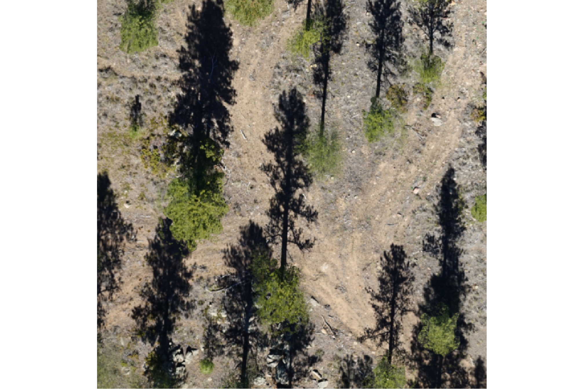
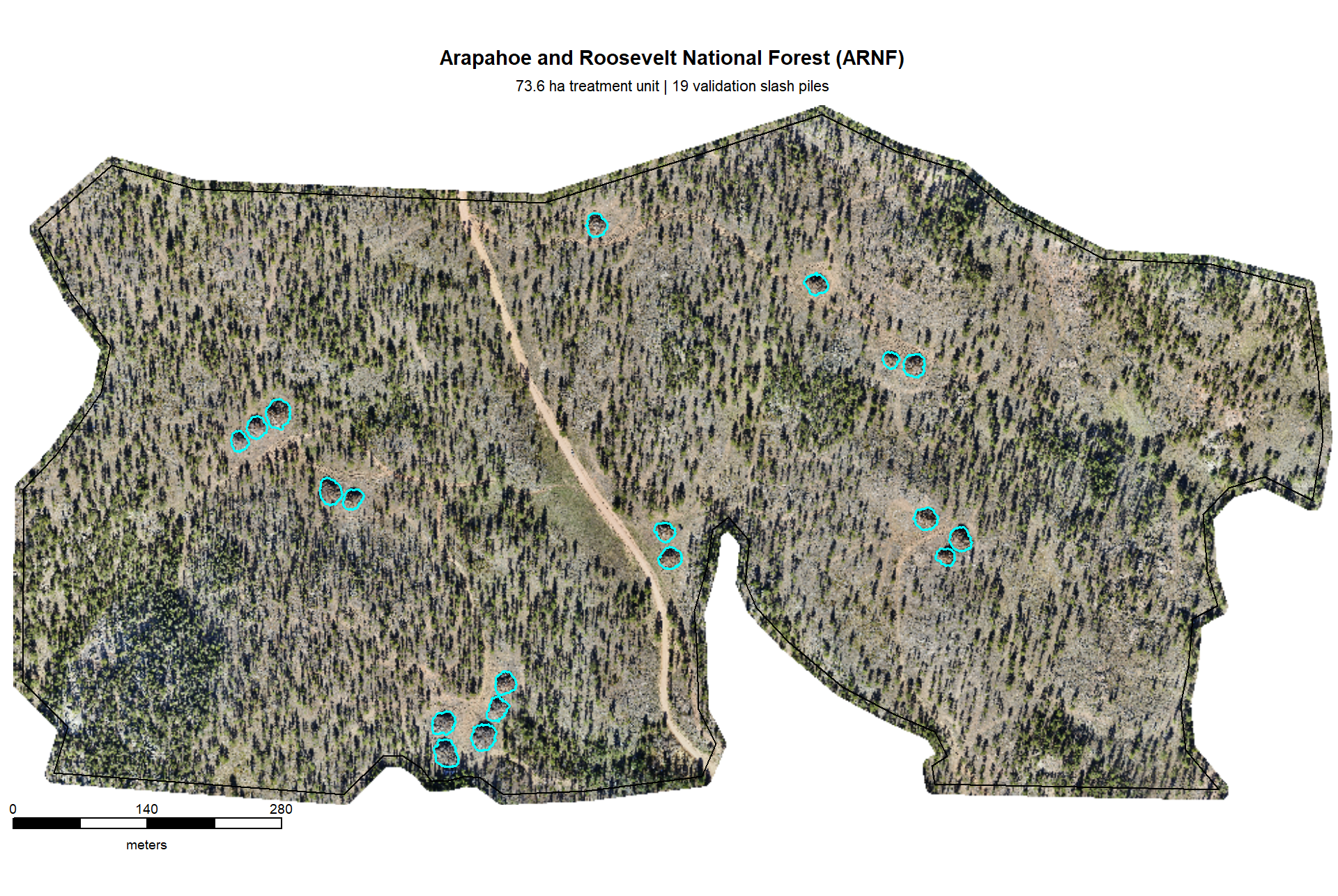
for the entire study area, plotting with terra is much more computationally efficient. let’s plot the RGB data with the stand boundary (black) and image annotated pile footprints (cyan)

# grDevices::jpeg("../data/arnf_stand_rgb.jpeg", width = 10, height = 6.7, units = "in", res = 300)
# mar = c(bottom, left, top, right)
terra::plotRGB(arnf_rgb_rast, mar=c(0.5, 0.5, 1, 0.2)) # , stretch="lin"
# add stand boundary
terra::plot(
  arnf_stand_boundary %>% 
    terra::vect() %>% 
    terra::project(terra::crs(arnf_rgb_rast))
  , add = T, border = "black", col = NA, lwd = 1.2
)
# add pile boundaries
terra::plot(
  arnf_slash_piles_polys %>% 
    dplyr::filter(is_in_stand) %>% 
    terra::vect() %>% 
    terra::project(terra::crs(arnf_rgb_rast))
  , add = T, border = "cyan", col = NA, lwd = 1.6
)
# main title top: "side = 3", line = 1
mtext(
  all_stand_boundary %>% 
    sf::st_drop_geometry() %>% 
    dplyr::filter(site_data_lab == "arnf") %>%
    dplyr::pull(site_full_lab)
  # "Arapahoe and Roosevelt National Forest (ARNF)"
  , side = 3, line = 1.5, cex = 0.9, font = 2
)
# sub title top: "side = 3", line = 1
mtext(
  paste0(
    all_stand_boundary %>% 
    sf::st_drop_geometry() %>% 
    dplyr::filter(site_data_lab == "arnf") %>% 
    dplyr::mutate(
      site_area_ha = scales::comma(site_area_ha, suffix = " ha treatment unit", accuracy = 0.1)
    ) %>% 
    dplyr::pull(site_area_ha)
    , " | "
    , arnf_slash_piles_polys %>% dplyr::filter(is_in_stand) %>% nrow() %>% scales::comma(accuracy = 1, suffix = " validation slash piles")
  )
  , side = 3, line = 0.5, cex = 0.7
)
# 5. Add scale and north arrow
e_temp <- terra::ext(arnf_rgb_rast)
# 3. Define a position BELOW the minimum Y-coordinate (ymin)
# Subtracting a small value moves it into the bottom margin
scale_x_temp <- e_temp$xmin
scale_y_temp <- e_temp$ymin - ( (e_temp$ymax - e_temp$ymin) * 0.035 ) # 8% below the image
# ?terra::sbar
# have to define the scale bar distance
clean_d_temp <- ceiling((terra::ncol(arnf_rgb_rast)*terra::res(arnf_rgb_rast)[1]*0.2)/10)*10
terra::sbar(
  d = clean_d_temp
  # , xy = "bottomleft"
  , xy = c(scale_x_temp, scale_y_temp)
  , type = "bar"
  , divs = 5
  , below = "meters"
  , labels = c(0, round(clean_d_temp/2), clean_d_temp)
  , adj = c(0.5, -1.5) # adjust label pos c(horz,vert)
  , cex = 0.6
  , xpd = T
)

# # terra::north(xy = "topright", type = 1, cex = 0.6)
# grDevices::dev.off()

2.4 Slash Pile RGB Imagery

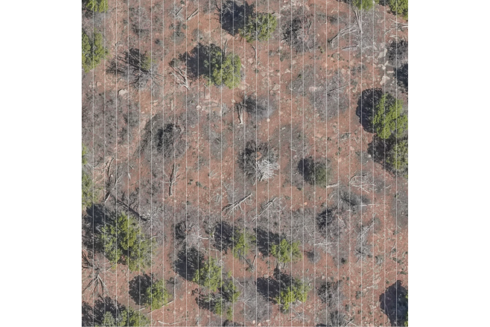
let’s look at the RGB imagery and pile locations. we’ll make a panel of plots for each pile at each study site and place a one square meter box in the middle of each pile to distinguish size

plt_fn_temp <- function(vect, rgb){
  # get vector
  d <- vect %>% 
    dplyr::slice(1) %>% 
    sf::st_transform(terra::crs(rgb))
  # make a box
  sqm <- d %>% 
    sf::st_centroid() %>% 
    sf::st_buffer(
      sqrt(1/4) ## numerator = desired plot size in m2
      , endCapStyle = "SQUARE"
    ) %>%
    dplyr::mutate(dummy=1)
  # buff
  buff <- dplyr::case_when(
    d$image_gt_diameter_m < 4 ~ 4
    , d$image_gt_diameter_m > 10 ~ 2.5
    , T ~ d$image_gt_diameter_m*(2/3)
  )
  # plt
  ortho_plt_fn(
    rgb_rast = rgb
    , stand = sf::st_union(d, sqm)
    , buffer = buff
    , add_stand = F
  ) + 
  ggplot2::geom_sf(data = sqm, fill = NA, color = "white", inherit.aes = F) +
  ggplot2::geom_sf(data = d, fill = NA, lwd = 1, color = "cyan", inherit.aes = F) +
  ggplot2::labs(
    subtitle = base::bquote(
      "pile area: " ~
      .(scales::comma(d$image_gt_area_m2, accuracy = 0.1)) ~ 
      m^2
    )
  ) +
  ggplot2::theme(
    plot.subtitle = ggplot2::element_text(hjust = 0.5, size = 7)
    , plot.title = ggplot2::element_text(hjust = 0.5, size = 8)
  )
}
# plot largest, smallest, and median
samp_plt_fn_temp <- function(piles, ortho) {
  min_temp <-
    plt_fn_temp(
      vect = piles %>% 
        dplyr::filter(is_in_stand) %>% 
        dplyr::ungroup() %>% 
        dplyr::slice_min(n = 1, order_by = image_gt_area_m2, na_rm = T, with_ties = F)
      , rgb = ortho
    ) +
    ggplot2::labs(title = "smallest")
  med_temp <-
    plt_fn_temp(
      vect = piles %>% 
        dplyr::filter(is_in_stand) %>% 
        dplyr::ungroup() %>% 
        dplyr::slice_min(
          n = 1
          , order_by = abs(image_gt_area_m2 - median(image_gt_area_m2, na.rm = TRUE))
          , na_rm = T, with_ties = F
        )
      , rgb = ortho
    ) +
    ggplot2::labs(title = "median")
  max_temp <-
    plt_fn_temp(
      vect = piles %>% 
        dplyr::filter(is_in_stand) %>% 
        dplyr::ungroup() %>% 
        dplyr::slice_max(n = 1, order_by = image_gt_area_m2, na_rm = T, with_ties = F)
      , rgb = ortho
    ) +
    ggplot2::labs(title = "largest")
  # combine
  patchwork::wrap_plots(
    list(min_temp, med_temp, max_temp)
    , ncol = 3
  )
}

2.4.1 PSINF Mixed Conifer Site

example smallest, median, and largest slash pile (red) with a one square meter box for size reference

psinf_samp_plt_fn_temp <- samp_plt_fn_temp(piles = psinf_slash_piles_polys, ortho = psinf_rgb_rast)

psinf_samp_plt_fn_temp

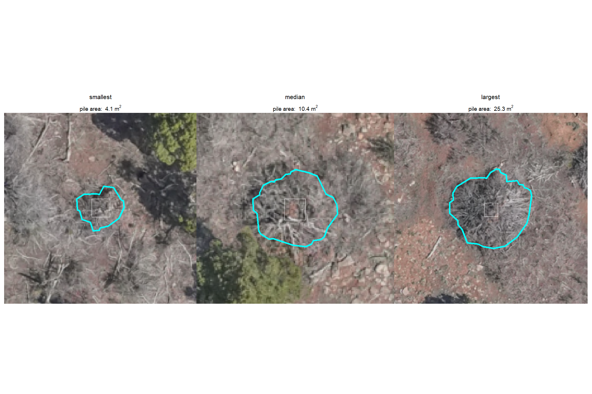
2.4.2 TRFO-BLM Pinyon-Juniper Site

example smallest, median, and largest slash pile (red) with a one square meter box for size reference

pj_samp_plt_fn_temp <- samp_plt_fn_temp(piles = pj_slash_piles_polys, ortho = pj_rgb_rast)

pj_samp_plt_fn_temp

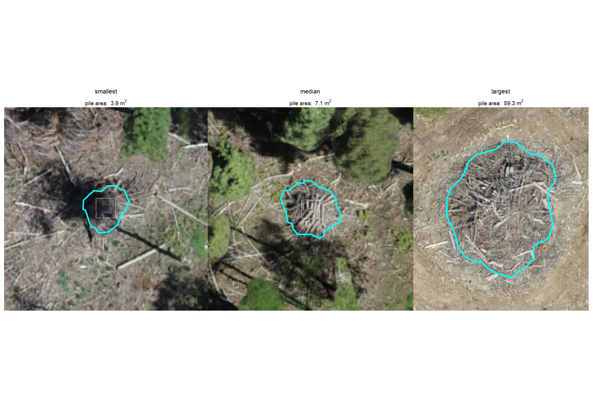
2.4.3 BHEF Ponderosa Pine Site

example smallest, median, and largest slash pile (red) with a one square meter box for size reference

bhef_samp_plt_fn_temp <- samp_plt_fn_temp(piles = bhef_slash_piles_polys, ortho = bhef_rgb_rast)

bhef_samp_plt_fn_temp

2.4.4 ARNF Ponderosa Pine Site

example smallest, median, and largest slash pile (red) with a one square meter box for size reference

arnf_samp_plt_fn_temp <- samp_plt_fn_temp(piles = arnf_slash_piles_polys, ortho = arnf_rgb_rast)

arnf_samp_plt_fn_temp

2.4.5 All

patchwork::wrap_plots(
  patchwork::wrap_elements( 
    psinf_samp_plt_fn_temp + 
      patchwork::plot_annotation(
        title = "PSINF Mixed Conifer Site"
        , theme = ggplot2::theme(plot.title = ggplot2::element_text(size = 10))
      ) 
    )
  , patchwork::wrap_elements( 
    pj_samp_plt_fn_temp + 
      patchwork::plot_annotation(
        title = "TRFO-BLM Pinyon-Juniper Site"
        , theme = ggplot2::theme(plot.title = ggplot2::element_text(size = 10))
      ) 
    )
  , patchwork::wrap_elements( 
    bhef_samp_plt_fn_temp + 
      patchwork::plot_annotation(
        title = "BHEF Ponderosa Pine Site"
        , theme = ggplot2::theme(plot.title = ggplot2::element_text(size = 10))
      ) 
    )
  , patchwork::wrap_elements( 
    arnf_samp_plt_fn_temp + 
      patchwork::plot_annotation(
        title = "ARNF Ponderosa Pine Site"
        , theme = ggplot2::theme(plot.title = ggplot2::element_text(size = 10))
      ) 
    )
  , ncol = 1
)