Section 6 Statistical Analysis: Validation
In this section, we’ll evaluate the influence of the processing parameters on UAS-derived tree detection and monitoring.
The UAS and Field validation data was built and described in this section.
The objective of this study is to determine the influence of different structure from motion (SfM) software (e.g. Agisoft Metashap, OpenDroneMap, Pix4D) and processing parameters on F-score which is a measure of overall tree detection performance.
All of the predictor variables of interest in this study are categorical (a.k.a. factor or nominal) while the predicted variables are metric and include F-score (ranges from 0-1) and error (e.g. MAPE, RMSE). This type of statistical analysis is described in the second edition of Kruschke’s Doing Bayesian data analysis (2015) and here we will build a Bayesian approach based on Kruschke (2015). This analysis was greatly enhanced by A. Solomon Kurz’s ebook supplement to Kruschke (2015).
For a more in-depth review of the traditional treatment of this sort of data structure called multifactor analysis of variance (ANOVA) compared to the Bayesian hierarchical generalization of the traditional ANOVA model used here see this previous section.
6.1 Setup
first we’re going to define a function to ingest a formula as text and separate it into multiple rows based on the number of characters for plotting
# function to pull the formula for labeling below
get_frmla_text = function(frmla_chr, split_chrs = 100){

  cumsum_group = function(x, threshold) {
    cumsum = 0
    group = 1
    result = numeric()
    for (i in 1:length(x)) {
      cumsum = cumsum + x[i]
      if (cumsum > threshold) {
        group = group + 1
        cumsum = x[i]
      }
      result = c(result, group)
    }
    return (result)
  }

  r = stringr::str_sub(
    frmla_chr
    , # get the two column matrix of start end
      frmla_chr %>%
        stringr::str_locate_all("\\+") %>%
        .[[1]] %>%
        dplyr::as_tibble() %>%
        dplyr::select(start) %>%
        dplyr::mutate(
          len = dplyr::coalesce(start-dplyr::lag(start),0)
          , ld = dplyr::coalesce(dplyr::lead(start)-1, stringr::str_length(frmla_chr))
          , cum = cumsum_group(len, split_chrs)
          , start = ifelse(dplyr::row_number()==1,1,start)
        ) %>%
        dplyr::group_by(cum) %>%
        dplyr::summarise(start = min(start), end = max(ld)) %>%
        dplyr::ungroup() %>%
        dplyr::select(-cum) %>%
        as.matrix()
    ) %>%
    stringr::str_squish() %>%
    paste0(collapse = "\n")

  return(r)
}
6.2 Summary Statistics
What is this data?
# load data if needed
if(ls()[ls() %in% "ptcld_validation_data"] %>% length()==0){
 ptcld_validation_data = readr::read_csv("../data/ptcld_full_analysis_data.csv") %>%
   dplyr::mutate(
      depth_maps_generation_quality = factor(
          depth_maps_generation_quality %>%
            tolower() %>%
            stringr::str_replace_all("ultrahigh", "ultra high")
          , ordered = TRUE
          , levels = c(
            "lowest"
            , "low"
            , "medium"
            , "high"
            , "ultra high"
          )
        ) %>% forcats::fct_rev()
      , depth_maps_generation_filtering_mode = factor(
          depth_maps_generation_filtering_mode %>% tolower()
          , ordered = TRUE
          , levels = c(
            "disabled"
            , "mild"
            , "moderate"
            , "aggressive"
          )
        ) %>% forcats::fct_rev()
    )
}
# replace 0 F-score with very small positive to run models
ptcld_validation_data = ptcld_validation_data %>%
  dplyr::mutate(dplyr::across(
    .cols = tidyselect::ends_with("f_score")
    , .fns = ~ ifelse(.x==0,1e-4,.x)
  ))
# what is this data?
ptcld_validation_data %>% dplyr::glimpse()
## Rows: 260
## Columns: 114
## $ tracking_file_full_path <chr> "D:\\SfM_Software_Comparison\\Me…
## $ software <chr> "METASHAPE", "METASHAPE", "METAS…
## $ study_site <chr> "KAIBAB_HIGH", "KAIBAB_HIGH", "K…
## $ processing_attribute1 <chr> "HIGH", "HIGH", "HIGH", "HIGH", …
## $ processing_attribute2 <chr> "AGGRESSIVE", "DISABLED", "MILD"…
## $ processing_attribute3 <chr> NA, NA, NA, NA, NA, NA, NA, NA, …
## $ file_name <chr> "HIGH_AGGRESSIVE", "HIGH_DISABLE…
## $ number_of_points <int> 52974294, 72549206, 69858217, 69…
## $ las_area_m2 <dbl> 86661.27, 87175.42, 86404.78, 86…
## $ timer_tile_time_mins <dbl> 0.63600698, 2.49318542, 0.841338…
## $ timer_class_dtm_norm_chm_time_mins <dbl> 3.6559556, 5.3289152, 5.1638296,…
## $ timer_treels_time_mins <dbl> 8.9065272, 19.2119663, 12.339179…
## $ timer_itd_time_mins <dbl> 0.02202115, 0.02449968, 0.037984…
## $ timer_competition_time_mins <dbl> 0.10590740, 0.17865245, 0.121248…
## $ timer_estdbh_time_mins <dbl> 0.02290262, 0.02382533, 0.021991…
## $ timer_silv_time_mins <dbl> 0.012565533, 0.015940932, 0.0150…
## $ timer_total_time_mins <dbl> 13.361886, 27.276985, 18.540606,…
## $ sttng_input_las_dir <chr> "D:/Metashape_Testing_2024", "D:…
## $ sttng_use_parallel_processing <lgl> FALSE, FALSE, FALSE, FALSE, FALS…
## $ sttng_desired_chm_res <dbl> 0.25, 0.25, 0.25, 0.25, 0.25, 0.…
## $ sttng_max_height_threshold_m <int> 60, 60, 60, 60, 60, 60, 60, 60, …
## $ sttng_minimum_tree_height_m <int> 2, 2, 2, 2, 2, 2, 2, 2, 2, 2, 2,…
## $ sttng_dbh_max_size_m <int> 2, 2, 2, 2, 2, 2, 2, 2, 2, 2, 2,…
## $ sttng_local_dbh_model <chr> "rf", "rf", "rf", "rf", "rf", "r…
## $ sttng_user_supplied_epsg <lgl> NA, NA, NA, NA, NA, NA, NA, NA, …
## $ sttng_accuracy_level <int> 2, 2, 2, 2, 2, 2, 2, 2, 2, 2, 2,…
## $ sttng_pts_m2_for_triangulation <int> 20, 20, 20, 20, 20, 20, 20, 20, …
## $ sttng_normalization_with <chr> "triangulation", "triangulation"…
## $ sttng_competition_buffer_m <int> 5, 5, 5, 5, 5, 5, 5, 5, 5, 5, 5,…
## $ depth_maps_generation_quality <ord> high, high, high, high, low, low…
## $ depth_maps_generation_filtering_mode <ord> aggressive, disabled, mild, mode…
## $ total_sfm_time_min <dbl> 54.800000, 60.316667, 55.933333,…
## $ number_of_points_sfm <dbl> 52974294, 72549206, 69858217, 69…
## $ total_sfm_time_norm <dbl> 0.1117823680, 0.1237564664, 0.11…
## $ processed_data_dir <chr> "D:/SfM_Software_Comparison/Meta…
## $ processing_id <int> 1, 2, 3, 4, 5, 6, 7, 8, 9, 10, 1…
## $ true_positive_n_trees <dbl> 229, 261, 260, 234, 220, 175, 23…
## $ commission_n_trees <dbl> 173, 222, 213, 193, 148, 223, 16…
## $ omission_n_trees <dbl> 772, 740, 741, 767, 781, 826, 77…
## $ f_score <dbl> 0.3264433, 0.3517520, 0.3527815,…
## $ tree_height_m_me <dbl> 0.270336679, 0.283568790, 0.3122…
## $ tree_height_m_mpe <dbl> 0.002357383, 0.013286785, 0.0142…
## $ tree_height_m_mae <dbl> 0.7873610, 0.6886235, 0.6914983,…
## $ tree_height_m_mape <dbl> 0.06624939, 0.06903969, 0.060550…
## $ tree_height_m_smape <dbl> 0.06776453, 0.06838733, 0.060410…
## $ tree_height_m_mse <dbl> 0.9842433, 0.8507862, 0.8259923,…
## $ tree_height_m_rmse <dbl> 0.9920904, 0.9223807, 0.9088412,…
## $ dbh_cm_me <dbl> 2.0551269, 1.2718827, 1.7505679,…
## $ dbh_cm_mpe <dbl> 0.077076168, 0.056392083, 0.0755…
## $ dbh_cm_mae <dbl> 5.091373, 4.375871, 4.674437, 4.…
## $ dbh_cm_mape <dbl> 0.2076874, 0.2185989, 0.2110014,…
## $ dbh_cm_smape <dbl> 0.1966263, 0.2081000, 0.1986588,…
## $ dbh_cm_mse <dbl> 44.38957, 35.29251, 38.33622, 38…
## $ dbh_cm_rmse <dbl> 6.662549, 5.940750, 6.191625, 6.…
## $ uas_basal_area_m2 <dbl> 55.75278, 60.26123, 58.67391, 57…
## $ field_basal_area_m2 <dbl> 69.04409, 69.04409, 69.04409, 69…
## $ uas_basal_area_m2_per_ha <dbl> 31.97437, 34.55997, 33.64964, 33…
## $ field_basal_area_m2_per_ha <dbl> 39.59697, 39.59697, 39.59697, 39…
## $ basal_area_m2_error <dbl> -13.291309, -8.782866, -10.37018…
## $ basal_area_m2_per_ha_error <dbl> -7.622601, -5.036997, -5.947326,…
## $ basal_area_pct_error <dbl> -0.19250466, -0.12720663, -0.150…
## $ basal_area_abs_pct_error <dbl> 0.19250466, 0.12720663, 0.150196…
## $ overstory_commission_n_trees <dbl> 141, 178, 178, 160, 95, 173, 120…
## $ understory_commission_n_trees <dbl> 32, 44, 35, 33, 53, 50, 43, 39, …
## $ overstory_omission_n_trees <dbl> 558, 560, 545, 556, 554, 598, 54…
## $ understory_omission_n_trees <dbl> 214, 180, 196, 211, 227, 228, 22…
## $ overstory_true_positive_n_trees <dbl> 185, 183, 198, 187, 189, 145, 19…
## $ understory_true_positive_n_trees <dbl> 44, 78, 62, 47, 31, 30, 33, 40, …
## $ overstory_f_score <dbl> 0.3461179, 0.3315217, 0.3538874,…
## $ understory_f_score <dbl> 0.2634731, 0.4105263, 0.3492958,…
## $ overstory_tree_height_m_me <dbl> 0.41693172, 0.44114110, 0.442167…
## $ understory_tree_height_m_me <dbl> -0.34602886, -0.08612009, -0.102…
## $ overstory_tree_height_m_mpe <dbl> 0.020790675, 0.024558478, 0.0241…
## $ understory_tree_height_m_mpe <dbl> -0.075146232, -0.013158341, -0.0…
## $ overstory_tree_height_m_mae <dbl> 0.8201433, 0.7820879, 0.7770369,…
## $ understory_tree_height_m_mae <dbl> 0.6495266, 0.4693415, 0.4183269,…
## $ overstory_tree_height_m_mape <dbl> 0.04662933, 0.04863237, 0.048708…
## $ understory_tree_height_m_mape <dbl> 0.14874284, 0.11691842, 0.098369…
## $ overstory_tree_height_m_smape <dbl> 0.04589942, 0.04776615, 0.047912…
## $ understory_tree_height_m_smape <dbl> 0.15969736, 0.11676780, 0.100322…
## $ overstory_tree_height_m_mse <dbl> 1.0623763, 1.0055835, 0.9739823,…
## $ understory_tree_height_m_mse <dbl> 0.6557300, 0.4876080, 0.3533791,…
## $ overstory_tree_height_m_rmse <dbl> 1.0307164, 1.0027878, 0.9869054,…
## $ understory_tree_height_m_rmse <dbl> 0.8097715, 0.6982893, 0.5944570,…
## $ overstory_dbh_cm_me <dbl> 2.88225065, 2.37098111, 2.694675…
## $ understory_dbh_cm_me <dbl> -1.4225525, -1.3067712, -1.26448…
## $ overstory_dbh_cm_mpe <dbl> 0.11199444, 0.09928650, 0.110477…
## $ understory_dbh_cm_mpe <dbl> -0.06973931, -0.04424482, -0.035…
## $ overstory_dbh_cm_mae <dbl> 5.753010, 5.298094, 5.472454, 5.…
## $ understory_dbh_cm_mae <dbl> 2.309487, 2.212192, 2.125931, 2.…
## $ overstory_dbh_cm_mape <dbl> 0.1862021, 0.1848729, 0.1898205,…
## $ understory_dbh_cm_mape <dbl> 0.2980235, 0.2977254, 0.2786439,…
## $ overstory_dbh_cm_smape <dbl> 0.1686851, 0.1699578, 0.1735200,…
## $ understory_dbh_cm_smape <dbl> 0.3141064, 0.2975874, 0.2789409,…
## $ overstory_dbh_cm_mse <dbl> 52.78250, 46.57941, 47.70797, 46…
## $ understory_dbh_cm_mse <dbl> 9.101103, 8.811704, 8.407077, 9.…
## $ overstory_dbh_cm_rmse <dbl> 7.265156, 6.824911, 6.907095, 6.…
## $ understory_dbh_cm_rmse <dbl> 3.016803, 2.968451, 2.899496, 3.…
## $ overstory_uas_basal_area_m2 <dbl> 55.49096, 59.79139, 58.30184, 57…
## $ understory_uas_basal_area_m2 <dbl> 0.2618258, 0.4698415, 0.3720740,…
## $ overstory_field_basal_area_m2 <dbl> 67.50326, 67.50326, 67.50326, 67…
## $ understory_field_basal_area_m2 <dbl> 1.540832, 1.540832, 1.540832, 1.…
## $ overstory_uas_basal_area_m2_per_ha <dbl> 31.82421, 34.29052, 33.43626, 32…
## $ understory_uas_basal_area_m2_per_ha <dbl> 0.15015781, 0.26945534, 0.213385…
## $ overstory_field_basal_area_m2_per_ha <dbl> 38.7133, 38.7133, 38.7133, 38.71…
## $ understory_field_basal_area_m2_per_ha <dbl> 0.883671, 0.883671, 0.883671, 0.…
## $ overstory_basal_area_m2_per_ha_error <dbl> -6.889088, -4.422782, -5.277041,…
## $ understory_basal_area_m2_per_ha_error <dbl> -0.7335132, -0.6142157, -0.67028…
## $ overstory_basal_area_pct_error <dbl> -0.17795146, -0.11424450, -0.136…
## $ understory_basal_area_pct_error <dbl> -0.8300750, -0.6950728, -0.75852…
## $ overstory_basal_area_abs_pct_error <dbl> 0.17795146, 0.11424450, 0.136310…
## $ understory_basal_area_abs_pct_error <dbl> 0.8300750, 0.6950728, 0.7585239,…
## $ validation_file_full_path <chr> "D:/SfM_Software_Comparison/Meta…
## $ overstory_ht_m <dbl> 7, 7, 7, 7, 7, 7, 7, 7, 7, 7, 7,…# a row is unique by...
identical(
nrow(ptcld_validation_data)
, ptcld_validation_data %>%
dplyr::distinct(
study_site, software
, depth_maps_generation_quality
, depth_maps_generation_filtering_mode
, processing_attribute3 # need to align all by software so this will go away or be filled
) %>%
nrow()
)## [1] TRUESummary by metrics of interest
sum_stats_dta = function(my_var){
  sum_fns = list(
    n = ~sum(ifelse(is.na(.x), 0, 1))
    , min = ~min(.x, na.rm = TRUE)
    , max = ~max(.x, na.rm = TRUE)
    , mean = ~mean(.x, na.rm = TRUE)
    , median = ~median(.x, na.rm = TRUE)
    , sd = ~sd(.x, na.rm = TRUE)
  )
  # plot
  (
    ggplot(
      data = ptcld_validation_data %>%
        dplyr::group_by(.data[[my_var]]) %>%
        dplyr::mutate(m = median(f_score))
      , mapping = aes(
        y = .data[[my_var]]
        , x = f_score, fill = m)
      ) +
      geom_violin(color = NA) +
      geom_boxplot(width = 0.1, outlier.shape = NA, fill = NA, color = "black") +
      geom_rug() +
      scale_fill_viridis_c(option = "mako", begin = 0.3, end = 0.9, direction = -1) +
      labs(
        x = "F-score"
        , y = stringr::str_replace_all(my_var, pattern = "_", replacement = " ")
        , subtitle = stringr::str_replace_all(my_var, pattern = "_", replacement = " ") %>%
          stringr::str_to_title()
      ) +
      theme_light() +
      theme(legend.position = "none")
  )
  # # summarize data
  # (
  # ptcld_validation_data %>%
  #   dplyr::group_by(dplyr::across(dplyr::all_of(my_var))) %>%
  #   dplyr::summarise(
  #     dplyr::across(f_score, sum_fns)
  #     , .groups = 'drop_last'
  #   ) %>%
  #   kableExtra::kbl() %>%
  #   kableExtra::kable_styling()
  # )
}
# sum_stats_dta("software")
summarize for all variables of interest
c("software", "study_site"
  , "depth_maps_generation_quality"
  , "depth_maps_generation_filtering_mode"
) %>%
  purrr::map(sum_stats_dta)
## [[1]]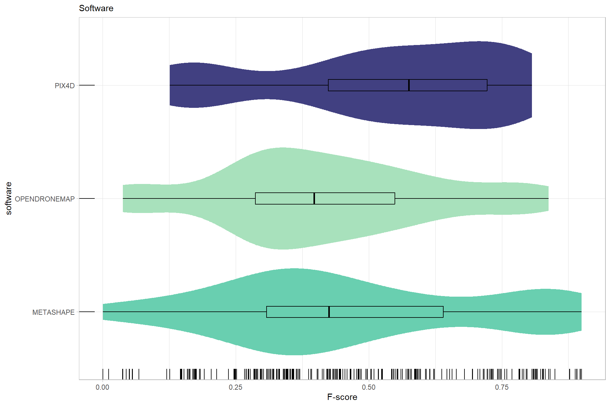
##
## [[2]]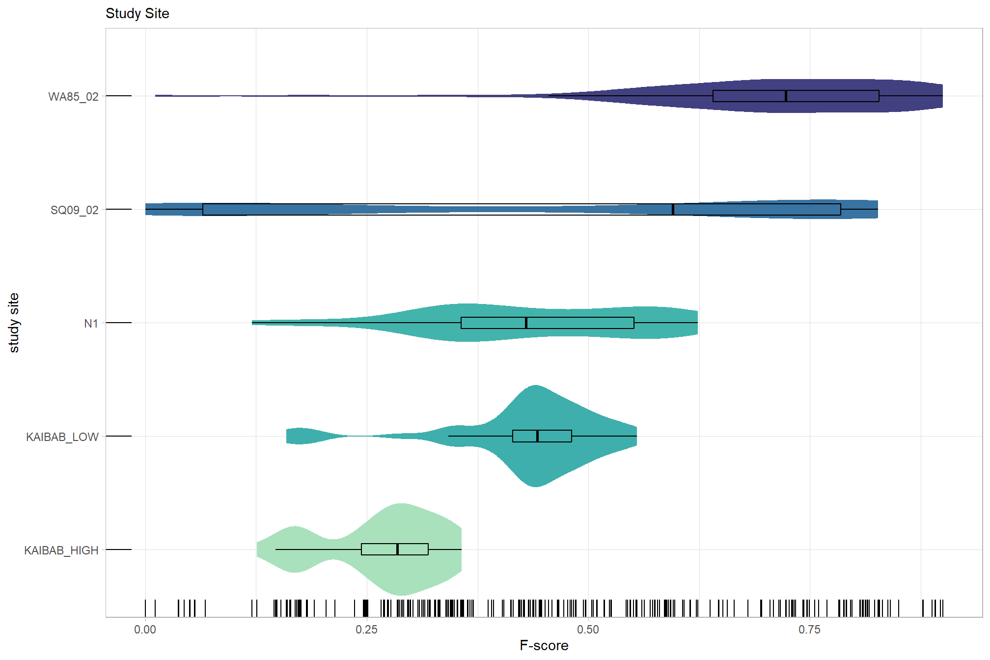
##
## [[3]]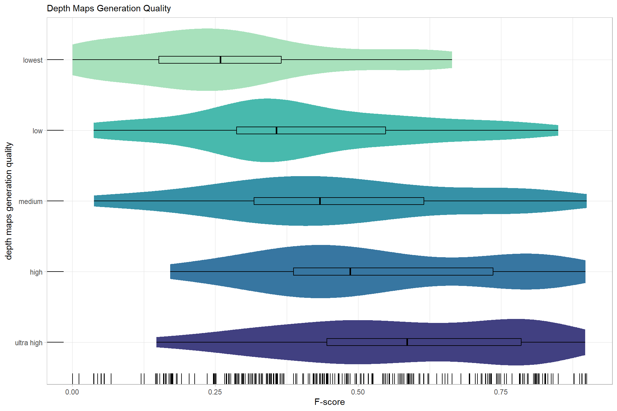
##
## [[4]]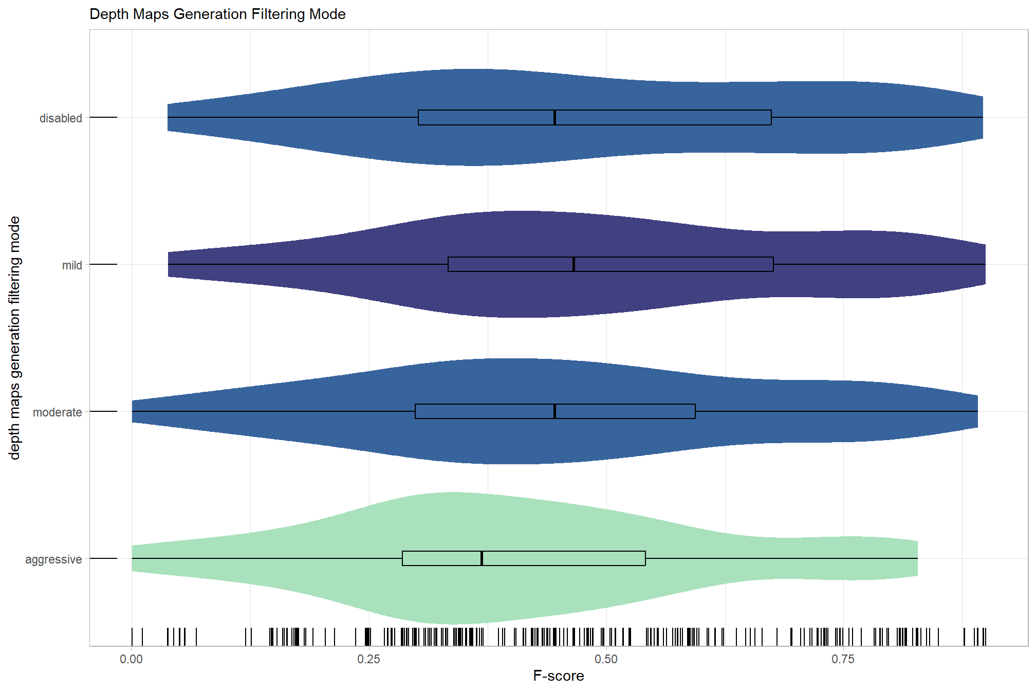
6.3 One Nominal Predictor
We’ll start by exploring the influence of the depth map generation quality parameter on the SfM-derived tree detection performance based on the F-score.
6.3.1 Summary Statistics
Summary statistics by group:
ptcld_validation_data %>%
  dplyr::group_by(depth_maps_generation_quality) %>%
  dplyr::summarise(
    mean_f_score = mean(f_score, na.rm = T)
    # , med_f_score = median(f_score, na.rm = T)
    , sd_f_score = sd(f_score, na.rm = T)
    , n = dplyr::n()
  ) %>%
  kableExtra::kbl(digits = 2, caption = "summary statistics: F-score by dense cloud quality") %>%
kableExtra::kable_styling()| depth_maps_generation_quality | mean_f_score | sd_f_score | n |
|---|---|---|---|
| ultra high | 0.58 | 0.21 | 55 |
| high | 0.54 | 0.21 | 55 |
| medium | 0.47 | 0.22 | 55 |
| low | 0.40 | 0.20 | 55 |
| lowest | 0.27 | 0.19 | 40 |
6.3.2 Bayesian
Kruschke (2015) notes:
The terminology, “analysis of variance,” comes from a decomposition of overall data variance into within-group variance and between-group variance (Fisher, 1925). Algebraically, the sum of squared deviations of the scores from their overall mean equals the sum of squared deviations of the scores from their respective group means plus the sum of squared deviations of the group means from the overall mean. In other words, the total variance can be partitioned into within-group variance plus between-group variance. Because one definition of the word “analysis” is separation into constituent parts, the term ANOVA accurately describes the underlying algebra in the traditional methods. That algebraic relation is not used in the hierarchical Bayesian approach presented here. The Bayesian method can estimate component variances, however. Therefore, the Bayesian approach is not ANOVA, but is analogous to ANOVA. (p. 556)
and see section 19 from Kurz’s ebook supplement
The metric predicted variable with one nominal predictor variable model has the form:
\[\begin{align*} y_{i} &\sim \operatorname{Normal} \bigl(\mu_{i}, \sigma_{y} \bigr) \\ \mu_{i} &= \beta_0 + \sum_{j=1}^{J} \beta_{1[j]} x_{1[j]} \bigl(i\bigr) \\ \beta_{0} &\sim \operatorname{Normal}(0,10) \\ \beta_{1[j]} &\sim \operatorname{Normal}(0,\sigma_{\beta_{1}}) \\ \sigma_{\beta_{1}} &\sim {\sf uniform} (0,100) \\ \sigma_{y} &\sim {\sf uniform} (0,100) \\ \end{align*}\]
, where \(j\) is the depth map generation quality setting corresponding to observation \(i\)
to start, we’ll use the default brms::brm prior settings which may not match those described in the model specification above
brms_f_mod1 = brms::brm(
formula = f_score ~ 1 + (1 | depth_maps_generation_quality)
, data = ptcld_validation_data
, family = brms::brmsfamily(family = "gaussian")
, iter = 4000, warmup = 2000, chains = 4
, cores = round(parallel::detectCores()/2)
, file = paste0(rootdir, "/fits/brms_f_mod1")
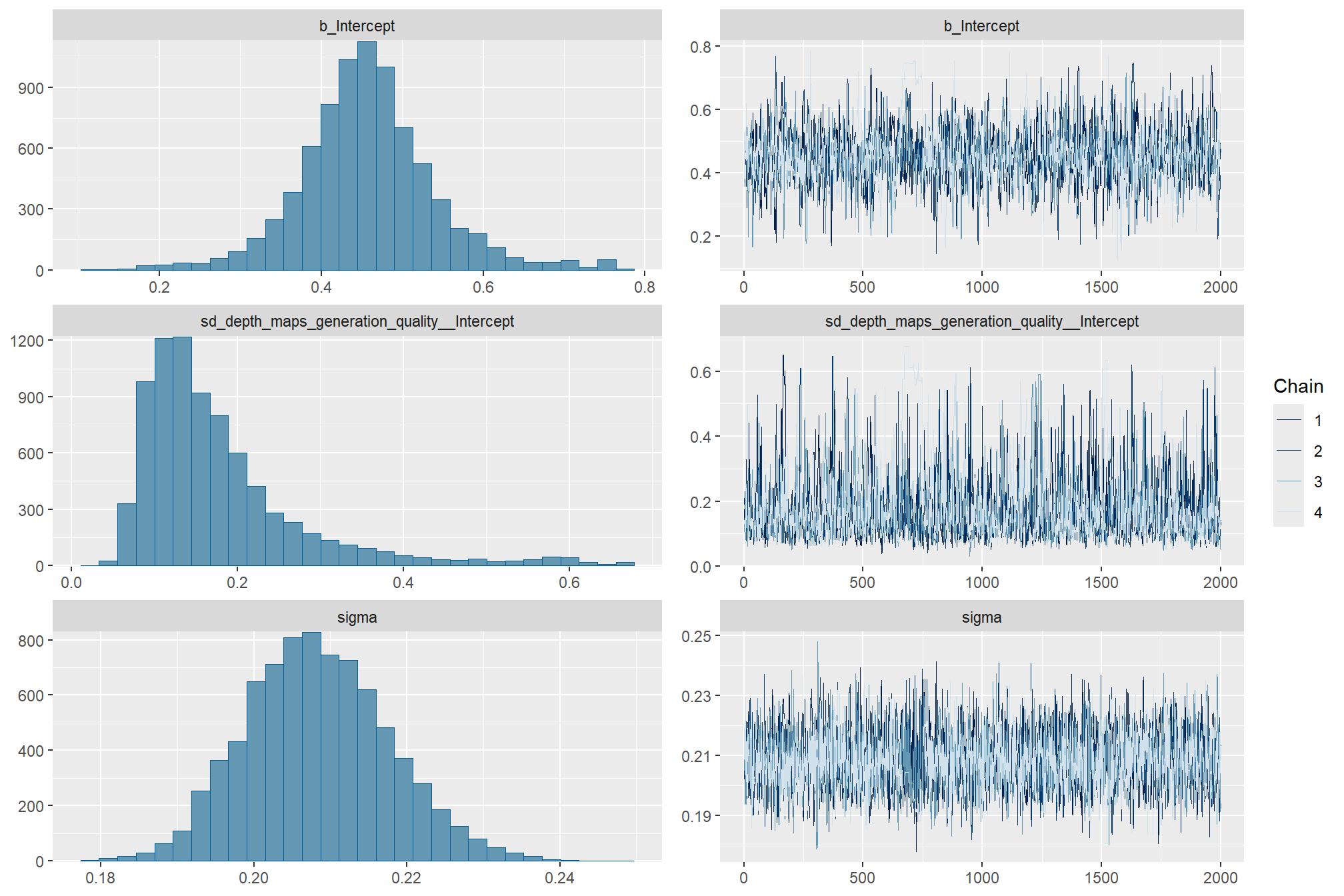
)check the trace plots for problems with convergence of the Markov chains
check the prior distributions
# check priors
brms::prior_summary(brms_f_mod1) %>%
  kableExtra::kbl() %>%
kableExtra::kable_styling()| prior | class | coef | group | resp | dpar | nlpar | lb | ub | source |
|---|---|---|---|---|---|---|---|---|---|
| student_t(3, 0.4, 2.5) | Intercept | default | |||||||
| student_t(3, 0, 2.5) | sd | 0 | default | ||||||
| sd | depth_maps_generation_quality | default | |||||||
| sd | Intercept | depth_maps_generation_quality | default | ||||||
| student_t(3, 0, 2.5) | sigma | 0 | default |
The brms::brm model summary
brms_f_mod1 %>%
  brms::posterior_summary() %>%
  as.data.frame() %>%
  tibble::rownames_to_column(var = "parameter") %>%
  dplyr::rename_with(tolower) %>%
  dplyr::filter(
    stringr::str_starts(parameter, "b_")
    | stringr::str_starts(parameter, "r_")
    | parameter == "sigma"
  ) %>%
  dplyr::mutate(
    parameter = parameter %>%
      stringr::str_remove_all("b_depth_maps_generation_quality") %>%
      stringr::str_remove_all("r_depth_maps_generation_quality")
  ) %>%
  kableExtra::kbl(digits = 2, caption = "Bayesian one nominal predictor: F-score by dense cloud quality") %>%
kableExtra::kable_styling()| parameter | estimate | est.error | q2.5 | q97.5 |
|---|---|---|---|---|
| b_Intercept | 0.46 | 0.08 | 0.29 | 0.65 |
| sigma | 0.21 | 0.01 | 0.19 | 0.23 |
| [ultra.high,Intercept] | 0.11 | 0.09 | -0.08 | 0.29 |
| [high,Intercept] | 0.08 | 0.09 | -0.12 | 0.25 |
| [medium,Intercept] | 0.01 | 0.09 | -0.19 | 0.18 |
| [low,Intercept] | -0.05 | 0.09 | -0.25 | 0.12 |
| [lowest,Intercept] | -0.17 | 0.09 | -0.37 | 0.00 |
With the stats::coef function, we can get the group-level summaries in a “non-deflection” metric. In the model, the group means represented by \(\beta_{1[j]}\) are deflections from overall baseline, such that the deflections sum to zero (see Kruschke (2015, p.554)). Summaries of the group-specific deflections are available via the brms::ranef function.
stats::coef(brms_f_mod1) %>%
  as.data.frame() %>%
  tibble::rownames_to_column(var = "group") %>%
  dplyr::rename_with(
    .cols = -c("group")
    , .fn = ~ stringr::str_remove_all(.x, "depth_maps_generation_quality.")
  ) %>%
  kableExtra::kbl(digits = 2, caption = "brms::brm model: F-score by dense cloud quality") %>%
kableExtra::kable_styling()| group | Estimate.Intercept | Est.Error.Intercept | Q2.5.Intercept | Q97.5.Intercept |
|---|---|---|---|---|
| ultra high | 0.57 | 0.03 | 0.51 | 0.62 |
| high | 0.53 | 0.03 | 0.48 | 0.59 |
| medium | 0.47 | 0.03 | 0.41 | 0.52 |
| low | 0.40 | 0.03 | 0.35 | 0.46 |
| lowest | 0.28 | 0.03 | 0.22 | 0.35 |
We can look at the model noise standard deviation \(\sigma_y\)
# get formula
form_temp = brms_f_mod1$formula$formula[3] %>%
  as.character() %>% get_frmla_text() %>%
  stringr::str_replace_all("depth_maps_generation_quality", "quality") %>%
  stringr::str_replace_all("depth_maps_generation_filtering_mode", "filtering")
# extract the posterior draws
brms::as_draws_df(brms_f_mod1) %>%
# plot
  ggplot(aes(x = sigma, y = 0)) +
  tidybayes::stat_dotsinterval(
    point_interval = median_hdi, .width = .95
    , justification = -0.04
    , shape = 21, point_size = 3
    , quantiles = 100
  ) +
  scale_y_continuous(NULL, breaks = NULL) +
  labs(
    x = latex2exp::TeX("$\\sigma_y$")
    , caption = form_temp
  ) +
  theme_light()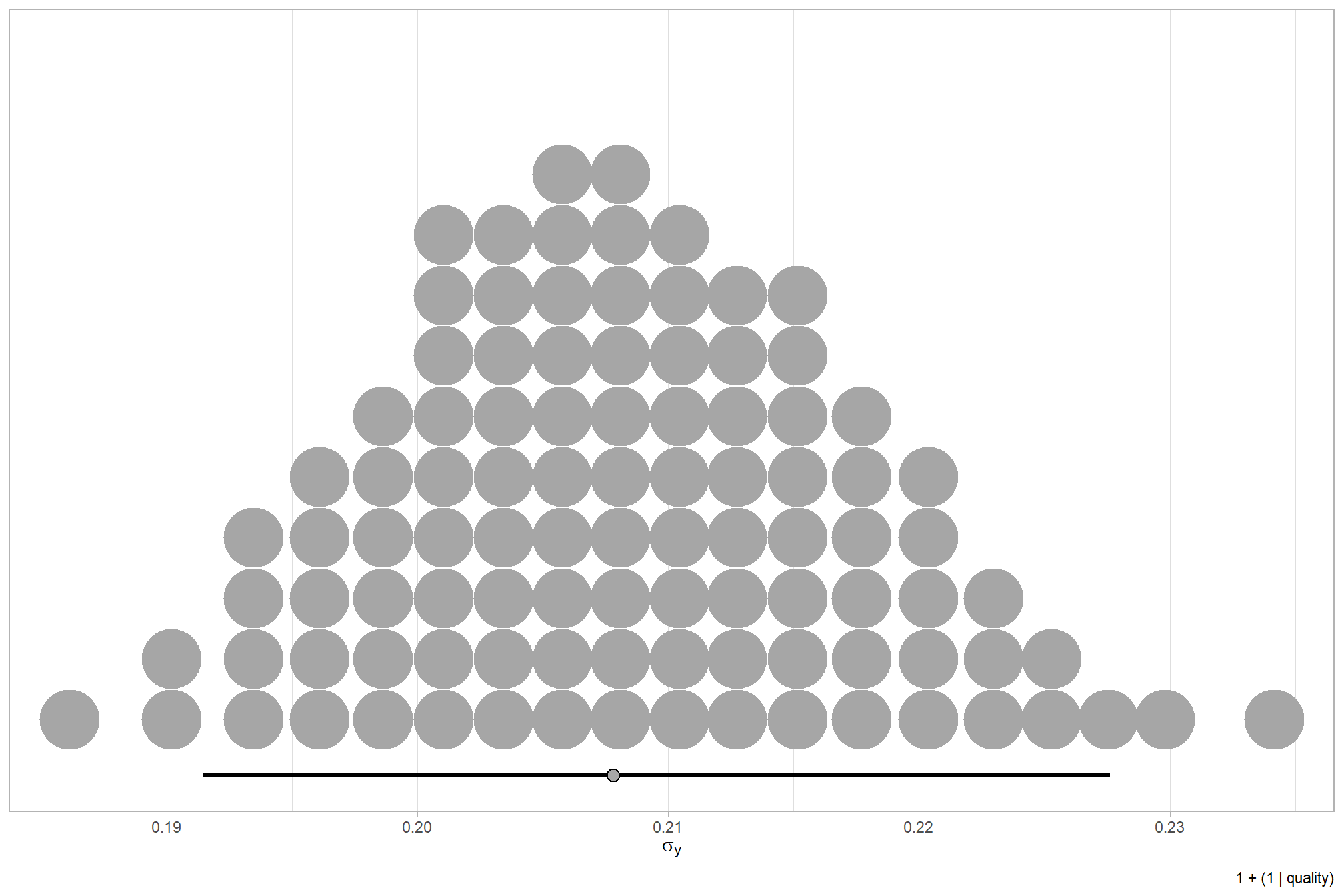
plot the posterior predictive distributions of the conditional means with the median F-score and the 95% highest posterior density interval (HDI)
ptcld_validation_data %>%
  dplyr::distinct(depth_maps_generation_quality) %>%
  tidybayes::add_epred_draws(brms_f_mod1) %>%
  dplyr::mutate(value = .epred) %>%
  # plot
  ggplot(
    mapping = aes(
      x = value, y = depth_maps_generation_quality
      , fill = depth_maps_generation_quality
    )
  ) +
    tidybayes::stat_halfeye(
      point_interval = median_hdi, .width = .95
      , interval_color = "gray66"
      , shape = 21, point_color = "gray66", point_fill = "black"
      , justification = -0.01
    ) +
    scale_fill_viridis_d(option = "inferno", drop = F) +
    scale_x_continuous(breaks = scales::extended_breaks(n=8)) +
    labs(
      y = "quality", x = "F-score"
      , subtitle = "posterior predictive distribution of F-score with 95% HDI"
      , caption = form_temp
    ) +
    theme_light() +
    theme(legend.position = "none")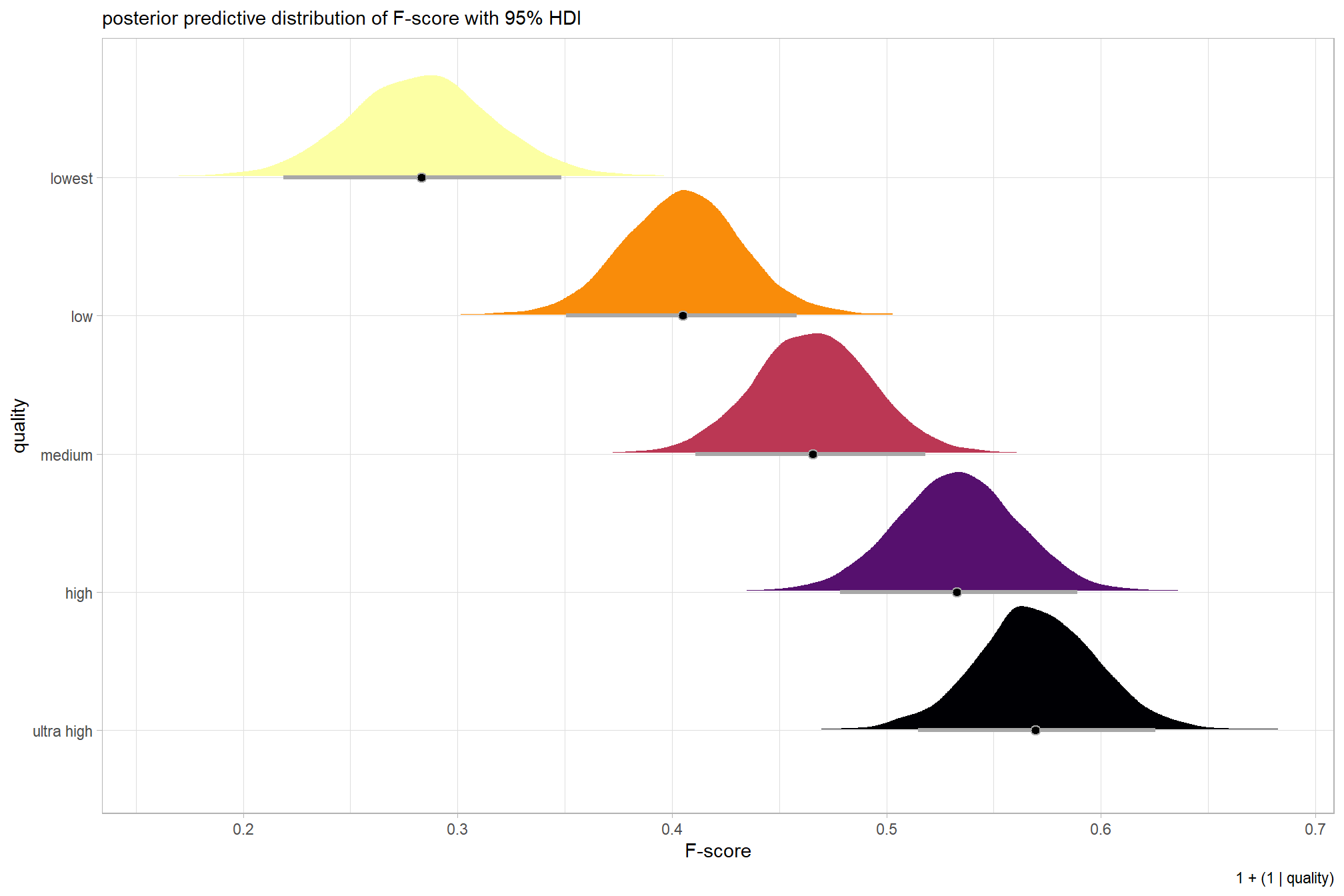
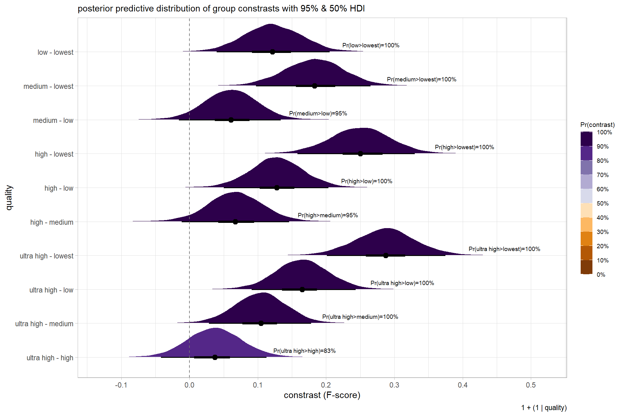
we can also make pairwise comparisons
# first we need to define the contrasts to make
contrast_list =
  tidyr::crossing(
    x1 = unique(ptcld_validation_data$depth_maps_generation_quality)
    , x2 = unique(ptcld_validation_data$depth_maps_generation_quality)
  ) %>%
  dplyr::mutate(
    dplyr::across(
      dplyr::everything()
      , .fns = function(x){factor(
        x, ordered = T
        , levels = levels(ptcld_validation_data$depth_maps_generation_quality)
      )}
    )
  ) %>%
  dplyr::filter(x1<x2) %>%
  dplyr::arrange(x1,x2) %>%
  dplyr::mutate(dplyr::across(dplyr::everything(), as.character)) %>%
  purrr::transpose()

# contrast_list

# obtain posterior draws and calculate contrasts using tidybayes::compare_levels
brms_contrast_temp =
  brms_f_mod1 %>%
    tidybayes::spread_draws(r_depth_maps_generation_quality[depth_maps_generation_quality]) %>%
    dplyr::mutate(
      depth_maps_generation_quality = depth_maps_generation_quality %>%
        stringr::str_replace_all("\\.", " ") %>%
        factor(
          levels = levels(ptcld_validation_data$depth_maps_generation_quality)
          , ordered = T
        )
    ) %>%
    dplyr::rename(value = r_depth_maps_generation_quality) %>%
    tidybayes::compare_levels(
      value
      , by = depth_maps_generation_quality
      , comparison = contrast_list
        # tidybayes::emmeans_comparison("revpairwise")
        #"pairwise"
    )

# generate the contrast column for creating an ordered factor
brms_contrast_temp =
  brms_contrast_temp %>%
  dplyr::ungroup() %>%
  tidyr::separate_wider_delim(
    cols = depth_maps_generation_quality
    , delim = " - "
    , names = paste0(
        "sorter"
        , 1:(max(stringr::str_count(brms_contrast_temp$depth_maps_generation_quality, "-"))+1)
      )
    , too_few = "align_start"
    , cols_remove = F
  ) %>%
  dplyr::filter(sorter1!=sorter2) %>%
  dplyr::mutate(
    dplyr::across(
      tidyselect::starts_with("sorter")
      , .fns = function(x){factor(
        x, ordered = T
        , levels = levels(ptcld_validation_data$depth_maps_generation_quality)
      )}
    )
    , contrast = depth_maps_generation_quality %>% forcats::fct_reorder(
        paste0(as.numeric(sorter1), as.numeric(sorter2)) %>%
        as.numeric()
      )
  )

# median_hdi summary for coloring
brms_contrast_temp = brms_contrast_temp %>%
  dplyr::group_by(contrast) %>%
  dplyr::mutate(
    # get median_hdi
    median_hdi_est = tidybayes::median_hdi(value)$y
    , median_hdi_lower = tidybayes::median_hdi(value)$ymin
    , median_hdi_upper = tidybayes::median_hdi(value)$ymax
    # check probability of contrast
    , pr_gt_zero = mean(value > 0) %>%
        scales::percent(accuracy = 1)
    , pr_lt_zero = mean(value < 0) %>%
        scales::percent(accuracy = 1)
    # check probability that this direction is true
    , is_diff_dir = dplyr::case_when(
      median_hdi_est >= 0 ~ value > 0
      , median_hdi_est < 0 ~ value < 0
    )
    , pr_diff = mean(is_diff_dir)
    # make a label
    , pr_diff_lab = dplyr::case_when(
      median_hdi_est > 0 ~ paste0(
        "Pr("
        , stringr::word(contrast, 1, sep = fixed("-")) %>%
          stringr::str_squish()
        , ">"
        , stringr::word(contrast, 2, sep = fixed("-")) %>%
          stringr::str_squish()
        , ")="
        , pr_diff %>% scales::percent(accuracy = 1)
      )
      , median_hdi_est < 0 ~ paste0(
        "Pr("
        , stringr::word(contrast, 2, sep = fixed("-")) %>%
          stringr::str_squish()
        , ">"
        , stringr::word(contrast, 1, sep = fixed("-")) %>%
          stringr::str_squish()
        , ")="
        , pr_diff %>% scales::percent(accuracy = 1)
      )
    )
    # make a SMALLER label
    , pr_diff_lab_sm = dplyr::case_when(
      median_hdi_est >= 0 ~ paste0(
        "Pr(>0)="
        , pr_diff %>% scales::percent(accuracy = 1)
      )
      , median_hdi_est < 0 ~ paste0(
        "Pr(<0)="
        , pr_diff %>% scales::percent(accuracy = 1)
      )
    )
    , pr_diff_lab_pos = dplyr::case_when(
      median_hdi_est > 0 ~ median_hdi_upper
      , median_hdi_est < 0 ~ median_hdi_lower
    ) * 1.09
    , sig_level = dplyr::case_when(
      pr_diff > 0.99 ~ 0
      , pr_diff > 0.95 ~ 1
      , pr_diff > 0.9 ~ 2
      , pr_diff > 0.8 ~ 3
      , T ~ 4
    ) %>%
    factor(levels = c(0:4), labels = c(">99%","95%","90%","80%","<80%"), ordered = T)
  )
# what?
brms_contrast_temp %>%
  dplyr::ungroup() %>%
  dplyr::count(contrast, median_hdi_est, pr_diff_lab,pr_diff_lab_sm)
## # A tibble: 10 × 5
## contrast median_hdi_est pr_diff_lab pr_diff_lab_sm n
## <fct> <dbl> <chr> <chr> <int>
## 1 ultra high - high 0.0370 Pr(ultra high>high)=… Pr(>0)=83% 8000
## 2 ultra high - medium 0.105 Pr(ultra high>medium… Pr(>0)=100% 8000
## 3 ultra high - low 0.165 Pr(ultra high>low)=1… Pr(>0)=100% 8000
## 4 ultra high - lowest 0.287 Pr(ultra high>lowest… Pr(>0)=100% 8000
## 5 high - medium 0.0670 Pr(high>medium)=95% Pr(>0)=95% 8000
## 6 high - low 0.128 Pr(high>low)=100% Pr(>0)=100% 8000
## 7 high - lowest 0.250 Pr(high>lowest)=100% Pr(>0)=100% 8000
## 8 medium - low 0.0607 Pr(medium>low)=95% Pr(>0)=95% 8000
## 9 medium - lowest 0.183 Pr(medium>lowest)=10… Pr(>0)=100% 8000
## 10 low - lowest 0.121 Pr(low>lowest)=100% Pr(>0)=100% 8000plot it
# plot, finally
brms_contrast_temp %>%
  ggplot(aes(x = value, y = contrast, fill = pr_diff)) +
    tidybayes::stat_halfeye(
      point_interval = median_hdi, .width = c(0.5,0.95)
      # , slab_fill = "gray22", slab_alpha = 1
      , interval_color = "black", point_color = "black", point_fill = "black"
      , justification = -0.01
    ) +
    geom_vline(xintercept = 0, linetype = "dashed", color = "gray44") +
    geom_text(
      data = brms_contrast_temp %>%
        dplyr::ungroup() %>%
        dplyr::count(contrast, pr_diff_lab, pr_diff_lab_pos, pr_diff)
      , mapping = aes(x = pr_diff_lab_pos, label = pr_diff_lab)
      , vjust = -1, hjust = 0, size = 2.5
    ) +
    scale_fill_fermenter(
      n.breaks = 10, palette = "PuOr"
      , direction = 1
      , limits = c(0,1)
      , labels = scales::percent
    ) +
    scale_x_continuous(breaks = scales::extended_breaks(n=8), expand = expansion(mult = c(0.1,0.2))) +
    labs(
      y = "quality"
      , x = "constrast (F-score)"
      , fill = "Pr(contrast)"
      , subtitle = "posterior predictive distribution of group constrasts with 95% & 50% HDI"
      , caption = form_temp
    ) +
    theme_light() +
    theme(
      legend.text = element_text(size = 7)
      , legend.title = element_text(size = 8)
    ) +
    guides(fill = guide_colorbar(theme = theme(
      legend.key.width  = unit(1, "lines"),
      legend.key.height = unit(12, "lines")
    )))
and summarize these contrasts
# # can also use the following as substitute for the "tidybayes::spread_draws" used above to get same result
brms_contrast_temp %>%
  dplyr::group_by(contrast) %>%
  tidybayes::median_hdi(value) %>%
  select(-c(.point,.interval, .width)) %>%
  dplyr::arrange(desc(contrast)) %>%

  kableExtra::kbl(
    digits = 2
    , caption = "brms::brm model: 95% HDI of the posterior predictive distribution of group constrasts in F-score"
    , col.names = c(
      "quality contrast"
      , "difference (F-score)"
      , "HDI low", "HDI high"
    )
  ) %>%
kableExtra::kable_styling()| quality contrast | difference (F-score) | HDI low | HDI high |
|---|---|---|---|
| low - lowest | 0.12 | 0.04 | 0.21 |
| medium - lowest | 0.18 | 0.10 | 0.27 |
| medium - low | 0.06 | -0.02 | 0.13 |
| high - lowest | 0.25 | 0.16 | 0.33 |
| high - low | 0.13 | 0.05 | 0.20 |
| high - medium | 0.07 | -0.01 | 0.15 |
| ultra high - lowest | 0.29 | 0.20 | 0.37 |
| ultra high - low | 0.16 | 0.09 | 0.24 |
| ultra high - medium | 0.10 | 0.03 | 0.18 |
| ultra high - high | 0.04 | -0.04 | 0.11 |
Before we move on to the next section, look above at how many arguments we fiddled with to configure our tidybayes::stat_halfeye() plot. Given how many more contrast plots we have looming in our not-too-distant future, we might go ahead and save these settings as a new function. We’ll call it plt_contrast().
plt_contrast <- function(
    my_data
    , x = "value"
    , y = "contrast"
    , fill = "pr_diff"
    , label = "pr_diff_lab"
    , label_pos = "pr_diff_lab_pos"
    , label_size = 3
    , x_expand = c(0.1, 0.1)
    , facet = NA
    , y_axis_title = ""
    , caption_text = "" # form_temp
    , annotate_size = 2.2
    ) {
  # df for annotation
  get_annotation_df <- function(
        my_text_list = c(
          "Bottom Left (h0,v0)","Top Left (h0,v1)"
          ,"Bottom Right h1,v0","Top Right h1,v1"
          )
        , hjust = c(0,0,1,1) # higher values = right, lower values = left
        , vjust = c(0,1.3,0,1.3) # higher values = down, lower values = up
    ){
      df = data.frame(
        xpos = c(-Inf,-Inf,Inf,Inf)
        , ypos =  c(-Inf, Inf,-Inf,Inf)
        , annotate_text = my_text_list
        , hjustvar = hjust
        , vjustvar = vjust
      )
      return(df)
  }
  # plot
  plt =
    my_data %>%
    ggplot(aes(x = .data[[x]], y = .data[[y]])) +
      geom_vline(xintercept = 0, linetype = "solid", color = "gray33", lwd = 1.1) +
      tidybayes::stat_halfeye(
        mapping = aes(fill = .data[[fill]])
        , point_interval = median_hdi, .width = c(0.5,0.95)
        # , slab_fill = "gray22", slab_alpha = 1
        , interval_color = "black", point_color = "black", point_fill = "black"
        , point_size = 0.9
        , justification = -0.01
      ) +
      geom_text(
        data = get_annotation_df(
          my_text_list = c(
          "","L.H.S. < R.H.S."
          ,"","L.H.S. > R.H.S."
          )
        )
        , mapping = aes(
          x = xpos, y = ypos
          , hjust = hjustvar, vjust = vjustvar
          , label = annotate_text
          , fontface = "bold"
        )
        , size = annotate_size
        , color = "gray30" # "#2d2a4d" #"#204445"
      ) +
      # scale_fill_fermenter(
      #   n.breaks = 5 # 10 use 10 if can go full range 0-1
      #   , palette = "PuOr" # "RdYlBu"
      #   , direction = 1
      #   , limits = c(0.5,1) # use c(0,1) if can go full range 0-1
      #   , labels = scales::percent
      # ) +
      scale_fill_stepsn(
        n.breaks = 5 # 10 use 10 if can go full range 0-1
        , colors = RColorBrewer::brewer.pal(11,"PuOr")[c(3,4,8,10,11)]
        , limits = c(0.5,1) # use c(0,1) if can go full range 0-1
        , labels = scales::percent
      ) +
      scale_x_continuous(expand = expansion(mult = x_expand)) +
      labs(
        y = y_axis_title
        , x = "constrast (F-score)"
        , fill = "Pr(contrast)"
        , subtitle = "posterior predictive distribution of group constrasts with 95% & 50% HDI"
        , caption = caption_text
      ) +
      theme_light() +
      theme(
        legend.text = element_text(size = 7)
        , legend.title = element_text(size = 8)
        , axis.text.x = element_text(angle = 90, vjust = 0.5, hjust = 1.05)
        , strip.text = element_text(color = "black", face = "bold")
      ) +
      guides(fill = guide_colorbar(theme = theme(
        legend.key.width  = unit(1, "lines"),
        legend.key.height = unit(12, "lines")
      )))
  # return facet or not
  if(max(is.na(facet))==0){
    return(
      plt +
        geom_text(
          data = my_data %>%
            dplyr::filter(pr_diff_lab_pos>=0) %>%
            dplyr::ungroup() %>%
            dplyr::select(tidyselect::all_of(c(
              y
              , fill
              , label
              , label_pos
              , facet
            ))) %>%
            dplyr::distinct()
          , mapping = aes(x = .data[[label_pos]], label = .data[[label]])
          , vjust = -1, hjust = 0, size = label_size
        ) +
        geom_text(
          data = my_data %>%
            dplyr::filter(pr_diff_lab_pos<0) %>%
            dplyr::ungroup() %>%
            dplyr::select(tidyselect::all_of(c(
              y
              , fill
              , label
              , label_pos
              , facet
            ))) %>%
            dplyr::distinct()
          , mapping = aes(x = .data[[label_pos]], label = .data[[label]])
          , vjust = -1, hjust = +1, size = label_size
        ) +
        facet_grid(cols = vars(.data[[facet]]))

    )
  }
  else{
    return(
      plt +
        geom_text(
          data = my_data %>%
            dplyr::filter(pr_diff_lab_pos>=0) %>%
            dplyr::ungroup() %>%
            dplyr::select(tidyselect::all_of(c(
              y
              , fill
              , label
              , label_pos
            ))) %>%
            dplyr::distinct()
          , mapping = aes(x = .data[[label_pos]], label = .data[[label]])
          , vjust = -1, hjust = 0, size = label_size
        )+
        geom_text(
          data = my_data %>%
            dplyr::filter(pr_diff_lab_pos<0) %>%
            dplyr::ungroup() %>%
            dplyr::select(tidyselect::all_of(c(
              y
              , fill
              , label
              , label_pos
            ))) %>%
            dplyr::distinct()
          , mapping = aes(x = .data[[label_pos]], label = .data[[label]])
          , vjust = -1, hjust = +1, size = label_size
        )
    )
  }
}
# plt_contrast(brms_contrast_temp, label = "pr_diff_lab_sm")
We’ll also create a function to create all of the probability labeling columns in the contrast data called make_contrast_vars()
Note, here we use tidybayes::median_hdci() to avoid potential for returning multiple rows by group if our data is grouped. See the documentation for the ggdist package which notes that “If the distribution is multimodal, hdi may return multiple intervals for each probability level (these will be spread over rows).”
make_contrast_vars = function(my_data){
  my_data %>%
    dplyr::mutate(
      # get median_hdi
      median_hdi_est = tidybayes::median_hdci(value)$y
      , median_hdi_lower = tidybayes::median_hdci(value)$ymin
      , median_hdi_upper = tidybayes::median_hdci(value)$ymax
      # check probability of contrast
      , pr_gt_zero = mean(value > 0) %>%
          scales::percent(accuracy = 1)
      , pr_lt_zero = mean(value < 0) %>%
          scales::percent(accuracy = 1)
      # check probability that this direction is true
      , is_diff_dir = dplyr::case_when(
        median_hdi_est >= 0 ~ value > 0
        , median_hdi_est < 0 ~ value < 0
      )
      , pr_diff = mean(is_diff_dir)
      # make a label
      , pr_diff_lab = dplyr::case_when(
          median_hdi_est > 0 ~ paste0(
            "Pr("
            , stringr::word(contrast, 1, sep = fixed("-")) %>%
              stringr::str_squish()
            , ">"
            , stringr::word(contrast, 2, sep = fixed("-")) %>%
              stringr::str_squish()
            , ")="
            , pr_diff %>% scales::percent(accuracy = 1)
          )
          , median_hdi_est < 0 ~ paste0(
            "Pr("
            , stringr::word(contrast, 2, sep = fixed("-")) %>%
              stringr::str_squish()
            , ">"
            , stringr::word(contrast, 1, sep = fixed("-")) %>%
              stringr::str_squish()
            , ")="
            , pr_diff %>% scales::percent(accuracy = 1)
          )
        ) %>%
        stringr::str_replace_all("OPENDRONEMAP", "ODM") %>%
        stringr::str_replace_all("METASHAPE", "MtaShp") %>%
        stringr::str_replace_all("PIX4D", "Pix4D")
      # make a SMALLER label
      , pr_diff_lab_sm = dplyr::case_when(
        median_hdi_est >= 0 ~ paste0(
          "Pr(>0)="
          , pr_diff %>% scales::percent(accuracy = 1)
        )
        , median_hdi_est < 0 ~ paste0(
          "Pr(<0)="
          , pr_diff %>% scales::percent(accuracy = 1)
        )
      )
      , pr_diff_lab_pos = dplyr::case_when(
        median_hdi_est > 0 ~ median_hdi_upper
        , median_hdi_est < 0 ~ median_hdi_lower
      ) * 1.075
      , sig_level = dplyr::case_when(
        pr_diff > 0.99 ~ 0
        , pr_diff > 0.95 ~ 1
        , pr_diff > 0.9 ~ 2
        , pr_diff > 0.8 ~ 3
        , T ~ 4
      ) %>%
      factor(levels = c(0:4), labels = c(">99%","95%","90%","80%","<80%"), ordered = T)
    )
}
# brms_contrast_temp %>% dplyr::group_by(contrast) %>% make_contrast_vars() %>% dplyr::glimpse()
6.4 Two Nominal Predictors
Now, we’ll determine the combined influence of the depth map generation quality and the depth map filtering parameters on the SfM-derived tree detection performance based on the F-score.
6.4.1 Summary Statistics
Summary statistics by group:
ptcld_validation_data %>%
  dplyr::group_by(depth_maps_generation_quality, depth_maps_generation_filtering_mode) %>%
  dplyr::summarise(
    mean_f_score = mean(f_score, na.rm = T)
    # , med_f_score = median(f_score, na.rm = T)
    , sd_f_score = sd(f_score, na.rm = T)
    , n = dplyr::n()
  ) %>%
  kableExtra::kbl(
    digits = 2
    , caption = "summary statistics: F-score by dense cloud quality and filtering mode"
    , col.names = c(
      "quality"
      , "filtering mode"
      , "mean F-score"
      , "sd"
      , "n"
    )
  ) %>%
  kableExtra::kable_styling() %>%
kableExtra::scroll_box(height = "6in")| quality | filtering mode | mean F-score | sd | n |
|---|---|---|---|---|
| ultra high | aggressive | 0.58 | 0.20 | 10 |
| ultra high | moderate | 0.58 | 0.21 | 15 |
| ultra high | mild | 0.58 | 0.21 | 15 |
| ultra high | disabled | 0.56 | 0.23 | 15 |
| high | aggressive | 0.52 | 0.17 | 10 |
| high | moderate | 0.54 | 0.22 | 15 |
| high | mild | 0.54 | 0.22 | 15 |
| high | disabled | 0.54 | 0.23 | 15 |
| medium | aggressive | 0.39 | 0.16 | 10 |
| medium | moderate | 0.47 | 0.22 | 15 |
| medium | mild | 0.50 | 0.25 | 15 |
| medium | disabled | 0.48 | 0.25 | 15 |
| low | aggressive | 0.30 | 0.13 | 10 |
| low | moderate | 0.37 | 0.18 | 15 |
| low | mild | 0.46 | 0.22 | 15 |
| low | disabled | 0.45 | 0.23 | 15 |
| lowest | aggressive | 0.24 | 0.18 | 10 |
| lowest | moderate | 0.25 | 0.20 | 10 |
| lowest | mild | 0.30 | 0.18 | 10 |
| lowest | disabled | 0.30 | 0.21 | 10 |
6.4.2 Bayesian
Kruschke (2015) describes the Hierarchical Bayesian approach to describe groups of metric data with multiple nominal predictors:
This chapter considers data structures that consist of a metric predicted variable and two (or more) nominal predictors….The traditional treatment of this sort of data structure is called multifactor analysis of variance (ANOVA). Our Bayesian approach will be a hierarchical generalization of the traditional ANOVA model. The chapter also considers generalizations of the traditional models, because it is straight forward in Bayesian software to implement heavy-tailed distributions to accommodate outliers, along with hierarchical structure to accommodate heterogeneous variances in the different groups. (pp. 583–584)
and see section 20 from Kurz’s ebook supplement
The metric predicted variable with two nominal predictor variables model has the form:
\[\begin{align*} y_{i} &\sim \operatorname{Normal} \bigl(\mu_{i}, \sigma_{y} \bigr) \\ \mu_{i} &= \beta_0 + \sum_{j} \beta_{1[j]} x_{1[j]} + \sum_{k} \beta_{2[k]} x_{2[k]} + \sum_{j,k} \beta_{1\times2[j,k]} x_{1\times2[j,k]} \\ \beta_{0} &\sim \operatorname{Normal}(0,100) \\ \beta_{1[j]} &\sim \operatorname{Normal}(0,\sigma_{\beta_{1}}) \\ \beta_{2[k]} &\sim \operatorname{Normal}(0,\sigma_{\beta_{2}}) \\ \beta_{1\times2[j,k]} &\sim \operatorname{Normal}(0,\sigma_{\beta_{1\times2}}) \\ \sigma_{\beta_{1}} &\sim \operatorname{Gamma}(1.28,0.005) \\ \sigma_{\beta_{2}} &\sim \operatorname{Gamma}(1.28,0.005) \\ \sigma_{\beta_{1\times2}} &\sim \operatorname{Gamma}(1.28,0.005) \\ \sigma_{y} &\sim {\sf Cauchy} (0,109) \\ \end{align*}\]
, where \(j\) is the depth map generation quality setting corresponding to observation \(i\) and \(k\) is the depth map filtering mode setting corresponding to observation \(i\)
for this model, we’ll define the priors following Kurz who notes that:
The noise standard deviation \(\sigma_y\) is depicted in the prior statement including the argument
class = sigma…in order to be weakly informative, we will use the half-Cauchy. Recall that since the brms default is to set the lower bound for any variance parameter to 0, there’s no need to worry about doing so ourselves. So even though the syntax only indicatescauchy, it’s understood to mean Cauchy with a lower bound at zero; since the mean is usually 0, that makes this a half-Cauchy…The tails of the half-Cauchy are sufficiently fat that, in practice, I’ve found it doesn’t matter much what you set the \(SD\) of its prior to.
# from Kurz:
gamma_a_b_from_omega_sigma = function(mode, sd) {
  if (mode <= 0) stop("mode must be > 0")
  if (sd   <= 0) stop("sd must be > 0")
  rate = (mode + sqrt(mode^2 + 4 * sd^2)) / (2 * sd^2)
  shape = 1 + mode * rate
  return(list(shape = shape, rate = rate))
}

mean_y_temp = mean(ptcld_validation_data$f_score)
sd_y_temp   = sd(ptcld_validation_data$f_score)

omega_temp = sd_y_temp / 2
sigma_temp = 2 * sd_y_temp

s_r_temp = gamma_a_b_from_omega_sigma(mode = omega_temp, sd = sigma_temp)

stanvars_temp =
  brms::stanvar(mean_y_temp,    name = "mean_y") +
  brms::stanvar(sd_y_temp,      name = "sd_y") +
  brms::stanvar(s_r_temp$shape, name = "alpha") +
  brms::stanvar(s_r_temp$rate,  name = "beta")
Now fit the model.
brms_f_mod2 = brms::brm(
formula = f_score ~ 1 +
(1 | depth_maps_generation_quality) +
(1 | depth_maps_generation_filtering_mode) +
(1 | depth_maps_generation_quality:depth_maps_generation_filtering_mode)
, data = ptcld_validation_data
, family = brms::brmsfamily(family = "gaussian")
, iter = 6000, warmup = 3000, chains = 4
, cores = round(parallel::detectCores()/2)
, prior = c(
brms::prior(normal(mean_y, sd_y * 5), class = "Intercept")
, brms::prior(gamma(alpha, beta), class = "sd")
, brms::prior(cauchy(0, sd_y), class = "sigma")
)
, stanvars = stanvars_temp
, file = paste0(rootdir, "/fits/brms_f_mod2")
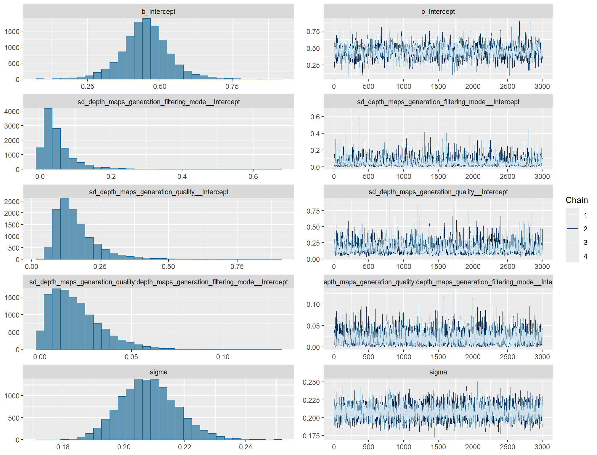
)check the trace plots for problems with convergence of the Markov chains
check the prior distributions
# check priors
brms::prior_summary(brms_f_mod2) %>%
  kableExtra::kbl() %>%
kableExtra::kable_styling()| prior | class | coef | group | resp | dpar | nlpar | lb | ub | source |
|---|---|---|---|---|---|---|---|---|---|
| normal(mean_y, sd_y * 5) | Intercept | user | |||||||
| gamma(alpha, beta) | sd | 0 | user | ||||||
| sd | depth_maps_generation_filtering_mode | default | |||||||
| sd | Intercept | depth_maps_generation_filtering_mode | default | ||||||
| sd | depth_maps_generation_quality | default | |||||||
| sd | Intercept | depth_maps_generation_quality | default | ||||||
| sd | depth_maps_generation_quality:depth_maps_generation_filtering_mode | default | |||||||
| sd | Intercept | depth_maps_generation_quality:depth_maps_generation_filtering_mode | default | ||||||
| cauchy(0, sd_y) | sigma | 0 | user |
The brms::brm model summary
brms_f_mod2 %>%
  brms::posterior_summary() %>%
  as.data.frame() %>%
  tibble::rownames_to_column(var = "parameter") %>%
  dplyr::rename_with(tolower) %>%
  dplyr::filter(
    stringr::str_starts(parameter, "b_")
    | stringr::str_starts(parameter, "r_")
    | stringr::str_starts(parameter, "sd_")
    | parameter == "sigma"
  ) %>%
  dplyr::mutate(
    parameter = parameter %>%
      stringr::str_replace_all("depth_maps_generation_quality", "quality") %>%
      stringr::str_replace_all("depth_maps_generation_filtering_mode", "filtering")
  ) %>%
  kableExtra::kbl(digits = 2, caption = "Bayesian two nominal predictors: F-score by dense cloud quality and filtering mode") %>%
  kableExtra::kable_styling() %>%
kableExtra::scroll_box(height = "6in")| parameter | estimate | est.error | q2.5 | q97.5 |
|---|---|---|---|---|
| b_Intercept | 0.45 | 0.09 | 0.27 | 0.63 |
| sd_filtering__Intercept | 0.05 | 0.05 | 0.00 | 0.19 |
| sd_quality__Intercept | 0.16 | 0.08 | 0.07 | 0.39 |
| sd_quality:filtering__Intercept | 0.02 | 0.01 | 0.00 | 0.05 |
| sigma | 0.21 | 0.01 | 0.19 | 0.23 |
| r_filtering[aggressive,Intercept] | -0.02 | 0.04 | -0.12 | 0.05 |
| r_filtering[moderate,Intercept] | 0.00 | 0.04 | -0.08 | 0.08 |
| r_filtering[mild,Intercept] | 0.02 | 0.04 | -0.05 | 0.11 |
| r_filtering[disabled,Intercept] | 0.01 | 0.04 | -0.06 | 0.10 |
| r_quality[ultra.high,Intercept] | 0.12 | 0.08 | -0.05 | 0.29 |
| r_quality[high,Intercept] | 0.08 | 0.08 | -0.09 | 0.25 |
| r_quality[medium,Intercept] | 0.01 | 0.08 | -0.15 | 0.18 |
| r_quality[low,Intercept] | -0.05 | 0.08 | -0.22 | 0.12 |
| r_quality[lowest,Intercept] | -0.17 | 0.08 | -0.34 | 0.00 |
| r_quality:filtering[high_aggressive,Intercept] | 0.00 | 0.02 | -0.04 | 0.05 |
| r_quality:filtering[high_disabled,Intercept] | 0.00 | 0.02 | -0.05 | 0.05 |
| r_quality:filtering[high_mild,Intercept] | 0.00 | 0.02 | -0.04 | 0.05 |
| r_quality:filtering[high_moderate,Intercept] | 0.00 | 0.02 | -0.04 | 0.05 |
| r_quality:filtering[low_aggressive,Intercept] | -0.01 | 0.02 | -0.07 | 0.03 |
| r_quality:filtering[low_disabled,Intercept] | 0.00 | 0.02 | -0.04 | 0.06 |
| r_quality:filtering[low_mild,Intercept] | 0.01 | 0.02 | -0.04 | 0.06 |
| r_quality:filtering[low_moderate,Intercept] | 0.00 | 0.02 | -0.05 | 0.04 |
| r_quality:filtering[lowest_aggressive,Intercept] | 0.00 | 0.02 | -0.05 | 0.04 |
| r_quality:filtering[lowest_disabled,Intercept] | 0.00 | 0.02 | -0.05 | 0.05 |
| r_quality:filtering[lowest_mild,Intercept] | 0.00 | 0.02 | -0.05 | 0.05 |
| r_quality:filtering[lowest_moderate,Intercept] | 0.00 | 0.02 | -0.06 | 0.04 |
| r_quality:filtering[medium_aggressive,Intercept] | -0.01 | 0.02 | -0.06 | 0.04 |
| r_quality:filtering[medium_disabled,Intercept] | 0.00 | 0.02 | -0.04 | 0.05 |
| r_quality:filtering[medium_mild,Intercept] | 0.00 | 0.02 | -0.04 | 0.05 |
| r_quality:filtering[medium_moderate,Intercept] | 0.00 | 0.02 | -0.04 | 0.05 |
| r_quality:filtering[ultra.high_aggressive,Intercept] | 0.00 | 0.02 | -0.04 | 0.06 |
| r_quality:filtering[ultra.high_disabled,Intercept] | 0.00 | 0.02 | -0.05 | 0.04 |
| r_quality:filtering[ultra.high_mild,Intercept] | 0.00 | 0.02 | -0.05 | 0.05 |
| r_quality:filtering[ultra.high_moderate,Intercept] | 0.00 | 0.02 | -0.04 | 0.05 |
We can look at the model noise standard deviation \(\sigma_y\)
# get formula
form_temp = brms_f_mod2$formula$formula[3] %>%
  as.character() %>% get_frmla_text() %>%
  stringr::str_replace_all("depth_maps_generation_quality", "quality") %>%
  stringr::str_replace_all("depth_maps_generation_filtering_mode", "filtering")
# extract the posterior draws
brms::as_draws_df(brms_f_mod2) %>%
# plot
  ggplot(aes(x = sigma, y = 0)) +
  tidybayes::stat_dotsinterval(
    point_interval = median_hdi, .width = .95
    , justification = -0.04
    , shape = 21, point_size = 3
    , quantiles = 100
  ) +
  scale_y_continuous(NULL, breaks = NULL) +
  labs(
    x = latex2exp::TeX("$\\sigma_y$")
    , caption = form_temp
  ) +
  theme_light()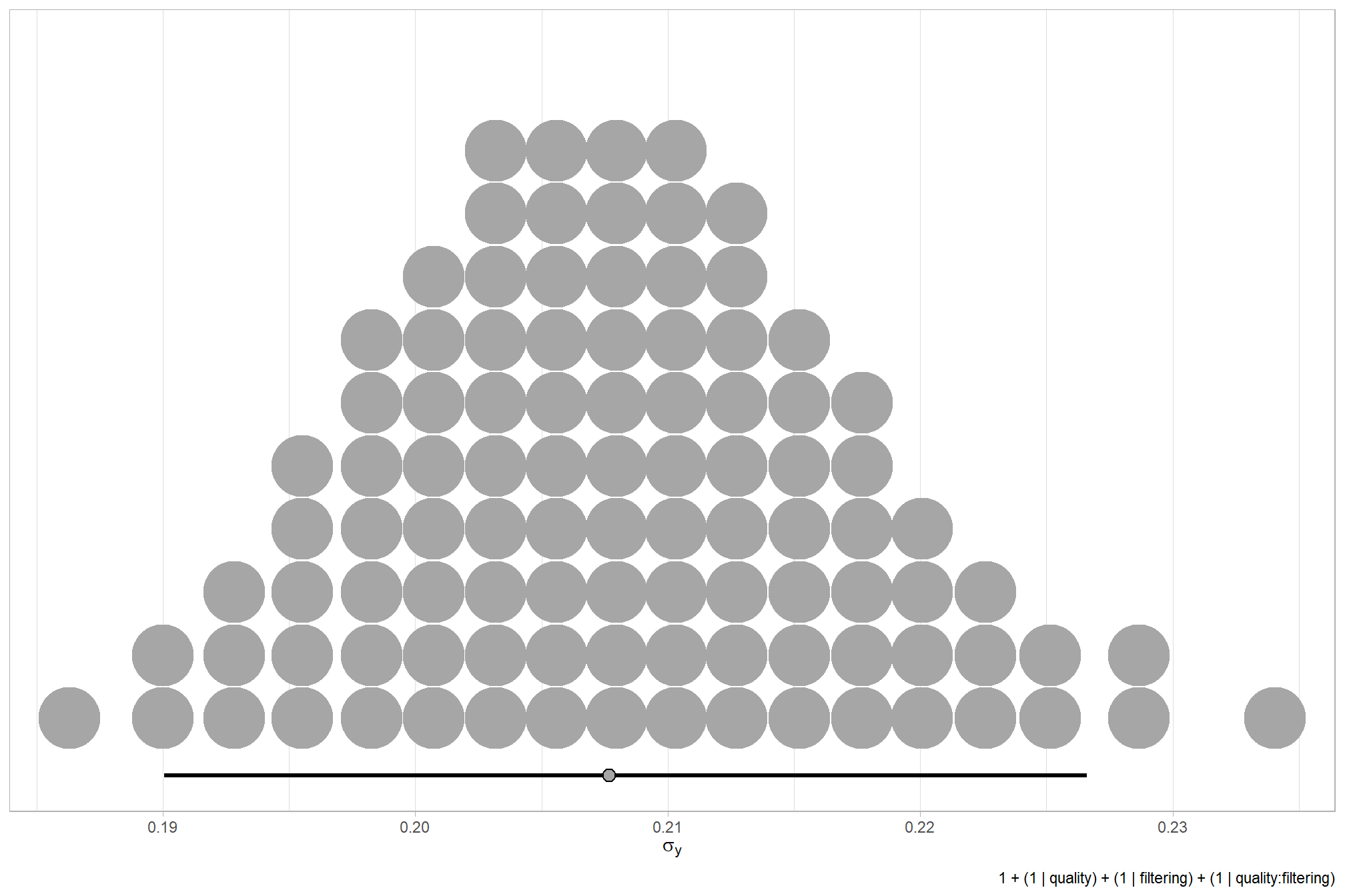
how is it compared to the first model?
# how is it compared to the first model
dplyr::bind_rows(
    brms::as_draws_df(brms_f_mod1) %>% tidybayes::median_hdi(sigma) %>% dplyr::mutate(model = "one nominal predictor")
    , brms::as_draws_df(brms_f_mod2) %>% tidybayes::median_hdi(sigma) %>% dplyr::mutate(model = "two nominal predictor")
  ) %>%
  dplyr::relocate(model) %>%
  kableExtra::kbl(digits = 2, caption = "brms::brm model noise standard deviation comparison") %>%
kableExtra::kable_styling()| model | sigma | .lower | .upper | .width | .point | .interval |
|---|---|---|---|---|---|---|
| one nominal predictor | 0.21 | 0.19 | 0.23 | 0.95 | median | hdi |
| two nominal predictor | 0.21 | 0.19 | 0.23 | 0.95 | median | hdi |
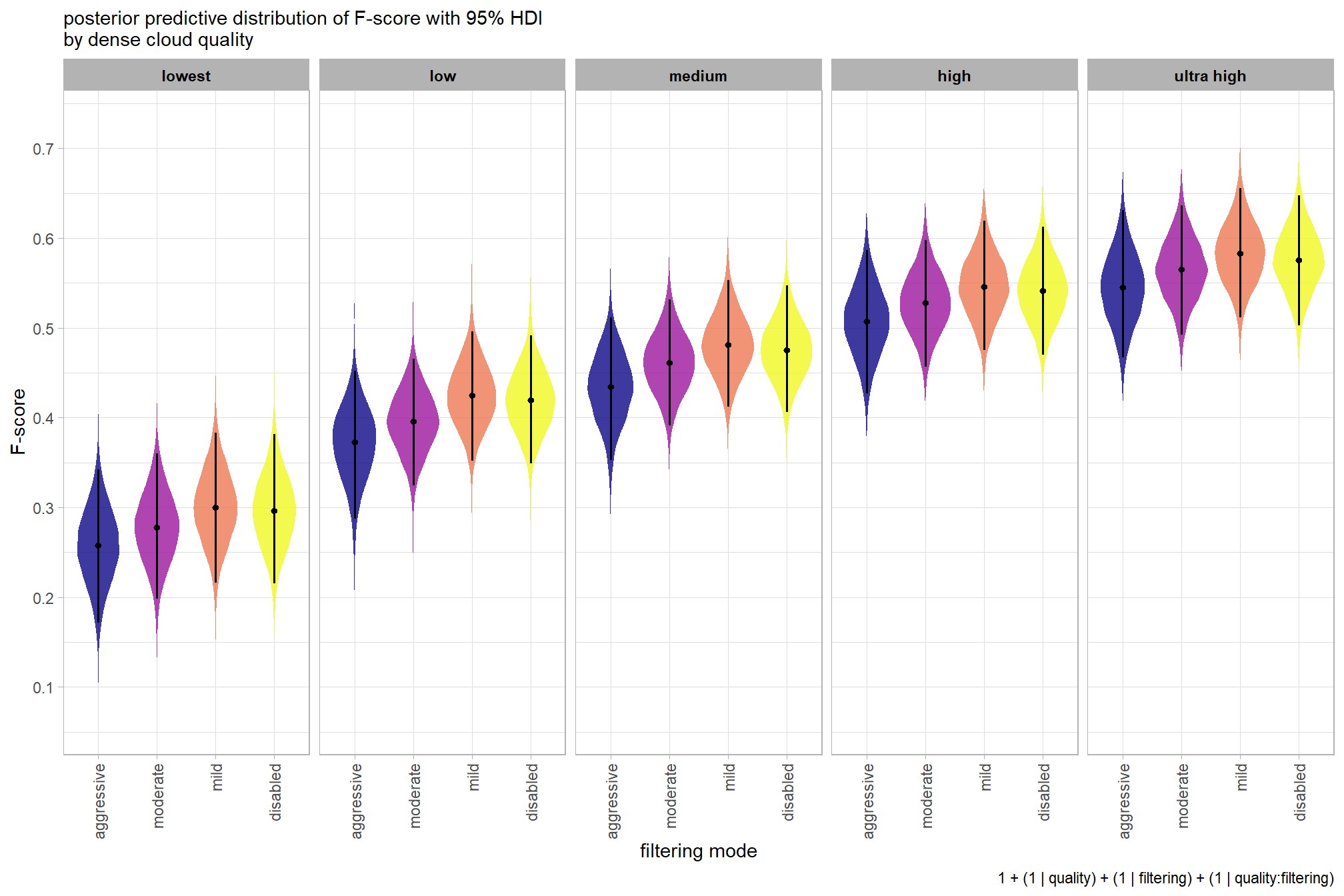
plot the posterior predictive distributions of the conditional means with the median F-score and the 95% highest posterior density interval (HDI)
ptcld_validation_data %>%
  dplyr::distinct(depth_maps_generation_quality, depth_maps_generation_filtering_mode) %>%
  tidybayes::add_epred_draws(brms_f_mod2, allow_new_levels = T) %>%
  dplyr::rename(value = .epred) %>%
  dplyr::mutate(depth_maps_generation_quality = depth_maps_generation_quality %>% forcats::fct_rev()) %>%
  # plot
  ggplot(
    mapping = aes(
      y = value, x = depth_maps_generation_filtering_mode
      , fill = depth_maps_generation_filtering_mode
    )
  ) +
    tidybayes::stat_eye(
      point_interval = median_hdi, .width = .95
      , slab_alpha = 0.8
      , interval_color = "black", linewidth = 1
      , point_color = "black", point_fill = "black", point_size = 1
    ) +
    scale_fill_viridis_d(option = "plasma", drop = F) +
    scale_y_continuous(breaks = scales::extended_breaks(n=10)) +
    facet_grid(cols = vars(depth_maps_generation_quality)) +
    labs(
      x = "filtering mode", y = "F-score"
      , subtitle = "posterior predictive distribution of F-score with 95% HDI\nby dense cloud quality"
      , fill = "Filtering Mode"
      , caption = form_temp
    ) +
    theme_light() +
    theme(
      legend.position = "none"
      , legend.direction  = "horizontal"
      , axis.text.x = element_text(angle = 90, vjust = 0.5, hjust = 1)
      , strip.text = element_text(color = "black", face = "bold")
) 
we can also make pairwise comparisons
brms_contrast_temp =
  ptcld_validation_data %>%
    dplyr::distinct(depth_maps_generation_quality, depth_maps_generation_filtering_mode) %>%
    tidybayes::add_epred_draws(brms_f_mod2, allow_new_levels = T) %>%
    dplyr::rename(value = .epred) %>%
    tidybayes::compare_levels(
      value
      , by = depth_maps_generation_quality
      , comparison =
        contrast_list
        # tidybayes::emmeans_comparison("revpairwise")
        #"pairwise"
    ) %>%
    dplyr::rename(contrast = depth_maps_generation_quality)

# separate contrast
brms_contrast_temp = brms_contrast_temp %>%
  dplyr::ungroup() %>%
  tidyr::separate_wider_delim(
    cols = contrast
    , delim = " - "
    , names = paste0(
        "sorter"
        , 1:(max(stringr::str_count(brms_contrast_temp$contrast, "-"))+1)
      )
    , too_few = "align_start"
    , cols_remove = F
  ) %>%
  dplyr::filter(sorter1!=sorter2) %>%
  dplyr::mutate(
    dplyr::across(
      tidyselect::starts_with("sorter")
      , .fns = function(x){factor(
        x, ordered = T
        , levels = levels(ptcld_validation_data$depth_maps_generation_quality)
      )}
    )
    , contrast = contrast %>%
      forcats::fct_reorder(
        paste0(as.numeric(sorter1), as.numeric(sorter2)) %>%
        as.numeric()
      )
    , depth_maps_generation_filtering_mode = depth_maps_generation_filtering_mode %>%
      factor(
        levels = levels(ptcld_validation_data$depth_maps_generation_filtering_mode)
        , ordered = T
      )
  ) %>%
  # median_hdi summary for coloring
  dplyr::group_by(contrast, depth_maps_generation_filtering_mode) %>%
  make_contrast_vars()

# what?
brms_contrast_temp %>% dplyr::glimpse()
## Rows: 480,000
## Columns: 19
## Groups: contrast, depth_maps_generation_filtering_mode [40]
## $ depth_maps_generation_filtering_mode <ord> aggressive, aggressive, aggressiv…
## $ .chain <int> NA, NA, NA, NA, NA, NA, NA, NA, N…
## $ .iteration <int> NA, NA, NA, NA, NA, NA, NA, NA, N…
## $ .draw <int> 1, 2, 3, 4, 5, 6, 7, 8, 9, 10, 11…
## $ sorter1 <ord> ultra high, ultra high, ultra hig…
## $ sorter2 <ord> high, high, high, high, high, hig…
## $ contrast <fct> ultra high - high, ultra high - h…
## $ value <dbl> 0.078887252, 0.064029088, 0.02146…
## $ median_hdi_est <dbl> 0.03770622, 0.03770622, 0.0377062…
## $ median_hdi_lower <dbl> -0.05514285, -0.05514285, -0.0551…
## $ median_hdi_upper <dbl> 0.135536, 0.135536, 0.135536, 0.1…
## $ pr_gt_zero <chr> "79%", "79%", "79%", "79%", "79%"…
## $ pr_lt_zero <chr> "21%", "21%", "21%", "21%", "21%"…
## $ is_diff_dir <lgl> TRUE, TRUE, TRUE, TRUE, TRUE, FAL…
## $ pr_diff <dbl> 0.7908333, 0.7908333, 0.7908333, …
## $ pr_diff_lab <chr> "Pr(ultra high>high)=79%", "Pr(ul…
## $ pr_diff_lab_sm <chr> "Pr(>0)=79%", "Pr(>0)=79%", "Pr(>…
## $ pr_diff_lab_pos <dbl> 0.1457012, 0.1457012, 0.1457012, …
## $ sig_level <ord> <80%, <80%, <80%, <80%, <80%, <80…plot it
plt_contrast(
  brms_contrast_temp, caption_text = form_temp
  , y_axis_title = "quality"
  , facet = "depth_maps_generation_filtering_mode"
  , label_size = 2.1
  , x_expand = c(0,0.65)
) +
  labs(
    subtitle = "posterior predictive distribution of group constrasts with 95% & 50% HDI\nby filtering mode"
  )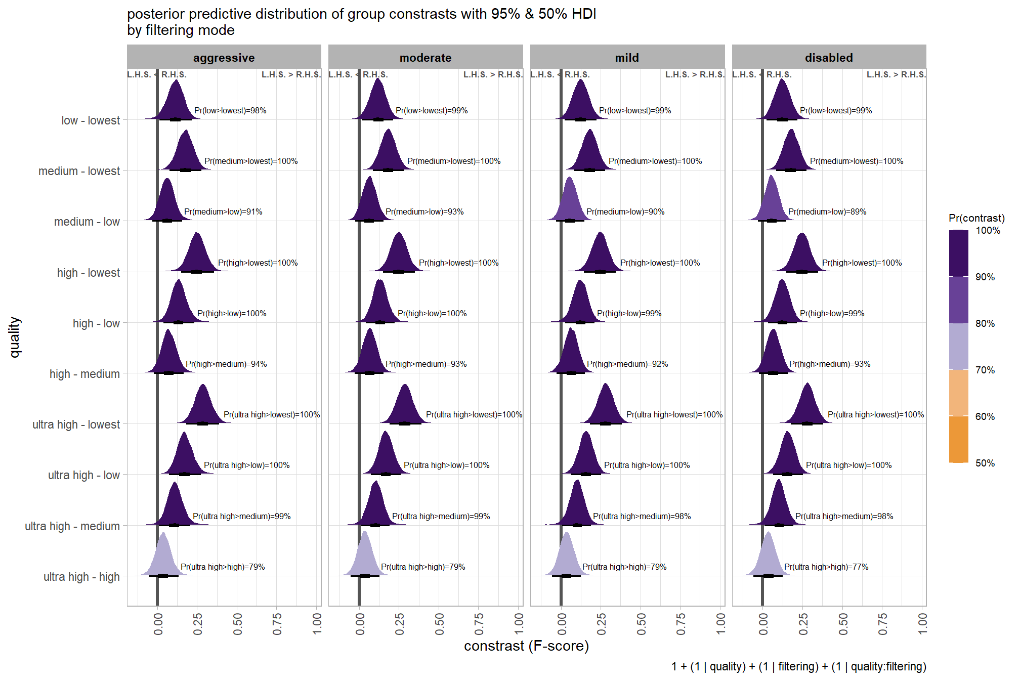
and summarize these contrasts
brms_contrast_temp %>%
  dplyr::group_by(contrast, depth_maps_generation_filtering_mode) %>%
  tidybayes::median_hdi(value) %>%
  dplyr::arrange(contrast, depth_maps_generation_filtering_mode) %>%
  dplyr::select(contrast, depth_maps_generation_filtering_mode, value, .lower, .upper) %>%

kableExtra::kbl(
    digits = 2
    , caption = "brms::brm model: 95% HDI of the posterior predictive distribution of group constrasts"
    , col.names = c(
      "quality contrast"
      , "filtering mode"
      , "difference (F-score)"
      , "HDI low", "HDI high"
    )
  ) %>%
  kableExtra::kable_styling() %>%
kableExtra::scroll_box(height = "6in")| quality contrast | filtering mode | difference (F-score) | HDI low | HDI high |
|---|---|---|---|---|
| ultra high - high | aggressive | 0.04 | -0.06 | 0.14 |
| ultra high - high | moderate | 0.04 | -0.05 | 0.13 |
| ultra high - high | mild | 0.04 | -0.06 | 0.13 |
| ultra high - high | disabled | 0.03 | -0.06 | 0.12 |
| ultra high - medium | aggressive | 0.11 | 0.01 | 0.21 |
| ultra high - medium | moderate | 0.10 | 0.01 | 0.19 |
| ultra high - medium | mild | 0.10 | 0.01 | 0.19 |
| ultra high - medium | disabled | 0.10 | 0.01 | 0.19 |
| ultra high - low | aggressive | 0.17 | 0.07 | 0.27 |
| ultra high - low | moderate | 0.17 | 0.07 | 0.26 |
| ultra high - low | mild | 0.16 | 0.07 | 0.25 |
| ultra high - low | disabled | 0.16 | 0.06 | 0.25 |
| ultra high - lowest | aggressive | 0.29 | 0.18 | 0.39 |
| ultra high - lowest | moderate | 0.29 | 0.19 | 0.39 |
| ultra high - lowest | mild | 0.28 | 0.18 | 0.38 |
| ultra high - lowest | disabled | 0.28 | 0.18 | 0.38 |
| high - medium | aggressive | 0.07 | -0.02 | 0.17 |
| high - medium | moderate | 0.07 | -0.03 | 0.15 |
| high - medium | mild | 0.06 | -0.03 | 0.15 |
| high - medium | disabled | 0.07 | -0.02 | 0.16 |
| high - low | aggressive | 0.13 | 0.04 | 0.23 |
| high - low | moderate | 0.13 | 0.04 | 0.22 |
| high - low | mild | 0.12 | 0.03 | 0.21 |
| high - low | disabled | 0.12 | 0.03 | 0.22 |
| high - lowest | aggressive | 0.25 | 0.15 | 0.36 |
| high - lowest | moderate | 0.25 | 0.15 | 0.35 |
| high - lowest | mild | 0.25 | 0.14 | 0.35 |
| high - lowest | disabled | 0.25 | 0.15 | 0.35 |
| medium - low | aggressive | 0.06 | -0.03 | 0.16 |
| medium - low | moderate | 0.07 | -0.03 | 0.15 |
| medium - low | mild | 0.06 | -0.03 | 0.15 |
| medium - low | disabled | 0.06 | -0.03 | 0.15 |
| medium - lowest | aggressive | 0.18 | 0.08 | 0.28 |
| medium - lowest | moderate | 0.18 | 0.09 | 0.28 |
| medium - lowest | mild | 0.18 | 0.08 | 0.28 |
| medium - lowest | disabled | 0.18 | 0.09 | 0.28 |
| low - lowest | aggressive | 0.12 | 0.01 | 0.22 |
| low - lowest | moderate | 0.12 | 0.02 | 0.21 |
| low - lowest | mild | 0.12 | 0.02 | 0.22 |
| low - lowest | disabled | 0.12 | 0.02 | 0.22 |
Kruschke (2015) notes that for the multiple nominal predictors model:
In applications with multiple levels of the factors, it is virtually always the case that we are interested in comparing particular levels with each other…These sorts of comparisons, which involve levels of a single factor and collapse across the other factor(s), are called main effect comparisons or contrasts.(p. 595)
First, let’s collapse across the filtering mode to compare the dense cloud quality setting effect.
In a hierarchical model structure, we have to make use of the re_formula argument within tidybayes::add_epred_draws
ptcld_validation_data %>%
  dplyr::distinct(depth_maps_generation_quality) %>%
  tidybayes::add_epred_draws(
    brms_f_mod2
    # this part is crucial
    , re_formula = ~ (1 | depth_maps_generation_quality)
  ) %>%
  dplyr::rename(value = .epred) %>%
  # plot
  ggplot(
    mapping = aes(
      x = value, y = depth_maps_generation_quality
      , fill = depth_maps_generation_quality
    )
  ) +
    tidybayes::stat_halfeye(
      point_interval = median_hdi, .width = .95
      , interval_color = "gray66"
      , shape = 21, point_color = "gray66", point_fill = "black"
      , justification = -0.01
    ) +
    scale_fill_viridis_d(option = "inferno", drop = F) +
    scale_x_continuous(breaks = scales::extended_breaks(n=8)) +
    labs(
      y = "quality", x = "F-score"
      , subtitle = "posterior predictive distribution of F-score with 95% HDI"
      , caption = form_temp
    ) +
    theme_light() +
    theme(legend.position = "none")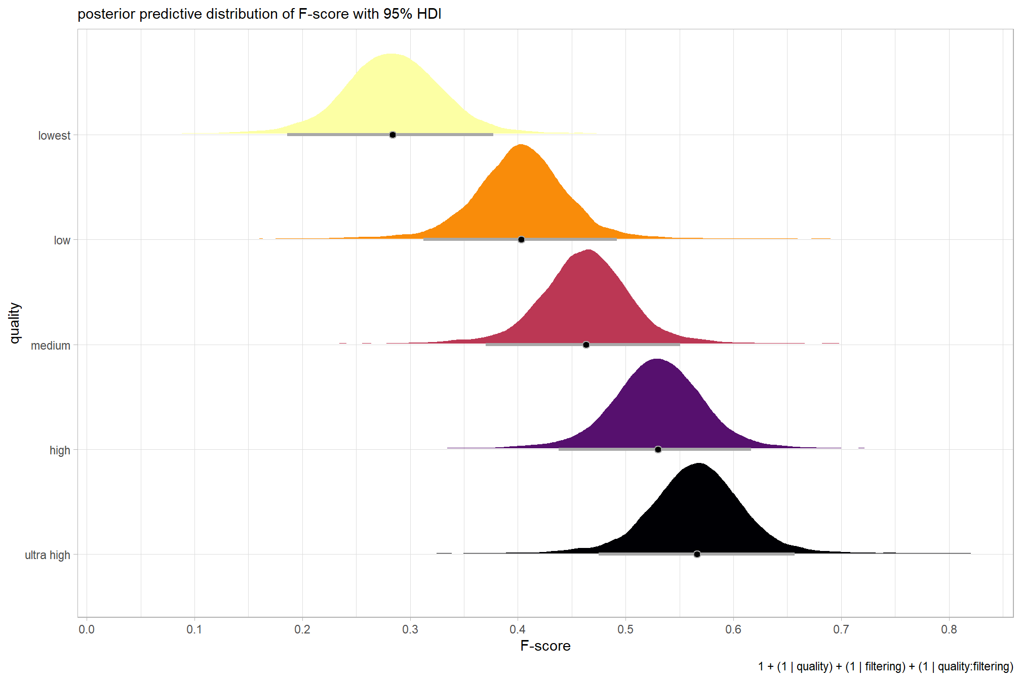
let’s compare these results to the results from our one nominal predictor model above
# let's compare these results to the results from our [one nominal predictor model above](#one_pred_mod)
ptcld_validation_data %>%
  dplyr::distinct(depth_maps_generation_quality) %>%
  tidybayes::add_epred_draws(
    brms_f_mod2
    # this part is crucial
    , re_formula = ~ (1 | depth_maps_generation_quality)
  ) %>%
  dplyr::mutate(value = .epred, src = "brms_f_mod2") %>%
  dplyr::bind_rows(
    ptcld_validation_data %>%
      dplyr::distinct(depth_maps_generation_quality) %>%
      tidybayes::add_epred_draws(brms_f_mod1) %>%
      dplyr::mutate(value = .epred, src = "brms_f_mod1")
  ) %>%
  ggplot(mapping = aes(y = src, x = value, color = src, group = src)) +
  tidybayes::stat_pointinterval(position = "dodge") +
  facet_grid(rows = vars(depth_maps_generation_quality), switch = "y") +
  scale_y_discrete(NULL, breaks = NULL) +
  scale_color_manual(values = viridis::turbo(n = 6, begin = 0.2, end = 0.8)[1:2]) +
  labs(
    y = "", x = "F-score"
    , color = "model"
  ) +
  theme_light() +
  theme(legend.position = "top", strip.text = element_text(color = "black", face = "bold"))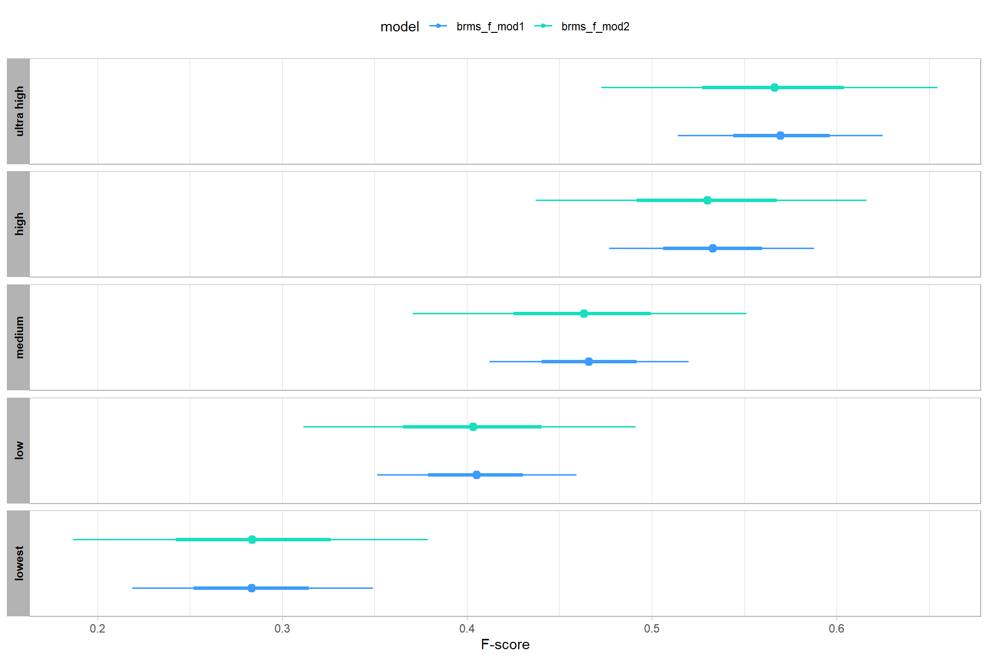
these results are as expected, with Kruschke (2015) noting:
It is important to realize that the estimates of interaction contrasts are typically much more uncertain than the estimates of simple effects or main effects…This large uncertainty of an interaction contrast is caused by the fact that it involves at least four sources of uncertainty (i.e., at least four groups of data), unlike its component simple effects which each involve only half of those sources of uncertainty. In general, interaction contrasts require a lot of data to estimate accurately. (p. 598)
For completeness, let’s also collapse across the dense cloud quality to compare the filtering mode setting effect.
In a hierarchical model structure, we have to make use of the re_formula argument within tidybayes::add_epred_draws
ptcld_validation_data %>%
  dplyr::distinct(depth_maps_generation_filtering_mode) %>%
  tidybayes::add_epred_draws(
    brms_f_mod2
    # this part is crucial
    , re_formula = ~ (1 | depth_maps_generation_filtering_mode)
  ) %>%
  dplyr::rename(value = .epred) %>%
  # plot
  ggplot(
    mapping = aes(
      x = value, y = depth_maps_generation_filtering_mode
      , fill = depth_maps_generation_filtering_mode
    )
  ) +
    tidybayes::stat_halfeye(
      point_interval = median_hdi, .width = .95
      , interval_color = "gray66"
      , shape = 21, point_color = "gray66", point_fill = "black"
      , justification = -0.01
    ) +
    scale_fill_viridis_d(option = "plasma", drop = F) +
    scale_x_continuous(breaks = scales::extended_breaks(n=8)) +
    labs(
      y = "filtering mode", x = "F-score"
      , subtitle = "posterior predictive distribution of F-score with 95% HDI"
      , caption = form_temp
    ) +
    theme_light() +
    theme(legend.position = "none")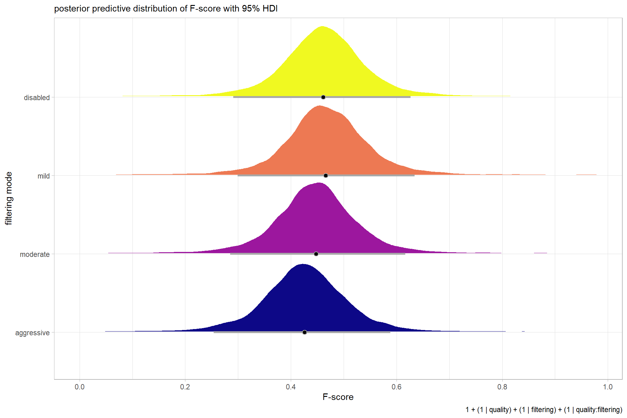
…it looks like the variation in F-score is driven by the dense cloud quality setting. We can quantify the variation in F-score by comparing the \(\sigma\) posteriors.
# extract the posterior draws
brms::as_draws_df(brms_f_mod2) %>%
  dplyr::select(c(sigma,tidyselect::starts_with("sd_"))) %>%
  tidyr::pivot_longer(dplyr::everything()) %>%
  # dplyr::group_by(name) %>%
  # tidybayes::median_hdi(value) %>%
  dplyr::mutate(
    name = name %>%
      stringr::str_replace_all("depth_maps_generation_quality", "quality") %>%
      stringr::str_replace_all("depth_maps_generation_filtering_mode", "filtering") %>%
      forcats::fct_reorder(value)
  ) %>%
# plot
  ggplot(aes(x = value, y = name)) +
  tidybayes::stat_dotsinterval(
    point_interval = median_hdi, .width = .95
    , justification = -0.04
    , shape = 21 #, point_size = 3
    , quantiles = 100
  ) +
  labs(x = "", y = "", caption = form_temp) +
  theme_light()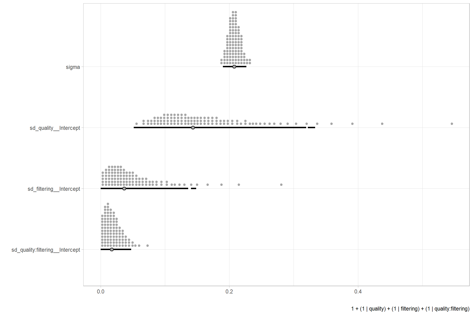
Finally we can perform model selection via information criteria, from section 10 in Kurz’s ebook supplement:
expected log predictive density (
elpd_loo), the estimated effective number of parameters (p_loo), and the Pareto smoothed importance-sampling leave-one-out cross-validation (PSIS-LOO;looic). Each estimate comes with a standard error (i.e.,SE). Like other information criteria, the LOO values aren’t of interest in and of themselves. However, the estimate of one model’s LOO relative to that of another can be of great interest. We generally prefer models with lower information criteria. With thebrms::loo_compare()function, we can compute a formal difference score between two models…Thebrms::loo_compare()output rank orders the models such that the best fitting model appears on top.
brms_f_mod1 = brms::add_criterion(brms_f_mod1, criterion = c("loo", "waic"))
brms_f_mod2 = brms::add_criterion(brms_f_mod2, criterion = c("loo", "waic"))
brms::loo_compare(brms_f_mod1, brms_f_mod2, criterion = "loo")
## elpd_diff se_diff
## brms_f_mod1 0.0 0.0
## brms_f_mod2 -1.7 1.2These models are not significantly different suggesting that the filtering mode is not contributing much to the variation in SfM-derived tree detection reliability after accounting for the quality setting
6.5 Three Nominal Predictors
Now, we’ll add the SfM processing software to our model which includes the depth map generation quality and the depth map filtering parameters to quantify the SfM-derived tree detection performance based on the F-score.
6.5.1 Summary Statistics
Summary statistics by group:
ptcld_validation_data %>%
  dplyr::group_by(depth_maps_generation_quality, depth_maps_generation_filtering_mode, software) %>%
  dplyr::summarise(
    mean_f_score = mean(f_score, na.rm = T)
    # , med_f_score = median(f_score, na.rm = T)
    , sd_f_score = sd(f_score, na.rm = T)
    , n = dplyr::n()
  ) %>%
  kableExtra::kbl(
    digits = 2
    , caption = "summary statistics: F-score by dense cloud quality, filtering mode, and software"
    , col.names = c(
      "quality"
      , "filtering mode"
      , "software"
      , "mean F-score"
      , "sd"
      , "n"
    )
  ) %>%
  kableExtra::kable_styling() %>%
kableExtra::scroll_box(height = "8in")| quality | filtering mode | software | mean F-score | sd | n |
|---|---|---|---|---|---|
| ultra high | aggressive | METASHAPE | 0.56 | 0.21 | 5 |
| ultra high | aggressive | OPENDRONEMAP | 0.60 | 0.21 | 5 |
| ultra high | moderate | METASHAPE | 0.61 | 0.23 | 5 |
| ultra high | moderate | OPENDRONEMAP | 0.58 | 0.20 | 5 |
| ultra high | moderate | PIX4D | 0.55 | 0.24 | 5 |
| ultra high | mild | METASHAPE | 0.62 | 0.23 | 5 |
| ultra high | mild | OPENDRONEMAP | 0.58 | 0.19 | 5 |
| ultra high | mild | PIX4D | 0.54 | 0.24 | 5 |
| ultra high | disabled | METASHAPE | 0.61 | 0.24 | 5 |
| ultra high | disabled | OPENDRONEMAP | 0.54 | 0.23 | 5 |
| ultra high | disabled | PIX4D | 0.54 | 0.25 | 5 |
| high | aggressive | METASHAPE | 0.51 | 0.19 | 5 |
| high | aggressive | OPENDRONEMAP | 0.53 | 0.17 | 5 |
| high | moderate | METASHAPE | 0.60 | 0.24 | 5 |
| high | moderate | OPENDRONEMAP | 0.47 | 0.21 | 5 |
| high | moderate | PIX4D | 0.54 | 0.24 | 5 |
| high | mild | METASHAPE | 0.61 | 0.24 | 5 |
| high | mild | OPENDRONEMAP | 0.48 | 0.21 | 5 |
| high | mild | PIX4D | 0.53 | 0.24 | 5 |
| high | disabled | METASHAPE | 0.61 | 0.24 | 5 |
| high | disabled | OPENDRONEMAP | 0.47 | 0.22 | 5 |
| high | disabled | PIX4D | 0.55 | 0.25 | 5 |
| medium | aggressive | METASHAPE | 0.41 | 0.18 | 5 |
| medium | aggressive | OPENDRONEMAP | 0.36 | 0.15 | 5 |
| medium | moderate | METASHAPE | 0.54 | 0.20 | 5 |
| medium | moderate | OPENDRONEMAP | 0.34 | 0.20 | 5 |
| medium | moderate | PIX4D | 0.54 | 0.23 | 5 |
| medium | mild | METASHAPE | 0.60 | 0.25 | 5 |
| medium | mild | OPENDRONEMAP | 0.33 | 0.19 | 5 |
| medium | mild | PIX4D | 0.56 | 0.25 | 5 |
| medium | disabled | METASHAPE | 0.57 | 0.25 | 5 |
| medium | disabled | OPENDRONEMAP | 0.33 | 0.22 | 5 |
| medium | disabled | PIX4D | 0.55 | 0.24 | 5 |
| low | aggressive | METASHAPE | 0.25 | 0.12 | 5 |
| low | aggressive | OPENDRONEMAP | 0.34 | 0.13 | 5 |
| low | moderate | METASHAPE | 0.39 | 0.20 | 5 |
| low | moderate | OPENDRONEMAP | 0.34 | 0.20 | 5 |
| low | moderate | PIX4D | 0.38 | 0.17 | 5 |
| low | mild | METASHAPE | 0.49 | 0.21 | 5 |
| low | mild | OPENDRONEMAP | 0.34 | 0.21 | 5 |
| low | mild | PIX4D | 0.54 | 0.24 | 5 |
| low | disabled | METASHAPE | 0.48 | 0.24 | 5 |
| low | disabled | OPENDRONEMAP | 0.33 | 0.22 | 5 |
| low | disabled | PIX4D | 0.54 | 0.24 | 5 |
| lowest | aggressive | METASHAPE | 0.11 | 0.10 | 5 |
| lowest | aggressive | OPENDRONEMAP | 0.36 | 0.16 | 5 |
| lowest | moderate | METASHAPE | 0.15 | 0.10 | 5 |
| lowest | moderate | OPENDRONEMAP | 0.36 | 0.22 | 5 |
| lowest | mild | METASHAPE | 0.27 | 0.19 | 5 |
| lowest | mild | OPENDRONEMAP | 0.32 | 0.19 | 5 |
| lowest | disabled | METASHAPE | 0.27 | 0.22 | 5 |
| lowest | disabled | OPENDRONEMAP | 0.33 | 0.22 | 5 |
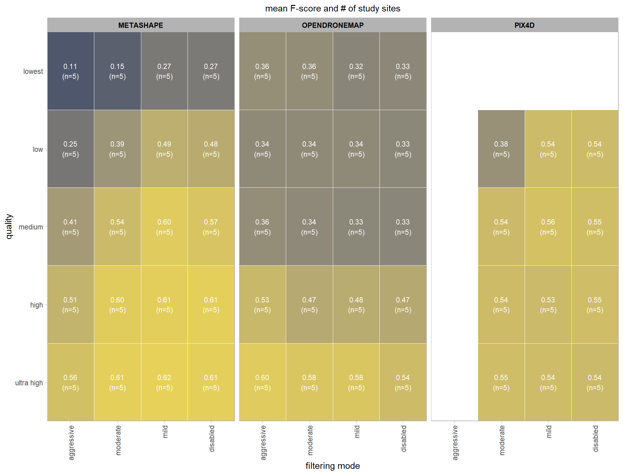
we can view this data by using ggplot2::geom_tile
ptcld_validation_data %>%
  dplyr::group_by(software, depth_maps_generation_quality, depth_maps_generation_filtering_mode) %>%
  # collapse across study site
  dplyr::summarise(
    mean_f_score = mean(f_score, na.rm = T)
    # , med_f_score = median(f_score, na.rm = T)
    , sd_f_score = sd(f_score, na.rm = T)
    , n = dplyr::n()
  ) %>%
  ggplot(mapping = aes(
    y = depth_maps_generation_quality
    , x = depth_maps_generation_filtering_mode
    , fill = mean_f_score
    , label = paste0(scales::comma(mean_f_score,accuracy = 0.01), "\n(n=", n,")")
  )) +
  geom_tile(color = "white") +
  geom_text(color = "white", size = 3) +
  facet_grid(cols = vars(software)) +
  scale_x_discrete(expand = c(0, 0)) +
  scale_y_discrete(expand = c(0, 0)) +
  scale_fill_viridis_c(option = "cividis", begin = 0.3, end = 0.9) +
  labs(
    x = "filtering mode"
    , y = "quality"
    , fill = "F-score"
    , subtitle = "mean F-score and # of study sites"
  ) +
  theme_light() +
  theme(
    legend.position = "none"
    , axis.text.x = element_text(angle = 90, vjust = 0.5, hjust = 1)
    , panel.background = element_blank()
    , panel.grid = element_blank()
    , plot.subtitle = element_text(hjust = 0.5)
    , strip.text = element_text(color = "black", face = "bold")
  )
6.5.2 Bayesian
Kruschke (2015) describes the Hierarchical Bayesian approach to extend our two nominal predictor model to include another nominal predictor (referred to as “subject” here but the methodology applies for other nominal variables):
When every subject contributes many measurements to every cell, then the model of the situation is a straight-forward extension of the models we have already considered. We merely add “subject” as another nominal predictor in the model, with each individual subject being a level of the predictor. If there is one predictor other than subject, the model becomes
\[ y = \beta_0 + \overrightarrow \beta_1 \overrightarrow x_1 + \overrightarrow \beta_S \overrightarrow x_S + \overrightarrow \beta_{1 \times S} \overrightarrow x_{1 \times S} \]
This is exactly the two-predictor model we have already considered, with the second predictor being subject. When there are two predictors other than subject, the model becomes
\[\begin{align*} y = & \; \beta_0 & \text{baseline} \\ & + \overrightarrow \beta_1 \overrightarrow x_1 + \overrightarrow \beta_2 \overrightarrow x_2 + \overrightarrow \beta_S \overrightarrow x_S & \text{main effects} \\ & + \overrightarrow \beta_{1 \times 2} \overrightarrow x_{1 \times 2} + \overrightarrow \beta_{1 \times S} \overrightarrow x_{1 \times S} + \overrightarrow \beta_{2 \times S} \overrightarrow x_{2 \times S} & \text{two-way interactions} \\ & + \overrightarrow \beta_{1 \times 2 \times S} \overrightarrow x_{1 \times 2 \times S} & \text{three-way interactions} \end{align*}\]
This model includes all the two-way interactions of the factors, plus the three-way interaction. (p. 607)
The metric predicted variable with three nominal predictor variables model has the form:
\[\begin{align*} y_{i} \sim & \operatorname{Normal} \bigl(\mu_{i}, \sigma_{y} \bigr) \\ \mu_{i} = & \beta_0 \\ & + \sum_{j} \beta_{1[j]} x_{1[j]} + \sum_{k} \beta_{2[k]} x_{2[k]} + \sum_{f} \beta_{3[f]} x_{3[f]} \\ & + \sum_{j,k} \beta_{1\times2[j,k]} x_{1\times2[j,k]} + \sum_{j,f} \beta_{1\times3[j,f]} x_{1\times3[j,f]} + \sum_{k,f} \beta_{2\times3[k,f]} x_{2\times3[k,f]} \\ & + \sum_{j,k,f} \beta_{1\times2\times3[j,k,f]} x_{1\times2\times3[j,k,f]} \\ \beta_{0} \sim & \operatorname{Normal}(0,100) \\ \beta_{1[j]} \sim & \operatorname{Normal}(0,\sigma_{\beta_{1}}) \\ \beta_{2[k]} \sim & \operatorname{Normal}(0,\sigma_{\beta_{2}}) \\ \beta_{3[f]} \sim & \operatorname{Normal}(0,\sigma_{\beta_{3}}) \\ \beta_{1\times2[j,k]} \sim & \operatorname{Normal}(0,\sigma_{\beta_{1\times2}}) \\ \beta_{1\times3[j,f]} \sim & \operatorname{Normal}(0,\sigma_{\beta_{1\times3}}) \\ \beta_{2\times3[k,f]} \sim & \operatorname{Normal}(0,\sigma_{\beta_{2\times3}}) \\ \sigma_{\beta_{1}} \sim & \operatorname{Gamma}(1.28,0.005) \\ \sigma_{\beta_{2}} \sim & \operatorname{Gamma}(1.28,0.005) \\ \sigma_{\beta_{3}} \sim & \operatorname{Gamma}(1.28,0.005) \\ \sigma_{\beta_{1\times2}} \sim & \operatorname{Gamma}(1.28,0.005) \\ \sigma_{\beta_{1\times3}} \sim & \operatorname{Gamma}(1.28,0.005) \\ \sigma_{\beta_{2\times3}} \sim & \operatorname{Gamma}(1.28,0.005) \\ \sigma_{y} \sim & {\sf Cauchy} (0,109) \\ \end{align*}\]
, where \(j\) is the depth map generation quality setting corresponding to observation \(i\), \(k\) is the depth map filtering mode setting corresponding to observation \(i\), and \(f\) is the processing software corresponding to observation \(i\)
for this model, we’ll define the priors following Kurz who notes that:
The noise standard deviation \(\sigma_y\) is depicted in the prior statement including the argument
class = sigma…in order to be weakly informative, we will use the half-Cauchy. Recall that since the brms default is to set the lower bound for any variance parameter to 0, there’s no need to worry about doing so ourselves. So even though the syntax only indicatescauchy, it’s understood to mean Cauchy with a lower bound at zero; since the mean is usually 0, that makes this a half-Cauchy…The tails of the half-Cauchy are sufficiently fat that, in practice, I’ve found it doesn’t matter much what you set the \(SD\) of its prior to.
# from Kurz:
gamma_a_b_from_omega_sigma = function(mode, sd) {
  if (mode <= 0) stop("mode must be > 0")
  if (sd   <= 0) stop("sd must be > 0")
  rate = (mode + sqrt(mode^2 + 4 * sd^2)) / (2 * sd^2)
  shape = 1 + mode * rate
  return(list(shape = shape, rate = rate))
}

mean_y_temp = mean(ptcld_validation_data$f_score)
sd_y_temp   = sd(ptcld_validation_data$f_score)

omega_temp = sd_y_temp / 2
sigma_temp = 2 * sd_y_temp

s_r_temp = gamma_a_b_from_omega_sigma(mode = omega_temp, sd = sigma_temp)

stanvars_temp =
  brms::stanvar(mean_y_temp,    name = "mean_y") +
  brms::stanvar(sd_y_temp,      name = "sd_y") +
  brms::stanvar(s_r_temp$shape, name = "alpha") +
  brms::stanvar(s_r_temp$rate,  name = "beta")
Now fit the model.
brms_f_mod3 = brms::brm(
formula = f_score ~
# baseline
1 +
# main effects
(1 | depth_maps_generation_quality) +
(1 | depth_maps_generation_filtering_mode) +
(1 | software) +
# two-way interactions
(1 | depth_maps_generation_quality:depth_maps_generation_filtering_mode) +
(1 | depth_maps_generation_quality:software) +
(1 | depth_maps_generation_filtering_mode:software) +
# three-way interactions
(1 | depth_maps_generation_quality:depth_maps_generation_filtering_mode:software)
, data = ptcld_validation_data
, family = brms::brmsfamily(family = "gaussian")
, iter = 20000, warmup = 10000, chains = 4
, control = list(adapt_delta = 0.999, max_treedepth = 13)
, cores = round(parallel::detectCores()/2)
, prior = c(
brms::prior(normal(mean_y, sd_y * 5), class = "Intercept")
, brms::prior(gamma(alpha, beta), class = "sd")
, brms::prior(cauchy(0, sd_y), class = "sigma")
)
, stanvars = stanvars_temp
, file = paste0(rootdir, "/fits/brms_f_mod3")
)
# https://mc-stan.org/misc/warnings.html#divergent-transitions-after-warmup
# https://mc-stan.org/misc/warnings.html#bulk-ess
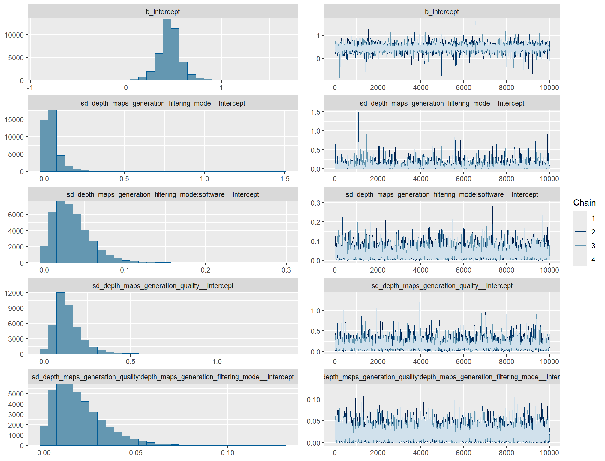
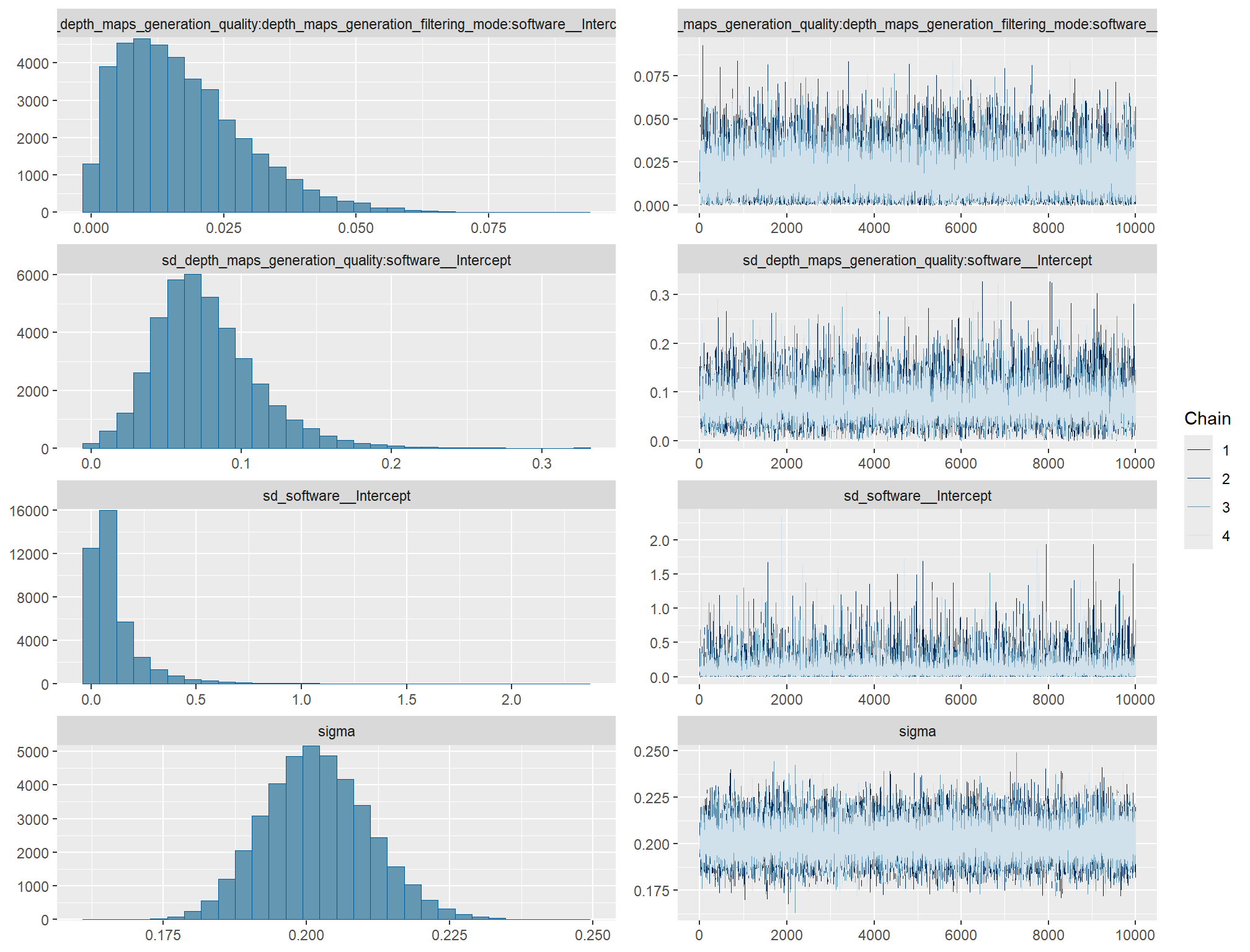
# https://mc-stan.org/misc/warnings.html#tail-ess check the trace plots for problems with convergence of the Markov chains
check the prior distributions
# check priors
brms::prior_summary(brms_f_mod3) %>%
  kableExtra::kbl() %>%
kableExtra::kable_styling()| prior | class | coef | group | resp | dpar | nlpar | lb | ub | source |
|---|---|---|---|---|---|---|---|---|---|
| normal(mean_y, sd_y * 5) | Intercept | user | |||||||
| gamma(alpha, beta) | sd | 0 | user | ||||||
| sd | depth_maps_generation_filtering_mode | default | |||||||
| sd | Intercept | depth_maps_generation_filtering_mode | default | ||||||
| sd | depth_maps_generation_filtering_mode:software | default | |||||||
| sd | Intercept | depth_maps_generation_filtering_mode:software | default | ||||||
| sd | depth_maps_generation_quality | default | |||||||
| sd | Intercept | depth_maps_generation_quality | default | ||||||
| sd | depth_maps_generation_quality:depth_maps_generation_filtering_mode | default | |||||||
| sd | Intercept | depth_maps_generation_quality:depth_maps_generation_filtering_mode | default | ||||||
| sd | depth_maps_generation_quality:depth_maps_generation_filtering_mode:software | default | |||||||
| sd | Intercept | depth_maps_generation_quality:depth_maps_generation_filtering_mode:software | default | ||||||
| sd | depth_maps_generation_quality:software | default | |||||||
| sd | Intercept | depth_maps_generation_quality:software | default | ||||||
| sd | software | default | |||||||
| sd | Intercept | software | default | ||||||
| cauchy(0, sd_y) | sigma | 0 | user |
The brms::brm model summary
We won’t clutter the output here but this can be run if you are following along on your own
brms_f_mod3 %>%
  brms::posterior_summary() %>%
  as.data.frame() %>%
  tibble::rownames_to_column(var = "parameter") %>%
  dplyr::rename_with(tolower) %>%
  dplyr::filter(
    stringr::str_starts(parameter, "b_")
    | stringr::str_starts(parameter, "r_")
    | stringr::str_starts(parameter, "sd_")
    | parameter == "sigma"
  ) %>%
  dplyr::mutate(
    parameter = parameter %>%
      stringr::str_replace_all("depth_maps_generation_quality", "quality") %>%
      stringr::str_replace_all("depth_maps_generation_filtering_mode", "filtering")
  ) %>%
  kableExtra::kbl(digits = 2, caption = "Bayesian 3 nominal predictors for F-score") %>%
  kableExtra::kable_styling() %>%
  kableExtra::scroll_box(height = "8in")
We can look at the model noise standard deviation \(\sigma_y\)
# get formula
form_temp = brms_f_mod3$formula$formula[3] %>%
  as.character() %>% get_frmla_text() %>%
  stringr::str_replace_all("depth_maps_generation_quality", "quality") %>%
  stringr::str_replace_all("depth_maps_generation_filtering_mode", "filtering")
# extract the posterior draws
brms::as_draws_df(brms_f_mod3) %>%
# plot
  ggplot(aes(x = sigma, y = 0)) +
  tidybayes::stat_dotsinterval(
    point_interval = median_hdi, .width = .95
    , justification = -0.04
    , shape = 21, point_size = 3
    , quantiles = 100
  ) +
  scale_y_continuous(NULL, breaks = NULL) +
  labs(
    x = latex2exp::TeX("$\\sigma_y$")
    , caption = form_temp
  ) +
  theme_light()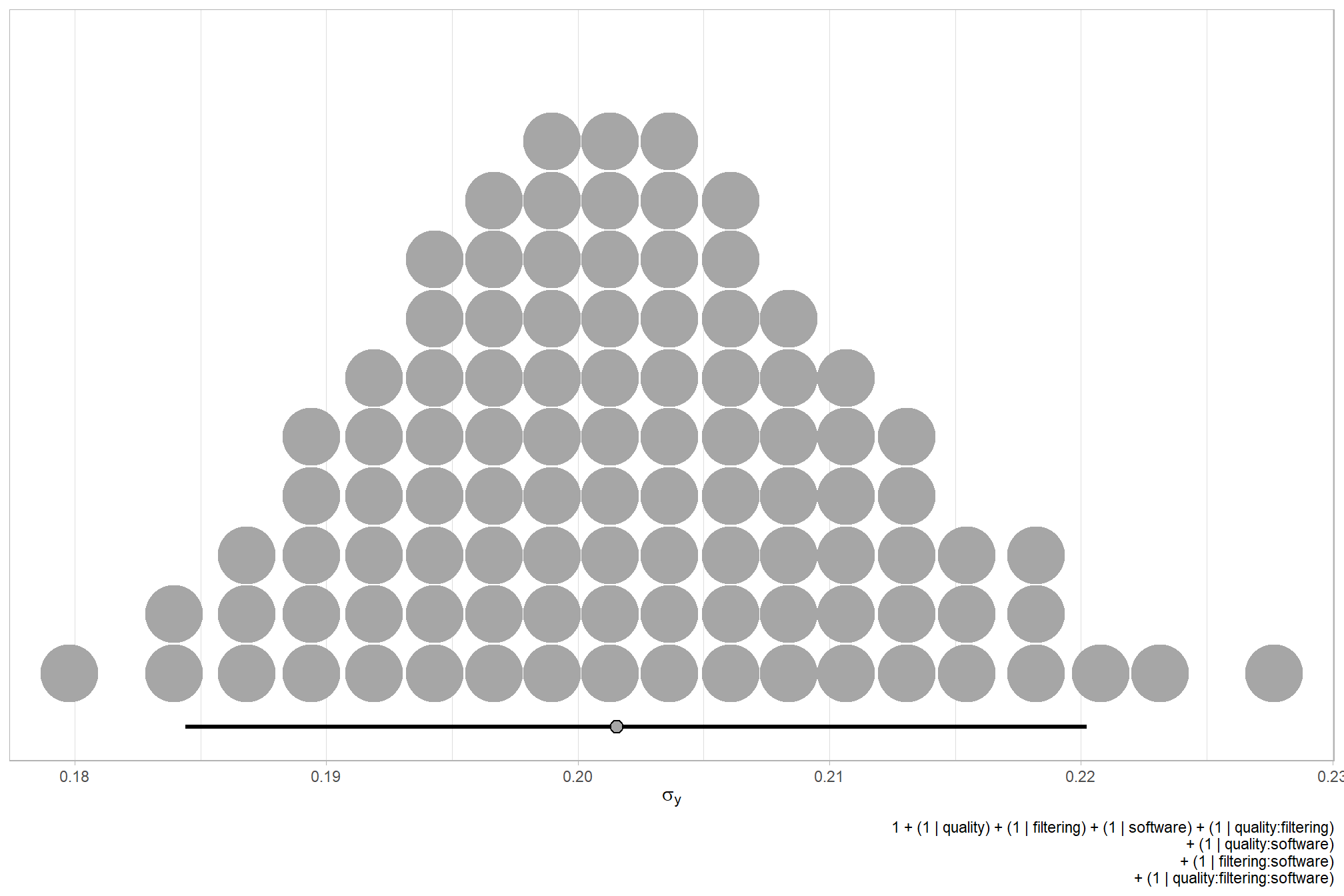
how is it compared to our other models?
# how is it compared to our other models?
dplyr::bind_rows(
    brms::as_draws_df(brms_f_mod1) %>% tidybayes::median_hdi(sigma) %>% dplyr::mutate(model = "one nominal predictor")
    , brms::as_draws_df(brms_f_mod2) %>% tidybayes::median_hdi(sigma) %>% dplyr::mutate(model = "two nominal predictor")
    , brms::as_draws_df(brms_f_mod3) %>% tidybayes::median_hdi(sigma) %>% dplyr::mutate(model = "three nominal predictor")
  ) %>%
  dplyr::relocate(model) %>%
  kableExtra::kbl(digits = 2, caption = "brms::brm model noise standard deviation comparison") %>%
kableExtra::kable_styling()| model | sigma | .lower | .upper | .width | .point | .interval |
|---|---|---|---|---|---|---|
| one nominal predictor | 0.21 | 0.19 | 0.23 | 0.95 | median | hdi |
| two nominal predictor | 0.21 | 0.19 | 0.23 | 0.95 | median | hdi |
| three nominal predictor | 0.20 | 0.18 | 0.22 | 0.95 | median | hdi |
plot the posterior predictive distributions of the conditional means with the median F-score and the 95% highest posterior density interval (HDI)
Note that how within tidybayes::add_epred_draws, we used the re_formula argument to average over the random effects of software. For this model we have to collapse across the software effects to compare the dense cloud quality and filtering mode setting effects.
ptcld_validation_data %>%
  dplyr::distinct(depth_maps_generation_quality, depth_maps_generation_filtering_mode) %>%
  tidybayes::add_epred_draws(
    brms_f_mod3, allow_new_levels = T
    # this part is crucial
    , re_formula = ~ (1 | depth_maps_generation_quality) +
      (1 | depth_maps_generation_filtering_mode) +
      (1 | depth_maps_generation_quality:depth_maps_generation_filtering_mode)
  ) %>%
  dplyr::rename(value = .epred) %>%
  dplyr::mutate(depth_maps_generation_quality = depth_maps_generation_quality %>% forcats::fct_rev()) %>%
  # plot
  ggplot(
    mapping = aes(
      y = value, x = depth_maps_generation_filtering_mode
      , fill = depth_maps_generation_filtering_mode
    )
  ) +
    tidybayes::stat_eye(
      point_interval = median_hdi, .width = .95
      , slab_alpha = 0.8
      , interval_color = "black", linewidth = 1
      , point_color = "black", point_fill = "black", point_size = 1
    ) +
    scale_fill_viridis_d(option = "plasma", drop = F) +
    scale_y_continuous(breaks = scales::extended_breaks(n=10)) +
    facet_grid(cols = vars(depth_maps_generation_quality)) +
    labs(
      x = "filtering mode", y = "F-score"
      , subtitle = "posterior predictive distribution of F-score with 95% HDI\nby dense cloud quality"
      , fill = "Filtering Mode"
      , caption = form_temp
    ) +
    theme_light() +
    theme(
      legend.position = "none"
      , legend.direction  = "horizontal"
      , axis.text.x = element_text(angle = 90, vjust = 0.5, hjust = 1)
      , strip.text = element_text(color = "black", face = "bold")
) 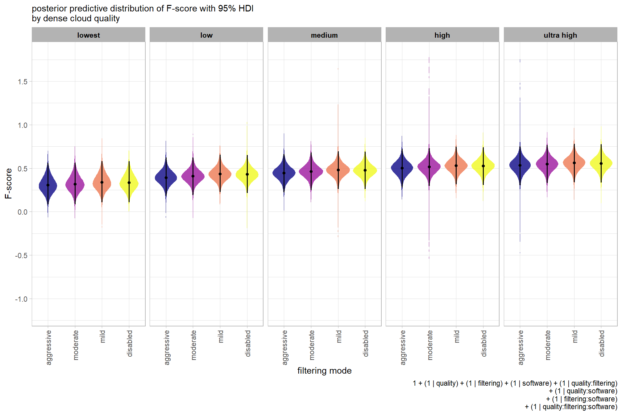
we can also make pairwise comparisons so long as we continue using tidybayes::add_epred_draws with the re_formula argument
brms_contrast_temp =
  ptcld_validation_data %>%
    dplyr::distinct(depth_maps_generation_quality, depth_maps_generation_filtering_mode) %>%
    tidybayes::add_epred_draws(
      brms_f_mod3, allow_new_levels = T
      # this part is crucial
      , re_formula = ~ (1 | depth_maps_generation_quality) +
        (1 | depth_maps_generation_filtering_mode) +
        (1 | depth_maps_generation_quality:depth_maps_generation_filtering_mode)
    ) %>%
    dplyr::rename(value = .epred) %>%
    tidybayes::compare_levels(
      value
      , by = depth_maps_generation_quality
      , comparison =
        contrast_list
        # tidybayes::emmeans_comparison("revpairwise")
        #"pairwise"
    ) %>%
    dplyr::rename(contrast = depth_maps_generation_quality)

# separate contrast
brms_contrast_temp = brms_contrast_temp %>%
  dplyr::ungroup() %>%
  tidyr::separate_wider_delim(
    cols = contrast
    , delim = " - "
    , names = paste0(
        "sorter"
        , 1:(max(stringr::str_count(brms_contrast_temp$contrast, "-"))+1)
      )
    , too_few = "align_start"
    , cols_remove = F
  ) %>%
  dplyr::filter(sorter1!=sorter2) %>%
  dplyr::mutate(
    dplyr::across(
      tidyselect::starts_with("sorter")
      , .fns = function(x){factor(
        x, ordered = T
        , levels = levels(ptcld_validation_data$depth_maps_generation_quality)
      )}
    )
    , contrast = contrast %>%
      forcats::fct_reorder(
        paste0(as.numeric(sorter1), as.numeric(sorter2)) %>%
        as.numeric()
      )
    , depth_maps_generation_filtering_mode = depth_maps_generation_filtering_mode %>%
      factor(
        levels = levels(ptcld_validation_data$depth_maps_generation_filtering_mode)
        , ordered = T
      )
  ) %>%
  # median_hdi summary for coloring
  dplyr::group_by(contrast, depth_maps_generation_filtering_mode) %>%
  make_contrast_vars()

# what?
brms_contrast_temp %>% dplyr::glimpse()
## Rows: 1,600,000
## Columns: 19
## Groups: contrast, depth_maps_generation_filtering_mode [40]
## $ depth_maps_generation_filtering_mode <ord> aggressive, aggressive, aggressiv…
## $ .chain <int> NA, NA, NA, NA, NA, NA, NA, NA, N…
## $ .iteration <int> NA, NA, NA, NA, NA, NA, NA, NA, N…
## $ .draw <int> 1, 2, 3, 4, 5, 6, 7, 8, 9, 10, 11…
## $ sorter1 <ord> ultra high, ultra high, ultra hig…
## $ sorter2 <ord> high, high, high, high, high, hig…
## $ contrast <fct> ultra high - high, ultra high - h…
## $ value <dbl> -0.087610941, 0.085047329, -0.131…
## $ median_hdi_est <dbl> 0.03005148, 0.03005148, 0.0300514…
## $ median_hdi_lower <dbl> -0.1129854, -0.1129854, -0.112985…
## $ median_hdi_upper <dbl> 0.1723716, 0.1723716, 0.1723716, …
## $ pr_gt_zero <chr> "67%", "67%", "67%", "67%", "67%"…
## $ pr_lt_zero <chr> "33%", "33%", "33%", "33%", "33%"…
## $ is_diff_dir <lgl> FALSE, TRUE, FALSE, TRUE, TRUE, F…
## $ pr_diff <dbl> 0.674575, 0.674575, 0.674575, 0.6…
## $ pr_diff_lab <chr> "Pr(ultra high>high)=67%", "Pr(ul…
## $ pr_diff_lab_sm <chr> "Pr(>0)=67%", "Pr(>0)=67%", "Pr(>…
## $ pr_diff_lab_pos <dbl> 0.1852995, 0.1852995, 0.1852995, …
## $ sig_level <ord> <80%, <80%, <80%, <80%, <80%, <80…plot it
plt_contrast(
  brms_contrast_temp, caption_text = form_temp
  , y_axis_title = "quality"
  , facet = "depth_maps_generation_filtering_mode"
  , label_size = 2.1
  , x_expand = c(0,0.6)
) +
  labs(
    subtitle = "posterior predictive distribution of group constrasts with 95% & 50% HDI\nby filtering mode"
  )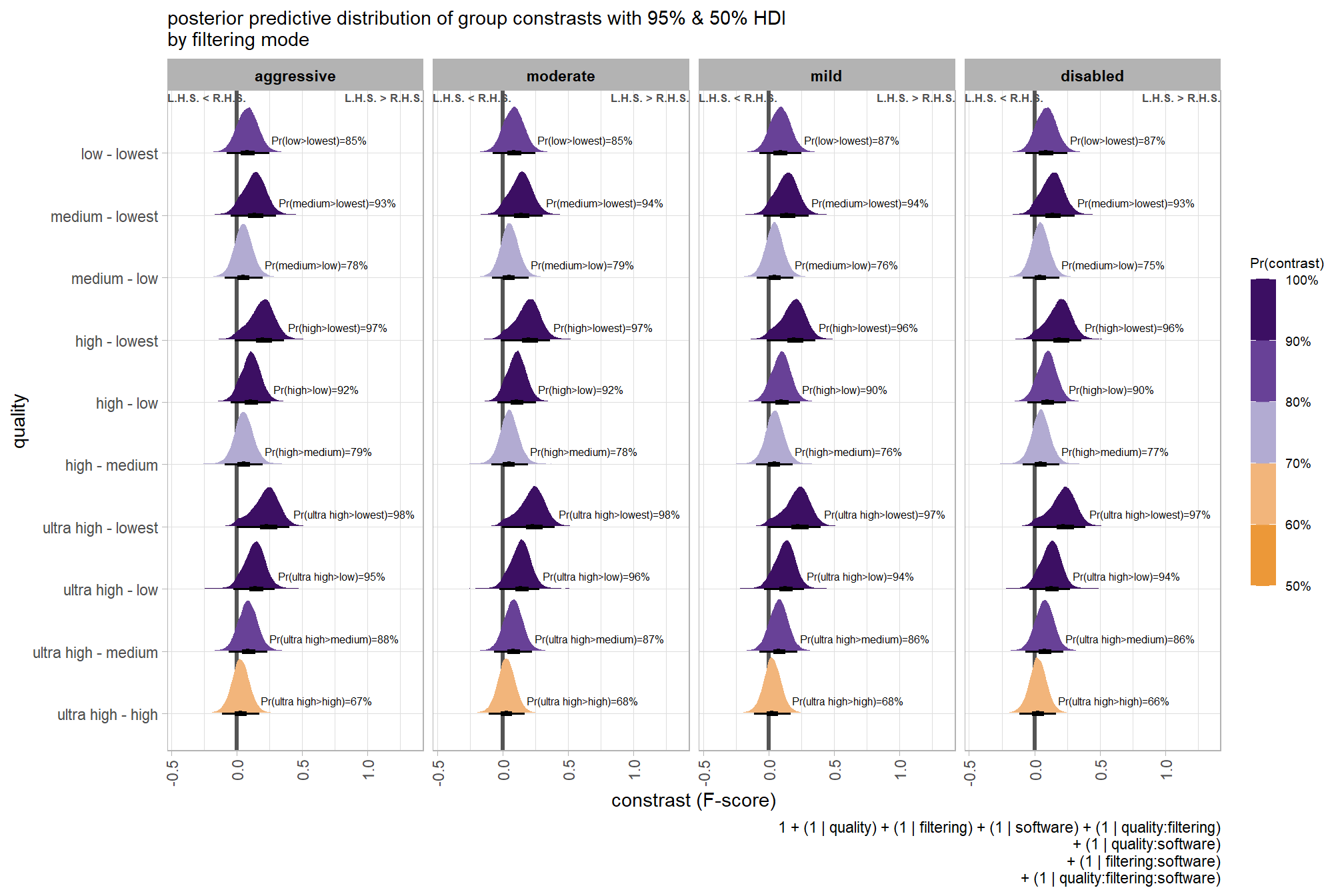
and summarize these contrasts
brms_contrast_temp %>%
  dplyr::group_by(contrast, depth_maps_generation_filtering_mode) %>%
  tidybayes::median_hdi(value) %>%
  dplyr::arrange(contrast, depth_maps_generation_filtering_mode) %>%
  dplyr::select(contrast, depth_maps_generation_filtering_mode, value, .lower, .upper) %>%

kableExtra::kbl(
    digits = 2
    , caption = "brms::brm model: 95% HDI of the posterior predictive distribution of group constrasts"
    , col.names = c(
      "quality contrast"
      , "filtering mode"
      , "difference (F-score)"
      , "HDI low", "HDI high"
    )
  ) %>%
  kableExtra::kable_styling() %>%
kableExtra::scroll_box(height = "6in")| quality contrast | filtering mode | difference (F-score) | HDI low | HDI high |
|---|---|---|---|---|
| ultra high - high | aggressive | 0.03 | -0.11 | 0.17 |
| ultra high - high | moderate | 0.03 | -0.11 | 0.17 |
| ultra high - high | mild | 0.03 | -0.11 | 0.17 |
| ultra high - high | disabled | 0.03 | -0.11 | 0.17 |
| ultra high - medium | aggressive | 0.09 | -0.06 | 0.23 |
| ultra high - medium | moderate | 0.08 | -0.06 | 0.23 |
| ultra high - medium | mild | 0.08 | -0.07 | 0.22 |
| ultra high - medium | disabled | 0.08 | -0.07 | 0.22 |
| ultra high - low | aggressive | 0.14 | -0.02 | 0.29 |
| ultra high - low | moderate | 0.14 | -0.02 | 0.28 |
| ultra high - low | mild | 0.13 | -0.03 | 0.27 |
| ultra high - low | disabled | 0.13 | -0.04 | 0.27 |
| ultra high - lowest | aggressive | 0.23 | 0.00 | 0.40 |
| ultra high - lowest | moderate | 0.23 | 0.00 | 0.40 |
| ultra high - lowest | mild | 0.23 | 0.00 | 0.40 |
| ultra high - lowest | disabled | 0.22 | -0.01 | 0.39 |
| high - medium | aggressive | 0.05 | -0.09 | 0.20 |
| high - medium | moderate | 0.05 | -0.09 | 0.20 |
| high - medium | mild | 0.05 | -0.10 | 0.19 |
| high - medium | disabled | 0.05 | -0.09 | 0.19 |
| high - low | aggressive | 0.11 | -0.04 | 0.26 |
| high - low | moderate | 0.11 | -0.04 | 0.25 |
| high - low | mild | 0.10 | -0.05 | 0.24 |
| high - low | disabled | 0.10 | -0.05 | 0.24 |
| high - lowest | aggressive | 0.20 | -0.01 | 0.36 |
| high - lowest | moderate | 0.20 | -0.01 | 0.36 |
| high - lowest | mild | 0.19 | -0.01 | 0.36 |
| high - lowest | disabled | 0.19 | -0.02 | 0.36 |
| medium - low | aggressive | 0.05 | -0.09 | 0.20 |
| medium - low | moderate | 0.05 | -0.08 | 0.20 |
| medium - low | mild | 0.05 | -0.09 | 0.19 |
| medium - low | disabled | 0.05 | -0.09 | 0.19 |
| medium - lowest | aggressive | 0.14 | -0.05 | 0.30 |
| medium - lowest | moderate | 0.14 | -0.04 | 0.31 |
| medium - lowest | mild | 0.14 | -0.04 | 0.31 |
| medium - lowest | disabled | 0.14 | -0.03 | 0.31 |
| low - lowest | aggressive | 0.08 | -0.08 | 0.25 |
| low - lowest | moderate | 0.09 | -0.08 | 0.25 |
| low - lowest | mild | 0.09 | -0.07 | 0.25 |
| low - lowest | disabled | 0.09 | -0.07 | 0.25 |
It might be more important to understand the difference in F-score by dense cloud quality and software rather than filtering mode since filtering mode had such a small effect on the SfM predictive ability
Note that how within tidybayes::add_epred_draws, we used the re_formula argument to average over the random effects of depth_maps_generation_filtering_mode. For this model we have to collapse across the filtering mode effects to compare the dense cloud quality and software setting effects.
qlty_sftwr_draws_temp = ptcld_validation_data %>%
  dplyr::distinct(depth_maps_generation_quality, software) %>%
  tidybayes::add_epred_draws(
    brms_f_mod3, allow_new_levels = T
    # this part is crucial
    , re_formula = ~ (1 | depth_maps_generation_quality) +
      (1 | software) +
      (1 | depth_maps_generation_quality:software)
  ) %>%
  dplyr::rename(value = .epred)
# plot it
qlty_sftwr_draws_temp %>%
  dplyr::mutate(depth_maps_generation_quality = depth_maps_generation_quality %>% forcats::fct_rev()) %>%
  # plot
  ggplot(
    mapping = aes(
      y = value, x = software
      , fill = software
    )
  ) +
  tidybayes::stat_eye(
    point_interval = median_hdi, .width = .95
    , slab_alpha = 0.8
    , interval_color = "black", linewidth = 1
    , point_color = "black", point_fill = "black", point_size = 1
  ) +
  scale_fill_viridis_d(option = "rocket", begin = 0.3, end = 0.9, drop = F) +
  scale_y_continuous(breaks = scales::extended_breaks(n=10)) +
  facet_grid(cols = vars(depth_maps_generation_quality)) +
  labs(
    x = "software", y = "F-score"
    , subtitle = "posterior predictive distribution of F-score with 95% HDI\nby dense cloud quality"
    , caption = form_temp
  ) +
  theme_light() +
  theme(
    legend.position = "none"
    , legend.direction  = "horizontal"
    , axis.text.x = element_text(angle = 90, vjust = 0.5, hjust = 1)
    , strip.text = element_text(color = "black", face = "bold")
) 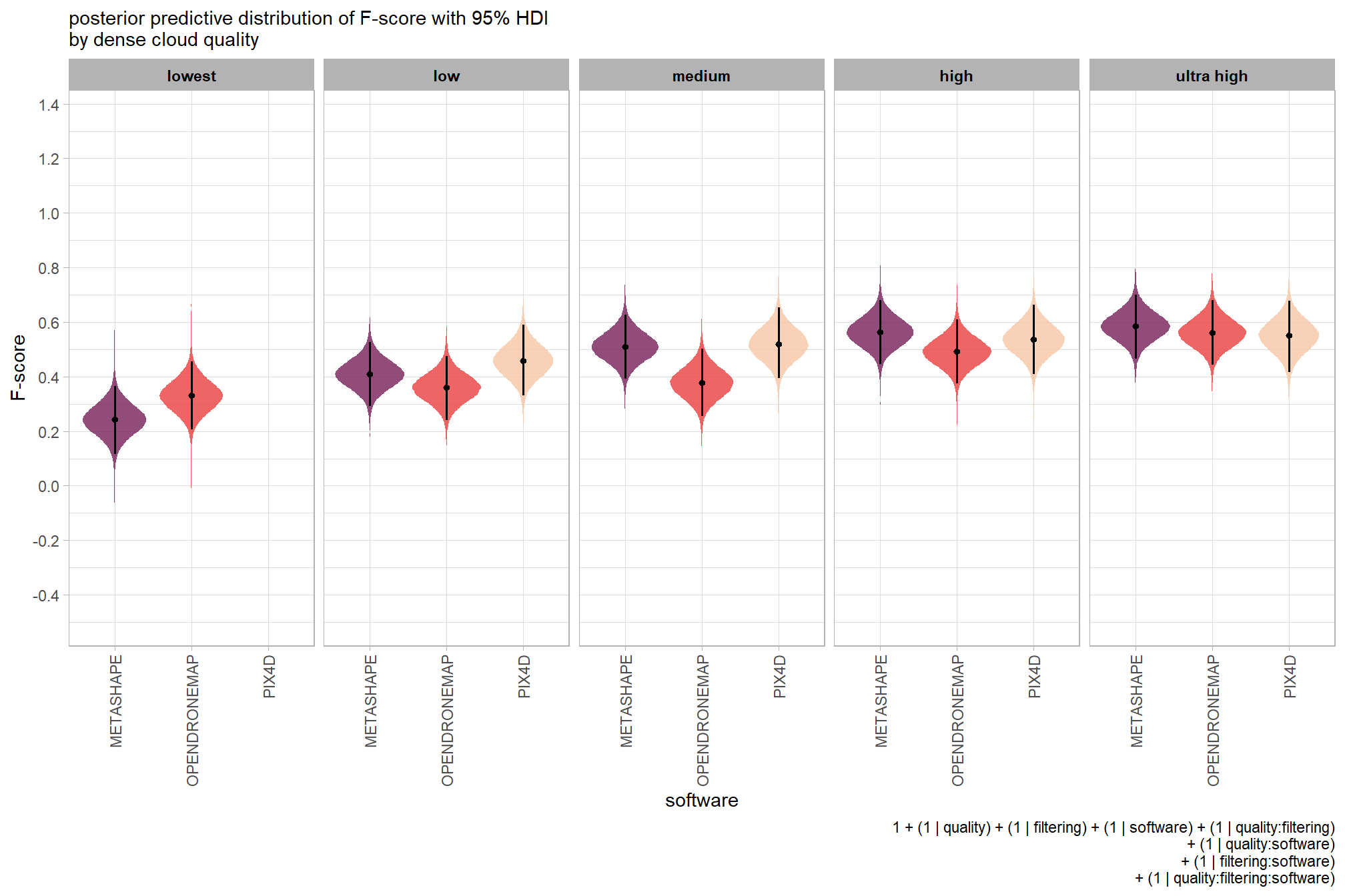
we can also make pairwise comparisons so long as we continue using tidybayes::add_epred_draws with the re_formula argument
brms_contrast_temp = qlty_sftwr_draws_temp %>%
  tidybayes::compare_levels(
    value
    , by = depth_maps_generation_quality
    , comparison =
      contrast_list[!stringr::str_detect(contrast_list, "lowest")]
      # contrast_list
  ) %>%
  dplyr::rename(contrast = depth_maps_generation_quality)

# separate contrast
brms_contrast_temp = brms_contrast_temp %>%
  dplyr::ungroup() %>%
  tidyr::separate_wider_delim(
    cols = contrast
    , delim = " - "
    , names = paste0(
      "sorter"
      , 1:(max(stringr::str_count(brms_contrast_temp$contrast, "-"))+1)
    )
    , too_few = "align_start"
    , cols_remove = F
  ) %>%
  dplyr::filter(sorter1!=sorter2) %>%
  dplyr::mutate(
    dplyr::across(
      tidyselect::starts_with("sorter")
      , .fns = function(x){factor(
        x, ordered = T
        , levels = levels(ptcld_validation_data$depth_maps_generation_quality)
      )}
    )
    , contrast = contrast %>%
      forcats::fct_reorder(
        paste0(as.numeric(sorter1), as.numeric(sorter2)) %>%
          as.numeric()
      )
  ) %>%
  # median_hdi summary for coloring
  dplyr::group_by(contrast, software) %>%
  make_contrast_vars()

# what?
brms_contrast_temp %>% dplyr::glimpse()
## Rows: 720,000
## Columns: 19
## Groups: contrast, software [18]
## $ software <chr> "METASHAPE", "METASHAPE", "METASHAPE", "METASHAPE", "…
## $ .chain <int> NA, NA, NA, NA, NA, NA, NA, NA, NA, NA, NA, NA, NA, N…
## $ .iteration <int> NA, NA, NA, NA, NA, NA, NA, NA, NA, NA, NA, NA, NA, N…
## $ .draw <int> 1, 2, 3, 4, 5, 6, 7, 8, 9, 10, 11, 12, 13, 14, 15, 16…
## $ sorter1 <ord> ultra high, ultra high, ultra high, ultra high, ultra…
## $ sorter2 <ord> high, high, high, high, high, high, high, high, high,…
## $ contrast <fct> ultra high - high, ultra high - high, ultra high - hi…
## $ value <dbl> 0.003195116, -0.019219782, 0.166484207, 0.109922877, …
## $ median_hdi_est <dbl> 0.02226909, 0.02226909, 0.02226909, 0.02226909, 0.022…
## $ median_hdi_lower <dbl> -0.09312331, -0.09312331, -0.09312331, -0.09312331, -…
## $ median_hdi_upper <dbl> 0.138316, 0.138316, 0.138316, 0.138316, 0.138316, 0.1…
## $ pr_gt_zero <chr> "65%", "65%", "65%", "65%", "65%", "65%", "65%", "65%…
## $ pr_lt_zero <chr> "35%", "35%", "35%", "35%", "35%", "35%", "35%", "35%…
## $ is_diff_dir <lgl> TRUE, FALSE, TRUE, TRUE, TRUE, TRUE, TRUE, TRUE, TRUE…
## $ pr_diff <dbl> 0.646325, 0.646325, 0.646325, 0.646325, 0.646325, 0.6…
## $ pr_diff_lab <chr> "Pr(ultra high>high)=65%", "Pr(ultra high>high)=65%",…
## $ pr_diff_lab_sm <chr> "Pr(>0)=65%", "Pr(>0)=65%", "Pr(>0)=65%", "Pr(>0)=65%…
## $ pr_diff_lab_pos <dbl> 0.1486897, 0.1486897, 0.1486897, 0.1486897, 0.1486897…
## $ sig_level <ord> <80%, <80%, <80%, <80%, <80%, <80%, <80%, <80%, <80%,…plot it
plt_contrast(
  brms_contrast_temp, caption_text = form_temp
  , y_axis_title = "quality"
  , facet = "software"
  , label_size = 2.2
  , x_expand = c(0,0.5)
) +
  labs(
    subtitle = "posterior predictive distribution of group constrasts with 95% & 50% HDI\nby software"
  )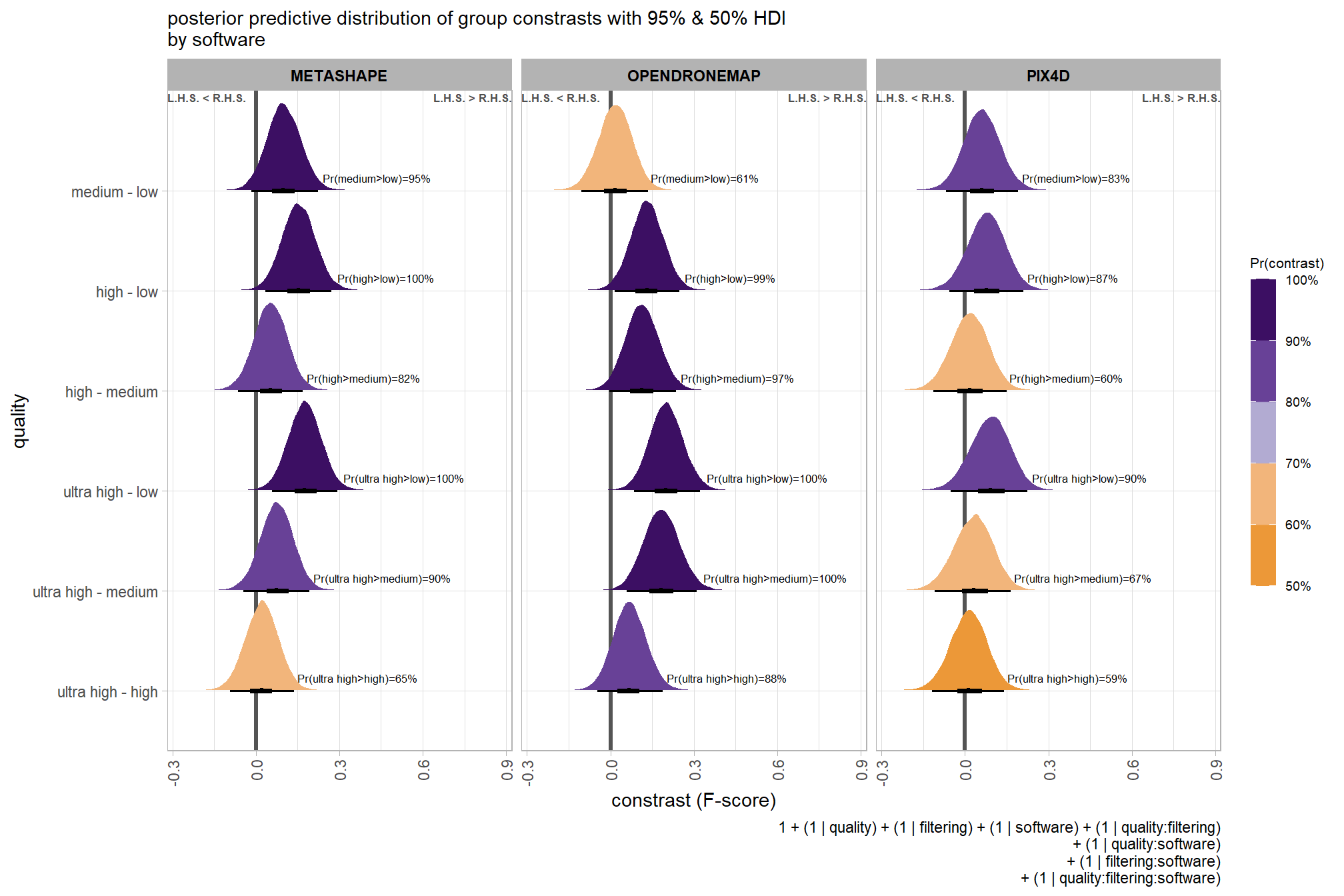
and summarize these contrasts
brms_contrast_temp %>%
  dplyr::group_by(contrast, software) %>%
  tidybayes::median_hdi(value) %>%
  dplyr::arrange(contrast, software) %>%
  dplyr::select(contrast, software, value, .lower, .upper) %>%

  kableExtra::kbl(
    digits = 2
    , caption = "brms::brm model: 95% HDI of the posterior predictive distribution of group constrasts"
    , col.names = c(
      "quality contrast"
      , "software"
      , "difference (F-score)"
      , "HDI low", "HDI high"
    )
  ) %>%
  kableExtra::kable_styling() %>%
kableExtra::scroll_box(height = "6in")| quality contrast | software | difference (F-score) | HDI low | HDI high |
|---|---|---|---|---|
| ultra high - high | METASHAPE | 0.02 | -0.09 | 0.14 |
| ultra high - high | OPENDRONEMAP | 0.07 | -0.05 | 0.19 |
| ultra high - high | PIX4D | 0.01 | -0.12 | 0.14 |
| ultra high - medium | METASHAPE | 0.08 | -0.04 | 0.19 |
| ultra high - medium | OPENDRONEMAP | 0.18 | 0.06 | 0.31 |
| ultra high - medium | PIX4D | 0.03 | -0.11 | 0.17 |
| ultra high - low | METASHAPE | 0.18 | 0.06 | 0.29 |
| ultra high - low | OPENDRONEMAP | 0.20 | 0.08 | 0.32 |
| ultra high - low | PIX4D | 0.09 | -0.05 | 0.22 |
| high - medium | METASHAPE | 0.05 | -0.07 | 0.17 |
| high - medium | OPENDRONEMAP | 0.11 | 0.00 | 0.23 |
| high - medium | PIX4D | 0.02 | -0.11 | 0.15 |
| high - low | METASHAPE | 0.15 | 0.03 | 0.27 |
| high - low | OPENDRONEMAP | 0.13 | 0.02 | 0.25 |
| high - low | PIX4D | 0.08 | -0.06 | 0.21 |
| medium - low | METASHAPE | 0.10 | -0.02 | 0.22 |
| medium - low | OPENDRONEMAP | 0.02 | -0.10 | 0.13 |
| medium - low | PIX4D | 0.06 | -0.07 | 0.19 |
let’s collapse across the filtering mode and software to compare the dense cloud quality setting effect.
In a hierarchical model structure, we have to make use of the re_formula argument within tidybayes::add_epred_draws
ptcld_validation_data %>%
  dplyr::distinct(depth_maps_generation_quality) %>%
  tidybayes::add_epred_draws(
    brms_f_mod3
    # this part is crucial
    , re_formula = ~ (1 | depth_maps_generation_quality)
  ) %>%
  dplyr::rename(value = .epred) %>%
  # plot
  ggplot(
    mapping = aes(
      x = value, y = depth_maps_generation_quality
      , fill = depth_maps_generation_quality
    )
  ) +
    tidybayes::stat_halfeye(
      point_interval = median_hdi, .width = .95
      , interval_color = "gray66"
      , shape = 21, point_color = "gray66", point_fill = "black"
      , justification = -0.01
    ) +
    scale_fill_viridis_d(option = "inferno", drop = F) +
    scale_x_continuous(breaks = scales::extended_breaks(n=8)) +
    labs(
      y = "quality", x = "F-score"
      , subtitle = "posterior predictive distribution of F-score with 95% HDI"
      , caption = form_temp
    ) +
    theme_light() +
    theme(legend.position = "none")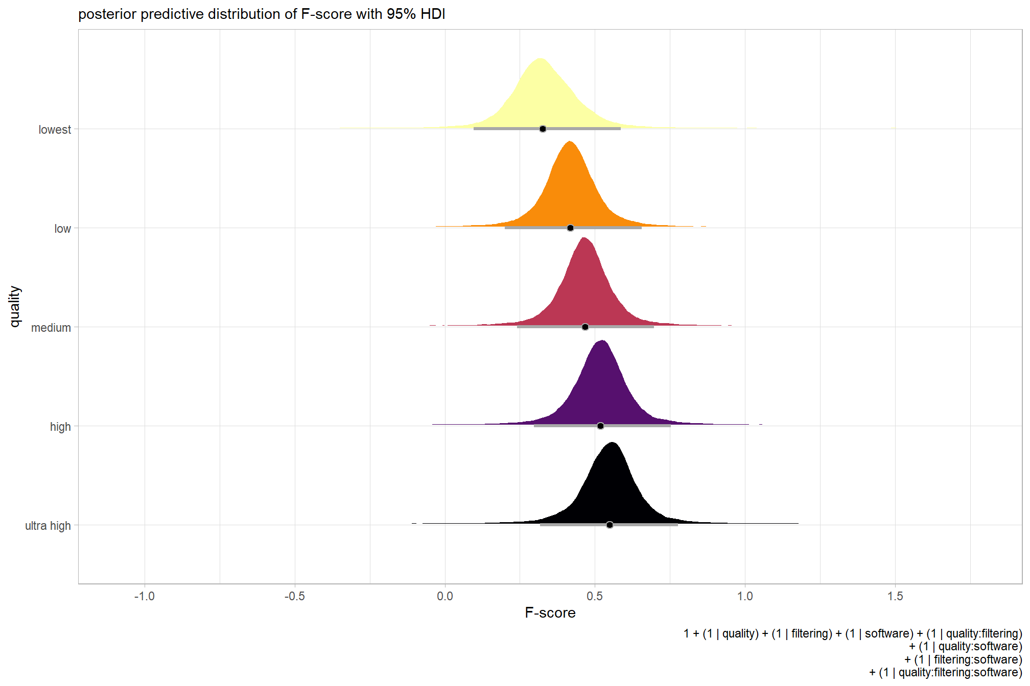
let’s compare these results to the results from our one nominal predictor model above and two nominal predictor model
ptcld_validation_data %>%
  dplyr::distinct(depth_maps_generation_quality) %>%
  tidybayes::add_epred_draws(
    brms_f_mod3
    # this part is crucial
    , re_formula = ~ (1 | depth_maps_generation_quality)
  ) %>%
  dplyr::mutate(value = .epred, src = "brms_f_mod3") %>%
  dplyr::bind_rows(
    ptcld_validation_data %>%
      dplyr::distinct(depth_maps_generation_quality) %>%
      tidybayes::add_epred_draws(
        brms_f_mod2
        # this part is crucial
        , re_formula = ~ (1 | depth_maps_generation_quality)
      ) %>%
      dplyr::mutate(value = .epred, src = "brms_f_mod2")
    , ptcld_validation_data %>%
      dplyr::distinct(depth_maps_generation_quality) %>%
      tidybayes::add_epred_draws(brms_f_mod1) %>%
      dplyr::mutate(value = .epred, src = "brms_f_mod1")
  ) %>%
  ggplot(mapping = aes(y = src, x = value, color = src, group = src)) +
  tidybayes::stat_pointinterval(position = "dodge") +
  facet_grid(rows = vars(depth_maps_generation_quality), switch = "y") +
  scale_y_discrete(NULL, breaks = NULL) +
  scale_color_manual(values = viridis::turbo(n = 6, begin = 0.2, end = 0.8)[1:3]) +
  labs(
    y = "", x = "F-score"
    , color = "model"
  ) +
  theme_light() +
  theme(legend.position = "top", strip.text = element_text(color = "black", face = "bold"))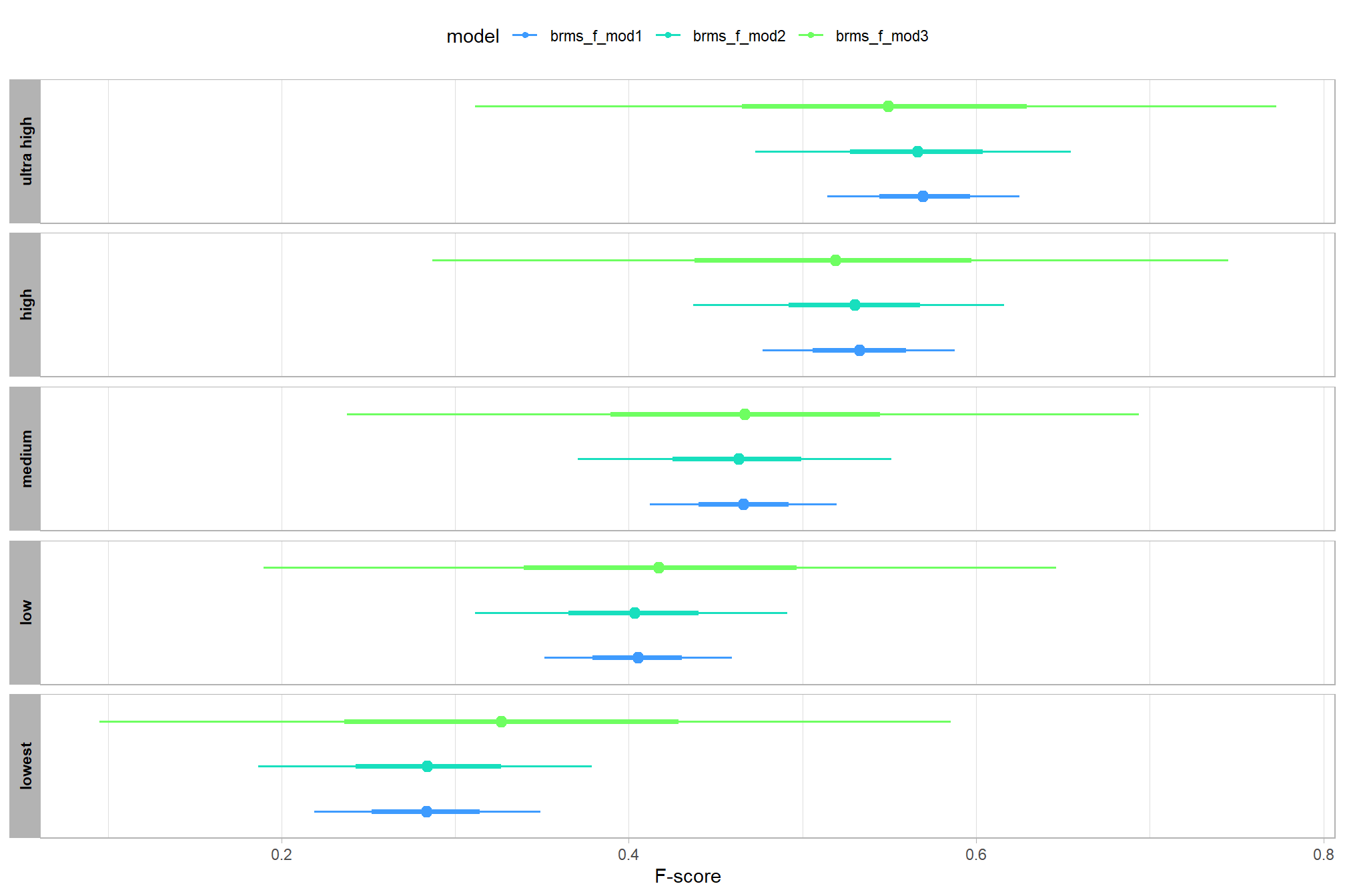
let’s also collapse across the dense cloud quality and software to compare the filtering mode setting effect.
In a hierarchical model structure, we have to make use of the re_formula argument within tidybayes::add_epred_draws
ptcld_validation_data %>%
  dplyr::distinct(depth_maps_generation_filtering_mode) %>%
  tidybayes::add_epred_draws(
    brms_f_mod3
    # this part is crucial
    , re_formula = ~ (1 | depth_maps_generation_filtering_mode)
  ) %>%
  dplyr::rename(value = .epred) %>%
  # plot
  ggplot(
    mapping = aes(
      x = value, y = depth_maps_generation_filtering_mode
      , fill = depth_maps_generation_filtering_mode
    )
  ) +
    tidybayes::stat_halfeye(
      point_interval = median_hdi, .width = .95
      , interval_color = "gray66"
      , shape = 21, point_color = "gray66", point_fill = "black"
      , justification = -0.01
    ) +
    scale_fill_viridis_d(option = "plasma", drop = F) +
    scale_x_continuous(breaks = scales::extended_breaks(n=8)) +
    labs(
      y = "filtering mode", x = "F-score"
      , subtitle = "posterior predictive distribution of F-score with 95% HDI"
      , caption = form_temp
    ) +
    theme_light() +
    theme(legend.position = "none")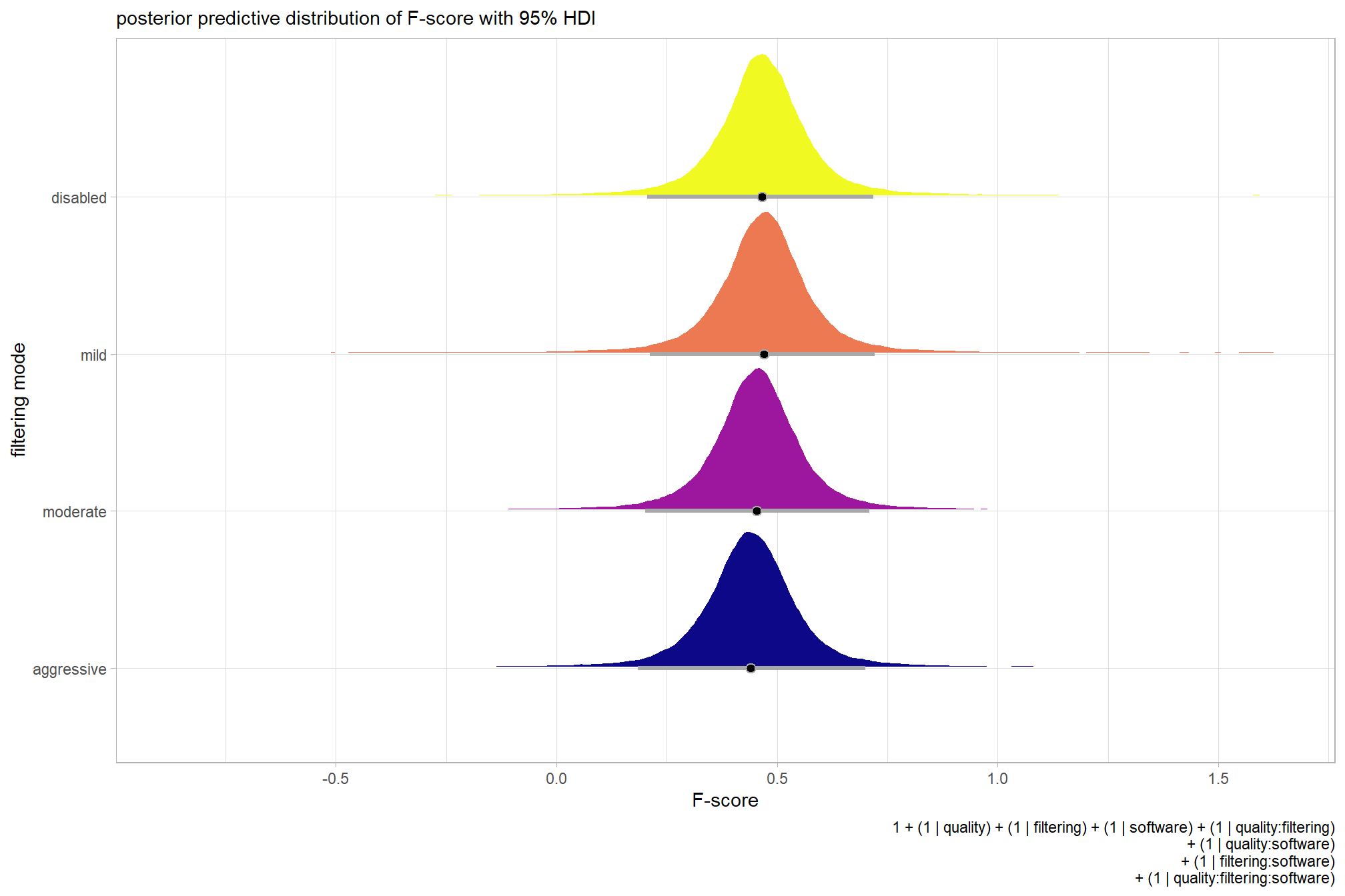
let’s compare these results to the results from our two nominal predictor model above
ptcld_validation_data %>%
  dplyr::distinct(depth_maps_generation_filtering_mode) %>%
  tidybayes::add_epred_draws(
    brms_f_mod3
    # this part is crucial
    , re_formula = ~ (1 | depth_maps_generation_filtering_mode)
  ) %>%
  dplyr::mutate(value = .epred, src = "brms_f_mod3") %>%
  dplyr::bind_rows(
    ptcld_validation_data %>%
      dplyr::distinct(depth_maps_generation_filtering_mode) %>%
      tidybayes::add_epred_draws(
        brms_f_mod2
        # this part is crucial
        , re_formula = ~ (1 | depth_maps_generation_filtering_mode)
      ) %>%
      dplyr::mutate(value = .epred, src = "brms_f_mod2")
  ) %>%
  ggplot(mapping = aes(y = src, x = value, color = src, group = src)) +
  tidybayes::stat_pointinterval(position = "dodge") +
  facet_grid(rows = vars(depth_maps_generation_filtering_mode), switch = "y") +
  scale_y_discrete(NULL, breaks = NULL) +
  scale_color_manual(values = viridis::turbo(n = 6, begin = 0.2, end = 0.8)[2:3]) +
  labs(
    y = "filtering mode", x = "F-score"
    , color = "model"
  ) +
  theme_light() +
  theme(legend.position = "top", strip.text = element_text(color = "black", face = "bold"))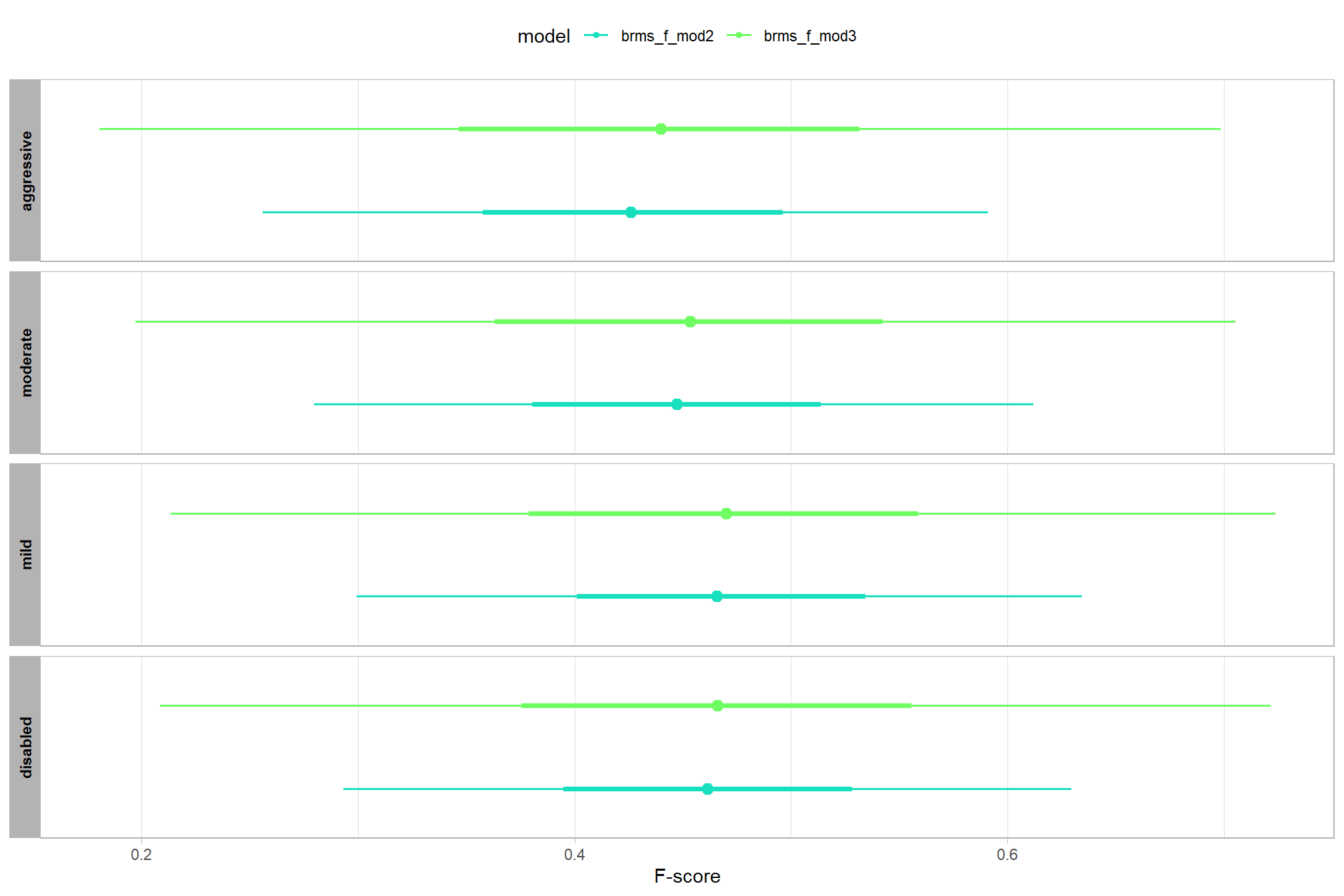
to address one of our main questions, let’s also collapse across the dense cloud quality and filtering mode setting to compare the software effect.
In a hierarchical model structure, we have to make use of the re_formula argument within tidybayes::add_epred_draws
ptcld_validation_data %>%
  dplyr::distinct(software) %>%
  tidybayes::add_epred_draws(
    brms_f_mod3
    # this part is crucial
    , re_formula = ~ (1 | software)
  ) %>%
  dplyr::rename(value = .epred) %>%
  # plot
  ggplot(
    mapping = aes(
      x = value, y = software
      , fill = software
    )
  ) +
    tidybayes::stat_halfeye(
      point_interval = median_hdi, .width = .95
      , interval_color = "gray66"
      , shape = 21, point_color = "gray66", point_fill = "black"
      , justification = -0.01
    ) +
    scale_fill_viridis_d(option = "rocket", begin = 0.3, end = 0.9, drop = F) +
    scale_x_continuous(breaks = scales::extended_breaks(n=8)) +
    labs(
      y = "software", x = "F-score"
      , subtitle = "posterior predictive distribution of F-score with 95% HDI"
      , caption = form_temp
    ) +
    theme_light() +
    theme(legend.position = "none")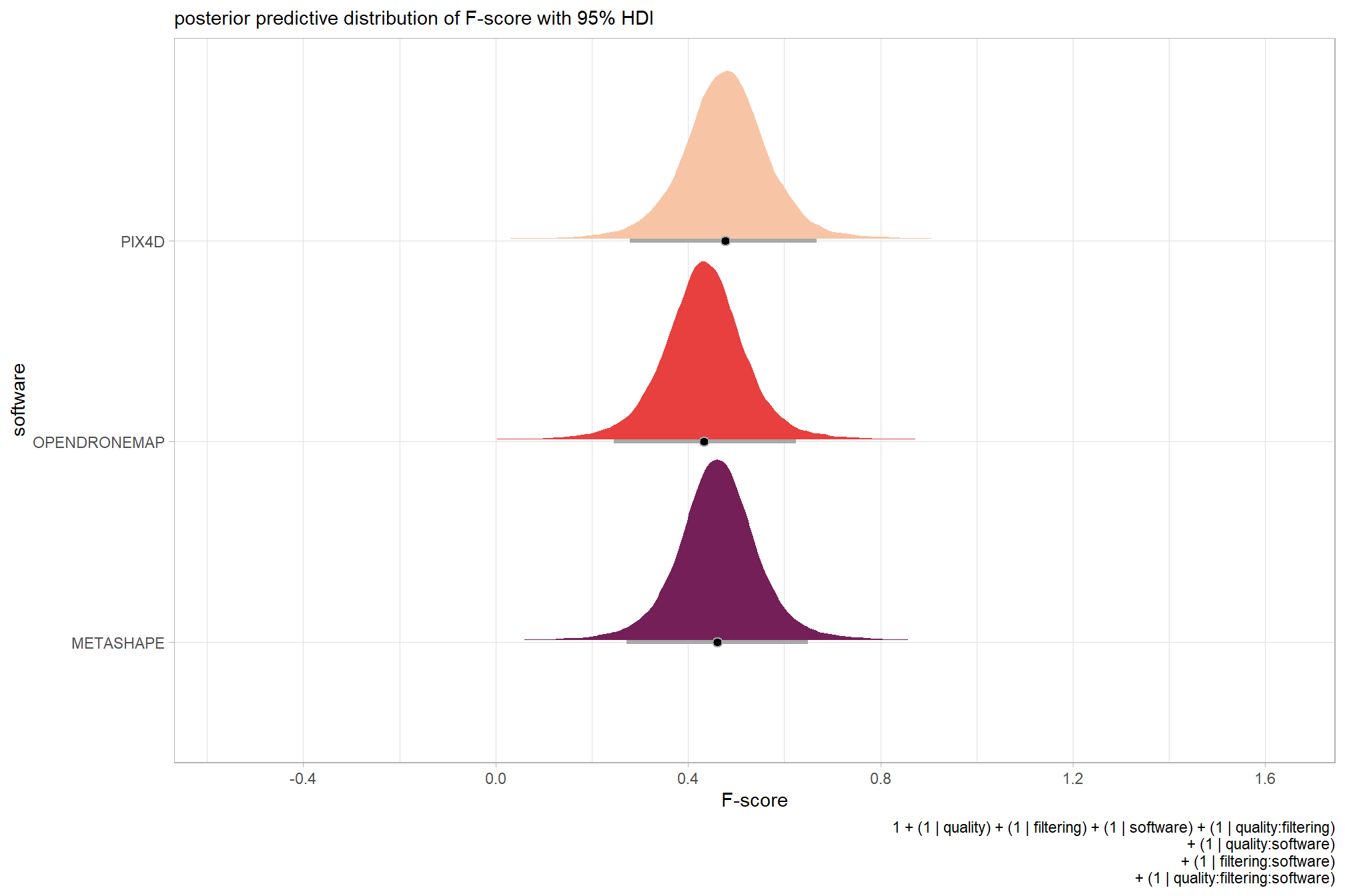
Finally, we can quantify the variation in F-score by comparing the \(\sigma\) posteriors.
# extract the posterior draws
brms::as_draws_df(brms_f_mod3) %>%
  dplyr::select(c(sigma,tidyselect::starts_with("sd_"))) %>%
  tidyr::pivot_longer(dplyr::everything()) %>%
  # dplyr::group_by(name) %>%
  # tidybayes::median_hdi(value) %>%
  dplyr::mutate(
    name = name %>%
      stringr::str_replace_all("depth_maps_generation_quality", "quality") %>%
      stringr::str_replace_all("depth_maps_generation_filtering_mode", "filtering") %>%
      forcats::fct_reorder(value)
  ) %>%
# plot
  ggplot(aes(x = value, y = name)) +
  tidybayes::stat_dotsinterval(
    point_interval = median_hdi, .width = .95
    , justification = -0.04
    , shape = 21 #, point_size = 3
    , quantiles = 100
  ) +
  labs(x = "", y = "", caption = form_temp) +
  theme_light()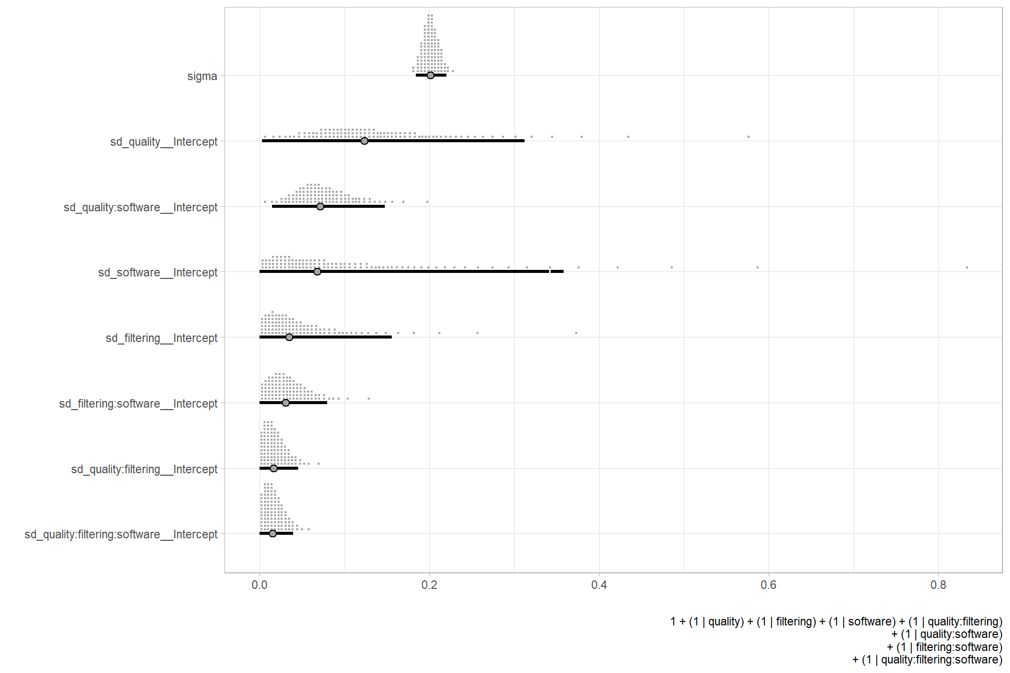
and perform model selection via information criteria with the brms::loo_compare() function
brms_f_mod3 = brms::add_criterion(brms_f_mod3, criterion = c("loo", "waic"))
brms::loo_compare(brms_f_mod1, brms_f_mod2, brms_f_mod3, criterion = "loo")
## elpd_diff se_diff
## brms_f_mod3 0.0 0.0
## brms_f_mod1 -0.3 3.8
## brms_f_mod2 -2.0 3.66.6 Three Nominal Predictors + site effects
Now, we’ll add the average deflection from the baseline (i.e. the “grand mean”) due to study site (i.e. the “subjects” in our data). The main effect for the study site will be added to our model with the combined influence of the depth map generation quality, the depth map filtering, and the software on the F-score.
In the model we use below, the study site is modeled as a “random effect.” Hobbs et al. (2024) describe a similar model:
It is important to understand that fitting treatment intercepts and slopes as random rather than fixed means that our inference applied to all possible sites suitable for [inclusion in the study]. In contrast, assuming fixed effects of treatment would dramatically reduce the uncertainty about those effects, but would constrain inference to the four sites that we studied. (p. 13)
6.6.1 Summary Statistics
Each study site contributes one observation per dense cloud quality, filtering mode, and software. That is, a row in the underlying data is unique by study site, software, dense cloud quality, and filtering mode.
identical(
  # base data
  nrow(ptcld_validation_data)
  # distinct group
  , ptcld_validation_data %>%
    dplyr::distinct(
      study_site
      , software
      , depth_maps_generation_quality
      , depth_maps_generation_filtering_mode
    ) %>%
    nrow()
)
## [1] TRUE6.6.2 Bayesian
Kruschke (2015) describes the Hierarchical Bayesian approach to describe groups of metric data with multiple nominal predictors when every subject (“study site” in our research) only contributes one observation per cell/condition:
\[\begin{align*} y = & \; \beta_0 \\ & + \overrightarrow \beta_1 \overrightarrow x_1 + \overrightarrow \beta_2 \overrightarrow x_2 + \overrightarrow \beta_{1 \times 2} \overrightarrow x_{1 \times 2} \\ & + \overrightarrow \beta_S \overrightarrow x_S \end{align*}\]
In other words, we assume a main effect of subject, but no interaction of subject with other predictors. In this model, the subject effect (deflection) is constant across treatments, and the treatment effects (deflections) are constant across subjects. Notice that the model makes no requirement that every subject contributes a datum to every condition. Indeed, the model allows zero or multiple data per subject per condition. Bayesian estimation makes no assumptions or requirements that the design is balanced (i.e., has equal numbers of measurement in each cell). (p. 608)
and see section 20 from Kurz’s ebook supplement
The metric predicted variable with three nominal predictor variables and subject-level effects model has the form:
\[\begin{align*} y_{i} \sim & \operatorname{Normal} \bigl(\mu_{i}, \sigma_{y} \bigr) \\ \mu_{i} = & \beta_0 \\ & + \sum_{j} \beta_{1[j]} x_{1[j]} + \sum_{k} \beta_{2[k]} x_{2[k]} + \sum_{f} \beta_{3[f]} x_{3[f]} + \sum_{s} \beta_{4[s]} x_{4[s]} \\ & + \sum_{j,k} \beta_{1\times2[j,k]} x_{1\times2[j,k]} + \sum_{j,f} \beta_{1\times3[j,f]} x_{1\times3[j,f]} + \sum_{k,f} \beta_{2\times3[k,f]} x_{2\times3[k,f]} \\ & + \sum_{j,k,f} \beta_{1\times2\times3[j,k,f]} x_{1\times2\times3[j,k,f]} \\ \beta_{0} \sim & \operatorname{Normal}(0,100) \\ \beta_{1[j]} \sim & \operatorname{Normal}(0,\sigma_{\beta_{1}}) \\ \beta_{2[k]} \sim & \operatorname{Normal}(0,\sigma_{\beta_{2}}) \\ \beta_{3[f]} \sim & \operatorname{Normal}(0,\sigma_{\beta_{3}}) \\ \beta_{4[s]} \sim & \operatorname{Normal}(0,\sigma_{\beta_{4}}) \\ \beta_{1\times2[j,k]} \sim & \operatorname{Normal}(0,\sigma_{\beta_{1\times2}}) \\ \beta_{1\times3[j,f]} \sim & \operatorname{Normal}(0,\sigma_{\beta_{1\times3}}) \\ \beta_{2\times3[k,f]} \sim & \operatorname{Normal}(0,\sigma_{\beta_{2\times3}}) \\ \sigma_{\beta_{1}} \sim & \operatorname{Gamma}(1.28,0.005) \\ \sigma_{\beta_{2}} \sim & \operatorname{Gamma}(1.28,0.005) \\ \sigma_{\beta_{3}} \sim & \operatorname{Gamma}(1.28,0.005) \\ \sigma_{\beta_{4}} \sim & \operatorname{Gamma}(1.28,0.005) \\ \sigma_{\beta_{1\times2}} \sim & \operatorname{Gamma}(1.28,0.005) \\ \sigma_{\beta_{1\times3}} \sim & \operatorname{Gamma}(1.28,0.005) \\ \sigma_{\beta_{2\times3}} \sim & \operatorname{Gamma}(1.28,0.005) \\ \sigma_{y} \sim & {\sf Cauchy} (0,109) \\ \end{align*}\]
, where \(j\) is the depth map generation quality setting corresponding to observation \(i\), \(k\) is the depth map filtering mode setting corresponding to observation \(i\), \(f\) is the processing software corresponding to observation \(i\), and \(s\) is the study site corresponding to observation \(i\)
for this model, we’ll define the priors following Kurz:
# from Kurz:
gamma_a_b_from_omega_sigma = function(mode, sd) {
  if (mode <= 0) stop("mode must be > 0")
  if (sd   <= 0) stop("sd must be > 0")
  rate = (mode + sqrt(mode^2 + 4 * sd^2)) / (2 * sd^2)
  shape = 1 + mode * rate
  return(list(shape = shape, rate = rate))
}

mean_y_temp = mean(ptcld_validation_data$f_score)
sd_y_temp   = sd(ptcld_validation_data$f_score)

omega_temp = sd_y_temp / 2
sigma_temp = 2 * sd_y_temp

s_r_temp = gamma_a_b_from_omega_sigma(mode = omega_temp, sd = sigma_temp)

stanvars_temp =
  brms::stanvar(mean_y_temp,    name = "mean_y") +
  brms::stanvar(sd_y_temp,      name = "sd_y") +
  brms::stanvar(s_r_temp$shape, name = "alpha") +
  brms::stanvar(s_r_temp$rate,  name = "beta")
Now fit the model.
brms_f_mod4 = brms::brm(
  formula = f_score ~
    # baseline
    1 +
    # main effects
    (1 | depth_maps_generation_quality) +
    (1 | depth_maps_generation_filtering_mode) +
    (1 | software) +
    (1 | study_site) + # only fitting main effects of site and not interactions
    # two-way interactions
    (1 | depth_maps_generation_quality:depth_maps_generation_filtering_mode) +
    (1 | depth_maps_generation_quality:software) +
    (1 | depth_maps_generation_filtering_mode:software) +
    # three-way interactions
    (1 | depth_maps_generation_quality:depth_maps_generation_filtering_mode:software)
  , data = ptcld_validation_data
  , family = brms::brmsfamily(family = "gaussian")
  , iter = 20000, warmup = 10000, chains = 4
  , control = list(adapt_delta = 0.999, max_treedepth = 13)
  , cores = round(parallel::detectCores()/2)
  , prior = c(
    brms::prior(normal(mean_y, sd_y * 5), class = "Intercept")
    , brms::prior(gamma(alpha, beta), class = "sd")
    , brms::prior(cauchy(0, sd_y), class = "sigma")
  )
  , stanvars = stanvars_temp
  , file = paste0(rootdir, "/fits/brms_f_mod4")
)
check the trace plots for problems with convergence of the Markov chains
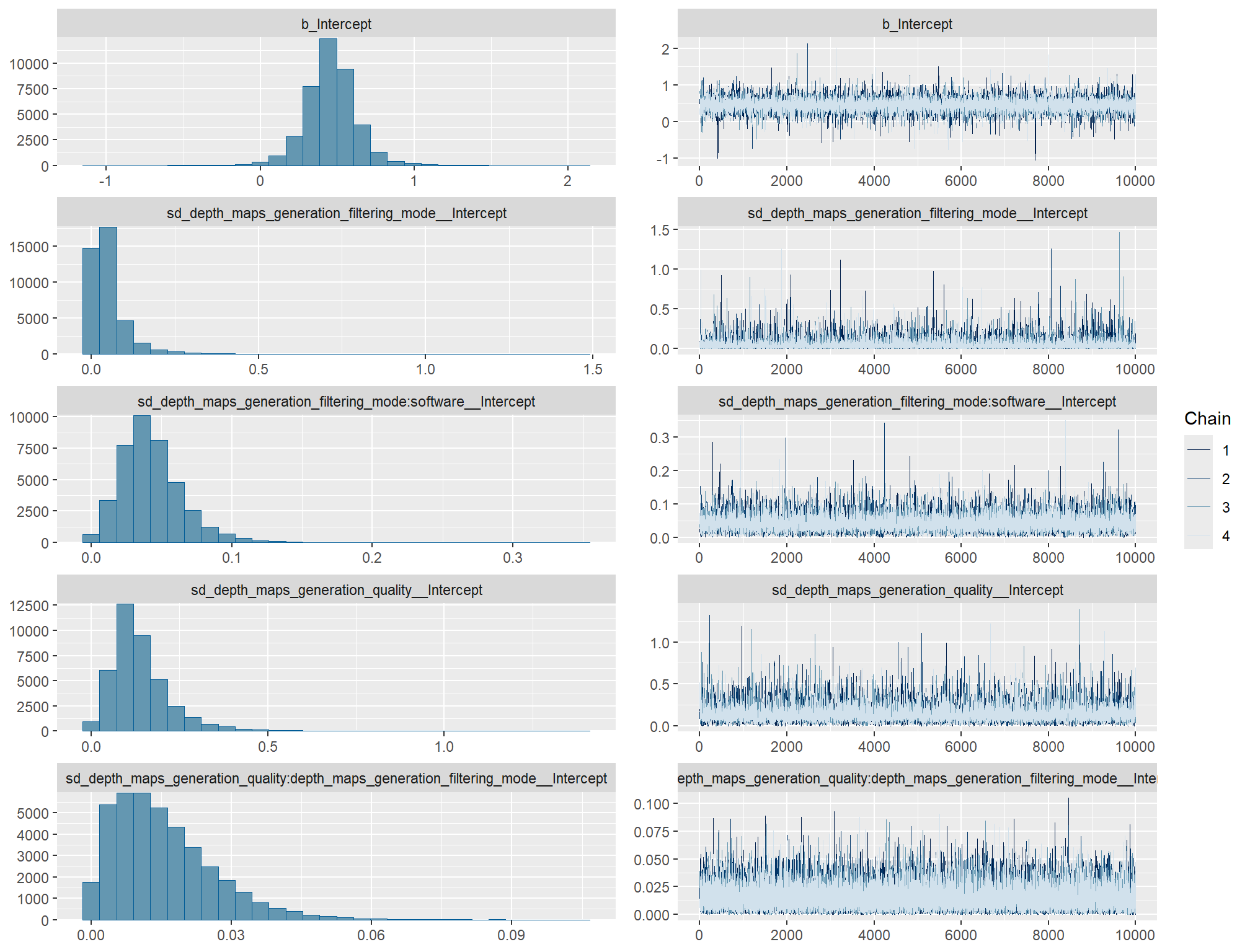
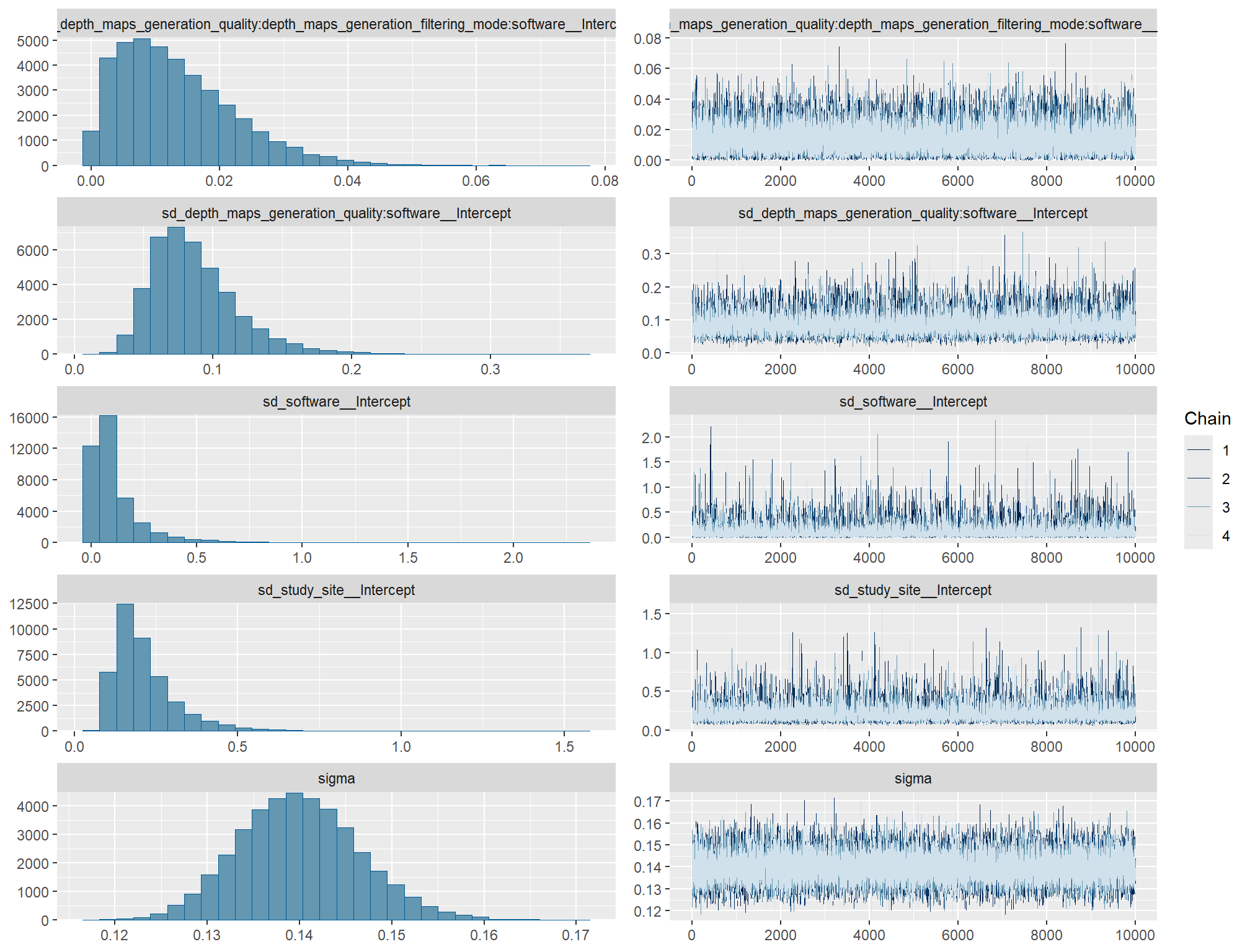
check the prior distributions
# check priors
brms::prior_summary(brms_f_mod4) %>%
  kableExtra::kbl() %>%
kableExtra::kable_styling()| prior | class | coef | group | resp | dpar | nlpar | lb | ub | source |
|---|---|---|---|---|---|---|---|---|---|
| normal(mean_y, sd_y * 5) | Intercept | user | |||||||
| gamma(alpha, beta) | sd | 0 | user | ||||||
| sd | depth_maps_generation_filtering_mode | default | |||||||
| sd | Intercept | depth_maps_generation_filtering_mode | default | ||||||
| sd | depth_maps_generation_filtering_mode:software | default | |||||||
| sd | Intercept | depth_maps_generation_filtering_mode:software | default | ||||||
| sd | depth_maps_generation_quality | default | |||||||
| sd | Intercept | depth_maps_generation_quality | default | ||||||
| sd | depth_maps_generation_quality:depth_maps_generation_filtering_mode | default | |||||||
| sd | Intercept | depth_maps_generation_quality:depth_maps_generation_filtering_mode | default | ||||||
| sd | depth_maps_generation_quality:depth_maps_generation_filtering_mode:software | default | |||||||
| sd | Intercept | depth_maps_generation_quality:depth_maps_generation_filtering_mode:software | default | ||||||
| sd | depth_maps_generation_quality:software | default | |||||||
| sd | Intercept | depth_maps_generation_quality:software | default | ||||||
| sd | software | default | |||||||
| sd | Intercept | software | default | ||||||
| sd | study_site | default | |||||||
| sd | Intercept | study_site | default | ||||||
| cauchy(0, sd_y) | sigma | 0 | user |
The brms::brm model summary
We won’t clutter the output here but this can be run if you are following along on your own
brms_f_mod4 %>%
  brms::posterior_summary() %>%
  as.data.frame() %>%
  tibble::rownames_to_column(var = "parameter") %>%
  dplyr::rename_with(tolower) %>%
  dplyr::filter(
    stringr::str_starts(parameter, "b_")
    | stringr::str_starts(parameter, "r_")
    | stringr::str_starts(parameter, "sd_")
    | parameter == "sigma"
  ) %>%
  dplyr::mutate(
    parameter = parameter %>%
      stringr::str_replace_all("depth_maps_generation_quality", "quality") %>%
      stringr::str_replace_all("depth_maps_generation_filtering_mode", "filtering")
  ) %>%
  kableExtra::kbl(digits = 2, caption = "Bayesian 3 nominal predictors + study site effects for F-score") %>%
  kableExtra::kable_styling() %>%
  kableExtra::scroll_box(height = "6in")
We can look at the model noise standard deviation \(\sigma_y\)
# get formula
form_temp = brms_f_mod4$formula$formula[3] %>%
  as.character() %>% get_frmla_text() %>%
  stringr::str_replace_all("depth_maps_generation_quality", "quality") %>%
  stringr::str_replace_all("depth_maps_generation_filtering_mode", "filtering")
# extract the posterior draws
brms::as_draws_df(brms_f_mod4) %>%
# plot
  ggplot(aes(x = sigma, y = 0)) +
  tidybayes::stat_dotsinterval(
    point_interval = median_hdi, .width = .95
    , justification = -0.04
    , shape = 21, point_size = 3
    , quantiles = 100
  ) +
  scale_y_continuous(NULL, breaks = NULL) +
  labs(
    x = latex2exp::TeX("$\\sigma_y$")
    , caption = form_temp
  ) +
  theme_light()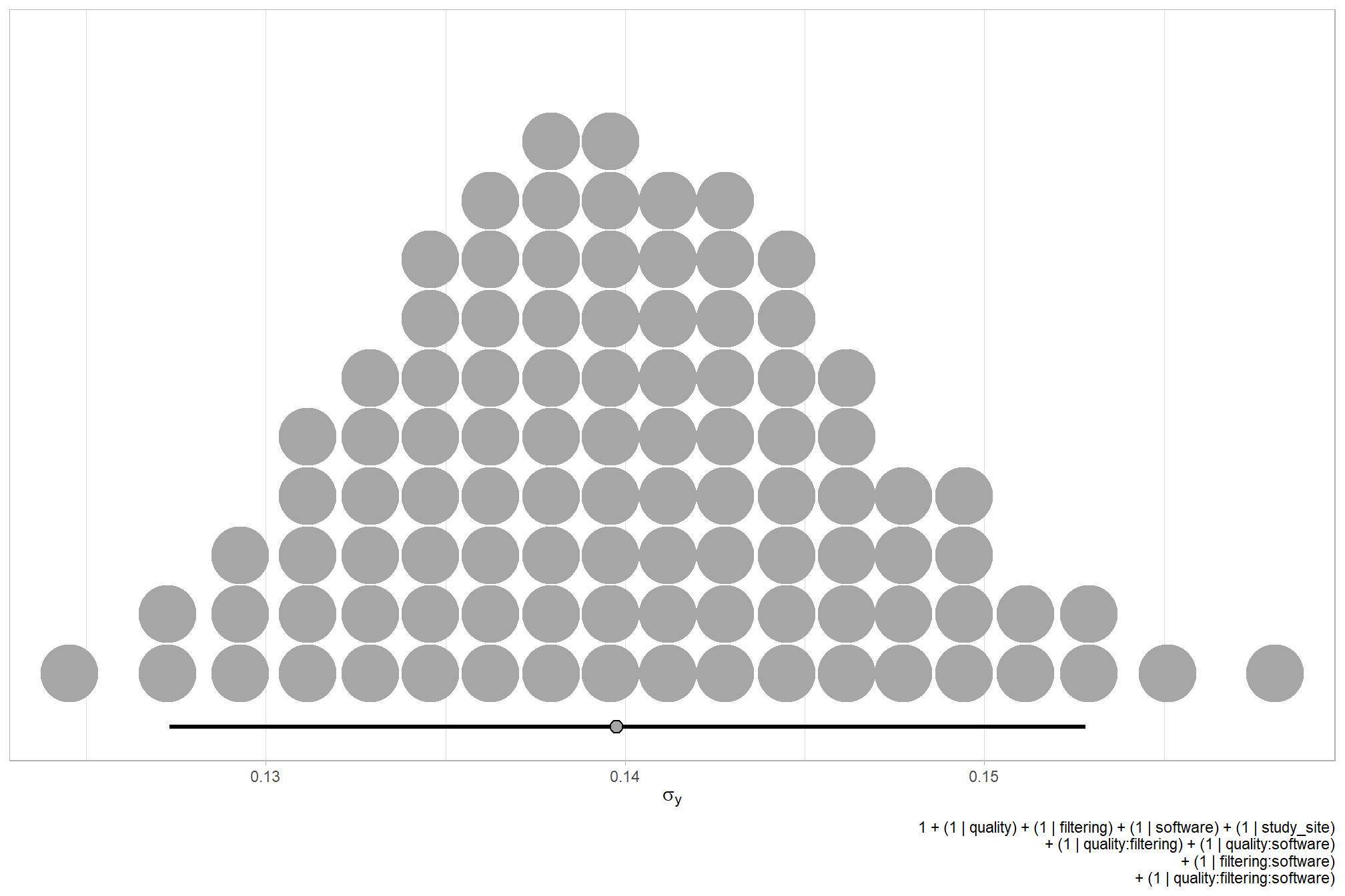
how is it compared to our other models?
# how is it compared to our other models?
dplyr::bind_rows(
    brms::as_draws_df(brms_f_mod1) %>% tidybayes::median_hdi(sigma) %>% dplyr::mutate(model = "one nominal predictor")
    , brms::as_draws_df(brms_f_mod2) %>% tidybayes::median_hdi(sigma) %>% dplyr::mutate(model = "two nominal predictor")
    , brms::as_draws_df(brms_f_mod3) %>% tidybayes::median_hdi(sigma) %>% dplyr::mutate(model = "three nominal predictor")
    , brms::as_draws_df(brms_f_mod4) %>% tidybayes::median_hdi(sigma) %>% dplyr::mutate(model = "three+site nominal predictor")
  ) %>%
  dplyr::relocate(model) %>%
  kableExtra::kbl(digits = 2, caption = "brms::brm model noise standard deviation comparison") %>%
kableExtra::kable_styling()| model | sigma | .lower | .upper | .width | .point | .interval |
|---|---|---|---|---|---|---|
| one nominal predictor | 0.21 | 0.19 | 0.23 | 0.95 | median | hdi |
| two nominal predictor | 0.21 | 0.19 | 0.23 | 0.95 | median | hdi |
| three nominal predictor | 0.20 | 0.18 | 0.22 | 0.95 | median | hdi |
| three+site nominal predictor | 0.14 | 0.13 | 0.15 | 0.95 | median | hdi |
plot the posterior predictive distributions of the conditional means with the median F-score and the 95% highest posterior density interval (HDI)
Note that how within tidybayes::add_epred_draws, we used the re_formula argument to average over the random effects of study_site (i.e., we left (1 | study_site) out of the formula) and software (i.e., we left (1 | software) and its interactions out of the formula).
qlty_filter_draws_temp =
  ptcld_validation_data %>%
    dplyr::distinct(depth_maps_generation_quality, depth_maps_generation_filtering_mode) %>%
    tidybayes::add_epred_draws(
      brms_f_mod4, allow_new_levels = T
      # this part is crucial
      , re_formula = ~ (1 | depth_maps_generation_quality) +
        (1 | depth_maps_generation_filtering_mode) +
        (1 | depth_maps_generation_quality:depth_maps_generation_filtering_mode)
    ) %>%
    dplyr::rename(value = .epred)
# hey plot
qlty_filter_draws_temp %>%
  dplyr::mutate(depth_maps_generation_quality = depth_maps_generation_quality %>% forcats::fct_rev()) %>%
  # plot
  ggplot(
    mapping = aes(
      y = value, x = depth_maps_generation_filtering_mode
      , fill = depth_maps_generation_filtering_mode
    )
  ) +
    tidybayes::stat_eye(
      point_interval = median_hdi, .width = .95
      , slab_alpha = 0.8
      , interval_color = "black", linewidth = 1
      , point_color = "black", point_fill = "black", point_size = 1
    ) +
    scale_fill_viridis_d(option = "plasma", drop = F) +
    scale_y_continuous(breaks = scales::extended_breaks(n=10)) +
    facet_grid(cols = vars(depth_maps_generation_quality)) +
    labs(
      x = "filtering mode", y = "F-score"
      , subtitle = "posterior predictive distribution of F-score with 95% HDI\nby dense cloud quality"
      , fill = "Filtering Mode"
      , caption = form_temp
    ) +
    theme_light() +
    theme(
      legend.position = "none"
      , legend.direction  = "horizontal"
      , axis.text.x = element_text(angle = 90, vjust = 0.5, hjust = 1)
      , strip.text = element_text(color = "black", face = "bold")
) 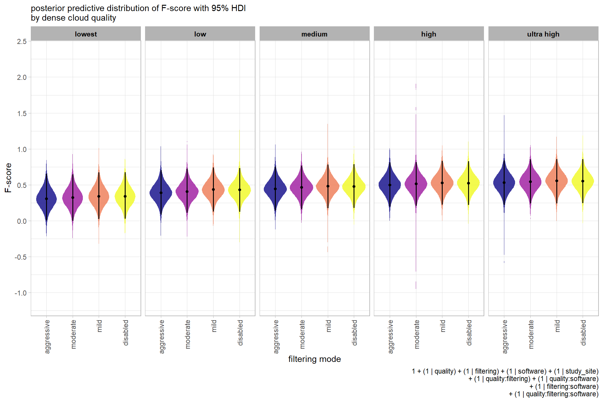
we can also make pairwise comparisons so long as we continue using tidybayes::add_epred_draws with the re_formula argument
brms_contrast_temp = qlty_filter_draws_temp %>%
    tidybayes::compare_levels(
      value
      , by = depth_maps_generation_quality
      , comparison =
        contrast_list
        # tidybayes::emmeans_comparison("revpairwise")
        #"pairwise"
    ) %>%
    dplyr::rename(contrast = depth_maps_generation_quality)

# separate contrast
brms_contrast_temp = brms_contrast_temp %>%
  dplyr::ungroup() %>%
  tidyr::separate_wider_delim(
    cols = contrast
    , delim = " - "
    , names = paste0(
        "sorter"
        , 1:(max(stringr::str_count(brms_contrast_temp$contrast, "-"))+1)
      )
    , too_few = "align_start"
    , cols_remove = F
  ) %>%
  dplyr::filter(sorter1!=sorter2) %>%
  dplyr::mutate(
    dplyr::across(
      tidyselect::starts_with("sorter")
      , .fns = function(x){factor(
        x, ordered = T
        , levels = levels(ptcld_validation_data$depth_maps_generation_quality)
      )}
    )
    , contrast = contrast %>%
      forcats::fct_reorder(
        paste0(as.numeric(sorter1), as.numeric(sorter2)) %>%
        as.numeric()
      )
    , depth_maps_generation_filtering_mode = depth_maps_generation_filtering_mode %>%
      factor(
        levels = levels(ptcld_validation_data$depth_maps_generation_filtering_mode)
        , ordered = T
      )
  ) %>%
  # median_hdi summary for coloring
  dplyr::group_by(contrast,depth_maps_generation_filtering_mode) %>%
  make_contrast_vars()

# what?
brms_contrast_temp %>% dplyr::glimpse()
## Rows: 1,600,000
## Columns: 19
## Groups: contrast, depth_maps_generation_filtering_mode [40]
## $ depth_maps_generation_filtering_mode <ord> aggressive, aggressive, aggressiv…
## $ .chain <int> NA, NA, NA, NA, NA, NA, NA, NA, N…
## $ .iteration <int> NA, NA, NA, NA, NA, NA, NA, NA, N…
## $ .draw <int> 1, 2, 3, 4, 5, 6, 7, 8, 9, 10, 11…
## $ sorter1 <ord> ultra high, ultra high, ultra hig…
## $ sorter2 <ord> high, high, high, high, high, hig…
## $ contrast <fct> ultra high - high, ultra high - h…
## $ value <dbl> 0.117091583, 0.258056922, -0.0900…
## $ median_hdi_est <dbl> 0.02936285, 0.02936285, 0.0293628…
## $ median_hdi_lower <dbl> -0.1084457, -0.1084457, -0.108445…
## $ median_hdi_upper <dbl> 0.174886, 0.174886, 0.174886, 0.1…
## $ pr_gt_zero <chr> "68%", "68%", "68%", "68%", "68%"…
## $ pr_lt_zero <chr> "32%", "32%", "32%", "32%", "32%"…
## $ is_diff_dir <lgl> TRUE, TRUE, FALSE, TRUE, TRUE, FA…
## $ pr_diff <dbl> 0.6761, 0.6761, 0.6761, 0.6761, 0…
## $ pr_diff_lab <chr> "Pr(ultra high>high)=68%", "Pr(ul…
## $ pr_diff_lab_sm <chr> "Pr(>0)=68%", "Pr(>0)=68%", "Pr(>…
## $ pr_diff_lab_pos <dbl> 0.1880025, 0.1880025, 0.1880025, …
## $ sig_level <ord> <80%, <80%, <80%, <80%, <80%, <80…plot it
plt_contrast(
  brms_contrast_temp, caption_text = form_temp
  , y_axis_title = "quality"
  , facet = "depth_maps_generation_filtering_mode"
  , label_size = 2.2
  , x_expand = c(-0.1,0.43)
) +
  labs(
    subtitle = "posterior predictive distribution of group constrasts with 95% & 50% HDI\nby filtering mode"
  )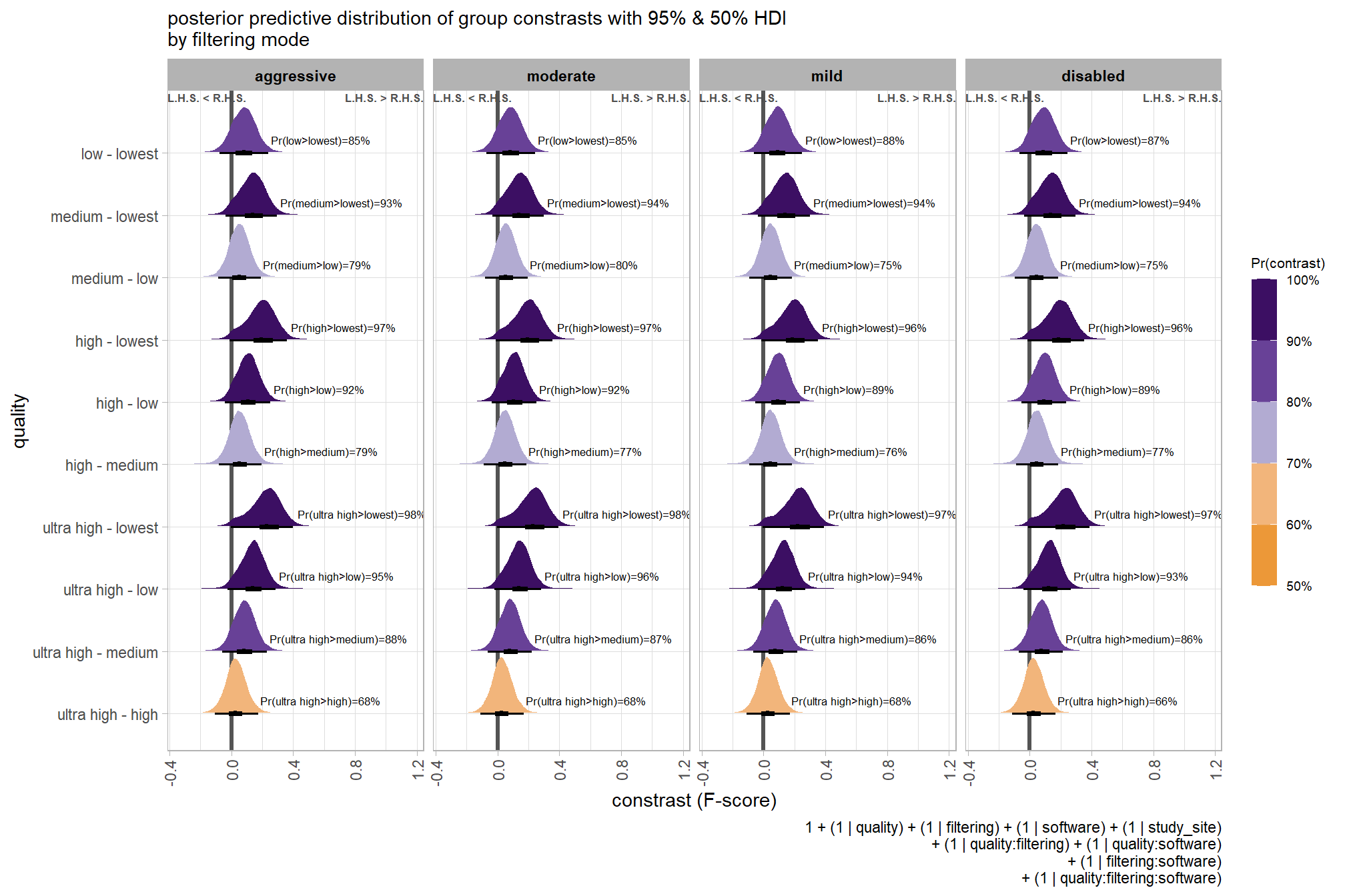
and summarize these contrasts
brms_contrast_temp %>%
  dplyr::group_by(contrast, depth_maps_generation_filtering_mode) %>%
  tidybayes::median_hdi(value) %>%
  dplyr::arrange(contrast, depth_maps_generation_filtering_mode) %>%
  dplyr::select(contrast, depth_maps_generation_filtering_mode, value, .lower, .upper) %>%

kableExtra::kbl(
    digits = 2
    , caption = "brms::brm model: 95% HDI of the posterior predictive distribution of group constrasts"
    , col.names = c(
      "quality contrast"
      , "filtering mode"
      , "difference (F-score)"
      , "HDI low", "HDI high"
    )
  ) %>%
  kableExtra::kable_styling() %>%
kableExtra::scroll_box(height = "8in")| quality contrast | filtering mode | difference (F-score) | HDI low | HDI high |
|---|---|---|---|---|
| ultra high - high | aggressive | 0.03 | -0.11 | 0.17 |
| ultra high - high | moderate | 0.03 | -0.11 | 0.17 |
| ultra high - high | mild | 0.03 | -0.11 | 0.17 |
| ultra high - high | disabled | 0.03 | -0.11 | 0.17 |
| ultra high - medium | aggressive | 0.08 | -0.06 | 0.23 |
| ultra high - medium | moderate | 0.08 | -0.06 | 0.22 |
| ultra high - medium | mild | 0.08 | -0.07 | 0.22 |
| ultra high - medium | disabled | 0.08 | -0.07 | 0.22 |
| ultra high - low | aggressive | 0.14 | -0.02 | 0.29 |
| ultra high - low | moderate | 0.14 | -0.02 | 0.28 |
| ultra high - low | mild | 0.13 | -0.04 | 0.27 |
| ultra high - low | disabled | 0.12 | -0.04 | 0.27 |
| ultra high - lowest | aggressive | 0.23 | 0.00 | 0.40 |
| ultra high - lowest | moderate | 0.23 | 0.00 | 0.39 |
| ultra high - lowest | mild | 0.22 | -0.01 | 0.39 |
| ultra high - lowest | disabled | 0.22 | -0.01 | 0.39 |
| high - medium | aggressive | 0.05 | -0.08 | 0.20 |
| high - medium | moderate | 0.05 | -0.09 | 0.19 |
| high - medium | mild | 0.05 | -0.09 | 0.18 |
| high - medium | disabled | 0.05 | -0.09 | 0.19 |
| high - low | aggressive | 0.11 | -0.04 | 0.25 |
| high - low | moderate | 0.11 | -0.04 | 0.25 |
| high - low | mild | 0.09 | -0.05 | 0.24 |
| high - low | disabled | 0.09 | -0.05 | 0.24 |
| high - lowest | aggressive | 0.20 | -0.01 | 0.36 |
| high - lowest | moderate | 0.20 | -0.01 | 0.36 |
| high - lowest | mild | 0.19 | -0.02 | 0.35 |
| high - lowest | disabled | 0.19 | -0.02 | 0.35 |
| medium - low | aggressive | 0.05 | -0.09 | 0.19 |
| medium - low | moderate | 0.06 | -0.08 | 0.20 |
| medium - low | mild | 0.05 | -0.09 | 0.18 |
| medium - low | disabled | 0.05 | -0.09 | 0.18 |
| medium - lowest | aggressive | 0.14 | -0.04 | 0.30 |
| medium - lowest | moderate | 0.14 | -0.03 | 0.30 |
| medium - lowest | mild | 0.14 | -0.04 | 0.30 |
| medium - lowest | disabled | 0.14 | -0.04 | 0.29 |
| low - lowest | aggressive | 0.08 | -0.08 | 0.24 |
| low - lowest | moderate | 0.08 | -0.07 | 0.24 |
| low - lowest | mild | 0.09 | -0.06 | 0.25 |
| low - lowest | disabled | 0.09 | -0.07 | 0.25 |
It might be more important to understand the difference in F-score by dense cloud quality and software rather than filtering mode since filtering mode had such a small effect on the SfM predictive ability
Note that how within tidybayes::add_epred_draws, we used the re_formula argument to average over the random effects of depth_maps_generation_filtering_mode. For this model we have to collapse across the filtering mode effects to compare the dense cloud quality and software setting effects.
ptcld_validation_data %>%
  dplyr::distinct(depth_maps_generation_quality, software) %>%
  tidybayes::add_epred_draws(
    brms_f_mod4, allow_new_levels = T
    # this part is crucial
    , re_formula = ~ (1 | depth_maps_generation_quality) +
      (1 | software) +
      (1 | depth_maps_generation_quality:software)
  ) %>%
  dplyr::rename(value = .epred) %>%
  dplyr::mutate(depth_maps_generation_quality = depth_maps_generation_quality %>% forcats::fct_rev()) %>%
  # plot
  ggplot(
    mapping = aes(
      y = value, x = software
      , fill = software
    )
  ) +
  tidybayes::stat_eye(
    point_interval = median_hdi, .width = .95
    , slab_alpha = 0.8
    , interval_color = "black", linewidth = 1
    , point_color = "black", point_fill = "black", point_size = 1
  ) +
  scale_fill_viridis_d(option = "rocket", begin = 0.3, end = 0.9, drop = F) +
  scale_y_continuous(breaks = scales::extended_breaks(n=10)) +
  facet_grid(cols = vars(depth_maps_generation_quality)) +
  labs(
    x = "software", y = "F-score"
    , subtitle = "posterior predictive distribution of F-score with 95% HDI\nby dense cloud quality"
    , caption = form_temp
  ) +
  theme_light() +
  theme(
    legend.position = "none"
    , legend.direction  = "horizontal"
    , axis.text.x = element_text(angle = 90, vjust = 0.5, hjust = 1)
    , strip.text = element_text(color = "black", face = "bold")
) 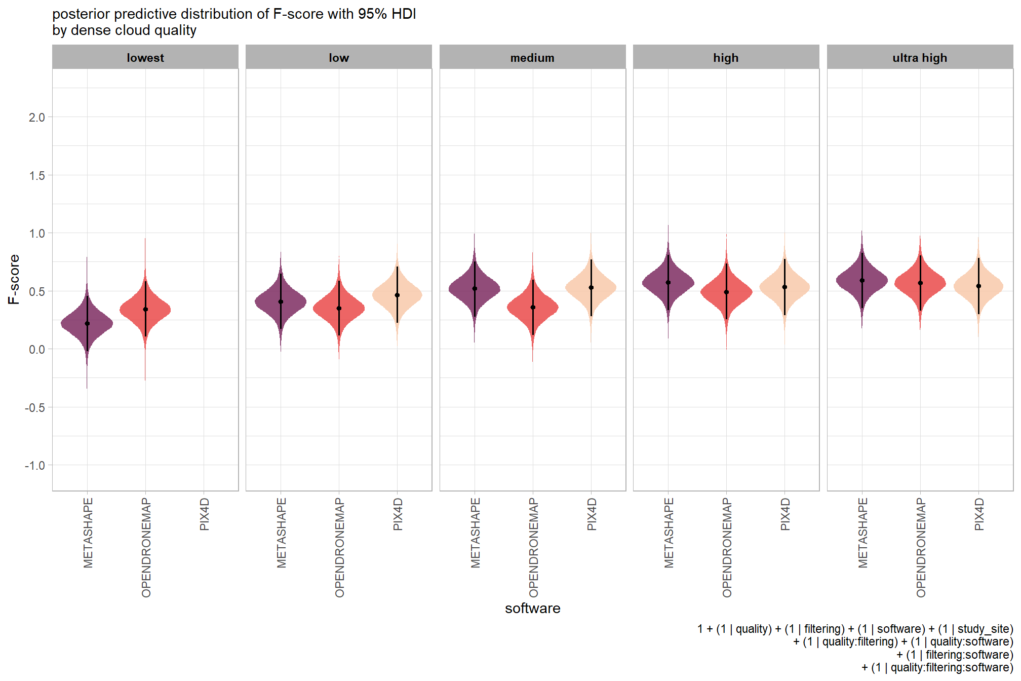
we can also make pairwise comparisons so long as we continue using tidybayes::add_epred_draws with the re_formula argument
# get draws
qlty_sftwr_draws_temp = ptcld_validation_data %>%
  dplyr::distinct(depth_maps_generation_quality, software) %>%
  tidybayes::add_epred_draws(
    brms_f_mod4, allow_new_levels = T
    # this part is crucial
    , re_formula = ~ (1 | depth_maps_generation_quality) +
      (1 | software) +
      (1 | depth_maps_generation_quality:software)
  ) %>%
  dplyr::rename(value = .epred)

# calculate contrast
brms_contrast_temp = qlty_sftwr_draws_temp %>%
  tidybayes::compare_levels(
    value
    , by = depth_maps_generation_quality
    , comparison =
      contrast_list[!stringr::str_detect(contrast_list, "lowest")]
      # contrast_list
  ) %>%
  dplyr::rename(contrast = depth_maps_generation_quality)

# separate contrast
brms_contrast_temp = brms_contrast_temp %>%
  dplyr::ungroup() %>%
  tidyr::separate_wider_delim(
    cols = contrast
    , delim = " - "
    , names = paste0(
      "sorter"
      , 1:(max(stringr::str_count(brms_contrast_temp$contrast, "-"))+1)
    )
    , too_few = "align_start"
    , cols_remove = F
  ) %>%
  dplyr::filter(sorter1!=sorter2) %>%
  dplyr::mutate(
    dplyr::across(
      tidyselect::starts_with("sorter")
      , .fns = function(x){factor(
        x, ordered = T
        , levels = levels(ptcld_validation_data$depth_maps_generation_quality)
      )}
    )
    , contrast = contrast %>%
      forcats::fct_reorder(
        paste0(as.numeric(sorter1), as.numeric(sorter2)) %>%
          as.numeric()
      )
  ) %>%
  # median_hdi summary for coloring
  dplyr::group_by(contrast, software) %>%
  make_contrast_vars()

# what?
brms_contrast_temp %>% dplyr::glimpse()
## Rows: 720,000
## Columns: 19
## Groups: contrast, software [18]
## $ software <chr> "METASHAPE", "METASHAPE", "METASHAPE", "METASHAPE", "…
## $ .chain <int> NA, NA, NA, NA, NA, NA, NA, NA, NA, NA, NA, NA, NA, N…
## $ .iteration <int> NA, NA, NA, NA, NA, NA, NA, NA, NA, NA, NA, NA, NA, N…
## $ .draw <int> 1, 2, 3, 4, 5, 6, 7, 8, 9, 10, 11, 12, 13, 14, 15, 16…
## $ sorter1 <ord> ultra high, ultra high, ultra high, ultra high, ultra…
## $ sorter2 <ord> high, high, high, high, high, high, high, high, high,…
## $ contrast <fct> ultra high - high, ultra high - high, ultra high - hi…
## $ value <dbl> 0.011002873, 0.016403992, 0.036585434, -0.007965928, …
## $ median_hdi_est <dbl> 0.01895816, 0.01895816, 0.01895816, 0.01895816, 0.018…
## $ median_hdi_lower <dbl> -0.07011604, -0.07011604, -0.07011604, -0.07011604, -…
## $ median_hdi_upper <dbl> 0.1084027, 0.1084027, 0.1084027, 0.1084027, 0.1084027…
## $ pr_gt_zero <chr> "66%", "66%", "66%", "66%", "66%", "66%", "66%", "66%…
## $ pr_lt_zero <chr> "34%", "34%", "34%", "34%", "34%", "34%", "34%", "34%…
## $ is_diff_dir <lgl> TRUE, TRUE, TRUE, FALSE, FALSE, TRUE, FALSE, TRUE, TR…
## $ pr_diff <dbl> 0.662975, 0.662975, 0.662975, 0.662975, 0.662975, 0.6…
## $ pr_diff_lab <chr> "Pr(ultra high>high)=66%", "Pr(ultra high>high)=66%",…
## $ pr_diff_lab_sm <chr> "Pr(>0)=66%", "Pr(>0)=66%", "Pr(>0)=66%", "Pr(>0)=66%…
## $ pr_diff_lab_pos <dbl> 0.1165329, 0.1165329, 0.1165329, 0.1165329, 0.1165329…
## $ sig_level <ord> <80%, <80%, <80%, <80%, <80%, <80%, <80%, <80%, <80%,…plot it
plt_contrast(
  brms_contrast_temp, caption_text = form_temp
  , y_axis_title = "quality"
  , facet = "software"
  , label_size = 2.1
  , x_expand = c(0,0.5)
) +
  labs(
    subtitle = "posterior predictive distribution of group constrasts with 95% & 50% HDI\nby software"
  )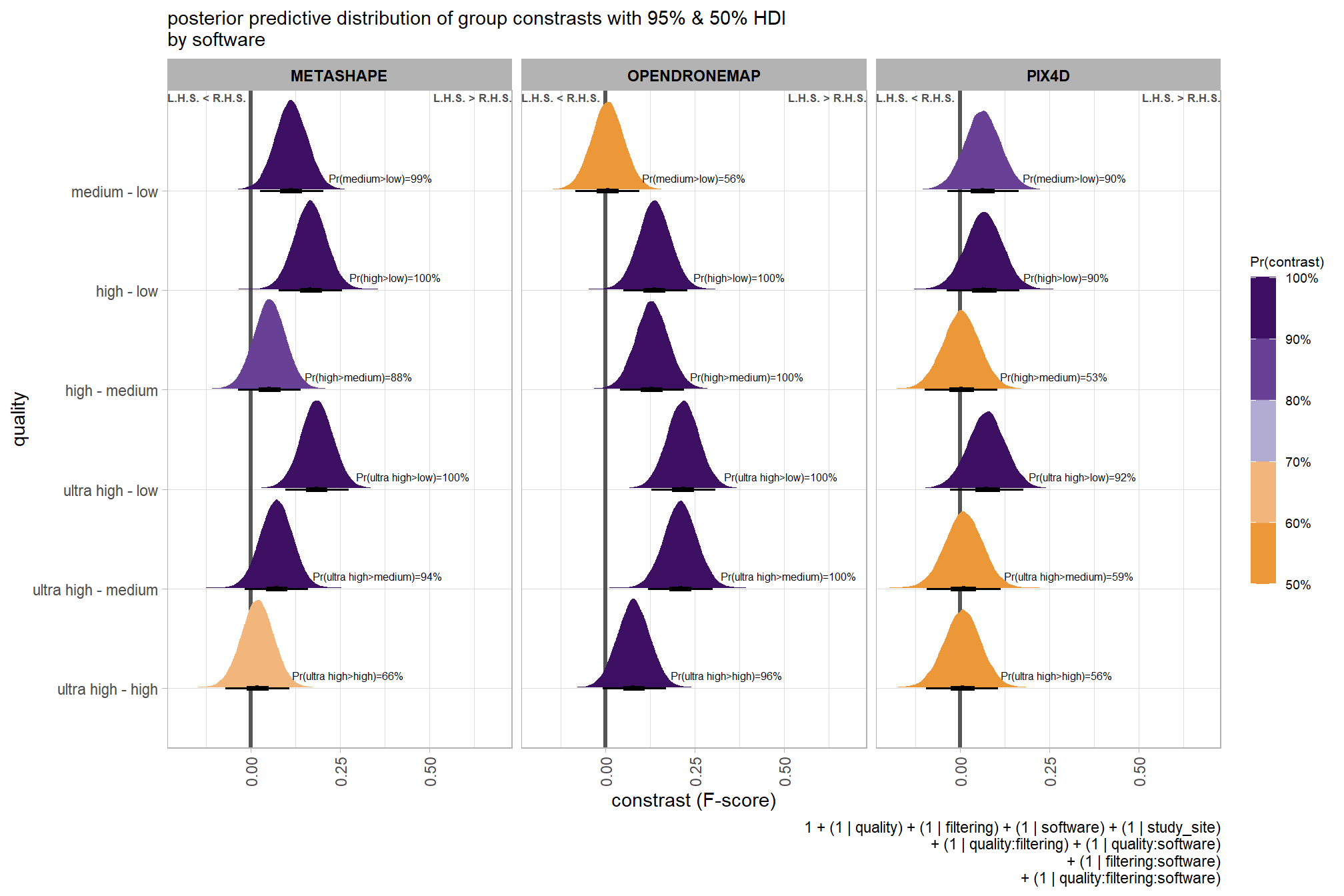
ggplot2::ggsave(
  "../data/qlty_sftwr_comp_mod4.png"
  , plot = ggplot2::last_plot() + labs(subtitle = "")
  , height = 7, width = 10.5
)
and summarize these contrasts
brms_contrast_temp %>%
  dplyr::group_by(contrast, software) %>%
  tidybayes::median_hdi(value) %>%
  dplyr::arrange(contrast, software) %>%
  dplyr::select(contrast, software, value, .lower, .upper) %>%

  kableExtra::kbl(
    digits = 2
    , caption = "brms::brm model: 95% HDI of the posterior predictive distribution of group constrasts"
    , col.names = c(
      "quality contrast"
      , "software"
      , "difference (F-score)"
      , "HDI low", "HDI high"
    )
  ) %>%
  kableExtra::kable_styling() %>%
kableExtra::scroll_box(height = "6in")| quality contrast | software | difference (F-score) | HDI low | HDI high |
|---|---|---|---|---|
| ultra high - high | METASHAPE | 0.02 | -0.07 | 0.11 |
| ultra high - high | OPENDRONEMAP | 0.08 | -0.01 | 0.17 |
| ultra high - high | PIX4D | 0.01 | -0.09 | 0.11 |
| ultra high - medium | METASHAPE | 0.07 | -0.02 | 0.16 |
| ultra high - medium | OPENDRONEMAP | 0.21 | 0.12 | 0.30 |
| ultra high - medium | PIX4D | 0.01 | -0.09 | 0.11 |
| ultra high - low | METASHAPE | 0.19 | 0.10 | 0.27 |
| ultra high - low | OPENDRONEMAP | 0.22 | 0.13 | 0.31 |
| ultra high - low | PIX4D | 0.08 | -0.03 | 0.18 |
| high - medium | METASHAPE | 0.05 | -0.03 | 0.14 |
| high - medium | OPENDRONEMAP | 0.13 | 0.04 | 0.22 |
| high - medium | PIX4D | 0.00 | -0.10 | 0.10 |
| high - low | METASHAPE | 0.17 | 0.08 | 0.26 |
| high - low | OPENDRONEMAP | 0.14 | 0.05 | 0.23 |
| high - low | PIX4D | 0.07 | -0.04 | 0.17 |
| medium - low | METASHAPE | 0.11 | 0.03 | 0.20 |
| medium - low | OPENDRONEMAP | 0.01 | -0.08 | 0.10 |
| medium - low | PIX4D | 0.06 | -0.04 | 0.16 |
The contrasts above address the question “are there differences in F-score based on dense point cloud generation quality within each software?”.
To address the different question of “are there differences in F-score based on the processing software used at a given dense point cloud generation quality?” we need to utilize a different formulation of the comparison parameter within our call to the tidybayes::compare_levels function and calculate the contrast by software instead
# calculate contrast
brms_contrast_temp = qlty_sftwr_draws_temp %>%
  tidybayes::compare_levels(
    value
    , by = software
    , comparison = "pairwise"
  ) %>%
  dplyr::rename(contrast = software) %>%
  # median_hdi summary for coloring
  dplyr::group_by(contrast, depth_maps_generation_quality) %>%
  make_contrast_vars()

# what?
brms_contrast_temp %>% dplyr::glimpse()
## Rows: 520,000
## Columns: 17
## Groups: contrast, depth_maps_generation_quality [13]
## $ depth_maps_generation_quality <ord> ultra high, ultra high, ultra high, ultr…
## $ .chain <int> NA, NA, NA, NA, NA, NA, NA, NA, NA, NA, …
## $ .iteration <int> NA, NA, NA, NA, NA, NA, NA, NA, NA, NA, …
## $ .draw <int> 1, 2, 3, 4, 5, 6, 7, 8, 9, 10, 11, 12, 1…
## $ contrast <chr> "OPENDRONEMAP - METASHAPE", "OPENDRONEMA…
## $ value <dbl> -0.041567216, -0.044398847, 0.038336862,…
## $ median_hdi_est <dbl> -0.02216649, -0.02216649, -0.02216649, -…
## $ median_hdi_lower <dbl> -0.1270756, -0.1270756, -0.1270756, -0.1…
## $ median_hdi_upper <dbl> 0.0801044, 0.0801044, 0.0801044, 0.08010…
## $ pr_gt_zero <chr> "33%", "33%", "33%", "33%", "33%", "33%"…
## $ pr_lt_zero <chr> "67%", "67%", "67%", "67%", "67%", "67%"…
## $ is_diff_dir <lgl> TRUE, TRUE, FALSE, TRUE, TRUE, TRUE, TRU…
## $ pr_diff <dbl> 0.6705, 0.6705, 0.6705, 0.6705, 0.6705, …
## $ pr_diff_lab <chr> "Pr(MtaShp>ODM)=67%", "Pr(MtaShp>ODM)=67…
## $ pr_diff_lab_sm <chr> "Pr(<0)=67%", "Pr(<0)=67%", "Pr(<0)=67%"…
## $ pr_diff_lab_pos <dbl> -0.1366063, -0.1366063, -0.1366063, -0.1…
## $ sig_level <ord> <80%, <80%, <80%, <80%, <80%, <80%, <80%…plot it
plt_contrast(
  brms_contrast_temp, caption_text = form_temp
  , y_axis_title = "software"
  , facet = "depth_maps_generation_quality"
  , label_size = 2.0
  , x_expand = c(0.3,0.3)
) +
  facet_wrap(facets = vars(depth_maps_generation_quality), ncol = 2) +
  labs(
    subtitle = "posterior predictive distribution of group constrasts with 95% & 50% HDI\nby dense cloud quality"
  ) +
  theme(
    legend.position = c(.75, .13)
  ) +
  guides(fill = guide_colorbar(theme = theme(
    legend.key.width  = unit(1, "lines"),
    legend.key.height = unit(7, "lines")
  )))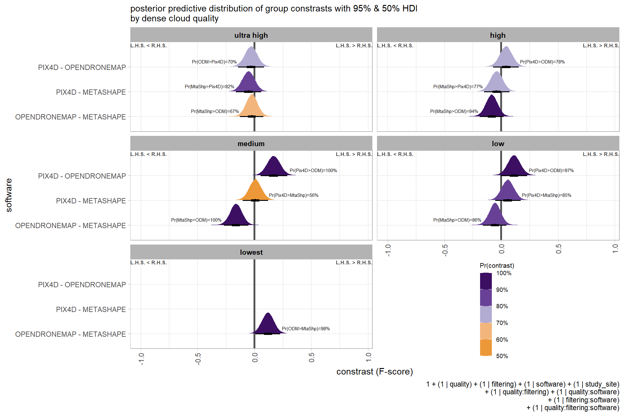
and summarize these contrasts
brms_contrast_temp %>%
  dplyr::group_by(contrast, depth_maps_generation_quality) %>%
  tidybayes::median_hdi(value) %>%
  dplyr::arrange(contrast, depth_maps_generation_quality) %>%
  dplyr::select(contrast, depth_maps_generation_quality, value, .lower, .upper) %>%

  kableExtra::kbl(
    digits = 2
    , caption = "brms::brm model: 95% HDI of the posterior predictive distribution of group constrasts"
    , col.names = c(
      "software contrast"
      , "quality"
      , "difference (F-score)"
      , "HDI low", "HDI high"
    )
  ) %>%
  kableExtra::kable_styling() %>%
kableExtra::scroll_box(height = "8in")| software contrast | quality | difference (F-score) | HDI low | HDI high |
|---|---|---|---|---|
| OPENDRONEMAP - METASHAPE | ultra high | -0.02 | -0.13 | 0.08 |
| OPENDRONEMAP - METASHAPE | high | -0.08 | -0.19 | 0.02 |
| OPENDRONEMAP - METASHAPE | medium | -0.16 | -0.27 | -0.05 |
| OPENDRONEMAP - METASHAPE | low | -0.05 | -0.16 | 0.05 |
| OPENDRONEMAP - METASHAPE | lowest | 0.12 | 0.01 | 0.23 |
| PIX4D - METASHAPE | ultra high | -0.05 | -0.16 | 0.06 |
| PIX4D - METASHAPE | high | -0.04 | -0.15 | 0.07 |
| PIX4D - METASHAPE | medium | 0.01 | -0.10 | 0.12 |
| PIX4D - METASHAPE | low | 0.06 | -0.05 | 0.17 |
| PIX4D - OPENDRONEMAP | ultra high | -0.03 | -0.14 | 0.08 |
| PIX4D - OPENDRONEMAP | high | 0.04 | -0.07 | 0.15 |
| PIX4D - OPENDRONEMAP | medium | 0.17 | 0.06 | 0.29 |
| PIX4D - OPENDRONEMAP | low | 0.11 | 0.00 | 0.23 |
let’s collapse across the filtering mode, software, and study site to compare the dense cloud quality setting effect.
In a hierarchical model structure, we have to make use of the re_formula argument within tidybayes::add_epred_draws
ptcld_validation_data %>%
  dplyr::distinct(depth_maps_generation_quality) %>%
  tidybayes::add_epred_draws(
    brms_f_mod4
    # this part is crucial
    , re_formula = ~ (1 | depth_maps_generation_quality)
  ) %>%
  dplyr::rename(value = .epred) %>%
  # plot
  ggplot(
    mapping = aes(
      x = value, y = depth_maps_generation_quality
      , fill = depth_maps_generation_quality
    )
  ) +
    tidybayes::stat_halfeye(
      point_interval = median_hdi, .width = .95
      , interval_color = "gray66"
      , shape = 21, point_color = "gray66", point_fill = "black"
      , justification = -0.01
    ) +
    scale_fill_viridis_d(option = "inferno", drop = F) +
    scale_x_continuous(breaks = scales::extended_breaks(n=8)) +
    labs(
      y = "quality", x = "F-score"
      , subtitle = "posterior predictive distribution of F-score with 95% HDI"
      , caption = form_temp
    ) +
    theme_light() +
    theme(legend.position = "none")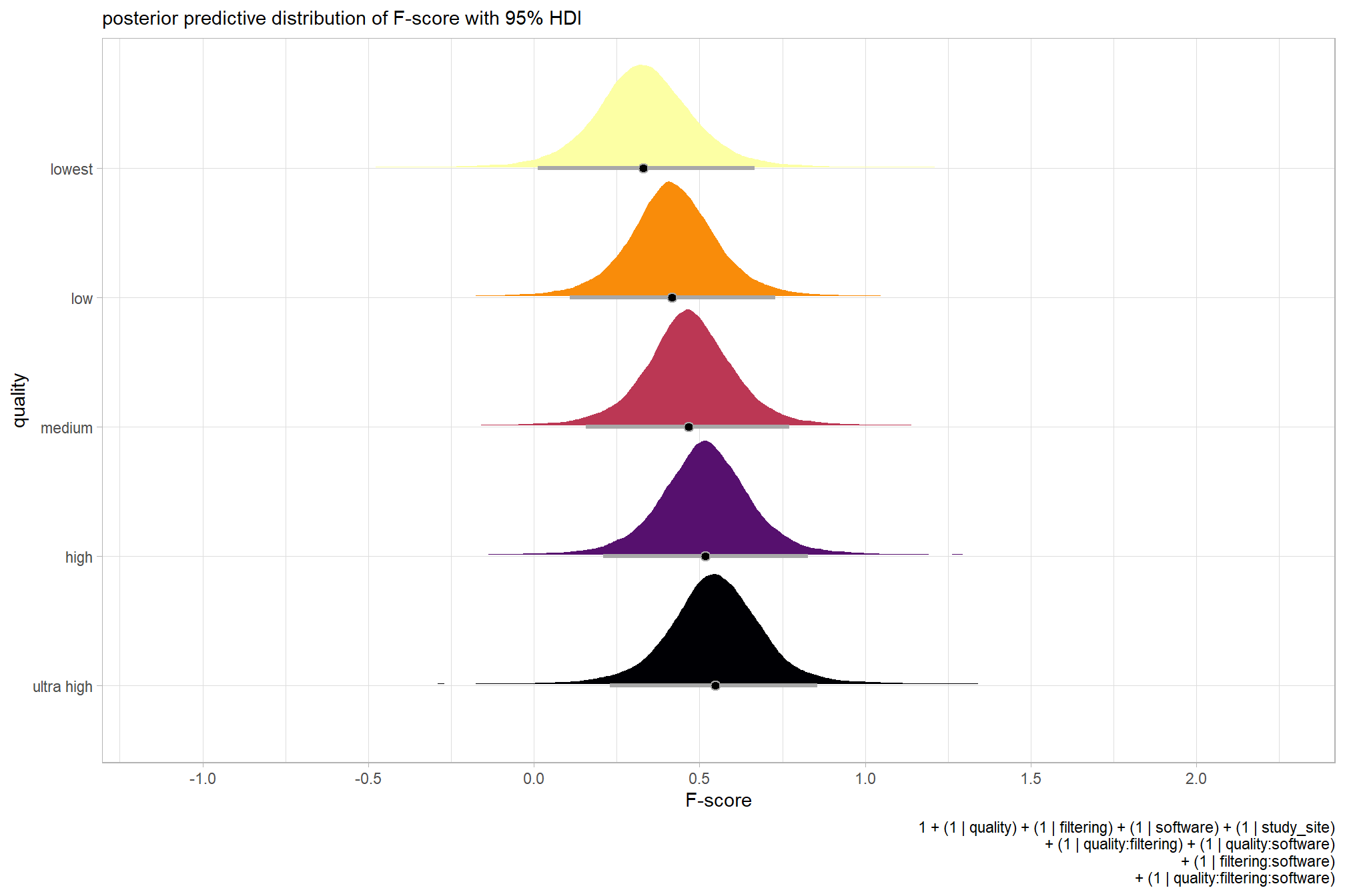
let’s compare these results to the results from our one nominal predictor model above, two nominal predictor model above, and three nominal predictor model above
ptcld_validation_data %>%
  dplyr::distinct(depth_maps_generation_quality) %>%
  tidybayes::add_epred_draws(
    brms_f_mod4
    # this part is crucial
    , re_formula = ~ (1 | depth_maps_generation_quality)
  ) %>%
  dplyr::mutate(value = .epred, src = "brms_f_mod4") %>%
  dplyr::bind_rows(
    ptcld_validation_data %>%
      dplyr::distinct(depth_maps_generation_quality) %>%
      tidybayes::add_epred_draws(
        brms_f_mod3
        # this part is crucial
        , re_formula = ~ (1 | depth_maps_generation_quality)
      ) %>%
      dplyr::mutate(value = .epred, src = "brms_f_mod3")
    , ptcld_validation_data %>%
      dplyr::distinct(depth_maps_generation_quality) %>%
      tidybayes::add_epred_draws(
        brms_f_mod2
        # this part is crucial
        , re_formula = ~ (1 | depth_maps_generation_quality)
      ) %>%
      dplyr::mutate(value = .epred, src = "brms_f_mod2")
    , ptcld_validation_data %>%
      dplyr::distinct(depth_maps_generation_quality) %>%
      tidybayes::add_epred_draws(brms_f_mod1) %>%
      dplyr::mutate(value = .epred, src = "brms_f_mod1")
  ) %>%
  ggplot(mapping = aes(y = src, x = value, color = src, group = src)) +
  tidybayes::stat_pointinterval(position = "dodge") +
  facet_grid(rows = vars(depth_maps_generation_quality), switch = "y") +
  scale_y_discrete(NULL, breaks = NULL) +
  scale_color_manual(values = viridis::turbo(n = 6, begin = 0.2, end = 0.8)[1:4]) +
  labs(
    y = "", x = "F-score"
    , color = "model"
  ) +
  theme_light() +
  theme(legend.position = "top", strip.text = element_text(color = "black", face = "bold"))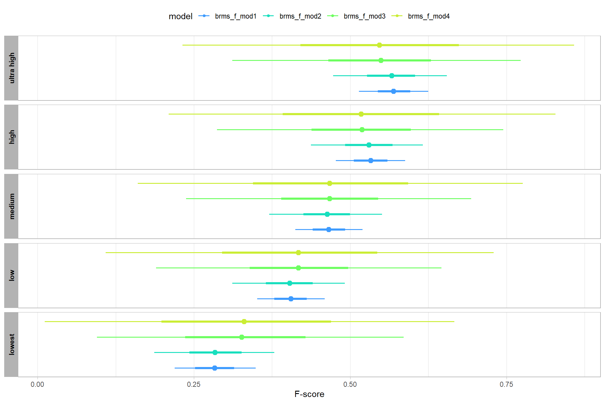
let’s also collapse across the dense cloud quality, software, and study site to compare the filtering mode setting effect.
In a hierarchical model structure, we have to make use of the re_formula argument within tidybayes::add_epred_draws
ptcld_validation_data %>%
  dplyr::distinct(depth_maps_generation_filtering_mode) %>%
  tidybayes::add_epred_draws(
    brms_f_mod4
    # this part is crucial
    , re_formula = ~ (1 | depth_maps_generation_filtering_mode)
  ) %>%
  dplyr::rename(value = .epred) %>%
  # plot
  ggplot(
    mapping = aes(
      x = value, y = depth_maps_generation_filtering_mode
      , fill = depth_maps_generation_filtering_mode
    )
  ) +
    tidybayes::stat_halfeye(
      point_interval = median_hdi, .width = .95
      , interval_color = "gray66"
      , shape = 21, point_color = "gray66", point_fill = "black"
      , justification = -0.01
    ) +
    scale_fill_viridis_d(option = "plasma", drop = F) +
    scale_x_continuous(breaks = scales::extended_breaks(n=8)) +
    labs(
      y = "filtering mode", x = "F-score"
      , subtitle = "posterior predictive distribution of F-score with 95% HDI"
      , caption = form_temp
    ) +
    theme_light() +
    theme(legend.position = "none")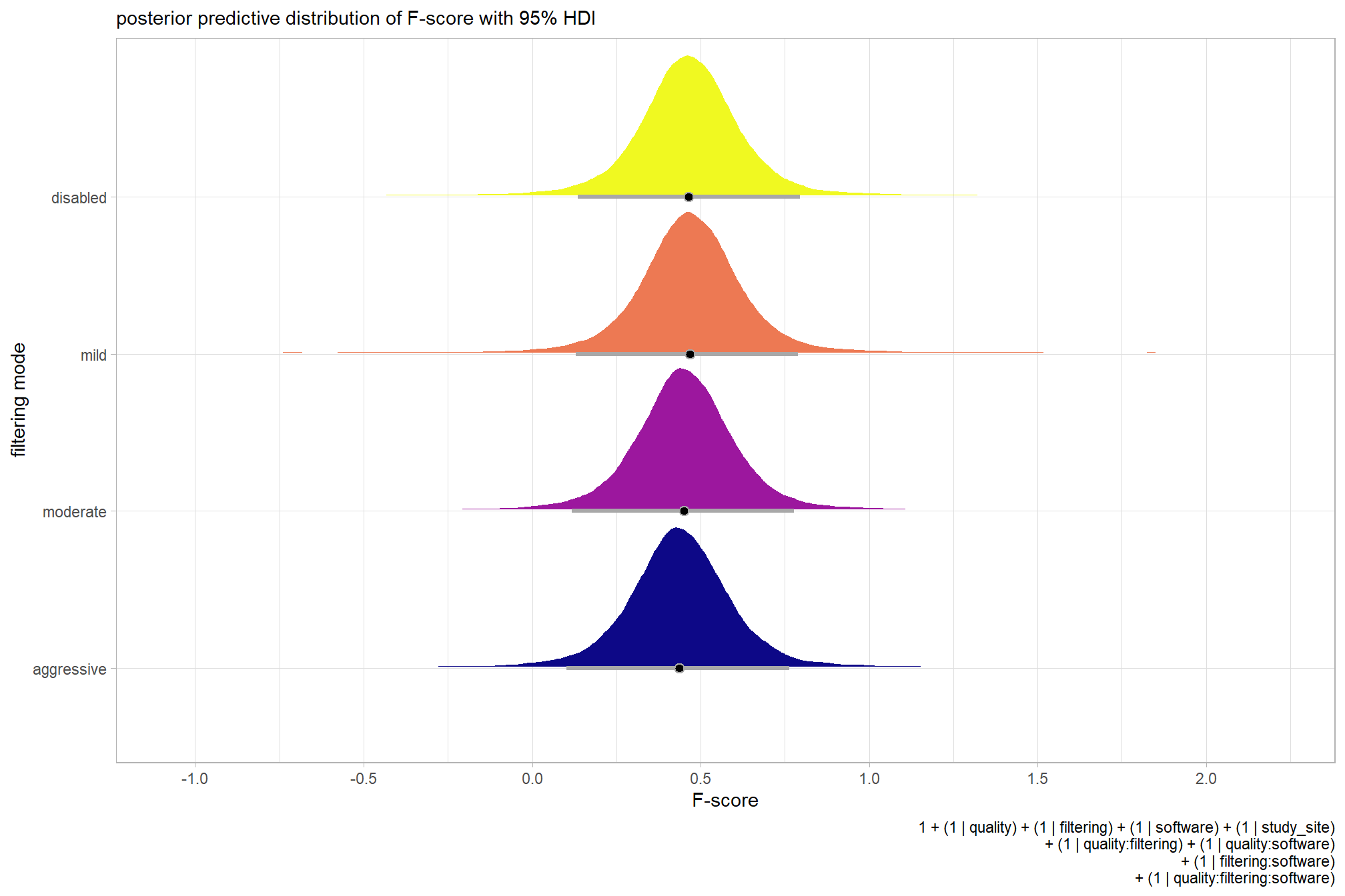
let’s compare these results to the results from two nominal predictor model above and three nominal predictor model above
ptcld_validation_data %>%
  dplyr::distinct(depth_maps_generation_filtering_mode) %>%
  tidybayes::add_epred_draws(
    brms_f_mod4
    # this part is crucial
    , re_formula = ~ (1 | depth_maps_generation_filtering_mode)
  ) %>%
  dplyr::mutate(value = .epred, src = "brms_f_mod4") %>%
  dplyr::bind_rows(
    ptcld_validation_data %>%
      dplyr::distinct(depth_maps_generation_filtering_mode) %>%
      tidybayes::add_epred_draws(
        brms_f_mod3
        # this part is crucial
        , re_formula = ~ (1 | depth_maps_generation_filtering_mode)
      ) %>%
      dplyr::mutate(value = .epred, src = "brms_f_mod3")
    , ptcld_validation_data %>%
      dplyr::distinct(depth_maps_generation_filtering_mode) %>%
      tidybayes::add_epred_draws(
        brms_f_mod2
        # this part is crucial
        , re_formula = ~ (1 | depth_maps_generation_filtering_mode)
      ) %>%
      dplyr::mutate(value = .epred, src = "brms_f_mod2")
  ) %>%
  ggplot(mapping = aes(y = src, x = value, color = src, group = src)) +
  tidybayes::stat_pointinterval(position = "dodge") +
  facet_grid(rows = vars(depth_maps_generation_filtering_mode), switch = "y") +
  scale_y_discrete(NULL, breaks = NULL) +
  scale_color_manual(values = viridis::turbo(n = 6, begin = 0.2, end = 0.8)[2:4]) +
  labs(
    y = "filtering mode", x = "F-score"
    , color = "model"
  ) +
  theme_light() +
  theme(legend.position = "top", strip.text = element_text(color = "black", face = "bold"))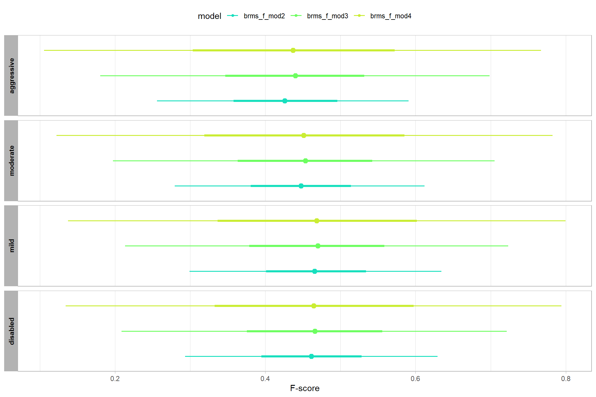
to address one of our main questions, let’s also collapse across the study site, dense cloud quality, and filtering mode setting to compare the software effect.
In a hierarchical model structure, we have to make use of the re_formula argument within tidybayes::add_epred_draws
ptcld_validation_data %>%
  dplyr::distinct(software) %>%
  tidybayes::add_epred_draws(
    brms_f_mod4
    # this part is crucial
    , re_formula = ~ (1 | software)
  ) %>%
  dplyr::rename(value = .epred) %>%
  # plot
  ggplot(
    mapping = aes(
      x = value, y = software
      , fill = software
    )
  ) +
    tidybayes::stat_halfeye(
      point_interval = median_hdi, .width = .95
      , interval_color = "gray66"
      , shape = 21, point_color = "gray66", point_fill = "black"
      , justification = -0.01
    ) +
    scale_fill_viridis_d(option = "rocket", begin = 0.3, end = 0.9, drop = F) +
    scale_x_continuous(breaks = scales::extended_breaks(n=8)) +
    labs(
      y = "software", x = "F-score"
      , subtitle = "posterior predictive distribution of F-score with 95% HDI"
      , caption = form_temp
    ) +
    theme_light() +
    theme(legend.position = "none")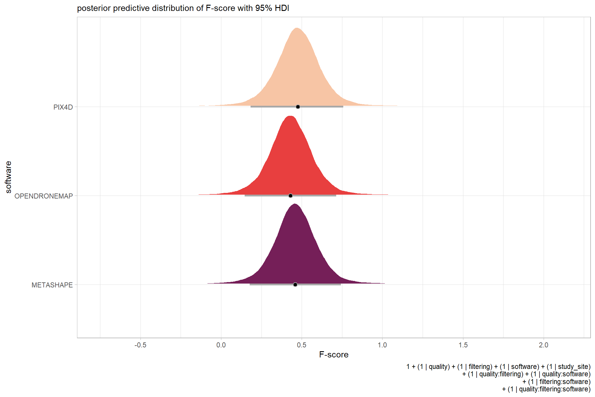
let’s compare these results to the results from our three nominal predictor model above
ptcld_validation_data %>%
  dplyr::distinct(software) %>%
  tidybayes::add_epred_draws(
    brms_f_mod4
    # this part is crucial
    , re_formula = ~ (1 | software)
  ) %>%
  dplyr::mutate(value = .epred, src = "brms_f_mod4") %>%
  dplyr::bind_rows(
    ptcld_validation_data %>%
      dplyr::distinct(software) %>%
      tidybayes::add_epred_draws(
        brms_f_mod3
        # this part is crucial
        , re_formula = ~ (1 | software)
      ) %>%
      dplyr::mutate(value = .epred, src = "brms_f_mod3")
  ) %>%
  ggplot(mapping = aes(y = src, x = value, color = src, group = src)) +
  tidybayes::stat_pointinterval(position = "dodge") +
  facet_grid(rows = vars(software), switch = "y") +
  scale_y_discrete(NULL, breaks = NULL) +
  scale_color_manual(values = viridis::turbo(n = 6, begin = 0.2, end = 0.8)[3:4]) +
  labs(
    y = "", x = "F-score"
    , color = "model"
  ) +
  theme_light() +
  theme(legend.position = "top", strip.text = element_text(color = "black", face = "bold"))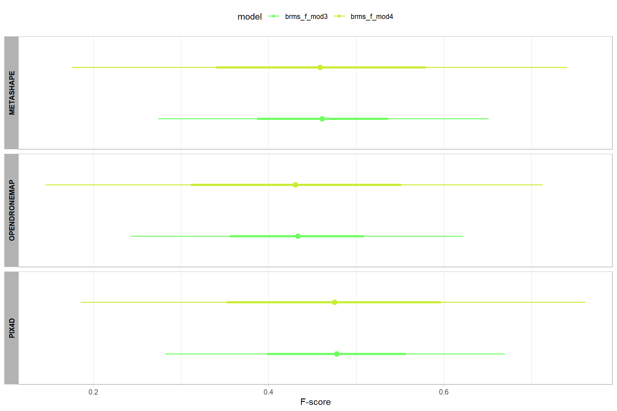
Finally, we can quantify the variation in F-score by comparing the \(\sigma\) posteriors.
# extract the posterior draws
brms::as_draws_df(brms_f_mod4) %>%
  dplyr::select(c(sigma,tidyselect::starts_with("sd_"))) %>%
  tidyr::pivot_longer(dplyr::everything()) %>%
  # dplyr::group_by(name) %>%
  # tidybayes::median_hdi(value) %>%
  dplyr::mutate(
    name = name %>%
      stringr::str_replace_all("depth_maps_generation_quality", "quality") %>%
      stringr::str_replace_all("depth_maps_generation_filtering_mode", "filtering") %>%
      forcats::fct_reorder(value)
  ) %>%
# plot
  ggplot(aes(x = value, y = name)) +
  tidybayes::stat_dotsinterval(
    point_interval = median_hdi, .width = .95
    , justification = -0.04
    , shape = 21 #, point_size = 3
    , quantiles = 100
  ) +
  labs(x = "", y = "", caption = form_temp) +
  theme_light()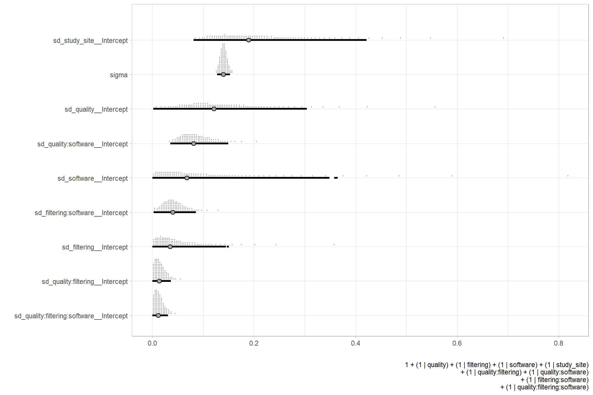
and perform model selection via information criteria with the brms::loo_compare() function
brms_f_mod4 = brms::add_criterion(brms_f_mod4, criterion = c("loo", "waic"))
brms::loo_compare(brms_f_mod1, brms_f_mod2, brms_f_mod3, brms_f_mod4, criterion = "loo")
## elpd_diff se_diff
## brms_f_mod4 0.0 0.0
## brms_f_mod3 -91.0 11.6
## brms_f_mod1 -91.3 11.0
## brms_f_mod2 -93.0 11.06.7 The beta: Three Nominal Predictors + site effects
To this point, we have been modelling F-score presuming a Gaussian likelihood. However, the beta likelihood more accurately represents the F-score data which is continuous and restricted within the range of \((0,1)\).
We borrow here from the excellent series on causal inference by A. Solomon Kurz. We also utilize the guide to Bayesian beta models by Andrew Heiss while Nicole Knight posted about the Beta for ecological data.
6.7.1 Summary Statistics
let’s check our underlying data for F-score (our dependent or \(y\) variable)
# distribution
ptcld_validation_data %>%
  ggplot(mapping = aes(x = f_score)) +
  geom_hline(yintercept = 0) +
  geom_vline(xintercept = c(0,1)) +
  geom_density(fill = "lightblue", alpha = 0.7, color = NA) +
  labs(y="",x="F-score") +
  scale_y_continuous(breaks = c(0)) +
  scale_x_continuous(breaks = scales::extended_breaks(10)) +
  theme_light() +
  theme(panel.grid = element_blank())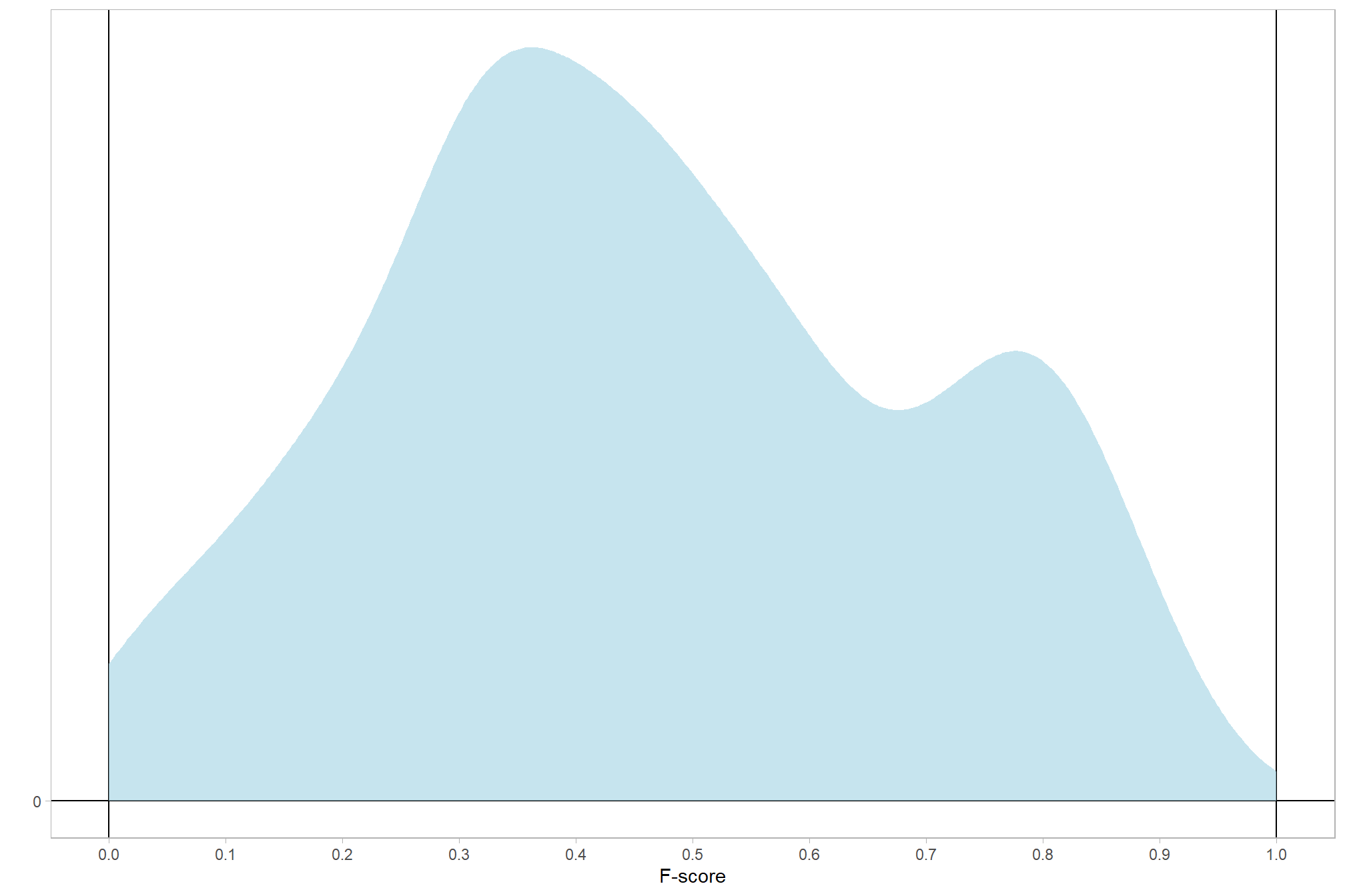
and the summary statistics
ptcld_validation_data %>%
  dplyr::ungroup() %>%
  dplyr::select(f_score) %>%
  dplyr::summarise(
    dplyr::across(
      dplyr::everything()
      , .fns = list(
        mean = ~ mean(.x,na.rm=T), median = ~ median(.x,na.rm=T), sd = ~ sd(.x,na.rm=T)
        , min = ~ min(.x,na.rm=T), max = ~ max(.x,na.rm=T)
        , q25 = ~ quantile(.x, 0.25, na.rm = T)
        , q75 = ~ quantile(.x, 0.75, na.rm = T)
      )
      , .names = "{.fn}"
    )
  ) %>%
  tidyr::pivot_longer(everything()) %>%
  kableExtra::kbl(caption = "summary: `f_score`", digits = 3, col.names = NULL) %>%
kableExtra::kable_styling()| mean | 0.461 |
| median | 0.442 |
| sd | 0.229 |
| min | 0.000 |
| max | 0.900 |
| q25 | 0.298 |
| q75 | 0.622 |
6.7.2 Bayesian
With the beta likelihood our model with three nominal predictor variables and subject-level effects the model becomes:
\[\begin{align*} y_{i} \sim & \operatorname{Beta} \bigl(\mu_{i}, \phi \bigr) \\ \operatorname{logit}(\mu_{i}) = & \beta_0 \\ & + \sum_{j=1}^{J=5} \beta_{1[j]} x_{1[j]} + \sum_{k=1}^{K=4} \beta_{2[k]} x_{2[k]} + \sum_{f=1}^{F=3} \beta_{3[f]} x_{3[f]} + \sum_{s=1}^{S=5} \beta_{4[s]} x_{4[s]} \\ & + \sum_{j,k} \beta_{1\times2[j,k]} x_{1\times2[j,k]} + \sum_{j,f} \beta_{1\times3[j,f]} x_{1\times3[j,f]} + \sum_{k,f} \beta_{2\times3[k,f]} x_{2\times3[k,f]} \\ & + \sum_{j,k,f} \beta_{1\times2\times3[j,k,f]} x_{1\times2\times3[j,k,f]} \\ \beta_{0} \sim & \operatorname{Normal}(0,1) \\ \beta_{1[j]} \sim & \operatorname{Normal}(0,\sigma_{\beta_{1}}) \\ \beta_{2[k]} \sim & \operatorname{Normal}(0,\sigma_{\beta_{2}}) \\ \beta_{3[f]} \sim & \operatorname{Normal}(0,\sigma_{\beta_{3}}) \\ \beta_{4[s]} \sim & \operatorname{Normal}(0,\sigma_{\beta_{4}}) \\ \beta_{1\times2[j,k]} \sim & \operatorname{Normal}(0,\sigma_{\beta_{1\times2}}) \\ \beta_{1\times3[j,f]} \sim & \operatorname{Normal}(0,\sigma_{\beta_{1\times3}}) \\ \beta_{2\times3[k,f]} \sim & \operatorname{Normal}(0,\sigma_{\beta_{2\times3}}) \\ \sigma_{\beta_{1}} \sim & \operatorname{Student T}(3,0,2.5) \\ \sigma_{\beta_{2}} \sim & \operatorname{Student T}(3,0,2.5) \\ \sigma_{\beta_{3}} \sim & \operatorname{Student T}(3,0,2.5) \\ \sigma_{\beta_{4}} \sim & \operatorname{Student T}(3,0,2.5) \\ \sigma_{\beta_{1\times2}} \sim & \operatorname{Student T}(3,0,2.5) \\ \sigma_{\beta_{1\times3}} \sim & \operatorname{Student T}(3,0,2.5) \\ \sigma_{\beta_{2\times3}} \sim & \operatorname{Student T}(3,0,2.5) \\ \phi \sim & \operatorname{Gamma}(0.1,0.1) \\ \end{align*}\]
, where \(j\) is the depth map generation quality setting corresponding to observation \(i\), \(k\) is the depth map filtering mode setting corresponding to observation \(i\), \(f\) is the processing software corresponding to observation \(i\), and \(s\) is the study site corresponding to observation \(i\)
Per brms, our \(y\) is \(\operatorname{Beta}\) distributed with the mean as \(\mu\) and the concentration as \(\phi\) which is sometimes called the concentration, sample size or precision. We can think of mean (\(\mu\)) and precision (\(\phi\)) just like with a normal distribution and its mean and standard deviation.
brms allows us to model the precision (\(\phi\)) but it is not required. If \(\phi\) is not modeled, you still get a precision component, but it is universal across all the different coefficients (it doesn’t vary across any variables in the model). Heiss explains that:
for whatever mathy reasons, when you don’t explicitly model the precision, the resulting coefficient in the table isn’t on the log scale—it’s a regular non-logged number, so there’s no need to exponentiate.
in thie brms community post it is similarly noted that:
If you don’t predict the parameters, you give priors for them on non-transformed scale. When you predict them, the predictors become linear coefficients as any other and work on the transformed scale - the transformations are specified by the link_XX parameters of the families (and you can change them if you need).
6.7.2.1 Prior distributions
#### setting priors
# required libraries: tidyverse, tidybayes, brms, palettetown, latex2exp
brms_f_mod5_priors_temp <- c(
    brms::prior(normal(0, 1), class = "Intercept")
    , brms::prior(student_t(3, 0, 2.5), class = "sd")
    , brms::prior(gamma(0.1, 0.1), class = phi)
  )
# plot
brms_f_mod5_priors_temp %>%
  tidybayes::parse_dist() %>%
  tidybayes::marginalize_lkjcorr(K = 2) %>%
  mutate(
    distrib = case_when(
      prior == "student_t(3, 0, 2.5)" ~ latex2exp::TeX(r'($\sigma \sim Student\,T(3, 0, 2.5)$)', output = "character"),
      prior == "normal(0, 1)" ~ latex2exp::TeX(r'($\beta \sim Normal(0, 1)$)',  output = "character"),
      prior == "gamma(0.1, 0.1)" ~ latex2exp::TeX(r'($\phi \sim$ Gamma(0.1, 0.1))',  output = "character")
  )) %>%
  ggplot(., aes(dist = .dist, args = .args)) +
  facet_wrap(vars(distrib), scales = "free", labeller = label_parsed) +
  ggdist::stat_halfeye(
    aes(fill = prior),
    n = 10e2,
    show.legend = F
    , fill = "slategray"
  ) +
  coord_flip() +
  theme_light() +
  theme(
    strip.text = element_text(face = "bold", color = "black"),
    axis.text.y = element_blank(),
    axis.ticks = element_blank()
    , plot.subtitle = element_text(size = 8)
    , plot.title = element_text(size = 9)
  )+
  labs(
    x = "",
    title = "Priors: F-Score",
    y = "Log Odds"
) 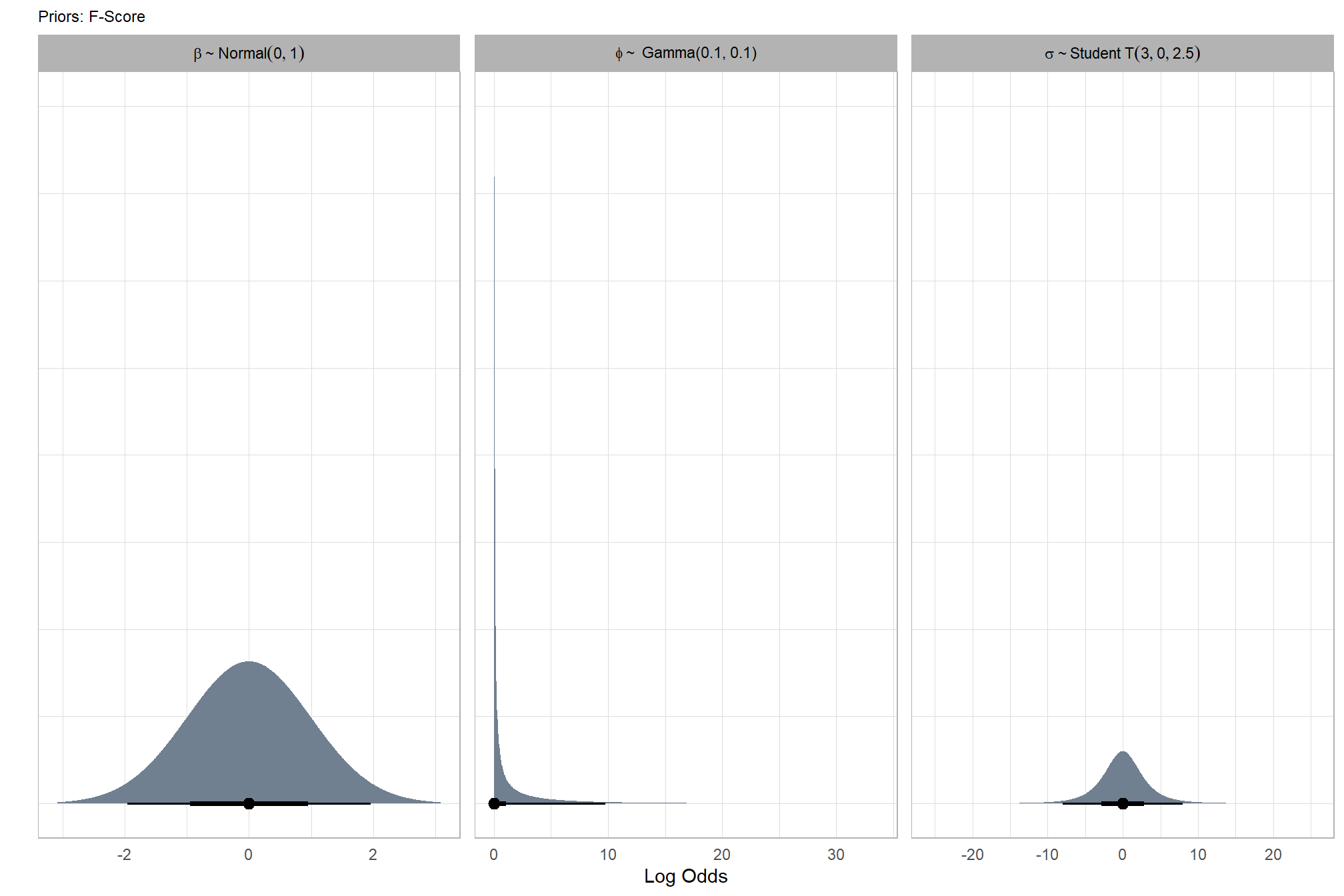
6.7.2.2 Fit the model
Now fit the model.
brms_f_mod5 = brms::brm(
  formula = f_score ~
    # baseline
    1 +
    # main effects
    (1 | depth_maps_generation_quality) +
    (1 | depth_maps_generation_filtering_mode) +
    (1 | software) +
    (1 | study_site) + # only fitting main effects of site and not interactions
    # two-way interactions
    (1 | depth_maps_generation_quality:depth_maps_generation_filtering_mode) +
    (1 | depth_maps_generation_quality:software) +
    (1 | depth_maps_generation_filtering_mode:software) +
    # three-way interactions
    (1 | depth_maps_generation_quality:depth_maps_generation_filtering_mode:software)
  , data = ptcld_validation_data
  , family = Beta(link = "logit")
  # priors
  , prior = brms_f_mod5_priors_temp
  # mcmc
  , iter = 20000, warmup = 10000, chains = 4
  , control = list(adapt_delta = 0.999, max_treedepth = 13)
  , cores = round(parallel::detectCores()/2)
  , file = paste0(rootdir, "/fits/brms_f_mod5")
)
# brms::make_stancode(brms_f_mod5)
# brms::prior_summary(brms_f_mod5)
# print(brms_f_mod5)
# brms::neff_ratio(brms_f_mod5)
# brms::rhat(brms_f_mod5)
# brms::nuts_params(brms_f_mod5)
check the prior distributions
# check priors
brms::prior_summary(brms_f_mod5) %>%
  kableExtra::kbl() %>%
kableExtra::kable_styling()| prior | class | coef | group | resp | dpar | nlpar | lb | ub | source |
|---|---|---|---|---|---|---|---|---|---|
| normal(0, 1) | Intercept | user | |||||||
| gamma(0.1, 0.1) | phi | 0 | user | ||||||
| student_t(3, 0, 2.5) | sd | 0 | user | ||||||
| sd | depth_maps_generation_filtering_mode | default | |||||||
| sd | Intercept | depth_maps_generation_filtering_mode | default | ||||||
| sd | depth_maps_generation_filtering_mode:software | default | |||||||
| sd | Intercept | depth_maps_generation_filtering_mode:software | default | ||||||
| sd | depth_maps_generation_quality | default | |||||||
| sd | Intercept | depth_maps_generation_quality | default | ||||||
| sd | depth_maps_generation_quality:depth_maps_generation_filtering_mode | default | |||||||
| sd | Intercept | depth_maps_generation_quality:depth_maps_generation_filtering_mode | default | ||||||
| sd | depth_maps_generation_quality:depth_maps_generation_filtering_mode:software | default | |||||||
| sd | Intercept | depth_maps_generation_quality:depth_maps_generation_filtering_mode:software | default | ||||||
| sd | depth_maps_generation_quality:software | default | |||||||
| sd | Intercept | depth_maps_generation_quality:software | default | ||||||
| sd | software | default | |||||||
| sd | Intercept | software | default | ||||||
| sd | study_site | default | |||||||
| sd | Intercept | study_site | default |
The brms::brm model summary
We won’t clutter the output here but this can be run if you are following along on your own
brms_f_mod5 %>%
  brms::posterior_summary() %>%
  as.data.frame() %>%
  tibble::rownames_to_column(var = "parameter") %>%
  dplyr::rename_with(tolower) %>%
  dplyr::filter(
    stringr::str_starts(parameter, "b_")
    | stringr::str_starts(parameter, "r_")
    | stringr::str_starts(parameter, "sd_")
    | parameter == "phi"
  ) %>%
  dplyr::mutate(
    parameter = parameter %>%
      stringr::str_replace_all("depth_maps_generation_quality", "quality") %>%
      stringr::str_replace_all("depth_maps_generation_filtering_mode", "filtering")
  ) %>%
  kableExtra::kbl(digits = 2, caption = "Bayesian final model for F-score") %>%
  kableExtra::kable_styling() %>%
  kableExtra::scroll_box(height = "8in")
6.7.2.3 Posterior Predictive Checks
Markov chain Monte Carlo (MCMC) simulations were conducted using the brms package (Bürkner 2017) to estimate posterior predictive distributions of the parameters of interest. We ran three chains of 100,000 iterations with the first 50,000 discarded as burn-in. Trace-plots were utilized to visually assess model convergence.
check the trace plots for problems with convergence of the Markov chains
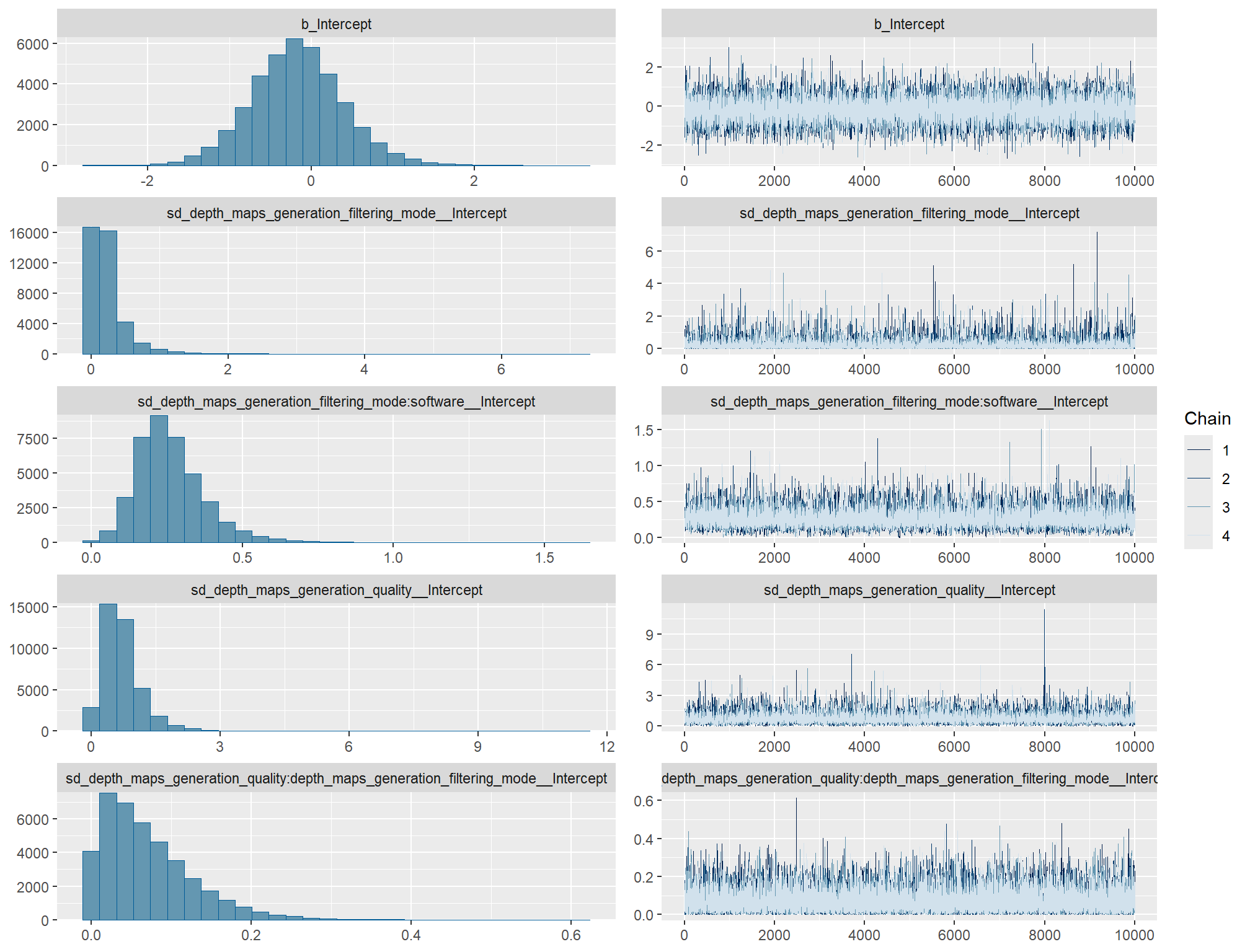
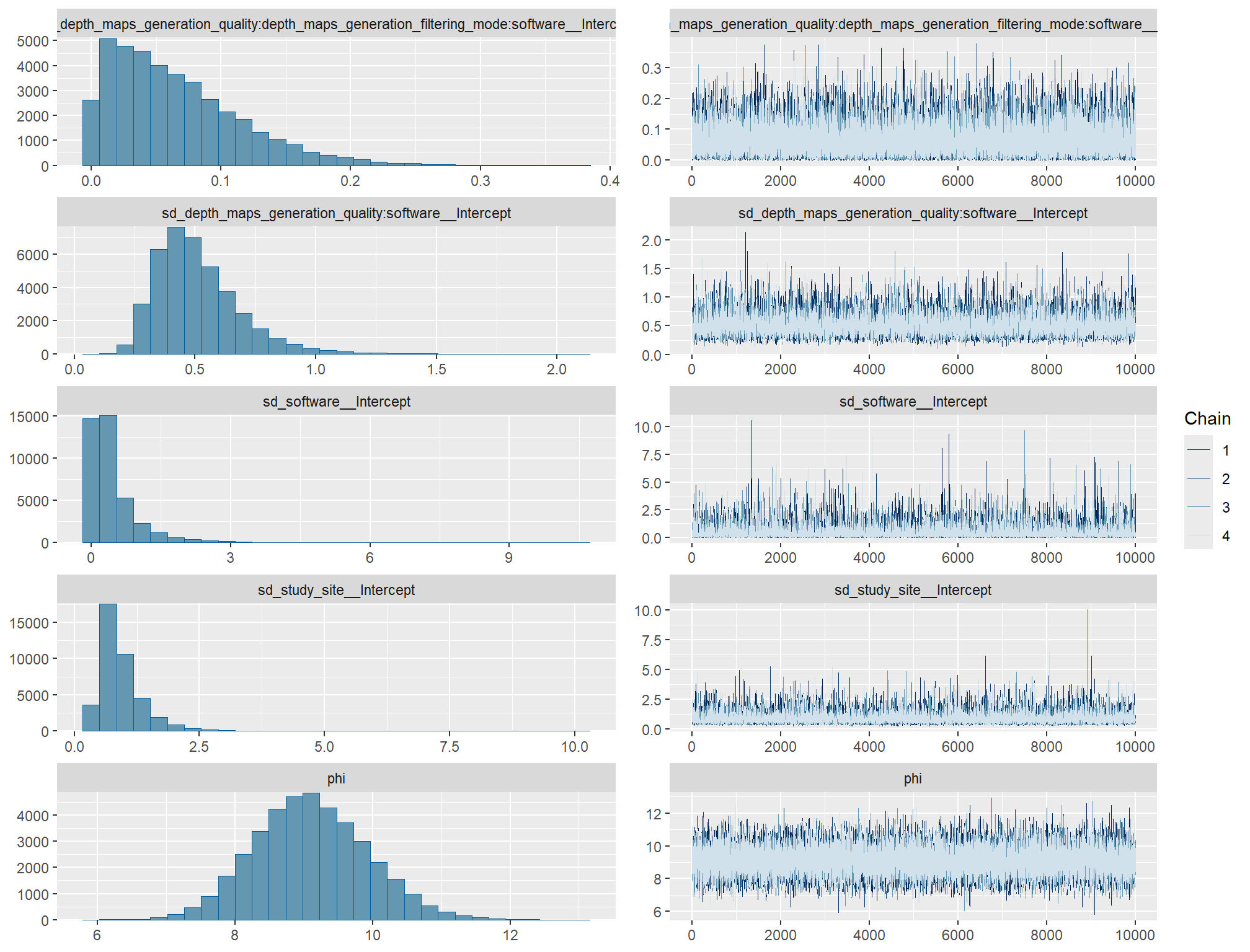
Sufficient convergence was checked with \(\hat{R}\) values near 1 (Brooks & Gelman, 1998).
check our \(\hat{R}\) values
brms::mcmc_plot(brms_f_mod5, type = "rhat_hist") +
  theme_light() +
  theme(
    legend.position = "top", legend.direction = "horizontal"
  )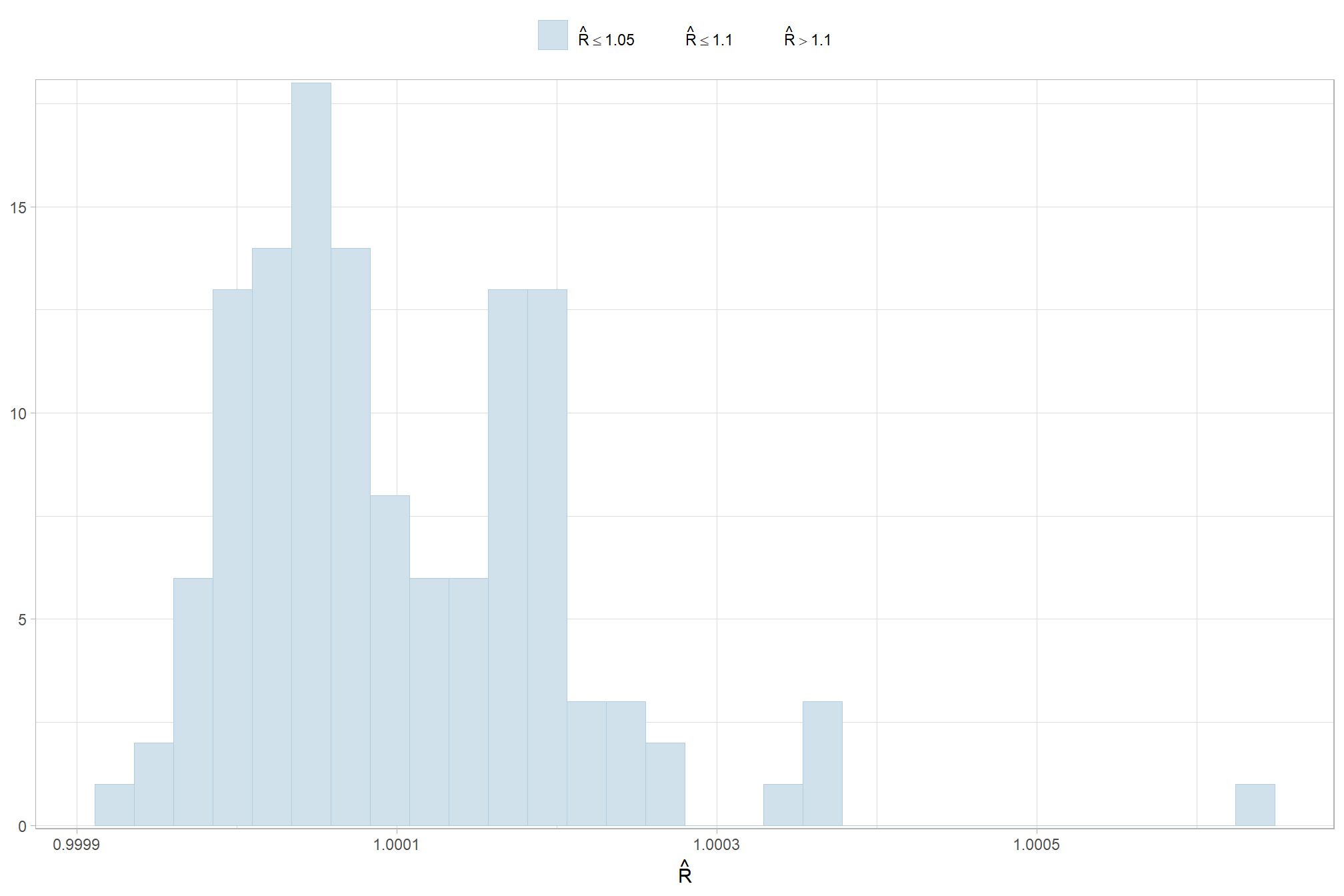
and another check of our \(\hat{R}\) values
brms_f_mod5 %>%
  brms::rhat() %>%
  as.data.frame() %>%
  tibble::rownames_to_column(var = "parameter") %>%
  dplyr::rename_with(tolower) %>%
  dplyr::rename(rhat = 2) %>%
  dplyr::filter(
    stringr::str_starts(parameter, "b_")
    | stringr::str_starts(parameter, "r_")
    | stringr::str_starts(parameter, "sd_")
    | parameter == "phi"
  ) %>%
  dplyr::mutate(
    parameter = parameter %>%
      stringr::str_replace_all("depth_maps_generation_quality", "quality") %>%
      stringr::str_replace_all("depth_maps_generation_filtering_mode", "filtering")
    , chk = (rhat <= 1*0.998 | rhat >= 1*1.002)
  ) %>%
  ggplot(aes(x = rhat, y = parameter, color = chk, fill = chk)) +
  geom_vline(xintercept = 1, linetype = "dashed", color = "gray44", lwd = 1.2) +
  geom_vline(xintercept = 1*0.998, lwd = 1.5) +
  geom_vline(xintercept = 1*1.002, lwd = 1.5) +
  geom_vline(xintercept = 1*0.999, lwd = 1.2, color = "gray33") +
  geom_vline(xintercept = 1*1.001, lwd = 1.2, color = "gray33") +
  geom_point() +
  scale_fill_manual(values = c("navy", "firebrick")) +
  scale_color_manual(values = c("navy", "firebrick")) +
  scale_y_discrete(NULL, breaks = NULL) +
  labs(
    x = latex2exp::TeX("$\\hat{R}$")
    , subtitle = latex2exp::TeX("MCMC chain convergence check for $\\hat{R}$ values")
    , title = "F-Score"
  ) +
  theme_light() +
  theme(
    legend.position = "none"
    , axis.text.y = element_text(size = 4)
    , panel.grid.major.x = element_blank()
    , panel.grid.minor.x = element_blank()
    , plot.subtitle = element_text(size = 8)
    , plot.title = element_text(size = 9)
  )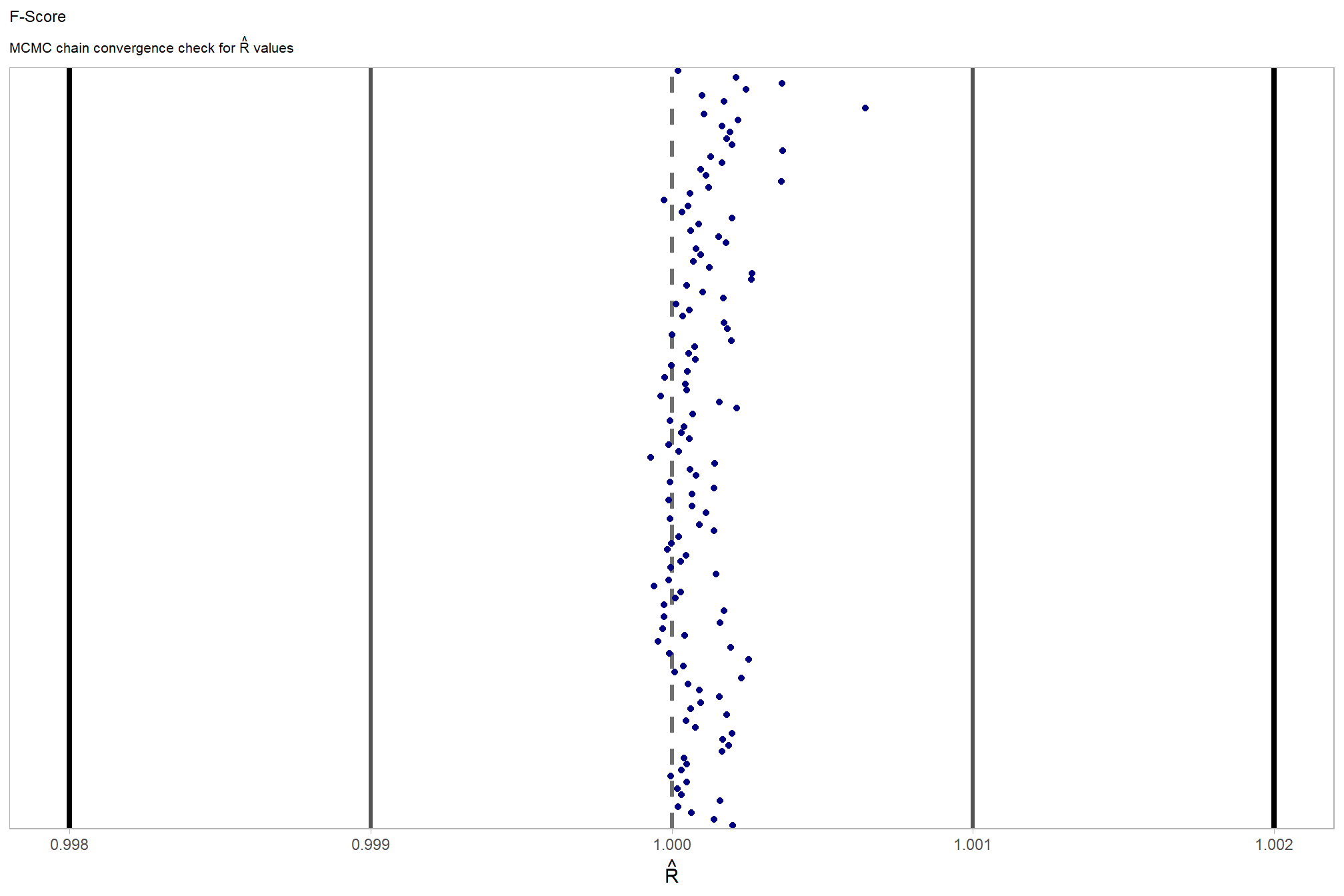
The effective length of an MCMC chain is indicated by the effective sample size (ESS), which refers to the sample size of the MCMC chain not to the sample size of the data Kruschke (2015) notes:
One simple guideline is this: For reasonably accurate and stable estimates of the limits of the 95% HDI, an ESS of 10,000 is recommended. This is merely a heuristic based on experience with practical applications, it is not a requirement. If accuracy of the HDI limits is not crucial for your application, then a smaller ESS may be sufficient. (p.184)
# get ess values from model summary
dplyr::bind_rows(
    summary(brms_f_mod5) %>%
      purrr::pluck("random") %>%
      purrr::flatten() %>%
      purrr::keep_at(~ .x == "Bulk_ESS") %>%
      unlist() %>%
      dplyr::as_tibble()
    , summary(brms_f_mod5) %>%
      purrr::pluck("fixed") %>%
      purrr::flatten() %>%
      purrr::keep_at(~ .x == "Bulk_ESS") %>%
      unlist() %>%
      dplyr::as_tibble()
  ) %>%
  dplyr::rename(ess = 1) %>%
  dplyr::mutate(parameter = dplyr::row_number(), chk = ess<10000) %>%
  ggplot(aes(x = ess, y = parameter, color = chk, fill = chk)) +
  geom_vline(xintercept = 10000, linetype = "dashed", color = "gray44", lwd = 1.2) +
  geom_segment( aes(x = 0, xend=ess, yend=parameter), color="black") +
  geom_point() +
  scale_fill_manual(values = c("blue4", "blue3")) +
  scale_color_manual(values = c("blue4", "blue3")) +
  scale_y_continuous(NULL, breaks = NULL) +
  scale_x_continuous(labels = scales::comma) +
  labs(
    x = "ESS"
    , subtitle = "MCMC chain resolution check for effective sample size (ESS) values"
    , y = ""
    , title = "F-Score"
  ) +
  theme_light() +
  theme(
    legend.position = "none"
    , axis.text.y = element_text(size = 4)
    , panel.grid.major.x = element_blank()
    , panel.grid.minor.x = element_blank()
    , plot.subtitle = element_text(size = 8)
    , plot.title = element_text(size = 9)
  )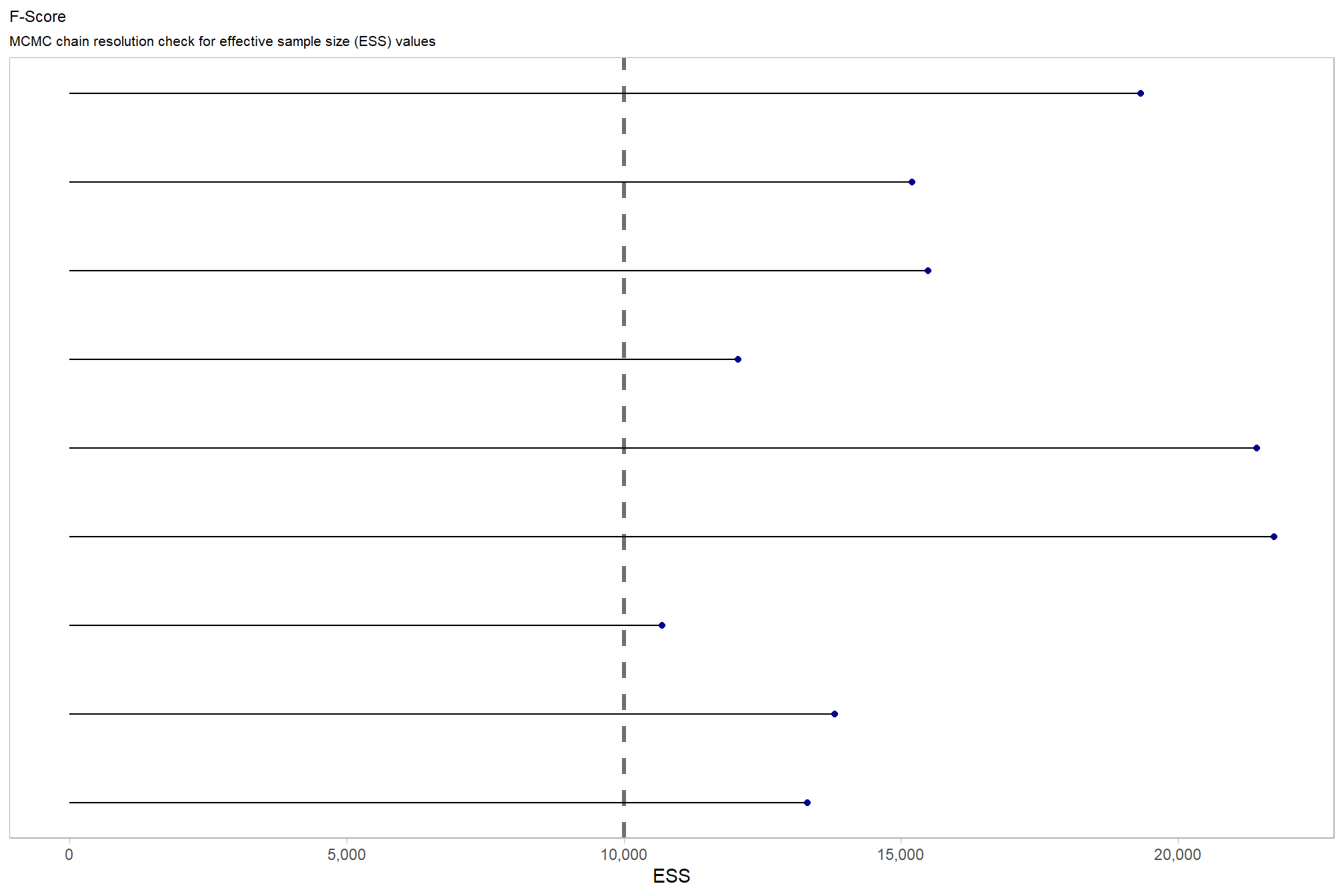
and another effective sample size check
brms::mcmc_plot(brms_f_mod5, type = "neff_hist") +
  theme_light() +
  theme(
    legend.position = "top", legend.direction = "horizontal"
  )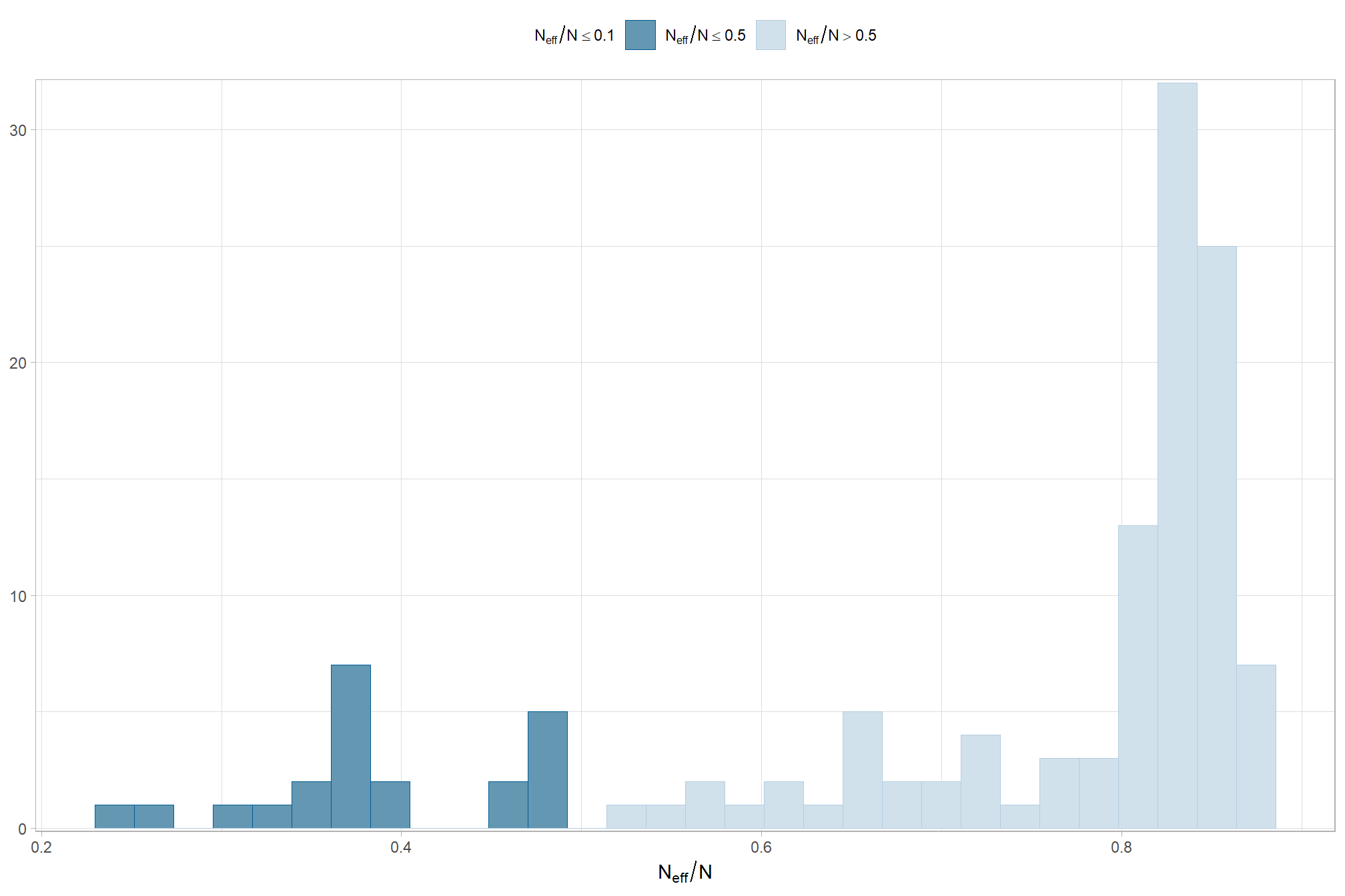
Posterior predictive checks were used to evaluate model goodness-of-fit by comparing data simulated from the model with the observed data used to estimate the model parameters (Hobbs & Hooten, 2015). Calculating the proportion of MCMC iterations in which the test statistic (i.e., mean and sum of squares) from the simulated data and observed data are more extreme than one another provides the Bayesian P-value. Lack of fit is indicated by a value close to 0 or 1 while a value of 0.5 indicates perfect fit (Hobbs & Hooten, 2015).
To learn more about this approach to posterior predictive checks, check out Gabry’s (2022) vignette, Graphical posterior predictive checks using the bayesplot package.
posterior-predictive check to make sure the model does an okay job simulating data that resemble the sample data
# posterior predictive check
brms::pp_check(
    brms_f_mod5
    , type = "dens_overlay"
    , ndraws = 100
  ) +
  labs(subtitle = "posterior-predictive check (overlaid densities)") +
  theme_light() +
  scale_y_continuous(NULL, breaks = NULL) +
  theme(
    legend.position = "top", legend.direction = "horizontal"
    , legend.text = element_text(size = 14)
    , plot.subtitle = element_text(size = 8)
    , plot.title = element_text(size = 9)
  )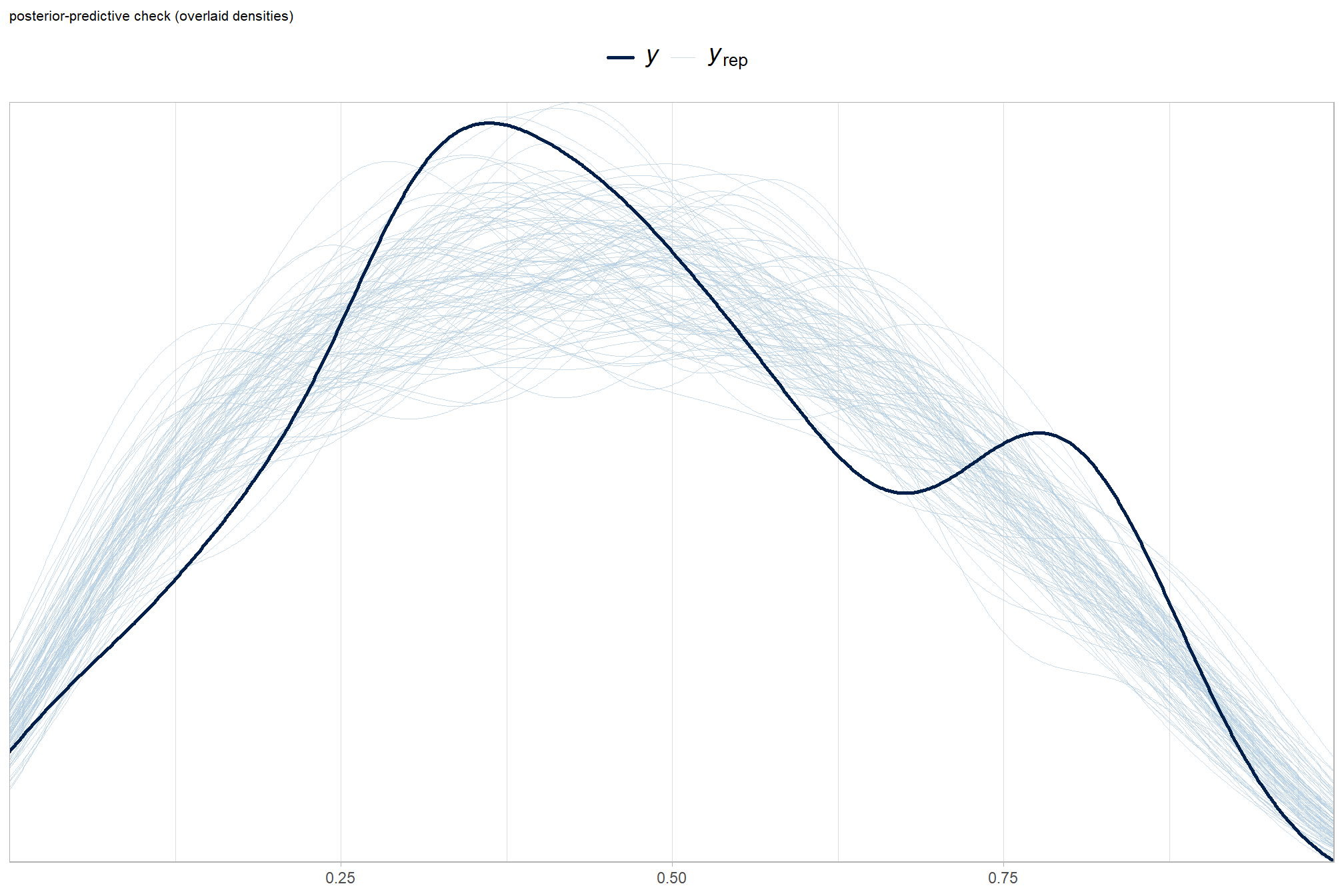
another way
brms::pp_check(brms_f_mod5, type = "ecdf_overlay", ndraws = 100) +
  labs(subtitle = "posterior-predictive check (ECDF: empirical cumulative distribution function)") +
  theme_light() +
  theme(
    legend.position = "top", legend.direction = "horizontal"
    , legend.text = element_text(size = 14)
  )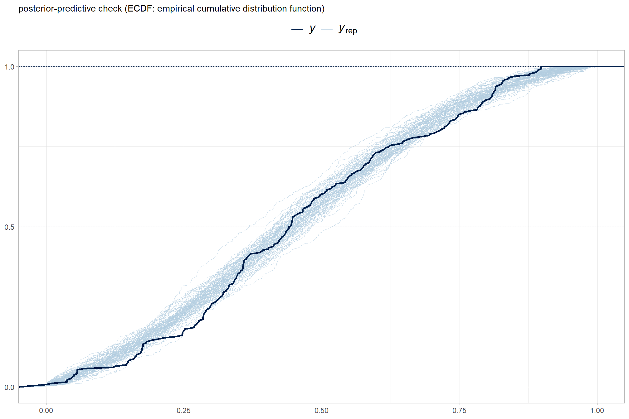
and another posterior predictive check for the overall model
# means
p1_temp = brms::pp_check(
    brms_f_mod5
    , type = "stat"
    , stat = "mean"
  ) +
  scale_y_continuous(NULL, breaks = c(NULL)) +
  labs(subtitle = "means") +
  theme_light()
# sds
p2_temp = brms::pp_check(
    brms_f_mod5
    , type = "stat"
    , stat = "sd"
  ) +
  scale_y_continuous(NULL, breaks = c(NULL)) +
  labs(subtitle = "sd's") +
  theme_light()

# combine
(p1_temp + p2_temp) &
  theme(legend.position = "none") &
  plot_annotation(
    title = "Posterior-predictive statistical checks\noverall model"
    , subtitle = expression(
      "The dark blue lines are "*italic(T(y))*", and the light blue bars are for "*italic(T)(italic(y)[rep])*".")
  )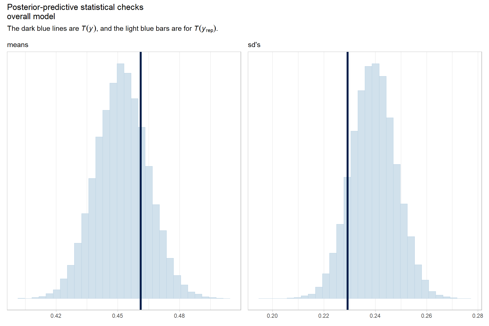
and another posterior predictive check for the overall model combining mean and sd
brms::pp_check(brms_f_mod5, type = "stat_2d") +
  theme_light() +
  labs(title = "F-Score") +
  theme(
    legend.position = "top", legend.direction = "horizontal"
    , legend.text = element_text(size = 8)
    , plot.title = element_text(size = 9)
  )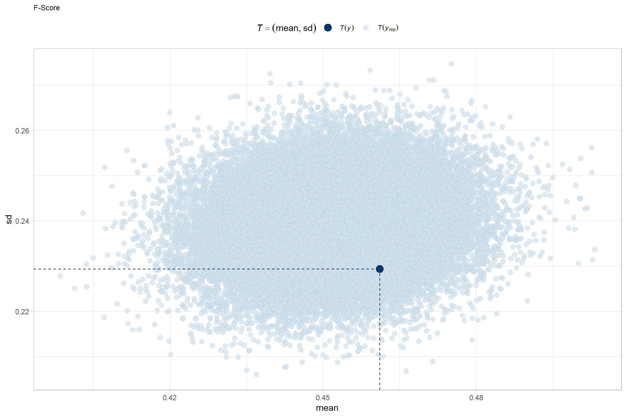
How’d we do capturing the conditional means and standard deviations by depth map generation quality?
# means
p1_temp = brms::pp_check(
    brms_f_mod5
    , type = "stat_grouped" # "dens_overlay_grouped"
    , stat = "mean"
    , group = "depth_maps_generation_quality"
  ) +
  scale_y_continuous(NULL, breaks = c(NULL)) +
  labs(subtitle = "means") +
  facet_grid(cols = vars(group), scales = "free") +
  theme_light()
# sds
p2_temp = brms::pp_check(
    brms_f_mod5
    , type = "stat_grouped" # "dens_overlay_grouped"
    , stat = "sd"
    , group = "depth_maps_generation_quality"
  ) +
  scale_y_continuous(NULL, breaks = c(NULL)) +
  labs(subtitle = "sd's") +
  facet_grid(cols = vars(group), scales = "free") +
  theme_light()
# combine
(p1_temp / p2_temp) &
  theme(legend.position = "none") &
  plot_annotation(
    title = "Posterior-predictive statistical checks\nby dense cloud quality"
    , subtitle = expression(
      "The dark blue lines are "*italic(T(y))*", and the light blue bars are for "*italic(T)(italic(y)[rep])*".")
  )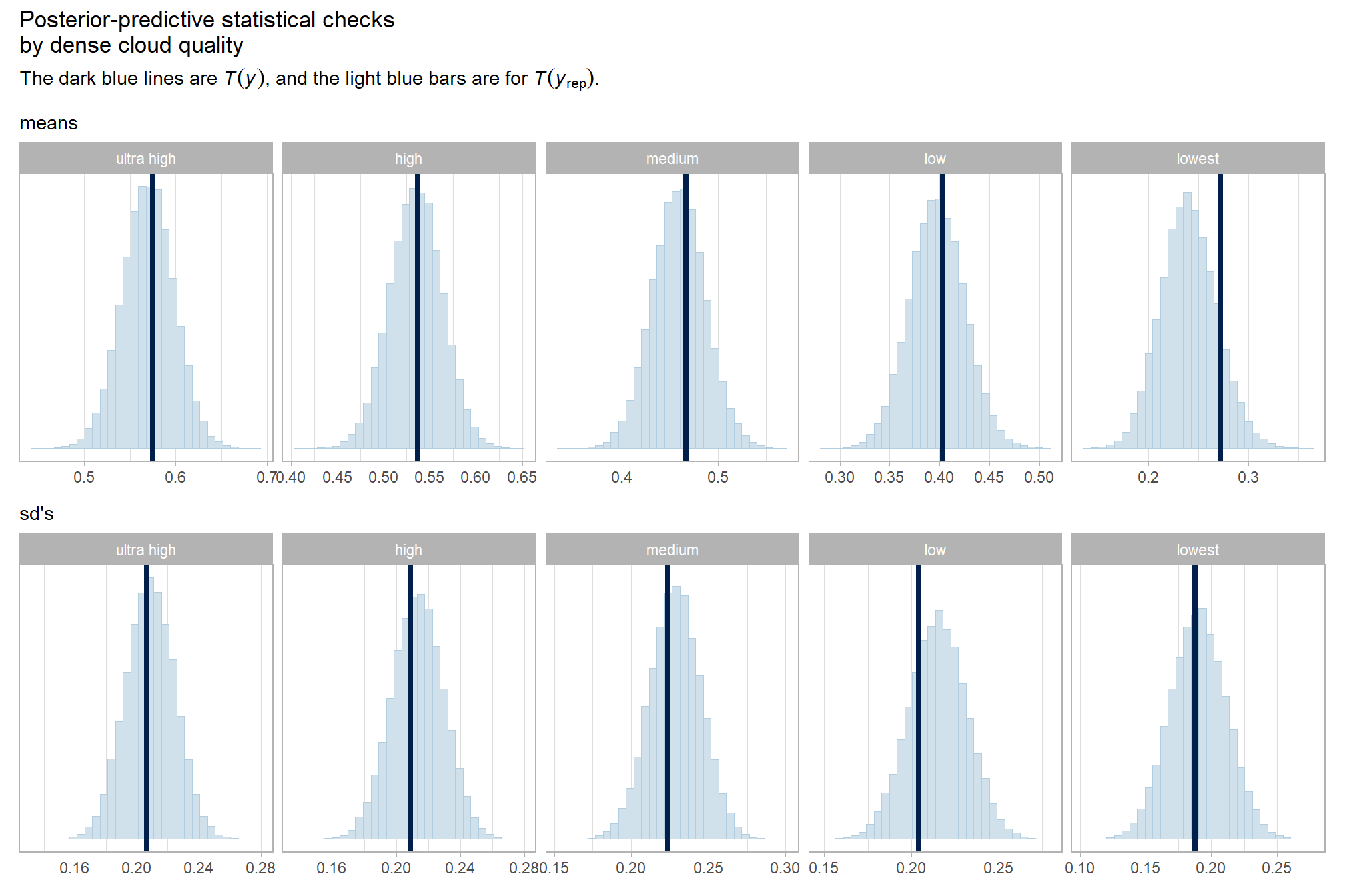
Both the means and sd’s of the F-score are well represented across the different levels of dense cloud quality
What about for the software?
pp_check(brms_f_mod5, "dens_overlay_grouped", group = "software", ndraws = 100) +
  labs(subtitle = "posterior-predictive check (overlaid densities)\nby software") +
  theme_light() +
  scale_y_continuous(NULL, breaks = NULL) +
  theme(
    legend.position = "top", legend.direction = "horizontal"
    , legend.text = element_text(size = 14)
  )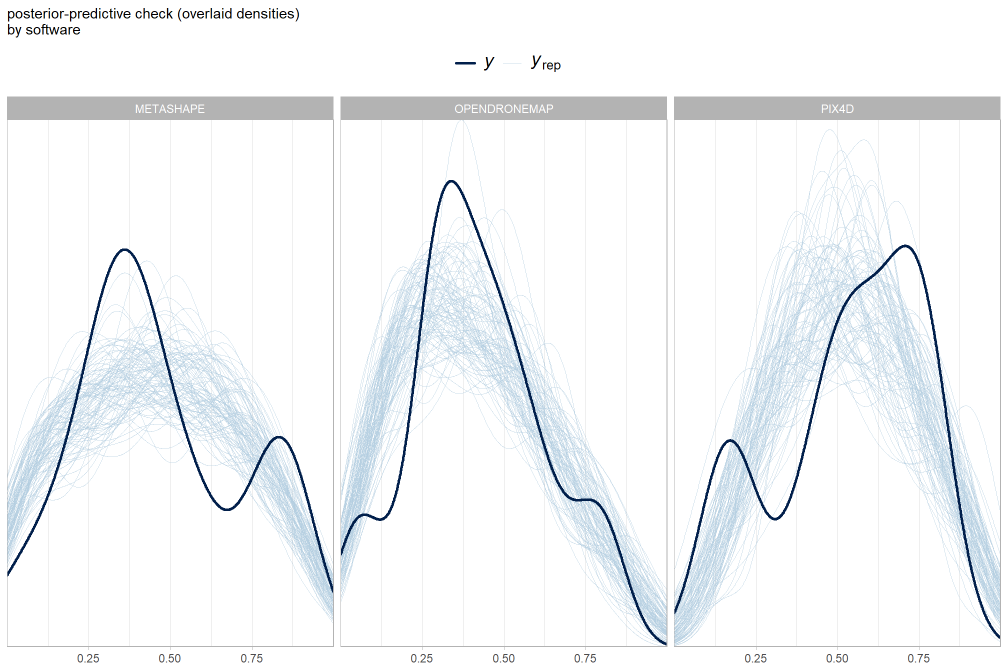
and what about for the filtering mode?
pp_check(brms_f_mod5, "dens_overlay_grouped", group = "depth_maps_generation_filtering_mode", ndraws = 100) +
  labs(subtitle = "posterior-predictive check (overlaid densities)\nby filtering mode") +
  theme_light() +
  scale_y_continuous(NULL, breaks = NULL) +
  theme(
    legend.position = "top", legend.direction = "horizontal"
    , legend.text = element_text(size = 14)
  )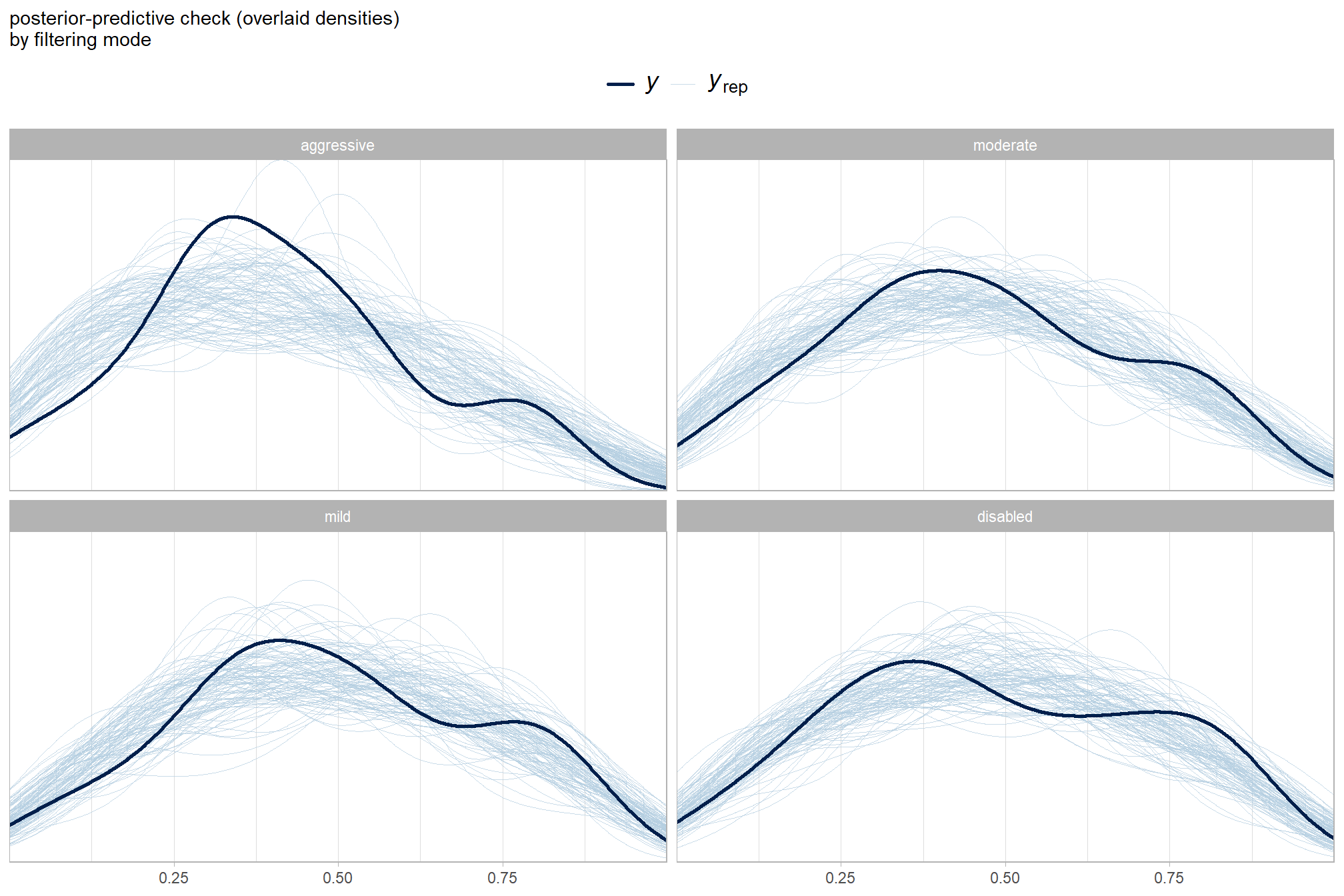
It looks like our model is making predictions that are consistent with our original data, which is what we want.
We can look at the model noise standard deviation (concentration) \(\phi\) and the intercept
We can think of mean (\(\mu\)) and precision (\(\phi\)) just like with a normal distribution and its mean and standard deviation.
# get formula
form_temp = brms_f_mod5$formula$formula[3] %>%
  as.character() %>% get_frmla_text() %>%
  stringr::str_replace_all("depth_maps_generation_quality", "quality") %>%
  stringr::str_replace_all("depth_maps_generation_filtering_mode", "filtering")
# extract the posterior draws
brms::as_draws_df(brms_f_mod5) %>%
# plot
  ggplot(aes(x = phi, y = 0)) +
  tidybayes::stat_dotsinterval(
    point_interval = median_hdi, .width = .95
    , justification = -0.04
    , shape = 21, point_size = 3
    , quantiles = 100
  ) +
  scale_y_continuous(NULL, breaks = NULL) +
  labs(
    x = latex2exp::TeX("$\\phi$")
    # , caption = form_temp
  ) +
  theme_light()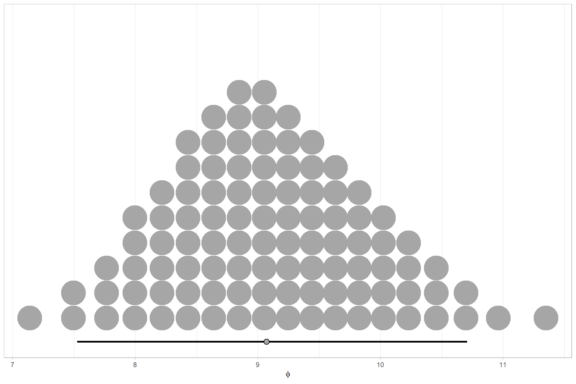
6.7.2.4 Quality:Filtering - interaction
Are there differences in F-score based on dense point cloud generation quality within each level of filtering mode?
Here, we collapse across the study site and software to compare the combined dense cloud quality and filtering mode effect.
In a hierarchical model structure, we have to make use of the re_formula argument within tidybayes::add_epred_draws
qlty_filter_draws_temp =
  ptcld_validation_data %>%
    dplyr::distinct(depth_maps_generation_quality, depth_maps_generation_filtering_mode) %>%
    tidybayes::add_epred_draws(
      brms_f_mod5, allow_new_levels = T
      # this part is crucial
      , re_formula = ~ (1 | depth_maps_generation_quality) +
        (1 | depth_maps_generation_filtering_mode) +
        (1 | depth_maps_generation_quality:depth_maps_generation_filtering_mode)
    ) %>%
    dplyr::rename(value = .epred) %>%
    dplyr::mutate(med = tidybayes::median_hdci(value)$y)
# plot
  qlty_filter_draws_temp %>%
    dplyr::mutate(depth_maps_generation_quality = depth_maps_generation_quality %>% forcats::fct_rev()) %>%
  # plot
  ggplot(
    mapping = aes(
      y = value, x = depth_maps_generation_filtering_mode
      # , fill = depth_maps_generation_filtering_mode
      , fill = med
    )
  ) +
    tidybayes::stat_eye(
      point_interval = median_hdi, .width = .95
      , slab_alpha = 0.95
      , interval_color = "black", linewidth = 1
      , point_color = "black", point_fill = "black", point_size = 1
    ) +
    # scale_fill_viridis_d(option = "plasma", drop = F) +
    scale_fill_viridis_c(option = "mako", direction=-1, begin = 0.2, end = 0.8, limits = c(0,1)) +
    scale_y_continuous(limits = c(0,1), breaks = scales::extended_breaks(n=8)) +
    facet_grid(cols = vars(depth_maps_generation_quality)) +
    labs(
      x = "filtering mode", y = "F-score"
      , subtitle = "posterior predictive distribution of F-score with 95% HDI\nby dense cloud quality"
      , fill = "Filtering Mode"
      # , caption = form_temp
    ) +
    theme_light() +
    theme(
      legend.position = "none"
      , legend.direction  = "horizontal"
      , axis.text.x = element_text(angle = 90, vjust = 0.5, hjust = 1)
      , strip.text = element_text(color = "black", face = "bold")
) 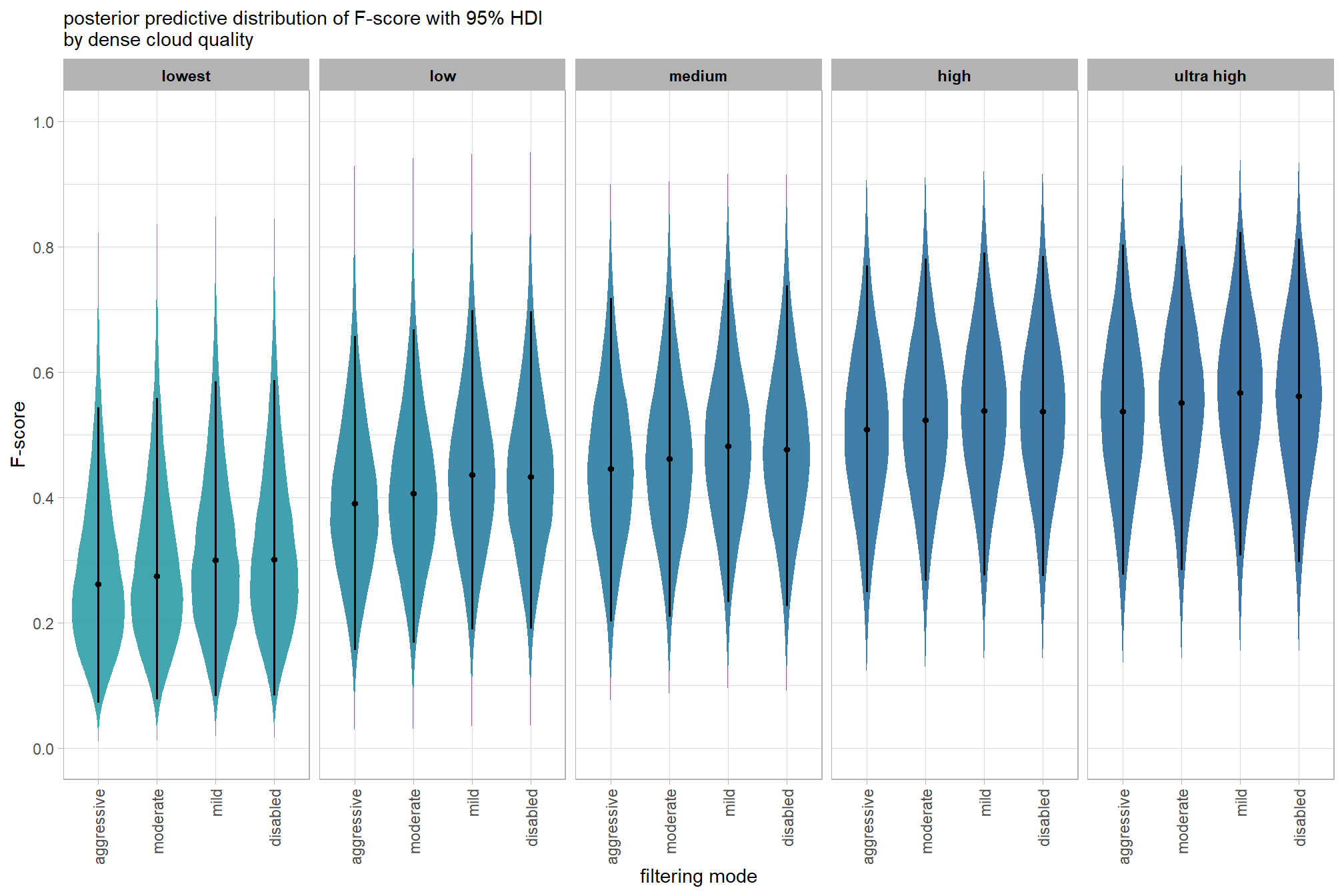
ggplot2::ggsave(
  "../data/qlty_fltr_mod5.png"
  , plot = ggplot2::last_plot() + labs(subtitle = "")
  , height = 7, width = 10.5
)
and a table of these 95% HDI values
table_temp =
  qlty_filter_draws_temp %>%
    tidybayes::median_hdi(value) %>%
    dplyr::select(-c(.point,.interval, .width,.row)) %>%
    dplyr::arrange(depth_maps_generation_quality, depth_maps_generation_filtering_mode)

table_temp %>%
  dplyr::select(-c(depth_maps_generation_quality)) %>%
  kableExtra::kbl(
    digits = 2
    , caption = "F-score<br>95% HDI of the posterior predictive distribution"
    , col.names = c(
      "filtering mode"
      , "F-score<br>median"
      , "HDI low", "HDI high"
    )
    , escape = F
  ) %>%
  kableExtra::kable_styling() %>%
  kableExtra::pack_rows(index = table(forcats::fct_inorder(table_temp$depth_maps_generation_quality))) %>%
kableExtra::scroll_box(height = "8in")| filtering mode |
F-score median |
HDI low | HDI high |
|---|---|---|---|
| ultra high | |||
| aggressive | 0.54 | 0.28 | 0.80 |
| moderate | 0.55 | 0.28 | 0.80 |
| mild | 0.57 | 0.31 | 0.82 |
| disabled | 0.56 | 0.30 | 0.81 |
| high | |||
| aggressive | 0.51 | 0.25 | 0.77 |
| moderate | 0.52 | 0.27 | 0.78 |
| mild | 0.54 | 0.28 | 0.79 |
| disabled | 0.54 | 0.27 | 0.79 |
| medium | |||
| aggressive | 0.45 | 0.20 | 0.72 |
| moderate | 0.46 | 0.21 | 0.72 |
| mild | 0.48 | 0.23 | 0.75 |
| disabled | 0.48 | 0.23 | 0.74 |
| low | |||
| aggressive | 0.39 | 0.16 | 0.66 |
| moderate | 0.41 | 0.17 | 0.67 |
| mild | 0.44 | 0.19 | 0.70 |
| disabled | 0.43 | 0.19 | 0.70 |
| lowest | |||
| aggressive | 0.26 | 0.07 | 0.54 |
| moderate | 0.28 | 0.08 | 0.56 |
| mild | 0.30 | 0.08 | 0.59 |
| disabled | 0.30 | 0.08 | 0.59 |
we can also make pairwise comparisons so long as we continue using tidybayes::add_epred_draws with the re_formula argument
brms_contrast_temp = qlty_filter_draws_temp %>%
    tidybayes::compare_levels(
      value
      , by = depth_maps_generation_quality
      , comparison =
        contrast_list
        # tidybayes::emmeans_comparison("revpairwise")
        #"pairwise"
    ) %>%
    dplyr::rename(contrast = depth_maps_generation_quality)

# separate contrast
brms_contrast_temp = brms_contrast_temp %>%
  dplyr::ungroup() %>%
  tidyr::separate_wider_delim(
    cols = contrast
    , delim = " - "
    , names = paste0(
        "sorter"
        , 1:(max(stringr::str_count(brms_contrast_temp$contrast, "-"))+1)
      )
    , too_few = "align_start"
    , cols_remove = F
  ) %>%
  dplyr::filter(sorter1!=sorter2) %>%
  dplyr::mutate(
    dplyr::across(
      tidyselect::starts_with("sorter")
      , .fns = function(x){factor(
        x, ordered = T
        , levels = levels(ptcld_validation_data$depth_maps_generation_quality)
      )}
    )
    , contrast = contrast %>%
      forcats::fct_reorder(
        paste0(as.numeric(sorter1), as.numeric(sorter2)) %>%
        as.numeric()
      )
    , depth_maps_generation_filtering_mode = depth_maps_generation_filtering_mode %>%
      factor(
        levels = levels(ptcld_validation_data$depth_maps_generation_filtering_mode)
        , ordered = T
      )
  ) %>%
  # median_hdi summary for coloring
  dplyr::group_by(contrast,depth_maps_generation_filtering_mode) %>%
  make_contrast_vars()

# what?
brms_contrast_temp %>% dplyr::glimpse()
## Rows: 1,600,000
## Columns: 19
## Groups: contrast, depth_maps_generation_filtering_mode [40]
## $ depth_maps_generation_filtering_mode <ord> aggressive, aggressive, aggressiv…
## $ .chain <int> NA, NA, NA, NA, NA, NA, NA, NA, N…
## $ .iteration <int> NA, NA, NA, NA, NA, NA, NA, NA, N…
## $ .draw <int> 1, 2, 3, 4, 5, 6, 7, 8, 9, 10, 11…
## $ sorter1 <ord> ultra high, ultra high, ultra hig…
## $ sorter2 <ord> high, high, high, high, high, hig…
## $ contrast <fct> ultra high - high, ultra high - h…
## $ value <dbl> -3.406868e-02, 7.723559e-02, 3.50…
## $ median_hdi_est <dbl> 0.02432316, 0.02432316, 0.0243231…
## $ median_hdi_lower <dbl> -0.1479552, -0.1479552, -0.147955…
## $ median_hdi_upper <dbl> 0.2016618, 0.2016618, 0.2016618, …
## $ pr_gt_zero <chr> "62%", "62%", "62%", "62%", "62%"…
## $ pr_lt_zero <chr> "38%", "38%", "38%", "38%", "38%"…
## $ is_diff_dir <lgl> FALSE, TRUE, TRUE, TRUE, TRUE, TR…
## $ pr_diff <dbl> 0.62375, 0.62375, 0.62375, 0.6237…
## $ pr_diff_lab <chr> "Pr(ultra high>high)=62%", "Pr(ul…
## $ pr_diff_lab_sm <chr> "Pr(>0)=62%", "Pr(>0)=62%", "Pr(>…
## $ pr_diff_lab_pos <dbl> 0.2167864, 0.2167864, 0.2167864, …
## $ sig_level <ord> <80%, <80%, <80%, <80%, <80%, <80…plot it
plt_contrast(
  brms_contrast_temp
  # , caption_text = form_temp
  , y_axis_title = "quality"
  , facet = "depth_maps_generation_filtering_mode"
  , label_size = 2.0
  , x_expand = c(0,0.6)
) +
  labs(
    subtitle = "posterior predictive distribution of group constrasts with 95% & 50% HDI\nby filtering mode"
  ) +
  theme(
    axis.text.x = element_text(size = 7)
  )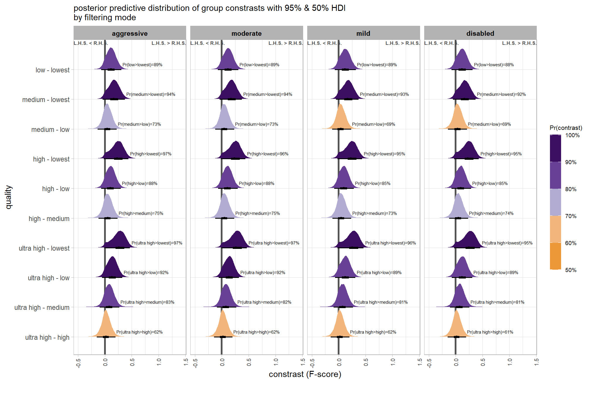
ggplot2::ggsave(
  "../data/qlty_fltr_comp_mod5.png"
  , plot = ggplot2::last_plot() + labs(subtitle = "")
  , height = 7, width = 10.5
)
and summarize these contrasts
table_temp =
  brms_contrast_temp %>%
  dplyr::group_by(contrast, depth_maps_generation_filtering_mode, pr_gt_zero) %>%
  tidybayes::median_hdi(value) %>%
  dplyr::arrange(contrast, depth_maps_generation_filtering_mode) %>%
  dplyr::select(contrast, depth_maps_generation_filtering_mode, value, .lower, .upper, pr_gt_zero) %>%
  dplyr::arrange(contrast, depth_maps_generation_filtering_mode)

table_temp %>%
  dplyr::select(-c(contrast)) %>%
kableExtra::kbl(
    digits = 2
    , caption = "brms::brm model: 95% HDI of the posterior predictive distribution of group constrasts"
    , col.names = c(
      "filtering mode"
      , "median difference<br>F-score"
      , "HDI low", "HDI high"
      , "Pr(diff>0)"
    )
    , escape = F
  ) %>%
  kableExtra::kable_styling() %>%
  kableExtra::pack_rows(index = table(forcats::fct_inorder(table_temp$contrast))) %>%
kableExtra::scroll_box(height = "8in")| filtering mode |
median difference F-score |
HDI low | HDI high | Pr(diff>0) |
|---|---|---|---|---|
| ultra high - high | ||||
| aggressive | 0.02 | -0.15 | 0.20 | 62% |
| moderate | 0.02 | -0.15 | 0.20 | 62% |
| mild | 0.02 | -0.15 | 0.20 | 62% |
| disabled | 0.02 | -0.15 | 0.20 | 61% |
| ultra high - medium | ||||
| aggressive | 0.08 | -0.10 | 0.27 | 83% |
| moderate | 0.08 | -0.09 | 0.27 | 82% |
| mild | 0.08 | -0.10 | 0.26 | 81% |
| disabled | 0.08 | -0.10 | 0.26 | 81% |
| ultra high - low | ||||
| aggressive | 0.14 | -0.05 | 0.33 | 92% |
| moderate | 0.14 | -0.06 | 0.32 | 92% |
| mild | 0.12 | -0.07 | 0.31 | 89% |
| disabled | 0.12 | -0.07 | 0.31 | 89% |
| ultra high - lowest | ||||
| aggressive | 0.26 | -0.01 | 0.47 | 97% |
| moderate | 0.27 | -0.01 | 0.47 | 97% |
| mild | 0.26 | -0.02 | 0.46 | 96% |
| disabled | 0.25 | -0.03 | 0.46 | 95% |
| high - medium | ||||
| aggressive | 0.06 | -0.12 | 0.24 | 75% |
| moderate | 0.05 | -0.12 | 0.23 | 75% |
| mild | 0.05 | -0.12 | 0.24 | 73% |
| disabled | 0.05 | -0.12 | 0.23 | 74% |
| high - low | ||||
| aggressive | 0.11 | -0.07 | 0.30 | 88% |
| moderate | 0.11 | -0.07 | 0.30 | 88% |
| mild | 0.10 | -0.08 | 0.28 | 85% |
| disabled | 0.10 | -0.08 | 0.29 | 85% |
| high - lowest | ||||
| aggressive | 0.23 | -0.02 | 0.44 | 97% |
| moderate | 0.24 | -0.02 | 0.44 | 96% |
| mild | 0.23 | -0.02 | 0.44 | 95% |
| disabled | 0.23 | -0.03 | 0.43 | 95% |
| medium - low | ||||
| aggressive | 0.05 | -0.13 | 0.22 | 73% |
| moderate | 0.05 | -0.12 | 0.23 | 73% |
| mild | 0.04 | -0.12 | 0.23 | 69% |
| disabled | 0.04 | -0.14 | 0.21 | 69% |
| medium - lowest | ||||
| aggressive | 0.17 | -0.04 | 0.37 | 94% |
| moderate | 0.17 | -0.04 | 0.37 | 94% |
| mild | 0.17 | -0.05 | 0.37 | 93% |
| disabled | 0.16 | -0.05 | 0.37 | 92% |
| low - lowest | ||||
| aggressive | 0.11 | -0.07 | 0.31 | 89% |
| moderate | 0.12 | -0.07 | 0.31 | 89% |
| mild | 0.12 | -0.07 | 0.32 | 89% |
| disabled | 0.12 | -0.07 | 0.32 | 88% |
6.7.2.5 Software:Quality - interaction
It might be more important to understand the difference in F-score by dense cloud quality and software rather than filtering mode since filtering mode had such a small effect on the SfM predictive ability
Are there differences in F-score based on dense point cloud generation quality within each different processing software? We will also address the similar but slightly different question of “are there differences in F-score based on the processing software used at a given dense point cloud generation quality?”
Here, we collapse across the study site and filtering mode to compare the combined dense cloud quality and software effect.
In a hierarchical model structure, we have to make use of the re_formula argument within tidybayes::add_epred_draws
# get draws
qlty_sftwr_draws_temp =
  tidyr::crossing(
    depth_maps_generation_quality = unique(ptcld_validation_data$depth_maps_generation_quality)
    , software = unique(ptcld_validation_data$software)
  ) %>%
  tidybayes::add_epred_draws(
    brms_f_mod5, allow_new_levels = T
    # this part is crucial
    , re_formula = ~ (1 | depth_maps_generation_quality) +
      (1 | software) +
      (1 | depth_maps_generation_quality:software)
  ) %>%
  dplyr::rename(value = .epred) %>%
  dplyr::mutate(
    med = tidybayes::median_hdci(value)$y
  )

# plot
qlty_sftwr_draws_temp %>%
  # remove out-of-sample obs
  dplyr::inner_join(
    ptcld_validation_data %>% dplyr::distinct(depth_maps_generation_quality, software)
    , by = dplyr::join_by(depth_maps_generation_quality, software)
  ) %>%
  dplyr::mutate(
    depth_maps_generation_quality = depth_maps_generation_quality %>% forcats::fct_rev()
  ) %>%
  # plot
  ggplot(
    mapping = aes(
      y = value, x = software
      # , fill = software
      , fill = med
    )
  ) +
  tidybayes::stat_eye(
    point_interval = median_hdi, .width = .95
    , slab_alpha = 0.95
    , interval_color = "black", linewidth = 1
    , point_color = "black", point_fill = "black", point_size = 1
  ) +
  # scale_fill_viridis_d(option = "rocket", begin = 0.3, end = 0.9, drop = F) +
  scale_fill_viridis_c(option = "mako", direction=-1, begin = 0.2, end = 0.8, limits = c(0,1)) +
  scale_y_continuous(limits = c(0,1), breaks = scales::extended_breaks(n=8)) +
  facet_grid(cols = vars(depth_maps_generation_quality)) +
  labs(
    x = "software", y = "F-score"
    , subtitle = "posterior predictive distribution of F-score with 95% HDI\nby dense cloud quality"
    # , caption = form_temp
  ) +
  theme_light() +
  theme(
    legend.position = "none"
    , legend.direction  = "horizontal"
    , axis.text.x = element_text(angle = 90, vjust = 0.5, hjust = 1)
    , strip.text = element_text(color = "black", face = "bold")
) 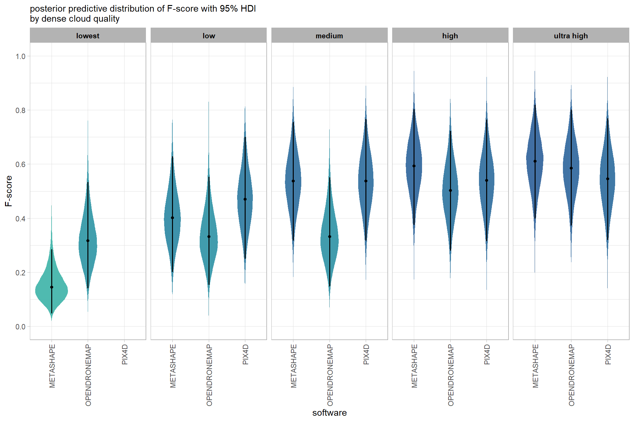
and a table of these 95% HDI values
table_temp =
  qlty_sftwr_draws_temp %>%
    tidybayes::median_hdi(value) %>%
    # remove out-of-sample obs
    dplyr::inner_join(
      ptcld_validation_data %>% dplyr::distinct(depth_maps_generation_quality, software)
      , by = dplyr::join_by(depth_maps_generation_quality, software)
    ) %>%
    dplyr::select(-c(.point,.interval, .width,.row)) %>%
    dplyr::arrange(software,depth_maps_generation_quality)

table_temp %>%
  dplyr::select(-c(software)) %>%
  kableExtra::kbl(
    digits = 2
    , caption = "F-score<br>95% HDI of the posterior predictive distribution"
    , col.names = c(
      "quality"
      , "F-score<br>median"
      , "HDI low", "HDI high"
    )
    , escape = F
  ) %>%
  kableExtra::kable_styling() %>%
  kableExtra::pack_rows(index = table(forcats::fct_inorder(table_temp$software))) %>%
kableExtra::scroll_box(height = "8in")| quality |
F-score median |
HDI low | HDI high |
|---|---|---|---|
| METASHAPE | |||
| ultra high | 0.61 | 0.40 | 0.82 |
| high | 0.59 | 0.38 | 0.80 |
| medium | 0.54 | 0.32 | 0.76 |
| low | 0.40 | 0.20 | 0.63 |
| lowest | 0.15 | 0.05 | 0.28 |
| OPENDRONEMAP | |||
| ultra high | 0.59 | 0.37 | 0.80 |
| high | 0.50 | 0.28 | 0.72 |
| medium | 0.33 | 0.15 | 0.55 |
| low | 0.33 | 0.15 | 0.55 |
| lowest | 0.32 | 0.14 | 0.53 |
| PIX4D | |||
| ultra high | 0.55 | 0.32 | 0.77 |
| high | 0.54 | 0.31 | 0.76 |
| medium | 0.54 | 0.32 | 0.77 |
| low | 0.47 | 0.25 | 0.70 |
we can also make pairwise comparisons so long as we continue using tidybayes::add_epred_draws with the re_formula argument
# calculate contrast
brms_contrast_temp = qlty_sftwr_draws_temp %>%
  tidybayes::compare_levels(
    value
    , by = depth_maps_generation_quality
    , comparison = contrast_list
  ) %>%
  dplyr::rename(contrast = depth_maps_generation_quality)

# separate contrast
brms_contrast_temp = brms_contrast_temp %>%
  dplyr::ungroup() %>%
  tidyr::separate_wider_delim(
    cols = contrast
    , delim = " - "
    , names = paste0(
      "sorter"
      , 1:(max(stringr::str_count(brms_contrast_temp$contrast, "-"))+1)
    )
    , too_few = "align_start"
    , cols_remove = F
  ) %>%
  dplyr::filter(sorter1!=sorter2) %>%
  dplyr::mutate(
    dplyr::across(
      tidyselect::starts_with("sorter")
      , .fns = function(x){factor(
        x, ordered = T
        , levels = levels(ptcld_validation_data$depth_maps_generation_quality)
      )}
    )
    , contrast = contrast %>%
      forcats::fct_reorder(
        paste0(as.numeric(sorter1), as.numeric(sorter2)) %>%
          as.numeric()
      )
  ) %>%
  # median_hdi summary for coloring
  dplyr::group_by(contrast, software) %>%
  make_contrast_vars()

# remove out-of-sample obs
brms_contrast_temp = brms_contrast_temp %>%
  dplyr::inner_join(
    ptcld_validation_data %>% dplyr::distinct(software, depth_maps_generation_quality)
    , by = dplyr::join_by(software, sorter1 == depth_maps_generation_quality)
  ) %>%
  dplyr::inner_join(
    ptcld_validation_data %>% dplyr::distinct(software, depth_maps_generation_quality)
    , by = dplyr::join_by(software, sorter2 == depth_maps_generation_quality)
  )

# what?
brms_contrast_temp %>% dplyr::glimpse()
## Rows: 1,040,000
## Columns: 19
## Groups: contrast, software [26]
## $ software <chr> "METASHAPE", "METASHAPE", "METASHAPE", "METASHAPE", "…
## $ .chain <int> NA, NA, NA, NA, NA, NA, NA, NA, NA, NA, NA, NA, NA, N…
## $ .iteration <int> NA, NA, NA, NA, NA, NA, NA, NA, NA, NA, NA, NA, NA, N…
## $ .draw <int> 1, 2, 3, 4, 5, 6, 7, 8, 9, 10, 11, 12, 13, 14, 15, 16…
## $ sorter1 <ord> ultra high, ultra high, ultra high, ultra high, ultra…
## $ sorter2 <ord> high, high, high, high, high, high, high, high, high,…
## $ contrast <fct> ultra high - high, ultra high - high, ultra high - hi…
## $ value <dbl> -0.0502782314, -0.0614947682, 0.0277093118, -0.073845…
## $ median_hdi_est <dbl> 0.01640508, 0.01640508, 0.01640508, 0.01640508, 0.016…
## $ median_hdi_lower <dbl> -0.08128401, -0.08128401, -0.08128401, -0.08128401, -…
## $ median_hdi_upper <dbl> 0.11623, 0.11623, 0.11623, 0.11623, 0.11623, 0.11623,…
## $ pr_gt_zero <chr> "63%", "63%", "63%", "63%", "63%", "63%", "63%", "63%…
## $ pr_lt_zero <chr> "37%", "37%", "37%", "37%", "37%", "37%", "37%", "37%…
## $ is_diff_dir <lgl> FALSE, FALSE, TRUE, FALSE, FALSE, TRUE, TRUE, FALSE, …
## $ pr_diff <dbl> 0.630175, 0.630175, 0.630175, 0.630175, 0.630175, 0.6…
## $ pr_diff_lab <chr> "Pr(ultra high>high)=63%", "Pr(ultra high>high)=63%",…
## $ pr_diff_lab_sm <chr> "Pr(>0)=63%", "Pr(>0)=63%", "Pr(>0)=63%", "Pr(>0)=63%…
## $ pr_diff_lab_pos <dbl> 0.1249473, 0.1249473, 0.1249473, 0.1249473, 0.1249473…
## $ sig_level <ord> <80%, <80%, <80%, <80%, <80%, <80%, <80%, <80%, <80%,…plot it
plt_contrast(
  brms_contrast_temp
  # , caption_text = form_temp
  , y_axis_title = "quality"
  , facet = "software"
  , label_size = 2.0
  , x_expand = c(0.56,0.9) # c(0,0.7)
) +
  labs(
    subtitle = "posterior predictive distribution of group constrasts with 95% & 50% HDI\nby software"
  )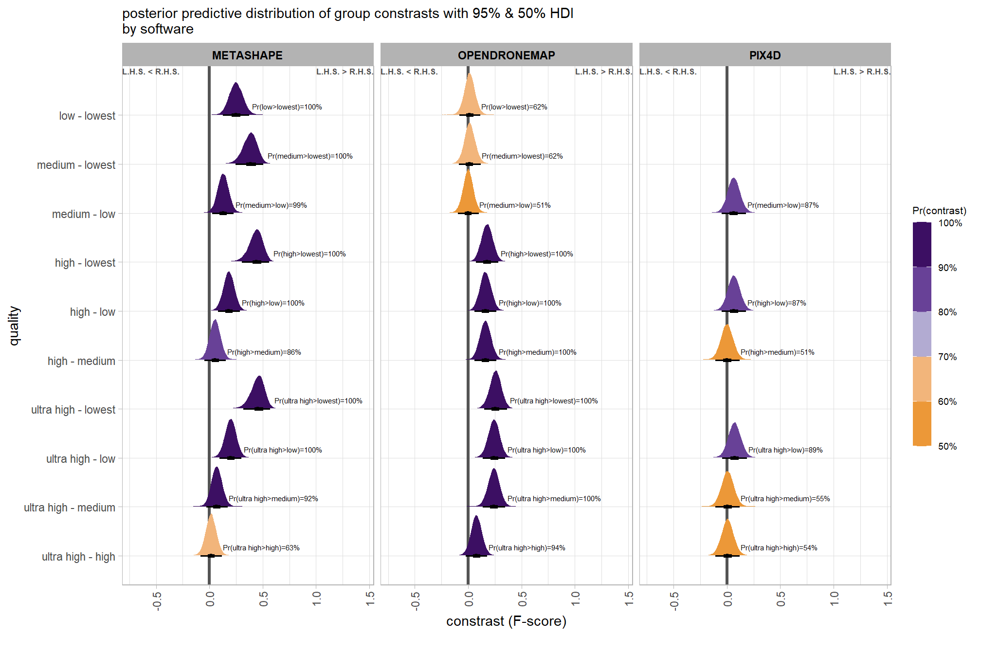
ggplot2::ggsave(
  "../data/qlty_sftwr_comp_mod5.png"
  , plot = ggplot2::last_plot() + labs(subtitle = "")
  , height = 7, width = 10.5
)
create plot for combining with other contrasts for publication
ptchwrk_qlty_sftwr_comp =
  plt_contrast(
    brms_contrast_temp
    , y_axis_title = "quality contrast"
    , facet = "software"
    , label_size = 1.35
    , label = "pr_diff_lab_sm"
    , annotate_size = 1.75
  ) +
    labs(
      subtitle = ""
      , x = "F-score contrast"
    ) +
    theme(
      legend.position="none"
      , axis.title.y = element_text(size = 10, face = "bold")
      , axis.title.x = element_text(size = 8)
    )
# ptchwrk_qlty_sftwr_comp
and summarize these contrasts
table_temp = brms_contrast_temp %>%
  dplyr::group_by(contrast, software, pr_gt_zero) %>%
  tidybayes::median_hdi(value) %>%
  dplyr::arrange(contrast, software) %>%
  dplyr::select(contrast, software, value, .lower, .upper, pr_gt_zero) %>%
  dplyr::arrange(software, contrast)

table_temp %>%
  dplyr::select(-c(software)) %>%
  kableExtra::kbl(
    digits = 2
    , caption = "brms::brm model: 95% HDI of the posterior predictive distribution of group constrasts"
    , col.names = c(
      "quality contrast"
      , "median difference<br>F-score"
      , "HDI low", "HDI high"
      , "Pr(diff>0)"
    )
    , escape = F
  ) %>%
  kableExtra::kable_styling() %>%
  kableExtra::pack_rows(index = table(forcats::fct_inorder(table_temp$software))) %>%
kableExtra::scroll_box(height = "8in")| quality contrast |
median difference F-score |
HDI low | HDI high | Pr(diff>0) |
|---|---|---|---|---|
| METASHAPE | ||||
| ultra high - high | 0.02 | -0.08 | 0.12 | 63% |
| ultra high - medium | 0.07 | -0.03 | 0.17 | 92% |
| ultra high - low | 0.20 | 0.09 | 0.30 | 100% |
| ultra high - lowest | 0.46 | 0.32 | 0.57 | 100% |
| high - medium | 0.05 | -0.04 | 0.15 | 86% |
| high - low | 0.18 | 0.08 | 0.28 | 100% |
| high - lowest | 0.44 | 0.30 | 0.56 | 100% |
| medium - low | 0.13 | 0.03 | 0.23 | 99% |
| medium - lowest | 0.38 | 0.25 | 0.51 | 100% |
| low - lowest | 0.25 | 0.13 | 0.37 | 100% |
| OPENDRONEMAP | ||||
| ultra high - high | 0.08 | -0.02 | 0.18 | 94% |
| ultra high - medium | 0.24 | 0.13 | 0.34 | 100% |
| ultra high - low | 0.24 | 0.14 | 0.35 | 100% |
| ultra high - lowest | 0.26 | 0.15 | 0.36 | 100% |
| high - medium | 0.16 | 0.06 | 0.27 | 100% |
| high - low | 0.16 | 0.06 | 0.27 | 100% |
| high - lowest | 0.18 | 0.07 | 0.28 | 100% |
| medium - low | 0.00 | -0.09 | 0.10 | 51% |
| medium - lowest | 0.01 | -0.09 | 0.12 | 62% |
| low - lowest | 0.01 | -0.08 | 0.12 | 62% |
| PIX4D | ||||
| ultra high - high | 0.01 | -0.11 | 0.12 | 54% |
| ultra high - medium | 0.01 | -0.11 | 0.12 | 55% |
| ultra high - low | 0.07 | -0.04 | 0.19 | 89% |
| high - medium | 0.00 | -0.11 | 0.12 | 51% |
| high - low | 0.06 | -0.05 | 0.18 | 87% |
| medium - low | 0.06 | -0.05 | 0.18 | 87% |
The contrasts above address the question “are there differences in F-score based on dense point cloud generation quality within each software?”.
To address the different question of “are there differences in F-score based on the processing software used at a given dense point cloud generation quality?” we need to utilize a different formulation of the comparison parameter within our call to the tidybayes::compare_levels function and calculate the contrast by software instead
# calculate contrast
brms_contrast_temp = qlty_sftwr_draws_temp %>%
  tidybayes::compare_levels(
    value
    , by = software
    , comparison = "pairwise"
  ) %>%
  dplyr::rename(contrast = software) %>%
  # median_hdi summary for coloring
  dplyr::group_by(contrast, depth_maps_generation_quality) %>%
  make_contrast_vars()

# remove out-of-sample obs
brms_contrast_temp = brms_contrast_temp %>%
  tidyr::separate_wider_delim(
    cols = contrast
    , delim = " - "
    , names = paste0(
      "sorter"
      , 1:(max(stringr::str_count(brms_contrast_temp$contrast, "-"))+1)
    )
    , too_few = "align_start"
    , cols_remove = F
  ) %>%
  dplyr::filter(sorter1!=sorter2) %>%
  dplyr::inner_join(
    ptcld_validation_data %>% dplyr::distinct(software, depth_maps_generation_quality)
    , by = dplyr::join_by(sorter1 == software, depth_maps_generation_quality)
  ) %>%
  dplyr::inner_join(
    ptcld_validation_data %>% dplyr::distinct(software, depth_maps_generation_quality)
    , by = dplyr::join_by(sorter2 == software, depth_maps_generation_quality)
  )
# what?
brms_contrast_temp %>% dplyr::glimpse()
## Rows: 520,000
## Columns: 19
## Groups: contrast, depth_maps_generation_quality [13]
## $ depth_maps_generation_quality <ord> ultra high, ultra high, ultra high, ultr…
## $ .chain <int> NA, NA, NA, NA, NA, NA, NA, NA, NA, NA, …
## $ .iteration <int> NA, NA, NA, NA, NA, NA, NA, NA, NA, NA, …
## $ .draw <int> 1, 2, 3, 4, 5, 6, 7, 8, 9, 10, 11, 12, 1…
## $ sorter1 <chr> "OPENDRONEMAP", "OPENDRONEMAP", "OPENDRO…
## $ sorter2 <chr> "METASHAPE", "METASHAPE", "METASHAPE", "…
## $ contrast <chr> "OPENDRONEMAP - METASHAPE", "OPENDRONEMA…
## $ value <dbl> 0.042159383, 0.026812062, -0.048880389, …
## $ median_hdi_est <dbl> -0.02460791, -0.02460791, -0.02460791, -…
## $ median_hdi_lower <dbl> -0.14867, -0.14867, -0.14867, -0.14867, …
## $ median_hdi_upper <dbl> 0.09981064, 0.09981064, 0.09981064, 0.09…
## $ pr_gt_zero <chr> "34%", "34%", "34%", "34%", "34%", "34%"…
## $ pr_lt_zero <chr> "66%", "66%", "66%", "66%", "66%", "66%"…
## $ is_diff_dir <lgl> FALSE, FALSE, TRUE, FALSE, FALSE, FALSE,…
## $ pr_diff <dbl> 0.65855, 0.65855, 0.65855, 0.65855, 0.65…
## $ pr_diff_lab <chr> "Pr(MtaShp>ODM)=66%", "Pr(MtaShp>ODM)=66…
## $ pr_diff_lab_sm <chr> "Pr(<0)=66%", "Pr(<0)=66%", "Pr(<0)=66%"…
## $ pr_diff_lab_pos <dbl> -0.1598202, -0.1598202, -0.1598202, -0.1…
## $ sig_level <ord> <80%, <80%, <80%, <80%, <80%, <80%, <80%…plot it
plt_contrast(
  brms_contrast_temp
  # , caption_text = form_temp
  , y_axis_title = "software"
  , facet = "depth_maps_generation_quality"
  , label_size = 2.0
  , x_expand = c(0.17,0.14)
) +
  facet_wrap(facets = vars(depth_maps_generation_quality), ncol = 2) +
  labs(
    subtitle = "posterior predictive distribution of group constrasts with 95% & 50% HDI\nby dense cloud quality"
  ) +
  theme(
    legend.position = c(.75, .13)
  ) +
  guides(fill = guide_colorbar(theme = theme(
    legend.key.width  = unit(1, "lines"),
    legend.key.height = unit(7, "lines")
  )))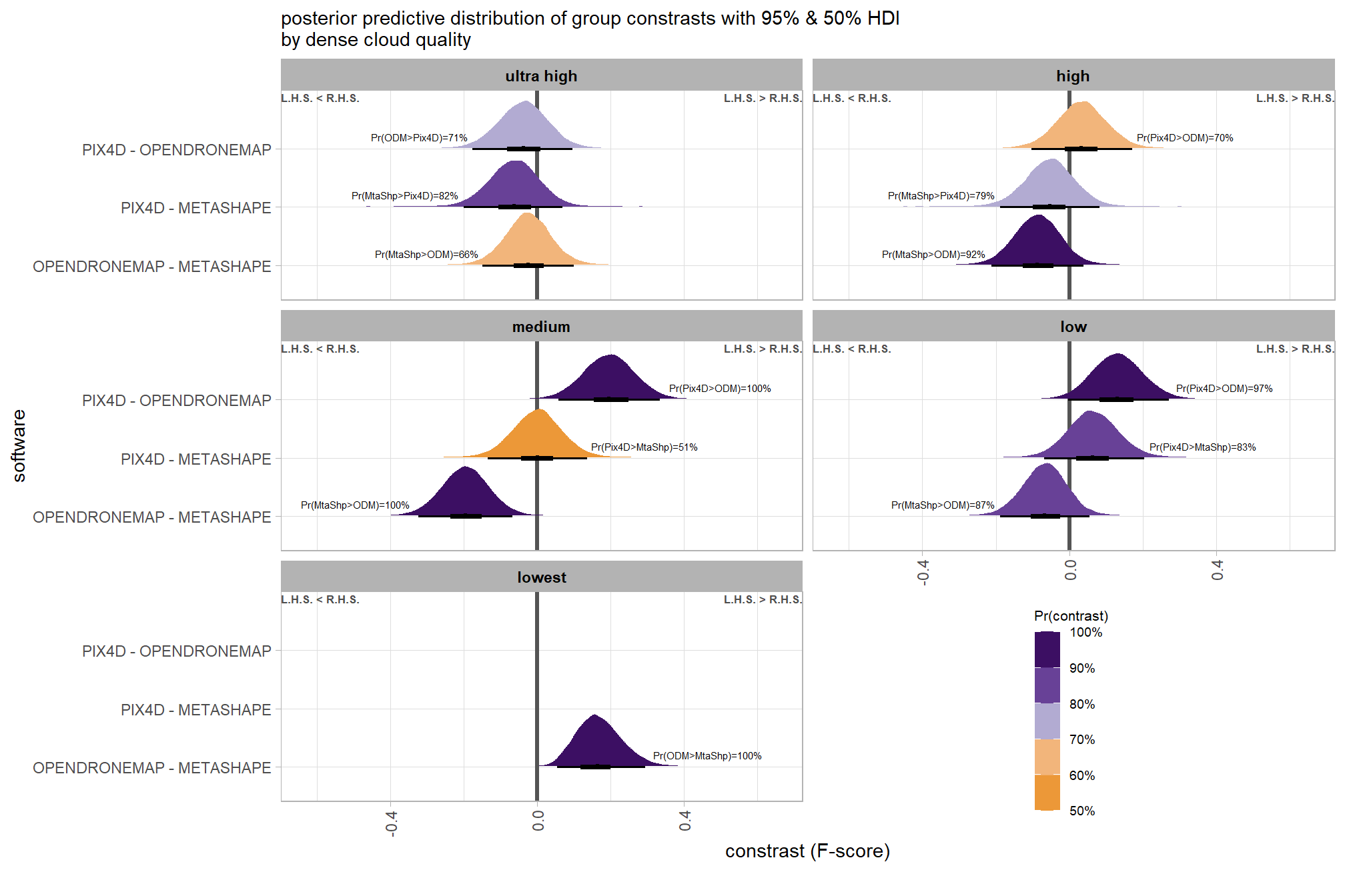
ggplot2::ggsave(
  "../data/sftwr_qlty_comp_mod5.png"
  , plot = ggplot2::last_plot() + labs(subtitle = "")
  , height = 7, width = 10.5
)
create plot for combining with other contrasts for publication
ptchwrk_sftwr_qlty_comp =
  plt_contrast(
    brms_contrast_temp
    , y_axis_title = "software contrast"
    , facet = "depth_maps_generation_quality"
    , label_size = 1.7
    , label = "pr_diff_lab_sm"
    , annotate_size = 1.8
  ) +
    facet_wrap(facets = vars(depth_maps_generation_quality), ncol = 3) +
    labs(
      subtitle = ""
      , x = "F-score constrast"
    ) +
    theme(
      legend.position = "inside"
      , legend.position.inside = c(.8, .11)
      , axis.title.y = element_text(size = 10, face = "bold")
      , axis.title.x = element_text(size = 8)
    ) +
    guides(fill = guide_colorbar(theme = theme(
      legend.key.width  = unit(1, "lines"),
      legend.key.height = unit(7, "lines")
    )))
# ptchwrk_sftwr_qlty_comp
and summarize these contrasts
table_temp = brms_contrast_temp %>%
  dplyr::group_by(contrast, depth_maps_generation_quality, pr_gt_zero) %>%
  tidybayes::median_hdi(value) %>%
  dplyr::arrange(contrast, depth_maps_generation_quality) %>%
  dplyr::select(contrast, depth_maps_generation_quality, value, .lower, .upper, pr_gt_zero)

table_temp %>%
  dplyr::select(-c(contrast)) %>%
  kableExtra::kbl(
    digits = 2
    , caption = "brms::brm model: 95% HDI of the posterior predictive distribution of group constrasts"
    , col.names = c(
      "quality"
      , "median difference<br>F-score"
      , "HDI low", "HDI high"
      , "Pr(diff>0)"
    )
    , escape = F
  ) %>%
  kableExtra::kable_styling() %>%
  kableExtra::pack_rows(index = table(forcats::fct_inorder(table_temp$contrast))) %>%
kableExtra::scroll_box(height = "8in")| quality |
median difference F-score |
HDI low | HDI high | Pr(diff>0) |
|---|---|---|---|---|
| OPENDRONEMAP - METASHAPE | ||||
| ultra high | -0.02 | -0.15 | 0.10 | 34% |
| high | -0.09 | -0.21 | 0.04 | 8% |
| medium | -0.20 | -0.32 | -0.07 | 0% |
| low | -0.07 | -0.19 | 0.06 | 13% |
| lowest | 0.17 | 0.05 | 0.29 | 100% |
| PIX4D - METASHAPE | ||||
| ultra high | -0.06 | -0.20 | 0.07 | 18% |
| high | -0.05 | -0.19 | 0.08 | 21% |
| medium | 0.00 | -0.13 | 0.14 | 51% |
| low | 0.06 | -0.07 | 0.20 | 83% |
| PIX4D - OPENDRONEMAP | ||||
| ultra high | -0.04 | -0.18 | 0.10 | 29% |
| high | 0.03 | -0.10 | 0.17 | 70% |
| medium | 0.20 | 0.06 | 0.33 | 100% |
| low | 0.13 | 0.00 | 0.27 | 97% |
6.7.2.6 Software:Filtering - interaction
Are there differences in F-score based on dense point cloud filtering mode within each processing software?
Here, we collapse across the study site and depth map generation quality to compare the combined filtering mode and software effect.
In a hierarchical model structure, we have to make use of the re_formula argument within tidybayes::add_epred_draws
Even though filtering mode had a small effect on the SfM predictive ability when averaging across all softwares, there might still be differences in filtering mode within software when we average across all depth map generation quality settings. Let’s check the difference in F-score by depth map filtering mode and software.
# get draws
fltr_sftwr_draws_temp = ptcld_validation_data %>%
  dplyr::distinct(depth_maps_generation_filtering_mode, software) %>%
  tidybayes::add_epred_draws(
    brms_f_mod5, allow_new_levels = T
    # this part is crucial
    , re_formula = ~ (1 | depth_maps_generation_filtering_mode) +
      (1 | software) +
      (1 | depth_maps_generation_filtering_mode:software)
  ) %>%
  dplyr::rename(value = .epred) %>%
  dplyr::mutate(med = tidybayes::median_hdci(value)$y)

  # plot
fltr_sftwr_draws_temp %>%
  ggplot(
    mapping = aes(
      y = value, x = software
      # , fill = software
      , fill = med
    )
  ) +
  tidybayes::stat_eye(
    point_interval = median_hdi, .width = .95
    , slab_alpha = 0.95
    , interval_color = "black", linewidth = 1
    , point_color = "black", point_fill = "black", point_size = 1
  ) +
  # scale_fill_viridis_d(option = "rocket", begin = 0.3, end = 0.9, drop = F) +
  scale_fill_viridis_c(option = "mako", direction=-1, begin = 0.2, end = 0.8, limits = c(0,1)) +
  scale_y_continuous(limits = c(0,1), breaks = scales::extended_breaks(n=8)) +
  facet_grid(cols = vars(depth_maps_generation_filtering_mode)) +
  labs(
    x = "software", y = "F-score"
    , subtitle = "posterior predictive distribution of F-score with 95% HDI\nby filtering mode"
    # , caption = form_temp
  ) +
  theme_light() +
  theme(
    legend.position = "none"
    , legend.direction  = "horizontal"
    , axis.text.x = element_text(angle = 90, vjust = 0.5, hjust = 1)
    , strip.text = element_text(color = "black", face = "bold")
) 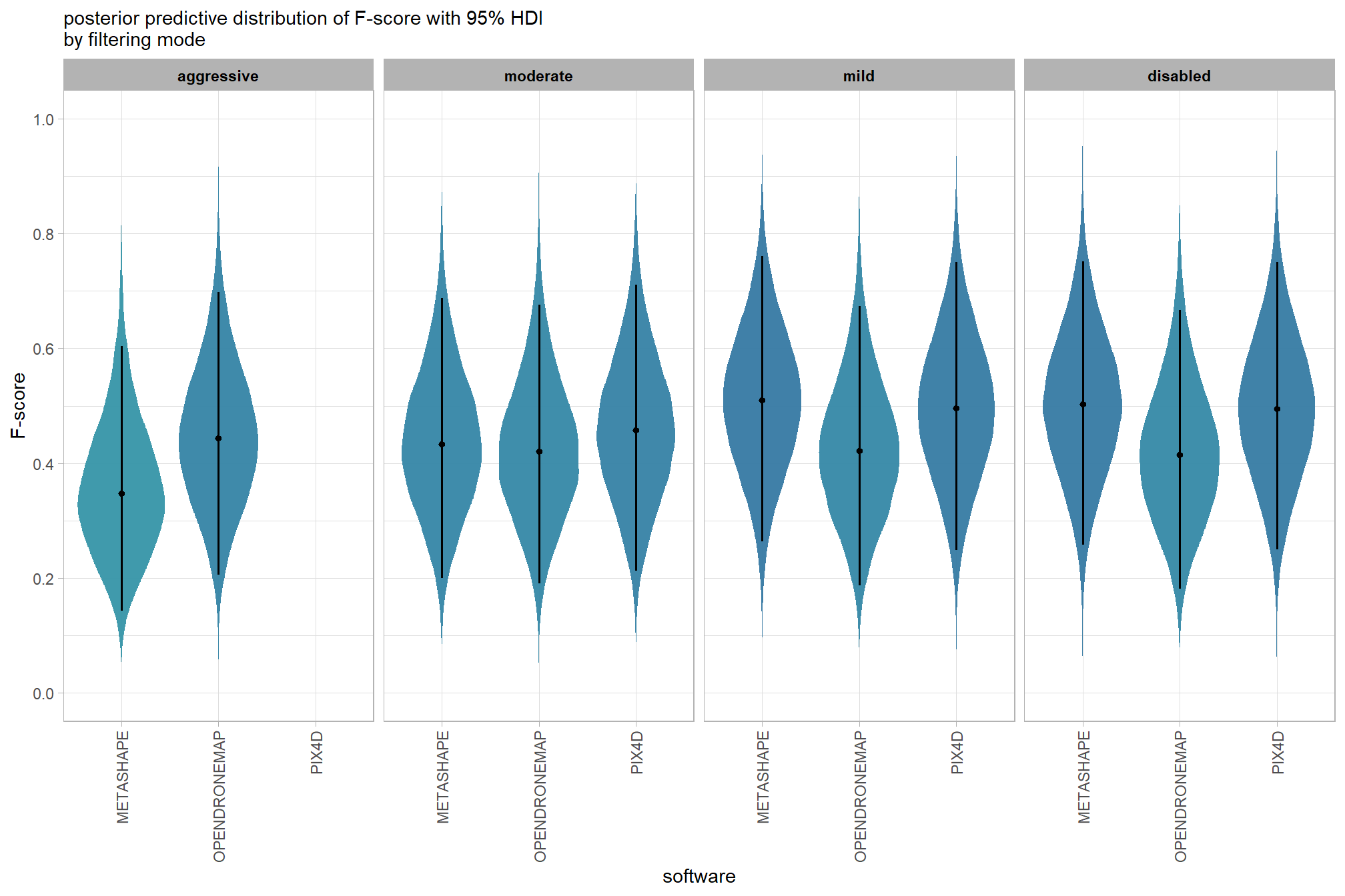
and a table of these 95% HDI values
table_temp =
  fltr_sftwr_draws_temp %>%
    tidybayes::median_hdi(value) %>%
    dplyr::select(-c(.point,.interval, .width,.row)) %>%
    dplyr::arrange(software,depth_maps_generation_filtering_mode)

table_temp %>%
  dplyr::select(-c(software)) %>%
  kableExtra::kbl(
    digits = 2
    , caption = "F-score<br>95% HDI of the posterior predictive distribution"
    , col.names = c(
      "filtering mode"
      , "F-score<br>median"
      , "HDI low", "HDI high"
    )
    , escape = F
  ) %>%
  kableExtra::kable_styling() %>%
  kableExtra::pack_rows(index = table(forcats::fct_inorder(table_temp$software))) %>%
kableExtra::scroll_box(height = "8in")| filtering mode |
F-score median |
HDI low | HDI high |
|---|---|---|---|
| METASHAPE | |||
| aggressive | 0.35 | 0.14 | 0.60 |
| moderate | 0.43 | 0.20 | 0.69 |
| mild | 0.51 | 0.26 | 0.76 |
| disabled | 0.50 | 0.26 | 0.75 |
| OPENDRONEMAP | |||
| aggressive | 0.44 | 0.21 | 0.70 |
| moderate | 0.42 | 0.19 | 0.68 |
| mild | 0.42 | 0.19 | 0.67 |
| disabled | 0.41 | 0.18 | 0.67 |
| PIX4D | |||
| moderate | 0.46 | 0.21 | 0.71 |
| mild | 0.50 | 0.25 | 0.75 |
| disabled | 0.49 | 0.25 | 0.75 |
we can also make pairwise comparisons so long as we continue using tidybayes::add_epred_draws with the re_formula argument
# calculate contrast
brms_contrast_temp = fltr_sftwr_draws_temp %>%
  tidybayes::compare_levels(
    value
    , by = depth_maps_generation_filtering_mode
    , comparison = "pairwise"
  ) %>%
  dplyr::rename(contrast = depth_maps_generation_filtering_mode)

# separate contrast
brms_contrast_temp = brms_contrast_temp %>%
  dplyr::ungroup() %>%
  tidyr::separate_wider_delim(
    cols = contrast
    , delim = " - "
    , names = paste0(
      "sorter"
      , 1:(max(stringr::str_count(brms_contrast_temp$contrast, "-"))+1)
    )
    , too_few = "align_start"
    , cols_remove = F
  ) %>%
  dplyr::filter(sorter1!=sorter2) %>%
  dplyr::mutate(
    dplyr::across(
      tidyselect::starts_with("sorter")
      , .fns = function(x){factor(
        x, ordered = T
        , levels = levels(ptcld_validation_data$depth_maps_generation_filtering_mode)
      )}
    )
    , contrast = contrast %>%
      forcats::fct_reorder(
        paste0(as.numeric(sorter1), as.numeric(sorter2)) %>%
          as.numeric()
      ) %>%
      # re order for filtering mode
      forcats::fct_rev()
  ) %>%
  # median_hdi summary for coloring
  dplyr::group_by(contrast, software) %>%
  make_contrast_vars()

# what?
brms_contrast_temp %>% dplyr::glimpse()
## Rows: 600,000
## Columns: 19
## Groups: contrast, software [15]
## $ software <chr> "METASHAPE", "METASHAPE", "METASHAPE", "METASHAPE", "…
## $ .chain <int> NA, NA, NA, NA, NA, NA, NA, NA, NA, NA, NA, NA, NA, N…
## $ .iteration <int> NA, NA, NA, NA, NA, NA, NA, NA, NA, NA, NA, NA, NA, N…
## $ .draw <int> 1, 2, 3, 4, 5, 6, 7, 8, 9, 10, 11, 12, 13, 14, 15, 16…
## $ sorter1 <ord> moderate, moderate, moderate, moderate, moderate, mod…
## $ sorter2 <ord> aggressive, aggressive, aggressive, aggressive, aggre…
## $ contrast <fct> moderate - aggressive, moderate - aggressive, moderat…
## $ value <dbl> 0.12630997, 0.07866606, 0.08168168, 0.08657663, 0.089…
## $ median_hdi_est <dbl> 0.07955207, 0.07955207, 0.07955207, 0.07955207, 0.079…
## $ median_hdi_lower <dbl> -0.002614075, -0.002614075, -0.002614075, -0.00261407…
## $ median_hdi_upper <dbl> 0.1696683, 0.1696683, 0.1696683, 0.1696683, 0.1696683…
## $ pr_gt_zero <chr> "97%", "97%", "97%", "97%", "97%", "97%", "97%", "97%…
## $ pr_lt_zero <chr> "3%", "3%", "3%", "3%", "3%", "3%", "3%", "3%", "3%",…
## $ is_diff_dir <lgl> TRUE, TRUE, TRUE, TRUE, TRUE, TRUE, TRUE, TRUE, TRUE,…
## $ pr_diff <dbl> 0.973175, 0.973175, 0.973175, 0.973175, 0.973175, 0.9…
## $ pr_diff_lab <chr> "Pr(moderate>aggressive)=97%", "Pr(moderate>aggressiv…
## $ pr_diff_lab_sm <chr> "Pr(>0)=97%", "Pr(>0)=97%", "Pr(>0)=97%", "Pr(>0)=97%…
## $ pr_diff_lab_pos <dbl> 0.1823934, 0.1823934, 0.1823934, 0.1823934, 0.1823934…
## $ sig_level <ord> 95%, 95%, 95%, 95%, 95%, 95%, 95%, 95%, 95%, 95%, 95%…plot it
plt_contrast(
  brms_contrast_temp
  # , caption_text = form_temp
  , y_axis_title = "filtering mode"
  , facet = "software"
  , label_size = 2.0
  , x_expand = c(1.8,1.8) # c(1,1.4)
) +
  labs(
    subtitle = "posterior predictive distribution of group constrasts with 95% & 50% HDI\nby software"
  )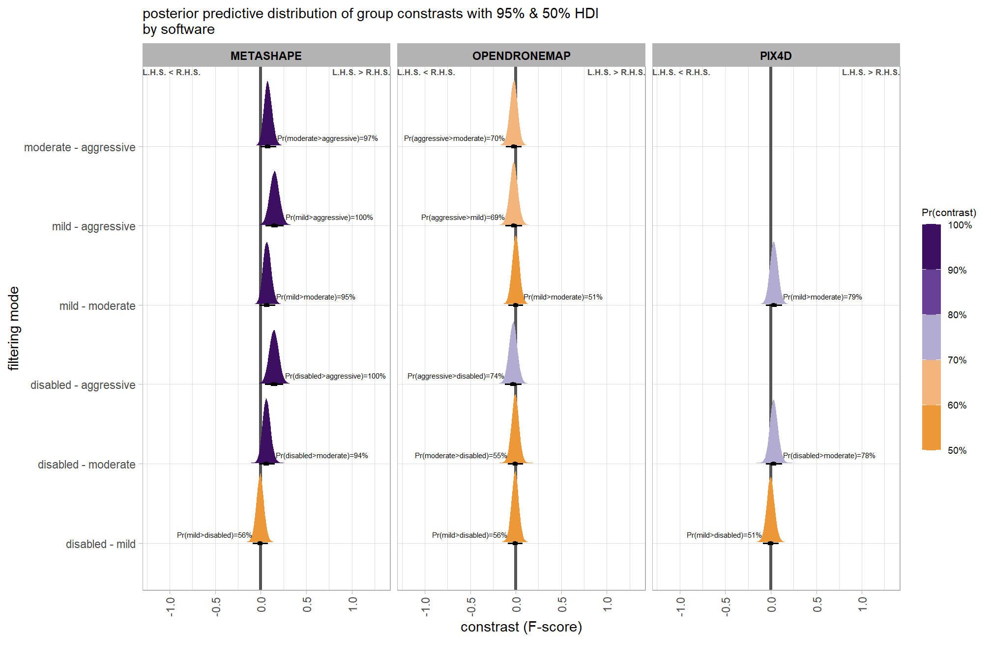
ggplot2::ggsave(
  "../data/fltr_sftwr_comp_mod5.png"
  , plot = ggplot2::last_plot() + labs(subtitle = "")
  , height = 7, width = 10.5
)
create plot for combining with other RMSE contrasts for publication
ptchwrk_fltr_sftwr_comp =
  plt_contrast(
    brms_contrast_temp
    , y_axis_title = "filtering mode contrast"
    , facet = "software"
    , label_size = 1.7
    , label = "pr_diff_lab_sm"
    , annotate_size = 1.8
  ) +
    labs(
      subtitle = "" # "constrast Height RMSE (m)"
      , x = "F-score constrast"
    ) +
    theme(
      legend.position="none"
      , axis.title.y = element_text(size = 10, face = "bold")
      , axis.title.x = element_text(size = 8)
    )
# ptchwrk_fltr_sftwr_comp
and summarize these contrasts
table_temp = brms_contrast_temp %>%
  dplyr::group_by(contrast, software, pr_gt_zero) %>%
  tidybayes::median_hdi(value) %>%
  dplyr::arrange(contrast, software) %>%
  dplyr::select(contrast, software, value, .lower, .upper, pr_gt_zero) %>%
  dplyr::arrange(software, contrast)

table_temp %>%
  dplyr::select(-c(software)) %>%
  kableExtra::kbl(
    digits = 2
    , caption = "brms::brm model: 95% HDI of the posterior predictive distribution of group constrasts"
    , col.names = c(
      "filtering contrast"
      , "median difference<br>F-score"
      , "HDI low", "HDI high"
      , "Pr(diff>0)"
    )
    , escape = F
  ) %>%
  kableExtra::kable_styling() %>%
  kableExtra::pack_rows(index = table(forcats::fct_inorder(table_temp$software))) %>%
kableExtra::scroll_box(height = "8in")| filtering contrast |
median difference F-score |
HDI low | HDI high | Pr(diff>0) |
|---|---|---|---|---|
| METASHAPE | ||||
| disabled - mild | -0.01 | -0.09 | 0.08 | 44% |
| disabled - moderate | 0.06 | -0.02 | 0.15 | 94% |
| disabled - aggressive | 0.15 | 0.05 | 0.25 | 100% |
| mild - moderate | 0.07 | -0.01 | 0.16 | 95% |
| mild - aggressive | 0.15 | 0.05 | 0.25 | 100% |
| moderate - aggressive | 0.08 | 0.00 | 0.17 | 97% |
| OPENDRONEMAP | ||||
| disabled - mild | -0.01 | -0.09 | 0.08 | 44% |
| disabled - moderate | -0.01 | -0.09 | 0.08 | 45% |
| disabled - aggressive | -0.03 | -0.12 | 0.06 | 26% |
| mild - moderate | 0.00 | -0.08 | 0.08 | 51% |
| mild - aggressive | -0.02 | -0.11 | 0.07 | 31% |
| moderate - aggressive | -0.02 | -0.11 | 0.06 | 30% |
| PIX4D | ||||
| disabled - mild | 0.00 | -0.09 | 0.09 | 49% |
| disabled - moderate | 0.03 | -0.05 | 0.12 | 78% |
| mild - moderate | 0.03 | -0.05 | 0.13 | 79% |
6.7.2.7 Software:Quality:Filtering - interaction
The contrasts immediately above address the question “are there differences in F-score based on dense point cloud filtering mode within each software?”. Although the impact of filtering mode is small, it is highly probable when averaging across all quality settings. What if we don’t average out the impact of quality and instead get the full, three-way interaction between software, quality, and filtering mode?
Let’s get the model’s answer to the question “For each software, are there differences in F-score based on dense point cloud filtering mode within each point cloud generation quality?”.
Here, we collapse across the study site to compare the dense cloud quality, filtering mode, and software effect.
In a hierarchical model structure, we have to make use of the re_formula argument within tidybayes::add_epred_draws
# get draws
fltr_sftwr_draws_temp =
  tidyr::crossing(
    depth_maps_generation_quality = unique(ptcld_validation_data$depth_maps_generation_quality)
    , depth_maps_generation_filtering_mode = unique(ptcld_validation_data$depth_maps_generation_filtering_mode)
    , software = unique(ptcld_validation_data$software)
  ) %>%
  tidybayes::add_epred_draws(
    brms_f_mod5, allow_new_levels = T
    # this part is crucial
    , re_formula = ~ (1 | depth_maps_generation_quality) + # main effects
    (1 | depth_maps_generation_quality) +
    (1 | depth_maps_generation_filtering_mode) +
    (1 | software) +
    # two-way interactions
    (1 | depth_maps_generation_quality:depth_maps_generation_filtering_mode) +
    (1 | depth_maps_generation_quality:software) +
    (1 | depth_maps_generation_filtering_mode:software) +
    # three-way interactions
    (1 | depth_maps_generation_quality:depth_maps_generation_filtering_mode:software)
  ) %>%
  dplyr::rename(value = .epred) %>%
  dplyr::mutate(med = tidybayes::median_hdci(value)$y)
# let's add the grand mean to the plot for reference
grand_mean_temp = brms::posterior_summary(brms_f_mod5) %>%
  as.data.frame() %>%
  tibble::rownames_to_column(var = "parameter") %>%
  dplyr::rename_with(tolower) %>%
  dplyr::filter(
    parameter == "Intercept"
  ) %>%
  dplyr::mutate(dplyr::across(-c(parameter), ~plogis(.))) %>%
  dplyr::pull(estimate)
# plot
fltr_sftwr_draws_temp %>%
  dplyr::inner_join(
    ptcld_validation_data %>% dplyr::distinct(software, depth_maps_generation_quality, depth_maps_generation_filtering_mode)
    , by = dplyr::join_by(software, depth_maps_generation_quality, depth_maps_generation_filtering_mode)
  ) %>%
  dplyr::mutate(depth_maps_generation_quality = depth_maps_generation_quality %>% forcats::fct_rev()) %>%
  ggplot(
    mapping = aes(
      y = value
      , x = depth_maps_generation_filtering_mode
      # , fill = depth_maps_generation_filtering_mode
      , fill = med
    )
  ) +
  geom_hline(yintercept = grand_mean_temp, color = "gray33") +
  tidybayes::stat_eye(
    point_interval = median_hdi, .width = .95
    , slab_alpha = 0.95
    , interval_color = "black", linewidth = 1
    , point_color = "black", point_fill = "black", point_size = 1
  ) +
  # scale_fill_viridis_d(option = "plasma", drop = F) +
  scale_fill_viridis_c(option = "mako", direction=-1, begin = 0.2, end = 0.8, limits = c(0,1)) +
  scale_y_continuous(limits = c(0,1), breaks = scales::extended_breaks(n=8)) +
  facet_grid(
    rows = vars(software)
    , cols = vars(depth_maps_generation_quality)
    # , switch = "y"
  ) +
  labs(
    fill = ""
    , x = "filtering mode", y = "F-score"
    # , subtitle = "posterior predictive distribution of F-score with 95% HDI\nby dense cloud quality and software"
    , subtitle = "quality"
    # , caption = form_temp
  ) +
  theme_light() +
  theme(
    legend.position = "none"
    , legend.direction  = "horizontal"
    , axis.text.x = element_text(angle = 90, vjust = 0.5, hjust = 1)
    , strip.text = element_text(color = "black", face = "bold")
    , plot.subtitle = element_text(hjust = 0.5)
    , panel.grid = element_blank()
    # , strip.placement = "outside"
  ) +
  guides(
    fill = guide_legend(override.aes = list(shape = NA, size = 6, alpha = 0.9, lwd = NA))
  )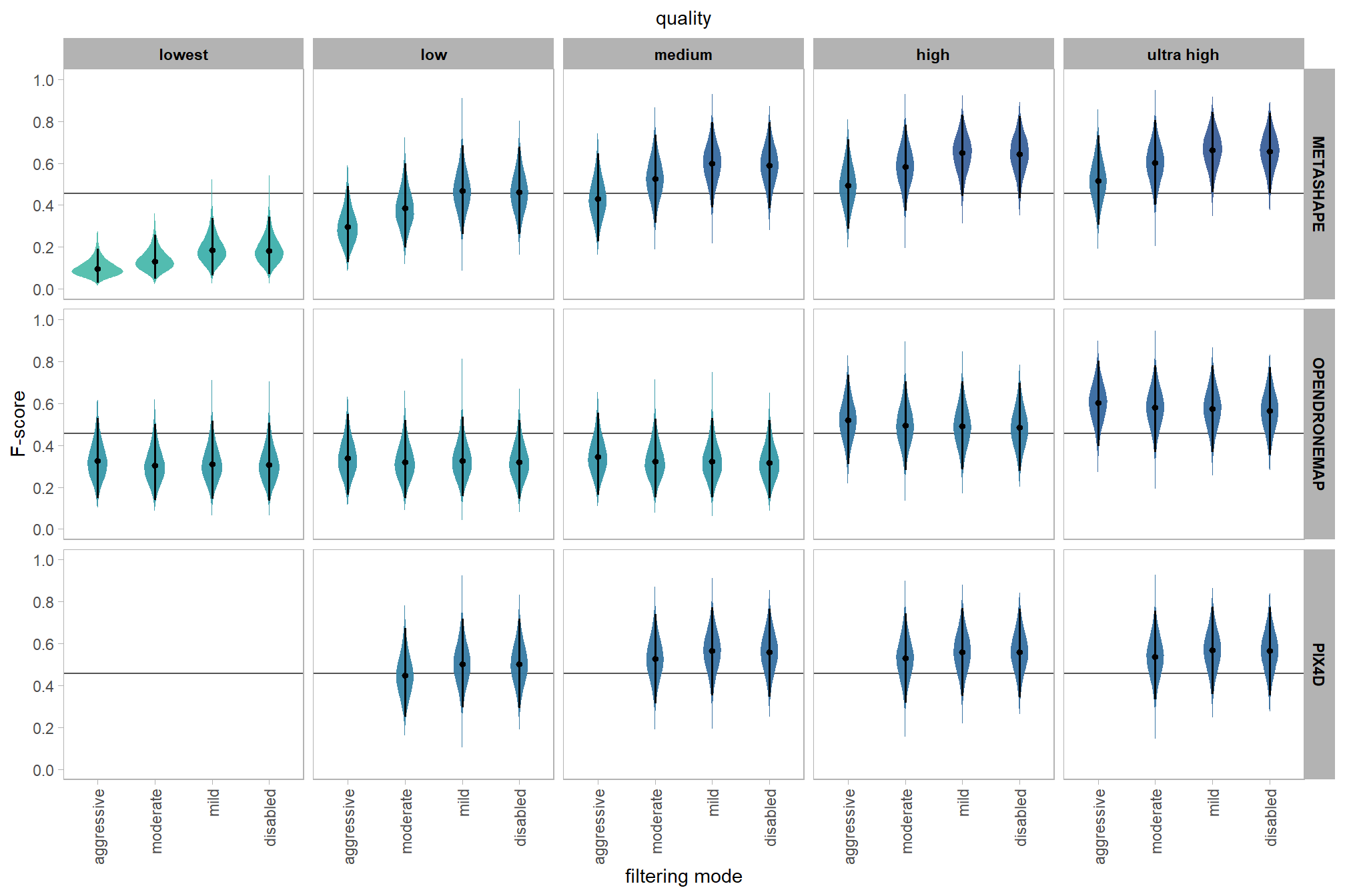
ggplot2::ggsave(
  "../data/qlty_fltr_sftwr_mod5.png"
  , plot = ggplot2::last_plot() + labs(subtitle = "")
  , height = 7, width = 10.5
)
let’s add a table of the results
table_temp =
  fltr_sftwr_draws_temp %>%
  tidybayes::median_hdi(value) %>%
  dplyr::inner_join(
    ptcld_validation_data %>% dplyr::distinct(software, depth_maps_generation_quality, depth_maps_generation_filtering_mode)
    , by = dplyr::join_by(software, depth_maps_generation_quality, depth_maps_generation_filtering_mode)
  ) %>%
  dplyr::mutate(depth_maps_generation_quality = depth_maps_generation_quality %>% forcats::fct_rev()) %>%
  dplyr::select(c(
    software, depth_maps_generation_quality, depth_maps_generation_filtering_mode
    , value, .lower, .upper
  )) %>%
  dplyr::ungroup() %>%
  dplyr::arrange(software, depth_maps_generation_quality, depth_maps_generation_filtering_mode)

table_temp %>%
  # dplyr::select(-c(software)) %>%
  kableExtra::kbl(
    digits = 2
    , caption = "brms::brm model: 95% HDI of the posterior predictive distribution"
    , col.names = c(
      "software", "quality", "filtering mode"
      , "F-score<br>median"
      , "HDI low", "HDI high"
    )
    , escape = F
  ) %>%
  kableExtra::kable_styling() %>%
  # kableExtra::pack_rows(index = table(forcats::fct_inorder(table_temp$software))) %>%
  kableExtra::collapse_rows(columns = 1:2, valign = "top") %>%
kableExtra::scroll_box(height = "8in")| software | quality | filtering mode |
F-score median |
HDI low | HDI high |
|---|---|---|---|---|---|
| METASHAPE | lowest | aggressive | 0.09 | 0.03 | 0.19 |
| moderate | 0.13 | 0.05 | 0.26 | ||
| mild | 0.18 | 0.06 | 0.34 | ||
| disabled | 0.18 | 0.07 | 0.34 | ||
| low | aggressive | 0.30 | 0.13 | 0.49 | |
| moderate | 0.38 | 0.20 | 0.60 | ||
| mild | 0.47 | 0.26 | 0.68 | ||
| disabled | 0.46 | 0.26 | 0.68 | ||
| medium | aggressive | 0.43 | 0.23 | 0.65 | |
| moderate | 0.53 | 0.31 | 0.74 | ||
| mild | 0.60 | 0.39 | 0.80 | ||
| disabled | 0.59 | 0.39 | 0.80 | ||
| high | aggressive | 0.49 | 0.29 | 0.71 | |
| moderate | 0.58 | 0.37 | 0.78 | ||
| mild | 0.65 | 0.44 | 0.83 | ||
| disabled | 0.64 | 0.43 | 0.82 | ||
| ultra high | aggressive | 0.51 | 0.31 | 0.73 | |
| moderate | 0.60 | 0.40 | 0.80 | ||
| mild | 0.66 | 0.46 | 0.84 | ||
| disabled | 0.66 | 0.46 | 0.84 | ||
| OPENDRONEMAP | lowest | aggressive | 0.32 | 0.15 | 0.53 |
| moderate | 0.30 | 0.14 | 0.50 | ||
| mild | 0.31 | 0.14 | 0.52 | ||
| disabled | 0.31 | 0.14 | 0.51 | ||
| low | aggressive | 0.34 | 0.16 | 0.55 | |
| moderate | 0.32 | 0.15 | 0.52 | ||
| mild | 0.33 | 0.16 | 0.54 | ||
| disabled | 0.32 | 0.14 | 0.52 | ||
| medium | aggressive | 0.35 | 0.17 | 0.56 | |
| moderate | 0.32 | 0.15 | 0.53 | ||
| mild | 0.32 | 0.15 | 0.53 | ||
| disabled | 0.32 | 0.15 | 0.52 | ||
| high | aggressive | 0.52 | 0.31 | 0.74 | |
| moderate | 0.49 | 0.28 | 0.70 | ||
| mild | 0.49 | 0.28 | 0.70 | ||
| disabled | 0.48 | 0.28 | 0.70 | ||
| ultra high | aggressive | 0.60 | 0.40 | 0.80 | |
| moderate | 0.58 | 0.37 | 0.78 | ||
| mild | 0.58 | 0.37 | 0.78 | ||
| disabled | 0.56 | 0.35 | 0.77 | ||
| PIX4D | low | moderate | 0.45 | 0.25 | 0.67 |
| mild | 0.50 | 0.29 | 0.72 | ||
| disabled | 0.50 | 0.29 | 0.72 | ||
| medium | moderate | 0.53 | 0.32 | 0.74 | |
| mild | 0.56 | 0.35 | 0.77 | ||
| disabled | 0.56 | 0.35 | 0.77 | ||
| high | moderate | 0.53 | 0.32 | 0.74 | |
| mild | 0.56 | 0.35 | 0.77 | ||
| disabled | 0.56 | 0.34 | 0.76 | ||
| ultra high | moderate | 0.54 | 0.33 | 0.76 | |
| mild | 0.57 | 0.36 | 0.78 | ||
| disabled | 0.56 | 0.35 | 0.77 |
we can also make pairwise comparisons so long as we continue using tidybayes::add_epred_draws with the re_formula argument
# calculate contrast
brms_contrast_temp = fltr_sftwr_draws_temp %>%
  tidybayes::compare_levels(
    value
    , by = depth_maps_generation_filtering_mode
    , comparison = "pairwise"
  ) %>%
  dplyr::rename(contrast = depth_maps_generation_filtering_mode)

# separate contrast
brms_contrast_temp = brms_contrast_temp %>%
  dplyr::ungroup() %>%
  tidyr::separate_wider_delim(
    cols = contrast
    , delim = " - "
    , names = paste0(
      "sorter"
      , 1:(max(stringr::str_count(brms_contrast_temp$contrast, "-"))+1)
    )
    , too_few = "align_start"
    , cols_remove = F
  ) %>%
  dplyr::filter(sorter1!=sorter2) %>%
  dplyr::mutate(
    dplyr::across(
      tidyselect::starts_with("sorter")
      , .fns = function(x){factor(
        x, ordered = T
        , levels = levels(ptcld_validation_data$depth_maps_generation_filtering_mode)
      )}
    )
    , contrast = contrast %>%
      forcats::fct_reorder(
        paste0(as.numeric(sorter1), as.numeric(sorter2)) %>%
          as.numeric()
      ) %>%
      # re order for filtering mode
      forcats::fct_rev()
  ) %>%
  # median_hdi summary for coloring
  dplyr::group_by(contrast, software, depth_maps_generation_quality) %>%
  make_contrast_vars()

# remove out-of-sample obs
brms_contrast_temp = brms_contrast_temp %>%
  dplyr::inner_join(
    ptcld_validation_data %>% dplyr::distinct(software, depth_maps_generation_quality, depth_maps_generation_filtering_mode)
    , by = dplyr::join_by(software, depth_maps_generation_quality, sorter1==depth_maps_generation_filtering_mode)
  ) %>%
  dplyr::inner_join(
    ptcld_validation_data %>% dplyr::distinct(software, depth_maps_generation_quality, depth_maps_generation_filtering_mode)
    , by = dplyr::join_by(software, depth_maps_generation_quality, sorter2==depth_maps_generation_filtering_mode)
  ) %>%
  dplyr::mutate(depth_maps_generation_quality = depth_maps_generation_quality %>% forcats::fct_rev())

# what?
brms_contrast_temp %>% dplyr::glimpse()
## Rows: 2,880,000
## Columns: 20
## Groups: contrast, software, depth_maps_generation_quality [72]
## $ depth_maps_generation_quality <ord> ultra high, ultra high, ultra high, ultr…
## $ software <chr> "METASHAPE", "METASHAPE", "METASHAPE", "…
## $ .chain <int> NA, NA, NA, NA, NA, NA, NA, NA, NA, NA, …
## $ .iteration <int> NA, NA, NA, NA, NA, NA, NA, NA, NA, NA, …
## $ .draw <int> 1, 2, 3, 4, 5, 6, 7, 8, 9, 10, 11, 12, 1…
## $ sorter1 <ord> moderate, moderate, moderate, moderate, …
## $ sorter2 <ord> aggressive, aggressive, aggressive, aggr…
## $ contrast <fct> moderate - aggressive, moderate - aggres…
## $ value <dbl> 0.12558985, 0.09105310, 0.08415801, 0.08…
## $ median_hdi_est <dbl> 0.08333826, 0.08333826, 0.08333826, 0.08…
## $ median_hdi_lower <dbl> -0.02002375, -0.02002375, -0.02002375, -…
## $ median_hdi_upper <dbl> 0.1847667, 0.1847667, 0.1847667, 0.18476…
## $ pr_gt_zero <chr> "95%", "95%", "95%", "95%", "95%", "95%"…
## $ pr_lt_zero <chr> "5%", "5%", "5%", "5%", "5%", "5%", "5%"…
## $ is_diff_dir <lgl> TRUE, TRUE, TRUE, TRUE, TRUE, TRUE, TRUE…
## $ pr_diff <dbl> 0.9482, 0.9482, 0.9482, 0.9482, 0.9482, …
## $ pr_diff_lab <chr> "Pr(moderate>aggressive)=95%", "Pr(moder…
## $ pr_diff_lab_sm <chr> "Pr(>0)=95%", "Pr(>0)=95%", "Pr(>0)=95%"…
## $ pr_diff_lab_pos <dbl> 0.1986242, 0.1986242, 0.1986242, 0.19862…
## $ sig_level <ord> 90%, 90%, 90%, 90%, 90%, 90%, 90%, 90%, …plot it
brms_contrast_temp %>%
  plt_contrast(
    facet = c("depth_maps_generation_quality", "software")
    , y_axis_title = "filtering mode"
    , label_size = 0
    , x_expand = c(-0.1,-0.1)
  ) +
  facet_grid(
    rows = vars(software)
    , cols = vars(depth_maps_generation_quality)
  ) +
  labs(
    subtitle = "posterior predictive distribution of group constrasts with 95% & 50% HDI\nby dense cloud quality and software"
  )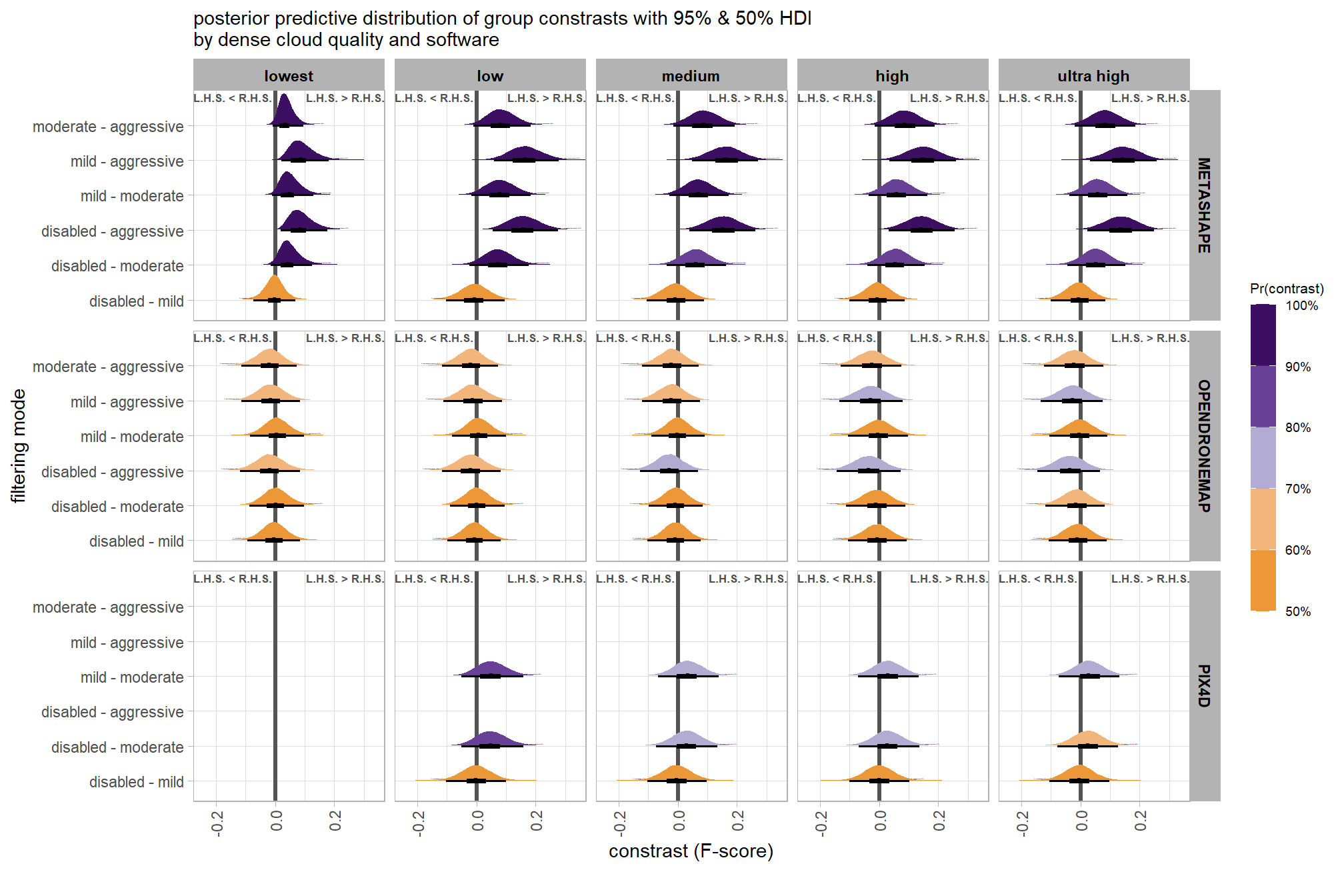
6.7.2.8 Quality - main effect
let’s collapse across the filtering mode, software, and study site to compare the dense cloud quality setting effect.
In a hierarchical model structure, we have to make use of the re_formula argument within tidybayes::add_epred_draws
ptcld_validation_data %>%
  dplyr::distinct(depth_maps_generation_quality) %>%
  tidybayes::add_epred_draws(
    brms_f_mod5
    # this part is crucial
    , re_formula = ~ (1 | depth_maps_generation_quality)
  ) %>%
  dplyr::rename(value = .epred) %>%
  dplyr::mutate(med = tidybayes::median_hdci(value)$y) %>%
  # plot
  ggplot(
    mapping = aes(
      x = value, y = depth_maps_generation_quality
      # , fill = depth_maps_generation_quality
      , fill = med
    )
  ) +
    tidybayes::stat_halfeye(
      point_interval = median_hdi, .width = .95
      , interval_color = "gray66"
      , shape = 21, point_color = "gray66", point_fill = "black"
      , justification = -0.01
    ) +
    # scale_fill_viridis_d(option = "inferno", drop = F) +
    scale_fill_viridis_c(option = "mako", direction=-1, begin = 0.2, end = 0.8, limits = c(0,1)) +
    scale_x_continuous(limits = c(0,1), breaks = scales::extended_breaks(n=8)) +
    # scale_x_continuous(breaks = scales::extended_breaks(n=8)) +
    labs(
      y = "quality", x = "F-score"
      , subtitle = "posterior predictive distribution of F-score with 95% HDI"
      # , caption = form_temp
    ) +
    theme_light() +
    theme(legend.position = "none")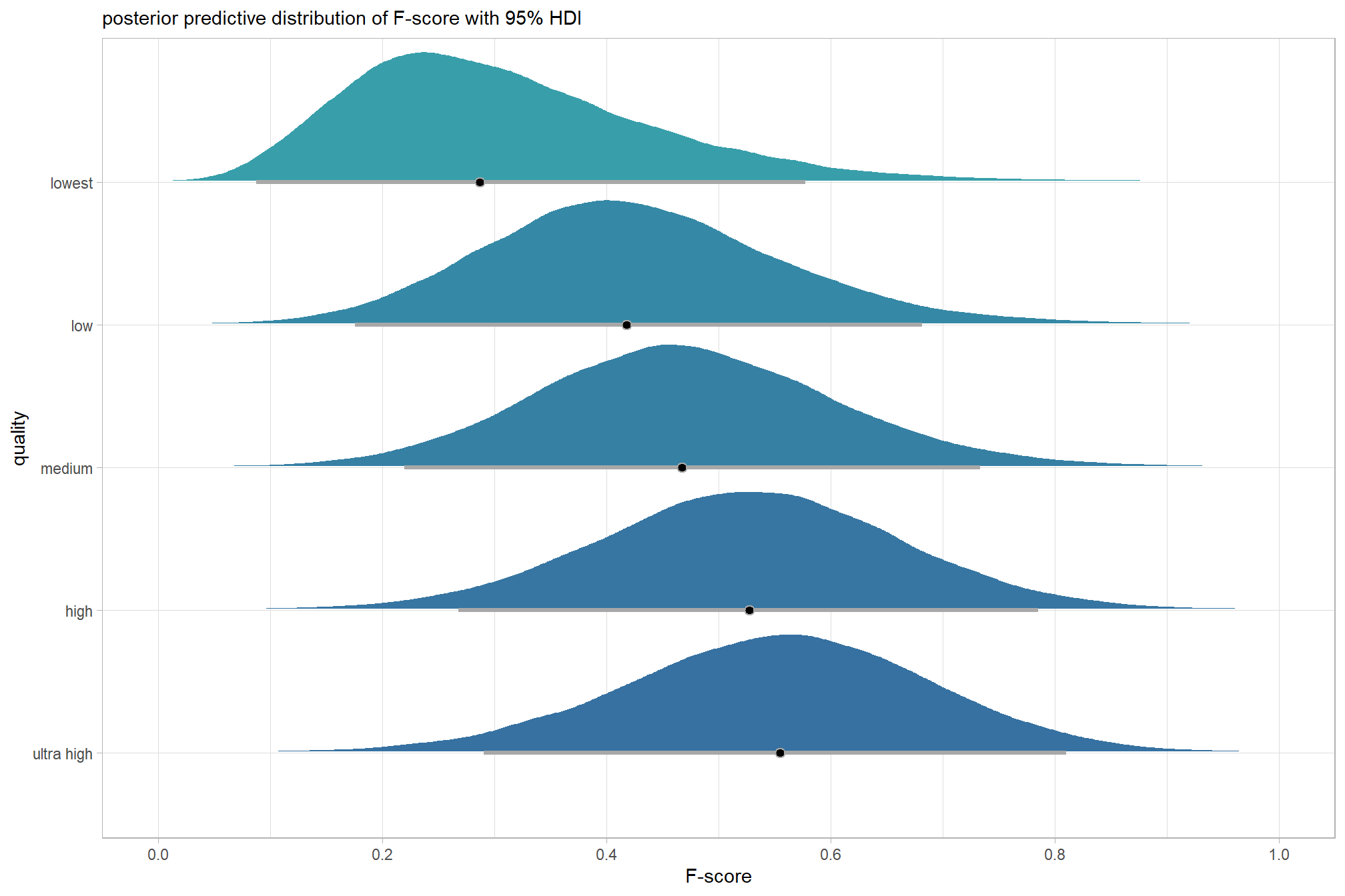
let’s compare these results to the results from our one nominal predictor model above, two nominal predictor model above, three nominal predictor model above, and three nominal predictor + site effects model above
ptcld_validation_data %>%
  dplyr::distinct(depth_maps_generation_quality) %>%
  tidybayes::add_epred_draws(
    brms_f_mod5
    # this part is crucial
    , re_formula = ~ (1 | depth_maps_generation_quality)
  ) %>%
  dplyr::mutate(value = .epred, src = "brms_f_mod5") %>%
  dplyr::bind_rows(
    ptcld_validation_data %>%
      dplyr::distinct(depth_maps_generation_quality) %>%
      tidybayes::add_epred_draws(
        brms_f_mod4
        # this part is crucial
        , re_formula = ~ (1 | depth_maps_generation_quality)
      ) %>%
      dplyr::mutate(value = .epred, src = "brms_f_mod4")
    , ptcld_validation_data %>%
      dplyr::distinct(depth_maps_generation_quality) %>%
      tidybayes::add_epred_draws(
        brms_f_mod3
        # this part is crucial
        , re_formula = ~ (1 | depth_maps_generation_quality)
      ) %>%
      dplyr::mutate(value = .epred, src = "brms_f_mod3")
    , ptcld_validation_data %>%
      dplyr::distinct(depth_maps_generation_quality) %>%
      tidybayes::add_epred_draws(
        brms_f_mod2
        # this part is crucial
        , re_formula = ~ (1 | depth_maps_generation_quality)
      ) %>%
      dplyr::mutate(value = .epred, src = "brms_f_mod2")
    , ptcld_validation_data %>%
      dplyr::distinct(depth_maps_generation_quality) %>%
      tidybayes::add_epred_draws(brms_f_mod1) %>%
      dplyr::mutate(value = .epred, src = "brms_f_mod1")
  ) %>%
  ggplot(mapping = aes(y = src, x = value, color = src, group = src)) +
  tidybayes::stat_pointinterval(position = "dodge") +
  facet_grid(rows = vars(depth_maps_generation_quality), switch = "y") +
  scale_y_discrete(NULL, breaks = NULL) +
  # scale_color_viridis_d(option = "turbo", begin = 0.2, end = 0.8) +
  scale_color_manual(values = viridis::turbo(n = 6, begin = 0.2, end = 0.8)) +
  labs(
    y = "", x = "F-score"
    , color = "model"
  ) +
  theme_light() +
  theme(legend.position = "top", strip.text = element_text(color = "black", face = "bold"))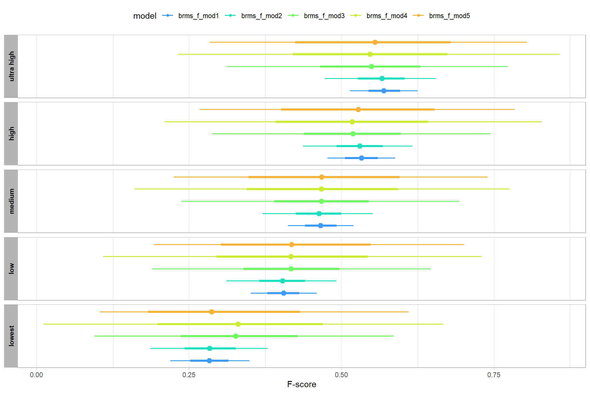
we can also perform pairwise comparisons after collapsing across the filtering mode, software, and study site to compare the dense cloud quality setting effect
brms_contrast_temp =
  ptcld_validation_data %>%
    dplyr::distinct(depth_maps_generation_quality) %>%
    tidybayes::add_epred_draws(
      brms_f_mod5, allow_new_levels = T
      # this part is crucial
      , re_formula = ~ (1 | depth_maps_generation_quality)
    ) %>%
    dplyr::rename(value = .epred) %>%
    tidybayes::compare_levels(
      value
      , by = depth_maps_generation_quality
      , comparison =
        contrast_list
        # tidybayes::emmeans_comparison("revpairwise")
        #"pairwise"
    ) %>%
    dplyr::rename(contrast = depth_maps_generation_quality)

# separate contrast
brms_contrast_temp = brms_contrast_temp %>%
  dplyr::ungroup() %>%
  tidyr::separate_wider_delim(
    cols = contrast
    , delim = " - "
    , names = paste0(
        "sorter"
        , 1:(max(stringr::str_count(brms_contrast_temp$contrast, "-"))+1)
      )
    , too_few = "align_start"
    , cols_remove = F
  ) %>%
  dplyr::filter(sorter1!=sorter2) %>%
  dplyr::mutate(
    dplyr::across(
      tidyselect::starts_with("sorter")
      , .fns = function(x){factor(
        x, ordered = T
        , levels = levels(ptcld_validation_data$depth_maps_generation_quality)
      )}
    )
    , contrast = contrast %>%
      forcats::fct_reorder(
        paste0(as.numeric(sorter1), as.numeric(sorter2)) %>%
        as.numeric()
      )
  ) %>%
  # median_hdi summary for coloring
  dplyr::group_by(contrast) %>%
  make_contrast_vars()

# what?
brms_contrast_temp %>% dplyr::glimpse()
## Rows: 400,000
## Columns: 18
## Groups: contrast [10]
## $ .chain <int> NA, NA, NA, NA, NA, NA, NA, NA, NA, NA, NA, NA, NA, N…
## $ .iteration <int> NA, NA, NA, NA, NA, NA, NA, NA, NA, NA, NA, NA, NA, N…
## $ .draw <int> 1, 2, 3, 4, 5, 6, 7, 8, 9, 10, 11, 12, 13, 14, 15, 16…
## $ sorter1 <ord> ultra high, ultra high, ultra high, ultra high, ultra…
## $ sorter2 <ord> high, high, high, high, high, high, high, high, high,…
## $ contrast <fct> ultra high - high, ultra high - high, ultra high - hi…
## $ value <dbl> -0.037051693, 0.077710938, 0.032518207, 0.021371253, …
## $ median_hdi_est <dbl> 0.02227479, 0.02227479, 0.02227479, 0.02227479, 0.022…
## $ median_hdi_lower <dbl> -0.1425197, -0.1425197, -0.1425197, -0.1425197, -0.14…
## $ median_hdi_upper <dbl> 0.1992295, 0.1992295, 0.1992295, 0.1992295, 0.1992295…
## $ pr_gt_zero <chr> "62%", "62%", "62%", "62%", "62%", "62%", "62%", "62%…
## $ pr_lt_zero <chr> "38%", "38%", "38%", "38%", "38%", "38%", "38%", "38%…
## $ is_diff_dir <lgl> FALSE, TRUE, TRUE, TRUE, TRUE, TRUE, TRUE, TRUE, FALS…
## $ pr_diff <dbl> 0.621175, 0.621175, 0.621175, 0.621175, 0.621175, 0.6…
## $ pr_diff_lab <chr> "Pr(ultra high>high)=62%", "Pr(ultra high>high)=62%",…
## $ pr_diff_lab_sm <chr> "Pr(>0)=62%", "Pr(>0)=62%", "Pr(>0)=62%", "Pr(>0)=62%…
## $ pr_diff_lab_pos <dbl> 0.2141717, 0.2141717, 0.2141717, 0.2141717, 0.2141717…
## $ sig_level <ord> <80%, <80%, <80%, <80%, <80%, <80%, <80%, <80%, <80%,…plot it
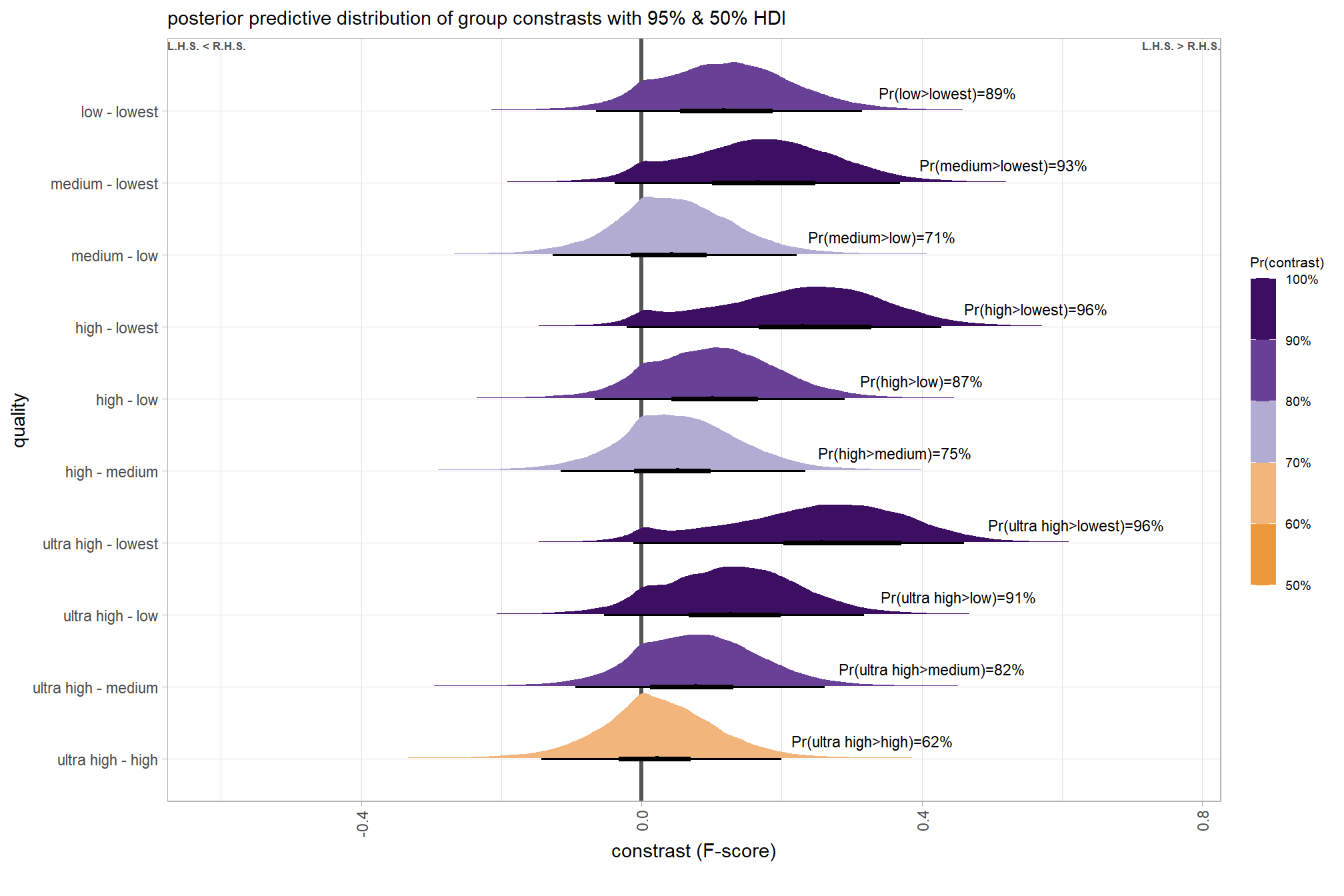
and summarize these contrasts
brms_contrast_temp %>%
  dplyr::group_by(contrast, pr_gt_zero) %>%
  tidybayes::median_hdi(value) %>%
  dplyr::arrange(contrast) %>%
  dplyr::select(contrast, value, .lower, .upper, pr_gt_zero) %>%

kableExtra::kbl(
    digits = 2
    , caption = "brms::brm model: 95% HDI of the posterior predictive distribution of group constrasts"
    , col.names = c(
      "quality contrast"
      , "difference (F-score)"
      , "HDI low", "HDI high"
      , "Pr(diff>0)"
    )
  ) %>%
kableExtra::kable_styling()| quality contrast | difference (F-score) | HDI low | HDI high | Pr(diff>0) |
|---|---|---|---|---|
| ultra high - high | 0.02 | -0.14 | 0.20 | 62% |
| ultra high - medium | 0.08 | -0.09 | 0.26 | 82% |
| ultra high - low | 0.13 | -0.05 | 0.32 | 91% |
| ultra high - lowest | 0.26 | -0.01 | 0.46 | 96% |
| high - medium | 0.05 | -0.12 | 0.23 | 75% |
| high - low | 0.10 | -0.07 | 0.29 | 87% |
| high - lowest | 0.23 | -0.02 | 0.43 | 96% |
| medium - low | 0.04 | -0.13 | 0.22 | 71% |
| medium - lowest | 0.17 | -0.04 | 0.37 | 93% |
| low - lowest | 0.12 | -0.06 | 0.31 | 89% |
6.7.2.9 Filtering - main effect
let’s collapse across the dense cloud quality, software, and study site to compare the dense cloud quality setting effect.
In a hierarchical model structure, we have to make use of the re_formula argument within tidybayes::add_epred_draws
ptcld_validation_data %>%
  dplyr::distinct(depth_maps_generation_filtering_mode) %>%
  tidybayes::add_epred_draws(
    brms_f_mod5
    # this part is crucial
    , re_formula = ~ (1 | depth_maps_generation_filtering_mode)
  ) %>%
  dplyr::rename(value = .epred) %>%
  dplyr::mutate(med = tidybayes::median_hdci(value)$y) %>%
  # plot
  ggplot(
    mapping = aes(
      x = value, y = depth_maps_generation_filtering_mode
      # , fill = depth_maps_generation_filtering_mode
      , fill = med
    )
  ) +
    tidybayes::stat_halfeye(
      point_interval = median_hdi, .width = .95
      , interval_color = "gray66"
      , shape = 21, point_color = "gray66", point_fill = "black"
      , justification = -0.01
    ) +
    # scale_fill_viridis_d(option = "plasma", drop = F) +
    scale_fill_viridis_c(option = "mako", direction=-1, begin = 0.2, end = 0.8, limits = c(0,1)) +
    scale_x_continuous(limits = c(0,1), breaks = scales::extended_breaks(n=8)) +
    labs(
      y = "filtering mode", x = "F-score"
      , subtitle = "posterior predictive distribution of F-score with 95% HDI"
      # , caption = form_temp
    ) +
    theme_light() +
    theme(legend.position = "none")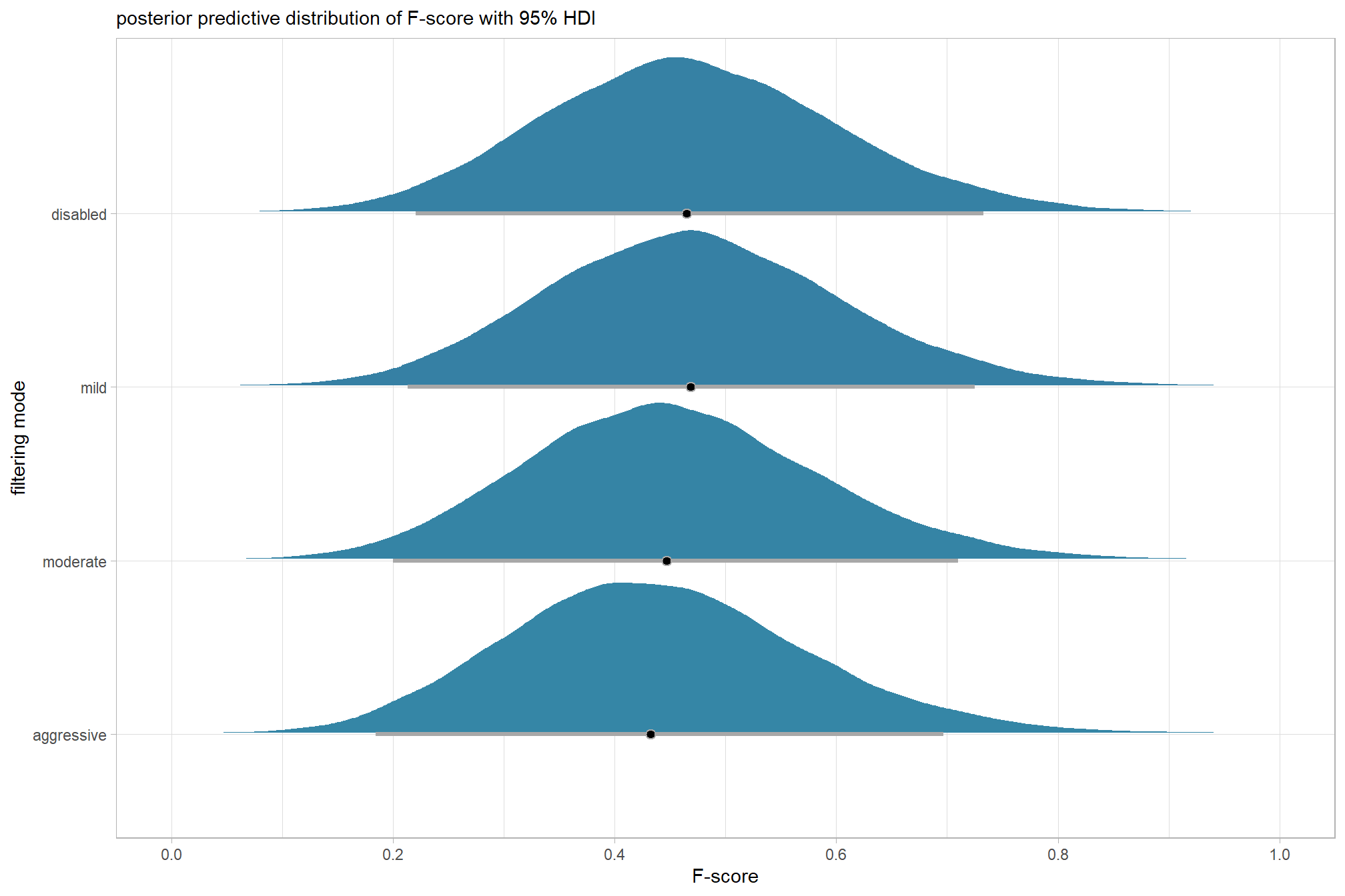
let’s compare these results to the results from our two nominal predictor model above, three nominal predictor model above, and three nominal predictor + site model above
ptcld_validation_data %>%
  dplyr::distinct(depth_maps_generation_filtering_mode) %>%
  tidybayes::add_epred_draws(
    brms_f_mod5
    # this part is crucial
    , re_formula = ~ (1 | depth_maps_generation_filtering_mode)
  ) %>%
  dplyr::mutate(value = .epred, src = "brms_f_mod5") %>%
  dplyr::bind_rows(
    ptcld_validation_data %>%
      dplyr::distinct(depth_maps_generation_filtering_mode) %>%
      tidybayes::add_epred_draws(
        brms_f_mod4
        # this part is crucial
        , re_formula = ~ (1 | depth_maps_generation_filtering_mode)
      ) %>%
      dplyr::mutate(value = .epred, src = "brms_f_mod4")
    , ptcld_validation_data %>%
      dplyr::distinct(depth_maps_generation_filtering_mode) %>%
      tidybayes::add_epred_draws(
        brms_f_mod3
        # this part is crucial
        , re_formula = ~ (1 | depth_maps_generation_filtering_mode)
      ) %>%
      dplyr::mutate(value = .epred, src = "brms_f_mod3")
    , ptcld_validation_data %>%
      dplyr::distinct(depth_maps_generation_filtering_mode) %>%
      tidybayes::add_epred_draws(
        brms_f_mod2
        # this part is crucial
        , re_formula = ~ (1 | depth_maps_generation_filtering_mode)
      ) %>%
      dplyr::mutate(value = .epred, src = "brms_f_mod2")
  ) %>%
  ggplot(mapping = aes(y = src, x = value, color = src, group = src)) +
  tidybayes::stat_pointinterval(position = "dodge") +
  facet_grid(rows = vars(depth_maps_generation_filtering_mode), switch = "y") +
  scale_y_discrete(NULL, breaks = NULL) +
  scale_color_manual(values = viridis::turbo(n = 6, begin = 0.2, end = 0.8)[2:5]) +
  labs(
    y = "filtering mode", x = "F-score"
    , color = "model"
  ) +
  theme_light() +
  theme(legend.position = "top", strip.text = element_text(color = "black", face = "bold"))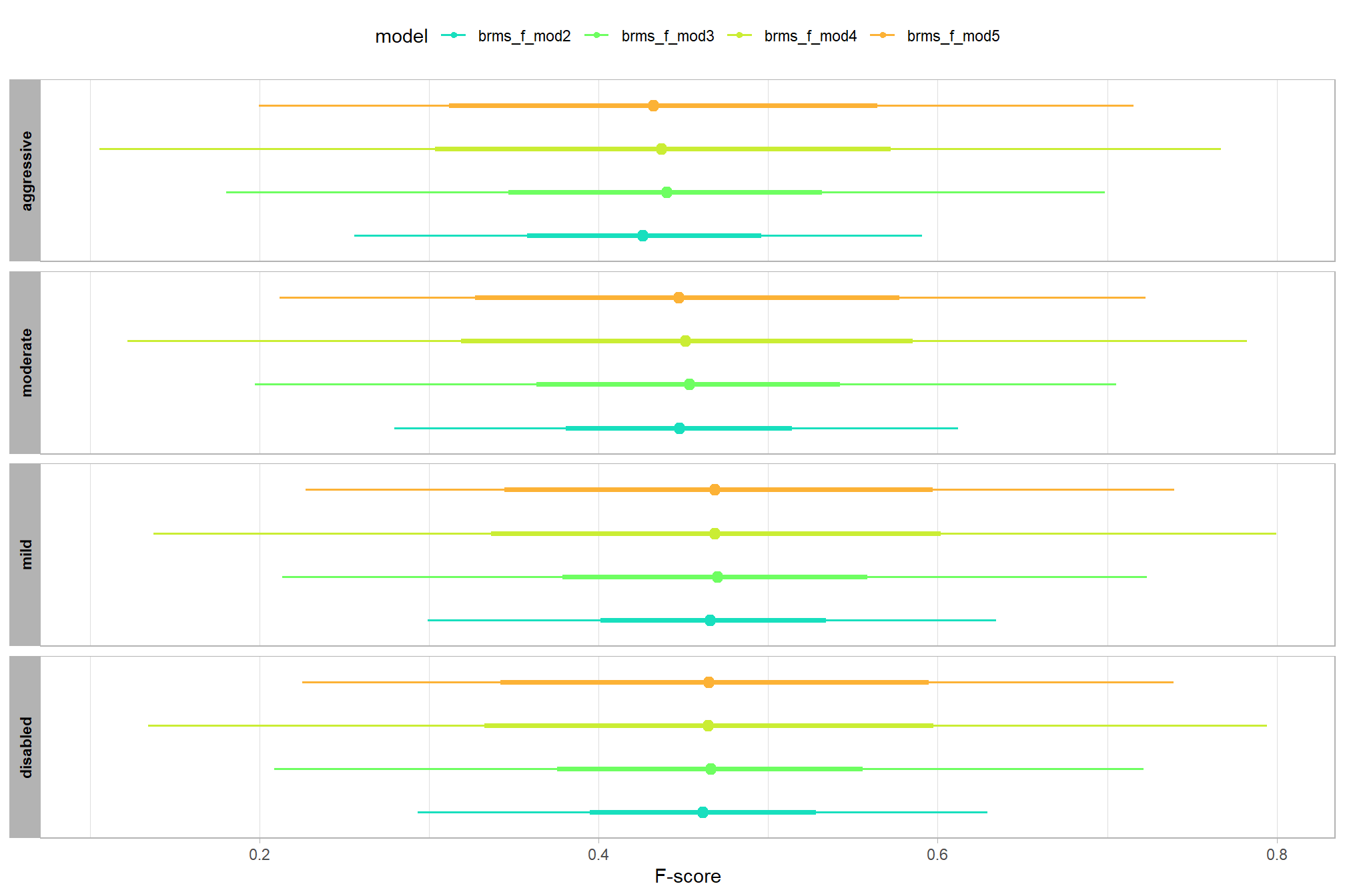
we can also perform pairwise comparisons after collapsing across the dense cloud quality, software, and study site to compare the filtering mode setting effect.
brms_contrast_temp =
  ptcld_validation_data %>%
    dplyr::distinct(depth_maps_generation_filtering_mode) %>%
    tidybayes::add_epred_draws(
      brms_f_mod5, allow_new_levels = T
      # this part is crucial
      , re_formula = ~ (1 | depth_maps_generation_filtering_mode)
    ) %>%
    dplyr::rename(value = .epred) %>%
    tidybayes::compare_levels(
      value
      , by = depth_maps_generation_filtering_mode
      , comparison = "pairwise"
    ) %>%
    dplyr::rename(contrast = depth_maps_generation_filtering_mode)

# separate contrast
brms_contrast_temp = brms_contrast_temp %>%
  dplyr::ungroup() %>%
  tidyr::separate_wider_delim(
    cols = contrast
    , delim = " - "
    , names = paste0(
        "sorter"
        , 1:(max(stringr::str_count(brms_contrast_temp$contrast, "-"))+1)
      )
    , too_few = "align_start"
    , cols_remove = F
  ) %>%
  dplyr::filter(sorter1!=sorter2) %>%
  dplyr::mutate(
    dplyr::across(
      tidyselect::starts_with("sorter")
      , .fns = function(x){factor(
        x, ordered = T
        , levels = levels(ptcld_validation_data$depth_maps_generation_filtering_mode)
      )}
    )
    , contrast = contrast %>%
      forcats::fct_reorder(
        paste0(as.numeric(sorter1), as.numeric(sorter2)) %>%
        as.numeric()
      ) %>%
      # re order for filtering mode
      forcats::fct_rev()
  ) %>%
  # median_hdi summary for coloring
  dplyr::group_by(contrast) %>%
  make_contrast_vars()

# what?
brms_contrast_temp %>% dplyr::glimpse()
## Rows: 240,000
## Columns: 18
## Groups: contrast [6]
## $ .chain <int> NA, NA, NA, NA, NA, NA, NA, NA, NA, NA, NA, NA, NA, N…
## $ .iteration <int> NA, NA, NA, NA, NA, NA, NA, NA, NA, NA, NA, NA, NA, N…
## $ .draw <int> 1, 2, 3, 4, 5, 6, 7, 8, 9, 10, 11, 12, 13, 14, 15, 16…
## $ sorter1 <ord> moderate, moderate, moderate, moderate, moderate, mod…
## $ sorter2 <ord> aggressive, aggressive, aggressive, aggressive, aggre…
## $ contrast <fct> moderate - aggressive, moderate - aggressive, moderat…
## $ value <dbl> -0.021519265, -0.038456122, 0.005716817, 0.043144326,…
## $ median_hdi_est <dbl> 0.006865148, 0.006865148, 0.006865148, 0.006865148, 0…
## $ median_hdi_lower <dbl> -0.07420937, -0.07420937, -0.07420937, -0.07420937, -…
## $ median_hdi_upper <dbl> 0.1128279, 0.1128279, 0.1128279, 0.1128279, 0.1128279…
## $ pr_gt_zero <chr> "62%", "62%", "62%", "62%", "62%", "62%", "62%", "62%…
## $ pr_lt_zero <chr> "38%", "38%", "38%", "38%", "38%", "38%", "38%", "38%…
## $ is_diff_dir <lgl> FALSE, FALSE, TRUE, TRUE, TRUE, FALSE, TRUE, FALSE, F…
## $ pr_diff <dbl> 0.618725, 0.618725, 0.618725, 0.618725, 0.618725, 0.6…
## $ pr_diff_lab <chr> "Pr(moderate>aggressive)=62%", "Pr(moderate>aggressiv…
## $ pr_diff_lab_sm <chr> "Pr(>0)=62%", "Pr(>0)=62%", "Pr(>0)=62%", "Pr(>0)=62%…
## $ pr_diff_lab_pos <dbl> 0.1212899, 0.1212899, 0.1212899, 0.1212899, 0.1212899…
## $ sig_level <ord> <80%, <80%, <80%, <80%, <80%, <80%, <80%, <80%, <80%,…plot it
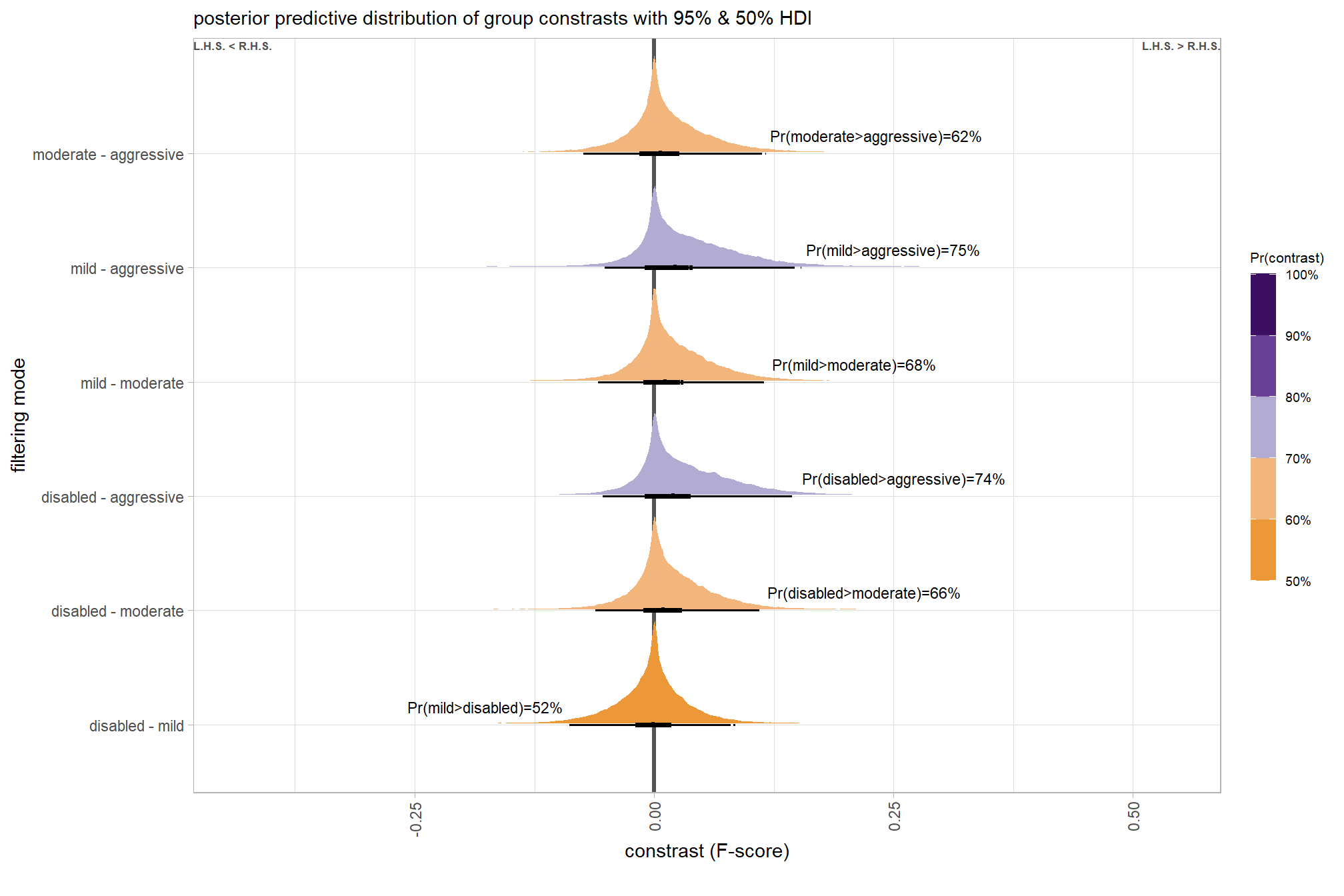
and summarize these contrasts
brms_contrast_temp %>%
  dplyr::group_by(contrast, pr_gt_zero) %>%
  tidybayes::median_hdi(value) %>%
  dplyr::arrange(contrast) %>%
  dplyr::select(contrast, value, .lower, .upper, pr_gt_zero) %>%

kableExtra::kbl(
    digits = 2
    , caption = "brms::brm model: 95% HDI of the posterior predictive distribution of group constrasts"
    , col.names = c(
      "filtering mode contrast"
      , "difference (F-score)"
      , "HDI low", "HDI high"
      , "Pr(diff>0)"
    )
  ) %>%
kableExtra::kable_styling()| filtering mode contrast | difference (F-score) | HDI low | HDI high | Pr(diff>0) |
|---|---|---|---|---|
| disabled - mild | 0.00 | -0.09 | 0.08 | 48% |
| disabled - mild | 0.00 | 0.08 | 0.08 | 48% |
| disabled - moderate | 0.01 | -0.06 | 0.11 | 66% |
| disabled - aggressive | 0.02 | -0.05 | 0.14 | 74% |
| disabled - aggressive | 0.02 | 0.15 | 0.15 | 74% |
| mild - moderate | 0.01 | -0.06 | 0.11 | 68% |
| mild - aggressive | 0.02 | -0.05 | 0.15 | 75% |
| mild - aggressive | 0.02 | 0.15 | 0.15 | 75% |
| moderate - aggressive | 0.01 | -0.07 | 0.11 | 62% |
| moderate - aggressive | 0.01 | 0.12 | 0.12 | 62% |
6.7.2.10 Software - main effect
to address one of our main questions, let’s also collapse across the study site, dense cloud quality, and filtering mode setting to compare the software effect.
In a hierarchical model structure, we have to make use of the re_formula argument within tidybayes::add_epred_draws
ptcld_validation_data %>%
  dplyr::distinct(software) %>%
  tidybayes::add_epred_draws(
    brms_f_mod5
    # this part is crucial
    , re_formula = ~ (1 | software)
  ) %>%
  dplyr::rename(value = .epred) %>%
  dplyr::mutate(med = tidybayes::median_hdci(value)$y) %>%
  # plot
  ggplot(
    mapping = aes(
      x = value, y = software
      # , fill = software
      , fill = med
    )
  ) +
    tidybayes::stat_halfeye(
      point_interval = median_hdi, .width = .95
      , interval_color = "gray66"
      , shape = 21, point_color = "gray66", point_fill = "black"
      , justification = -0.01
    ) +
    # scale_fill_viridis_d(option = "rocket", begin = 0.3, end = 0.9, drop = F) +
    scale_fill_viridis_c(option = "mako", direction=-1, begin = 0.2, end = 0.8, limits = c(0,1)) +
    scale_x_continuous(limits = c(0,1), breaks = scales::extended_breaks(n=8)) +
    labs(
      y = "software", x = "F-score"
      , subtitle = "posterior predictive distribution of F-score with 95% HDI"
      # , caption = form_temp
    ) +
    theme_light() +
    theme(legend.position = "none")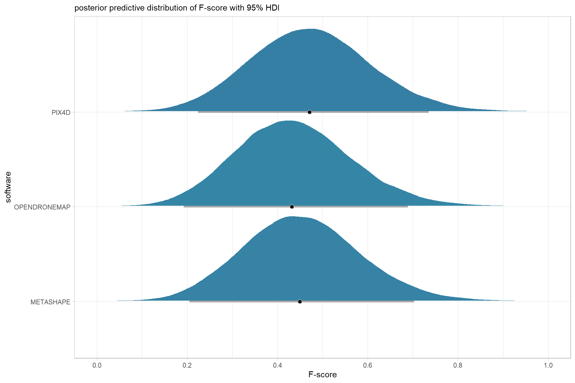
let’s compare these results to the results from our three nominal predictor model above and three nominal predictor + site effects model above
ptcld_validation_data %>%
  dplyr::distinct(software) %>%
  tidybayes::add_epred_draws(
    brms_f_mod5
    # this part is crucial
    , re_formula = ~ (1 | software)
  ) %>%
  dplyr::mutate(value = .epred, src = "brms_f_mod5") %>%
  dplyr::bind_rows(
    ptcld_validation_data %>%
      dplyr::distinct(software) %>%
      tidybayes::add_epred_draws(
        brms_f_mod4
        # this part is crucial
        , re_formula = ~ (1 | software)
      ) %>%
      dplyr::mutate(value = .epred, src = "brms_f_mod4")
    , ptcld_validation_data %>%
      dplyr::distinct(software) %>%
      tidybayes::add_epred_draws(
        brms_f_mod3
        # this part is crucial
        , re_formula = ~ (1 | software)
      ) %>%
      dplyr::mutate(value = .epred, src = "brms_f_mod3")
  ) %>%
  ggplot(mapping = aes(y = src, x = value, color = src, group = src)) +
  tidybayes::stat_pointinterval(position = "dodge") +
  facet_grid(rows = vars(software), switch = "y") +
  scale_y_discrete(NULL, breaks = NULL) +
  scale_color_manual(values = viridis::turbo(n = 6, begin = 0.2, end = 0.8)[3:5]) +
  labs(
    y = "", x = "F-score"
    , color = "model"
  ) +
  theme_light() +
  theme(legend.position = "top", strip.text = element_text(color = "black", face = "bold"))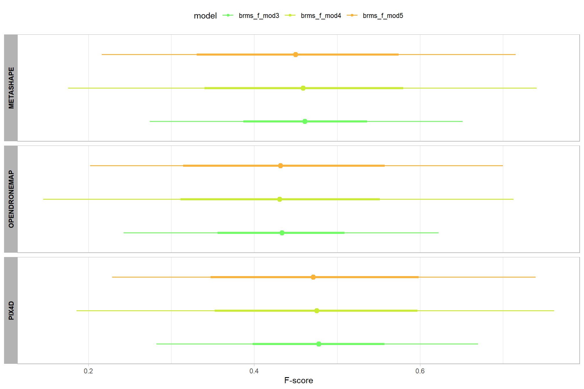
we can also perform pairwise comparisons after collapsing across the filtering mode, dense cloud quality setting, and study site to compare the software main effect
brms_contrast_temp =
  ptcld_validation_data %>%
    dplyr::distinct(software) %>%
    tidybayes::add_epred_draws(
      brms_f_mod5, allow_new_levels = T
      # this part is crucial
      , re_formula = ~ (1 | software)
    ) %>%
    dplyr::rename(value = .epred) %>%
    tidybayes::compare_levels(
      value
      , by = software
      , comparison = "pairwise"
    ) %>%
    dplyr::rename(contrast = software) %>%
  # median_hdi summary for coloring
  dplyr::group_by(contrast) %>%
  make_contrast_vars()

# what?
brms_contrast_temp %>% dplyr::glimpse()
## Rows: 120,000
## Columns: 16
## Groups: contrast [3]
## $ .chain <int> NA, NA, NA, NA, NA, NA, NA, NA, NA, NA, NA, NA, NA, N…
## $ .iteration <int> NA, NA, NA, NA, NA, NA, NA, NA, NA, NA, NA, NA, NA, N…
## $ .draw <int> 1, 2, 3, 4, 5, 6, 7, 8, 9, 10, 11, 12, 13, 14, 15, 16…
## $ contrast <chr> "OPENDRONEMAP - METASHAPE", "OPENDRONEMAP - METASHAPE…
## $ value <dbl> 0.014937640, 0.010701705, 0.032983125, 0.034905587, -…
## $ median_hdi_est <dbl> -0.008949634, -0.008949634, -0.008949634, -0.00894963…
## $ median_hdi_lower <dbl> -0.1611271, -0.1611271, -0.1611271, -0.1611271, -0.16…
## $ median_hdi_upper <dbl> 0.1125752, 0.1125752, 0.1125752, 0.1125752, 0.1125752…
## $ pr_gt_zero <chr> "40%", "40%", "40%", "40%", "40%", "40%", "40%", "40%…
## $ pr_lt_zero <chr> "60%", "60%", "60%", "60%", "60%", "60%", "60%", "60%…
## $ is_diff_dir <lgl> FALSE, FALSE, FALSE, FALSE, TRUE, FALSE, TRUE, TRUE, …
## $ pr_diff <dbl> 0.602925, 0.602925, 0.602925, 0.602925, 0.602925, 0.6…
## $ pr_diff_lab <chr> "Pr(MtaShp>ODM)=60%", "Pr(MtaShp>ODM)=60%", "Pr(MtaSh…
## $ pr_diff_lab_sm <chr> "Pr(<0)=60%", "Pr(<0)=60%", "Pr(<0)=60%", "Pr(<0)=60%…
## $ pr_diff_lab_pos <dbl> -0.1732117, -0.1732117, -0.1732117, -0.1732117, -0.17…
## $ sig_level <ord> <80%, <80%, <80%, <80%, <80%, <80%, <80%, <80%, <80%,…plot it
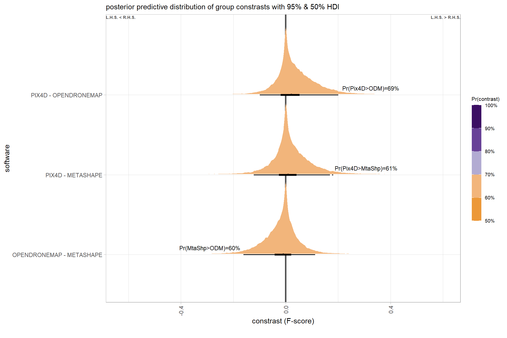
and summarize these contrasts
brms_contrast_temp %>%
  dplyr::group_by(contrast, pr_gt_zero) %>%
  tidybayes::median_hdi(value) %>%
  dplyr::arrange(contrast) %>%
  dplyr::select(contrast, value, .lower, .upper, pr_gt_zero) %>%

  kableExtra::kbl(
    digits = 2
    , caption = "brms::brm model: 95% HDI of the posterior predictive distribution of group constrasts"
    , col.names = c(
      "software contrast"
      , "difference (F-score)"
      , "HDI low", "HDI high"
      , "Pr(diff>0)"
    )
  ) %>%
kableExtra::kable_styling()| software contrast | difference (F-score) | HDI low | HDI high | Pr(diff>0) |
|---|---|---|---|---|
| OPENDRONEMAP - METASHAPE | -0.01 | -0.16 | 0.11 | 40% |
| PIX4D - METASHAPE | 0.01 | -0.12 | 0.17 | 61% |
| PIX4D - METASHAPE | 0.01 | 0.18 | 0.18 | 61% |
| PIX4D - OPENDRONEMAP | 0.02 | -0.10 | 0.20 | 69% |
6.7.2.11 \(\sigma\) posteriors
Finally, we can quantify the variation in F-score by comparing the \(\sigma\) (sd) posteriors
unsure about the scale of the \(\sigma\) parameters are on in the beta model. Here, we invert the logit sd values from the model using plogis() which converts the parameter values to a probability/proportion (e.g.; 0-1) because they are parameters of the intercept and interaction effects so must be on the transformed (link = "logit") scale…double check
For a phenomenally excellent overview of binary logistic regression and how to interpret coefficients, see Steven Miller’s most excellent lab script here
# tidybayes::get_variables(brms_f_mod5)
# extract the posterior draws
# extract the posterior draws
  brms::as_draws_df(brms_f_mod5) %>%
    dplyr::select(c(tidyselect::starts_with("sd_"))) %>%
    tidyr::pivot_longer(dplyr::everything()) %>%
    # dplyr::group_by(name) %>%
    # tidybayes::median_hdi(value) %>%
    dplyr::mutate(
      name = name %>%
        stringr::str_replace_all("depth_maps_generation_quality", "quality") %>%
        stringr::str_replace_all("depth_maps_generation_filtering_mode", "filtering") %>%
        stringr::str_remove_all("sd_") %>%
        stringr::str_remove_all("__Intercept") %>%
        stringr::str_replace_all("_", " ") %>%
        forcats::fct_reorder(value)
    ) %>%
  # plot
    ggplot(aes(x = value, y = name)) +
    tidybayes::stat_dotsinterval(
      point_interval = median_hdi, .width = .95
      , justification = -0.04
      , shape = 21 #, point_size = 3
      , quantiles = 100
    ) +
    scale_x_continuous(breaks = NULL) +
    labs(x = "", y = ""
      , subtitle = latex2exp::TeX("$\\sigma_\\beta$ posterior distributions")
      , title = "F-Score"
    ) +
    theme_light() +
    theme(
      plot.subtitle = element_text(size = 8)
      , plot.title = element_text(size = 9)
    )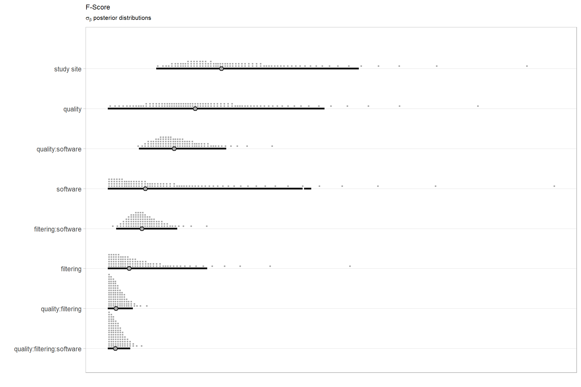
Variance of study site is stronger than variance of depth map generation quality, but the posterior predictive distributions overlap a good deal. The study site (the “subjects” in our study) seems to have the overall strongest effect, but this comes with high uncertainty. Taken alone, the influence of quality, filtering, and software comes with huge uncertainty. This makes sense as the influence of software largely depends on the depth map generation quality, of which we are fairly certain. Filtering mode has the overall weakest effect on tree detection and this comes with relatively high certainty, especially conditional on the depth map generation quality.
and perform model selection via information criteria with the brms::loo_compare() function
brms_f_mod5 = brms::add_criterion(brms_f_mod5, criterion = c("loo", "waic"))
brms::loo_compare(brms_f_mod1, brms_f_mod2, brms_f_mod3, brms_f_mod4, brms_f_mod5, criterion = "loo")
## elpd_diff se_diff
## brms_f_mod5 0.0 0.0
## brms_f_mod4 -1.1 6.3
## brms_f_mod3 -92.0 11.5
## brms_f_mod1 -92.4 11.2
## brms_f_mod2 -94.1 11.26.7.2.12 Additional Plots for Export
patchwork of F-score contrasts
layout_temp = c(
    # area(t, l, b, r)
    patchwork::area(2, 1, 2, 1)
    , patchwork::area(2, 3, 2, 3)
    , patchwork::area(4, 1, 4, 3)
  )
  # check the layout
  # plot(layout_temp)
############################
# patchwork for height
############################
  ptchwrk_qlty_sftwr_comp +
    labs(subtitle = "A: Quality Contrast by Software") +
    theme(plot.background = element_rect(colour = "gray88", fill=NA, size=3)) +
  ptchwrk_fltr_sftwr_comp +
    labs(subtitle = "B: Filtering Mode Contrast by Software") +
    theme(plot.background = element_rect(colour = "gray88", fill=NA, size=3)) +
  patchwork::free(
    ptchwrk_sftwr_qlty_comp +
    labs(subtitle = "C: Software Contrast by Quality") +
    theme(plot.background = element_rect(colour = "gray88", fill=NA, size=3)) ) +
  # plot_annotation(tag_levels = list(c('#', '&'), '1')) +
  patchwork::plot_layout(
    design = layout_temp
    , widths = c(1,0.01,1)
    , heights = c(0.01,1,0.01,1,0.01)
  ) &
  scale_x_continuous(
    limits = c(-0.58,0.96)
    , breaks = seq(-0.8,0.8,0.4)
    , labels = seq(-0.8,0.8,0.4) %>% scales::number(accuracy = 0.1)
  ) &
  theme(
    axis.title.y = element_blank()
    , plot.subtitle = element_text(face = "bold", hjust = 0.0)
    # , plot.background = element_rect(colour = "gray88", fill=NA, size=3)
  )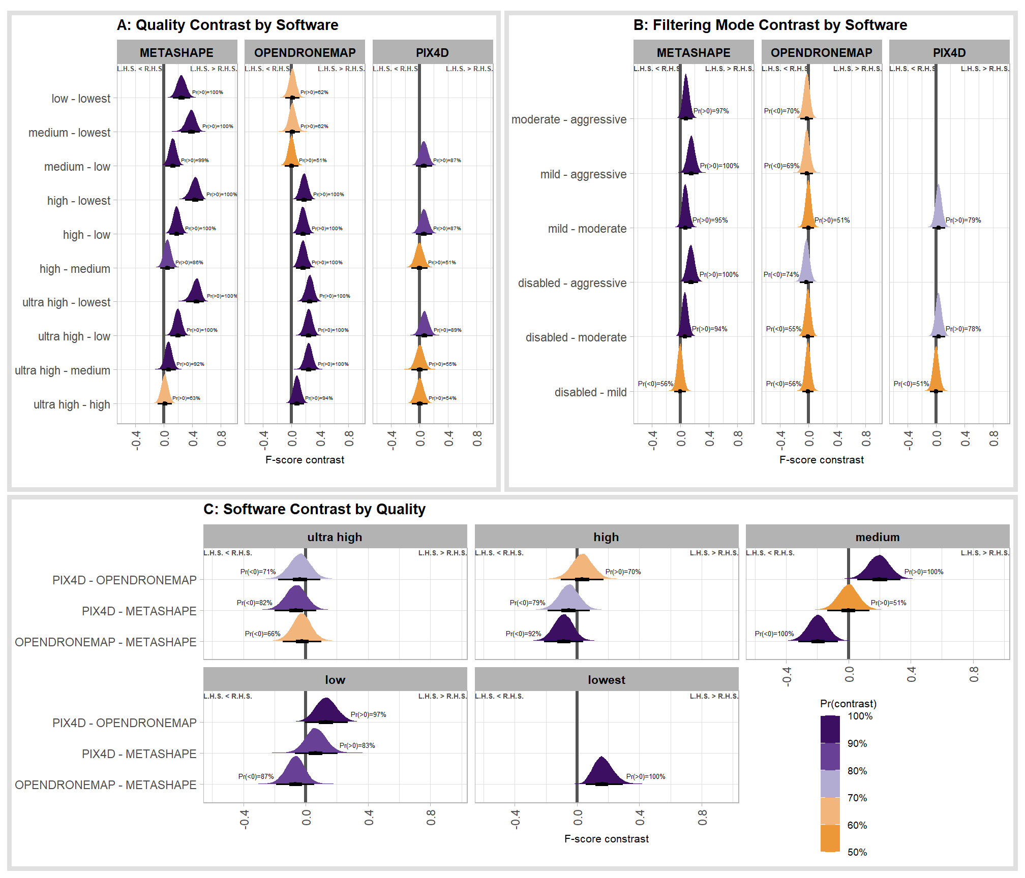
6.8 Heterogeneous variances and robustness against outliers
In our previous model of the data \(y_i\) described by a beta distribution with three nominal predictors and site effects our posterior predictive checks indicated potential improvements for our model fit.
Kruschke (2015) notes:
As was mentioned earlier in the chapter, we have assumed normally distributed data within groups, and equal variances across the groups, merely for simplicity and for consistency with traditional ANOVA. We can relax those assumptions in Bayesian software. In this section, we use t distributed noise instead of normal distributions, and we provide every group with its own standard-deviation parameter. Moreover, we put a hierarchical prior on the standard-deviation parameters, so that each group mutually informs the standard deviations of the other groups via the higher-level distribution…Instead of there being a single \(\sigma_y\) parameter that applies to all groups, each group has its own scale parameter, \(\sigma_j\). (p. 573-574)
and see section 20 from Kurz’s ebook supplement
6.8.1 Bayesian
With the beta likelihood our model with three nominal predictor variables, subject-level effects, and heterogeneous variances and robustness against outliers the model becomes:
\[\begin{align*} y_{i} \sim & \operatorname{Beta} \bigl(\mu_{i}, , \phi_{[jkf](i)} \bigr) \\ \operatorname{logit}(\mu_{i}) = & \beta_0 \\ & + \sum_{j} \beta_{1[j]} x_{1[j]} + \sum_{k} \beta_{2[k]} x_{2[k]} + \sum_{f} \beta_{3[f]} x_{3[f]} + \sum_{s} \beta_{4[s]} x_{4[s]} \\ & + \sum_{j,k} \beta_{1\times2[j,k]} x_{1\times2[j,k]} + \sum_{j,f} \beta_{1\times3[j,f]} x_{1\times3[j,f]} + \sum_{k,f} \beta_{2\times3[k,f]} x_{2\times3[k,f]} \\ & + \sum_{j,k,f} \beta_{1\times2\times3[j,k,f]} x_{1\times2\times3[j,k,f]} \\ \beta_{0} \sim & \operatorname{Normal}(0,1) \\ \beta_{1[j]} \sim & \operatorname{Normal}(0,\sigma_{\beta_{1}}) \\ \beta_{2[k]} \sim & \operatorname{Normal}(0,\sigma_{\beta_{2}}) \\ \beta_{3[f]} \sim & \operatorname{Normal}(0,\sigma_{\beta_{3}}) \\ \beta_{4[s]} \sim & \operatorname{Normal}(0,\sigma_{\beta_{4}}) \\ \beta_{1\times2[j,k]} \sim & \operatorname{Normal}(0,\sigma_{\beta_{1\times2}}) \\ \beta_{1\times3[j,f]} \sim & \operatorname{Normal}(0,\sigma_{\beta_{1\times3}}) \\ \beta_{2\times3[k,f]} \sim & \operatorname{Normal}(0,\sigma_{\beta_{2\times3}}) \\ \sigma_{\beta_{1}} \sim & \operatorname{Gamma}(1.28,0.005) \\ \sigma_{\beta_{2}} \sim & \operatorname{Gamma}(1.28,0.005) \\ \sigma_{\beta_{3}} \sim & \operatorname{Gamma}(1.28,0.005) \\ \sigma_{\beta_{4}} \sim & \operatorname{Gamma}(1.28,0.005) \\ \sigma_{\beta_{1\times2}} \sim & \operatorname{Gamma}(1.28,0.005) \\ \sigma_{\beta_{1\times3}} \sim & \operatorname{Gamma}(1.28,0.005) \\ \sigma_{\beta_{2\times3}} \sim & \operatorname{Gamma}(1.28,0.005) \\ \phi_{[jkf](i)} \sim & \operatorname{Gamma}(\alpha,\theta) \\ \alpha \sim & {\sf XXX} (xxx,xxx) \\ \theta \sim & {\sf XXX} (xxx,xxx) \end{align*}\]
!!!! Need to check how our \(\phi_{[jkf](i)}\) is distributed
, where \(j\) is the depth map generation quality setting corresponding to observation \(i\), \(k\) is the depth map filtering mode setting corresponding to observation \(i\), \(f\) is the processing software corresponding to observation \(i\), and \(s\) is the study site corresponding to observation \(i\)
brms allows us to model the precision (\(\phi\)) but it is not required. If \(\phi\) is not modeled, you still get a precision component, but it is universal across all the different coefficients (it doesn’t vary across any variables in the model). Heiss explains that:
for whatever mathy reasons, when you don’t explicitly model the precision, the resulting coefficient in the table isn’t on the log scale—it’s a regular non-logged number, so there’s no need to exponentiate.
in thie brms community post it is similarly noted that:
If you don’t predict the parameters, you give priors for them on non-transformed scale. When you predict them, the predictors become linear coefficients as any other and work on the transformed scale - the transformations are specified by the link_XX parameters of the families (and you can change them if you need).
Need to check our prior selection…just go with brms defaults for now
Now fit the model.
brms_f_mod5_5 = brms::brm(
  formula = brms::bf(
  ### model for y
    f_score ~
    # baseline
    1 +
    # main effects
    (1 | depth_maps_generation_quality) +
    (1 | depth_maps_generation_filtering_mode) +
    (1 | software) +
    (1 | study_site) + # only fitting main effects of site and not interactions
    # two-way interactions
    (1 | depth_maps_generation_quality:depth_maps_generation_filtering_mode) +
    (1 | depth_maps_generation_quality:software) +
    (1 | depth_maps_generation_filtering_mode:software) +
    # three-way interactions
    (1 | depth_maps_generation_quality:depth_maps_generation_filtering_mode:software)
  ### model for phi
    , phi  ~ 1 + (1 | depth_maps_generation_quality:depth_maps_generation_filtering_mode:software)
  )
  , data = ptcld_validation_data
  , family = Beta(link = "logit")
  , iter = 20000, warmup = 10000, chains = 4
  , control = list(adapt_delta = 0.999, max_treedepth = 13)
  , cores = round(parallel::detectCores()/2)
  , file = paste0(rootdir, "/fits/brms_f_mod5_5")
)
# brms::make_stancode(brms_f_mod5_5)
# print(brms_f_mod5_5)
# brms::prior_summary(brms_f_mod5_5)
6.8.1.1 Posterior Predictive Checks
Markov chain Monte Carlo (MCMC) simulations were conducted using the brms package (Bürkner 2017) to estimate posterior predictive distributions of the parameters of interest. We ran three chains of 100,000 iterations with the first 50,000 discarded as burn-in. Trace-plots were utilized to visually assess model convergence and sufficient convergence was checked with \(\hat{R}\) values near 1 (Brooks & Gelman, 1998). Posterior predictive checks were used to evaluate model goodness-of-fit by comparing data simulated from the model with the observed data used to estimate the model parameters (Hobbs & Hooten, 2015). Calculating the proportion of MCMC iterations in which the test statistic (i.e., mean and sum of squares) from the simulated data and observed data are more extreme than one another provides the Bayesian P-value. Lack of fit is indicated by a value close to 0 or 1 while a value of 0.5 indicates perfect fit (Hobbs & Hooten, 2015).
To learn more about this approach to posterior predictive checks, check out Gabry’s (2022) vignette, Graphical posterior predictive checks using the bayesplot package.
check the trace plots for problems with convergence of the Markov chains
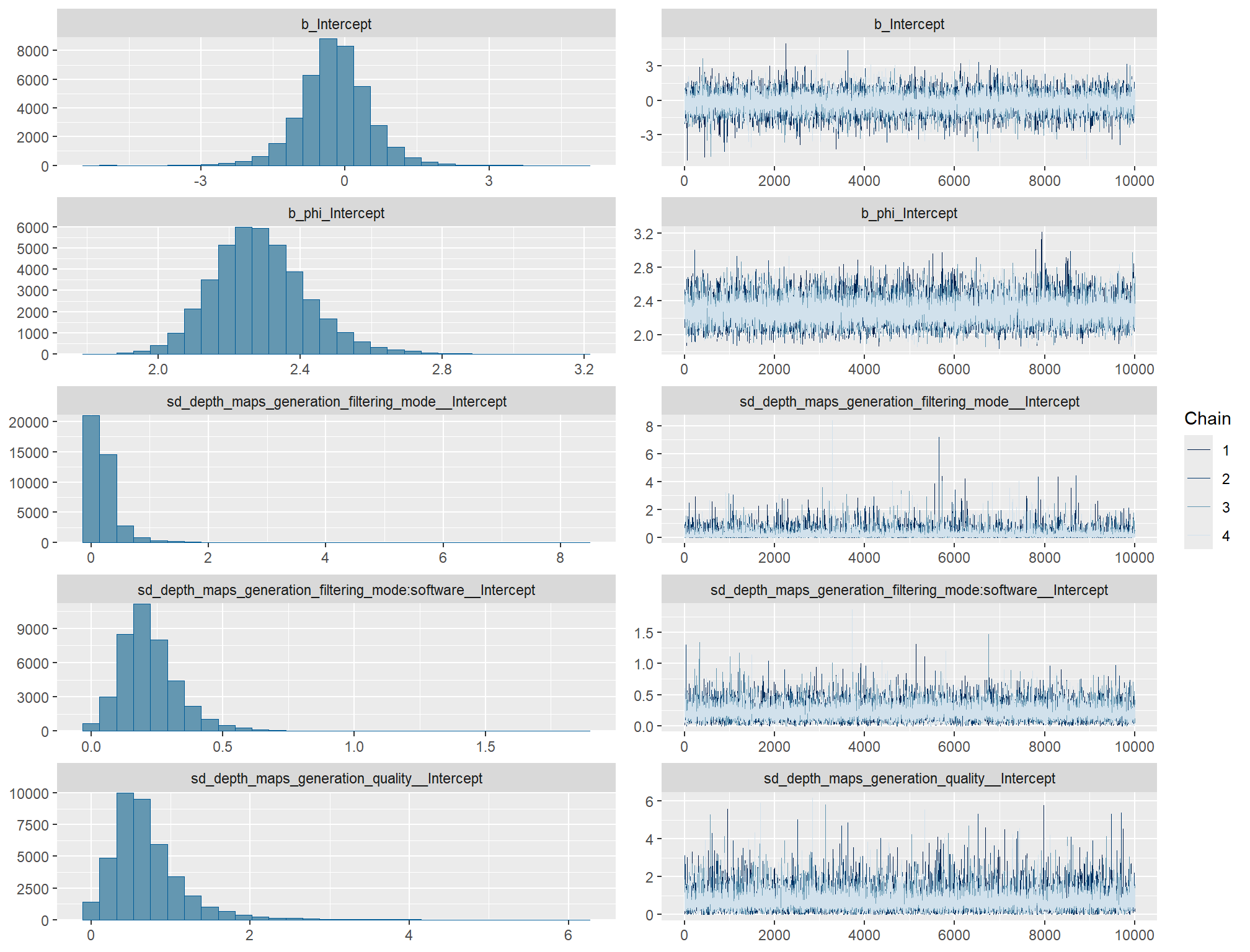
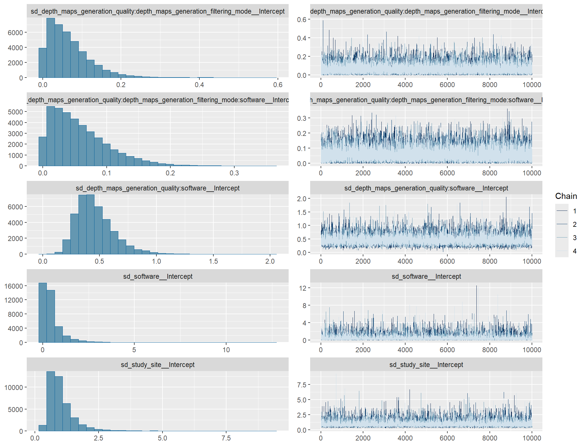
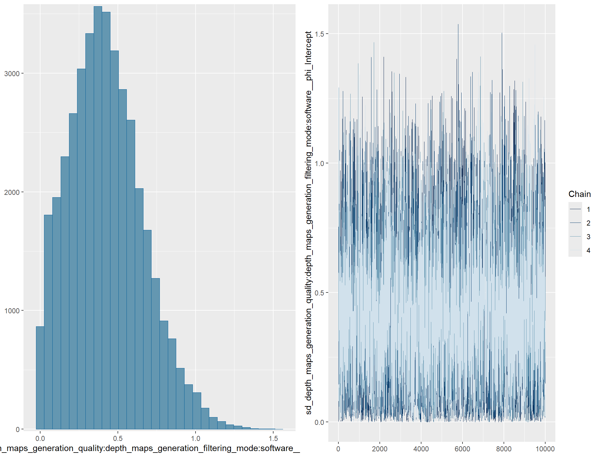
and check our \(\hat{R}\) values
brms_f_mod5_5 %>%
  brms::rhat() %>%
  as.data.frame() %>%
  tibble::rownames_to_column(var = "parameter") %>%
  dplyr::rename_with(tolower) %>%
  dplyr::rename(rhat = 2) %>%
  dplyr::filter(
    stringr::str_starts(parameter, "b_")
    | stringr::str_starts(parameter, "r_")
    | stringr::str_starts(parameter, "sd_")
    | parameter == "phi"
  ) %>%
  dplyr::mutate(
    parameter = parameter %>%
      stringr::str_replace_all("depth_maps_generation_quality", "quality") %>%
      stringr::str_replace_all("depth_maps_generation_filtering_mode", "filtering")
    , chk = (rhat <= 1*0.998 | rhat >= 1*1.002)
  ) %>%
  ggplot(aes(x = rhat, y = parameter, color = chk, fill = chk)) +
  geom_vline(xintercept = 1, linetype = "dashed", color = "gray44", lwd = 1.2) +
  geom_vline(xintercept = 1*0.998, lwd = 1.5) +
  geom_vline(xintercept = 1*1.002, lwd = 1.5) +
  geom_vline(xintercept = 1*0.999, lwd = 1.2, color = "gray33") +
  geom_vline(xintercept = 1*1.001, lwd = 1.2, color = "gray33") +
  geom_point() +
  scale_fill_manual(values = c("navy", "firebrick")) +
  scale_color_manual(values = c("navy", "firebrick")) +
  labs(
    x = latex2exp::TeX("$\\hat{R}$")
    , subtitle = latex2exp::TeX("posterior-predictive check for parameter $\\hat{R}$ estimates")
  ) +
  theme_light() +
  theme(
    legend.position = "none"
    , axis.text.y = element_text(size = 4)
    , panel.grid.major.x = element_blank()
    , panel.grid.minor.x = element_blank()
  )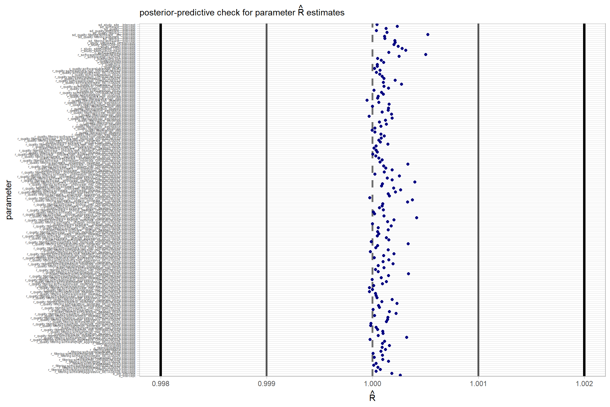
posterior-predictive check to make sure the model does an okay job simulating data that resemble the sample data
# posterior predictive check
brms::pp_check(
    brms_f_mod5_5
    , type = "dens_overlay"
    , ndraws = 100
  ) +
  labs(subtitle = "posterior-predictive check (overlaid densities)") +
  theme_light() +
  scale_y_continuous(NULL, breaks = NULL) +
  theme(
    legend.position = "top", legend.direction = "horizontal"
    , legend.text = element_text(size = 14)
  )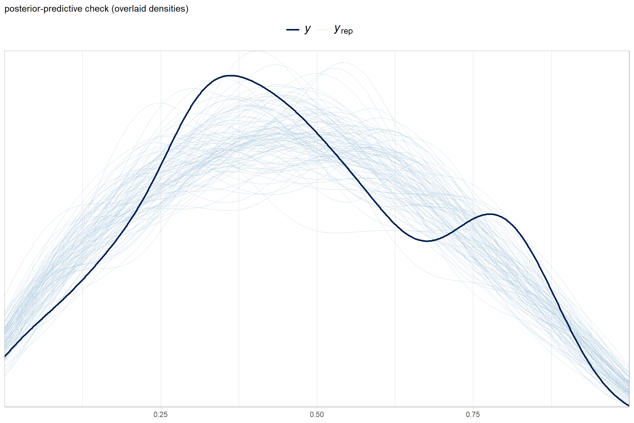
another way
brms::pp_check(brms_f_mod5_5, type = "ecdf_overlay", ndraws = 100) +
  labs(subtitle = "posterior-predictive check (ECDF: empirical cumulative distribution function)") +
  theme_light() +
  theme(
    legend.position = "top", legend.direction = "horizontal"
    , legend.text = element_text(size = 14)
  )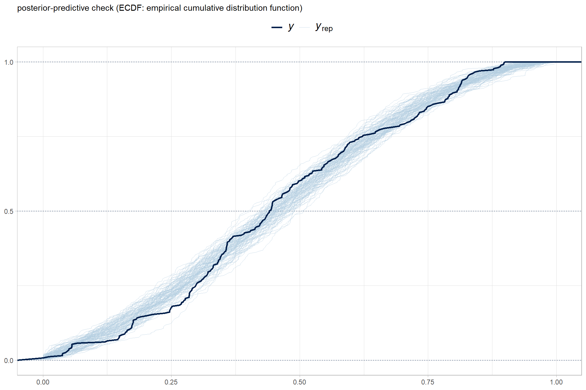
and another posterior predictive check for the overall model
# means
p1_temp = brms::pp_check(
    brms_f_mod5_5
    , type = "stat"
    , stat = "mean"
  ) +
  scale_y_continuous(NULL, breaks = c(NULL)) +
  labs(subtitle = "means") +
  theme_light()
# sds
p2_temp = brms::pp_check(
    brms_f_mod5_5
    , type = "stat"
    , stat = "sd"
  ) +
  scale_y_continuous(NULL, breaks = c(NULL)) +
  labs(subtitle = "sd's") +
  theme_light()

# combine
(p1_temp + p2_temp) &
  theme(legend.position = "none") &
  plot_annotation(
    title = "Posterior-predictive statistical checks\noverall model"
    , subtitle = expression(
      "The dark blue lines are "*italic(T(y))*", and the light blue bars are for "*italic(T)(italic(y)[rep])*".")
  )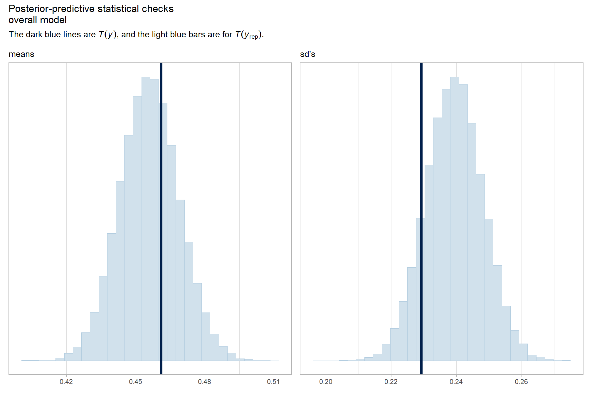
and another posterior predictive check for the overall model combining mean and sd
brms::pp_check(brms_f_mod5_5, type = "stat_2d") +
  theme_light() +
  theme(
    legend.position = "top", legend.direction = "horizontal"
    , legend.text = element_text(size = 14)
  )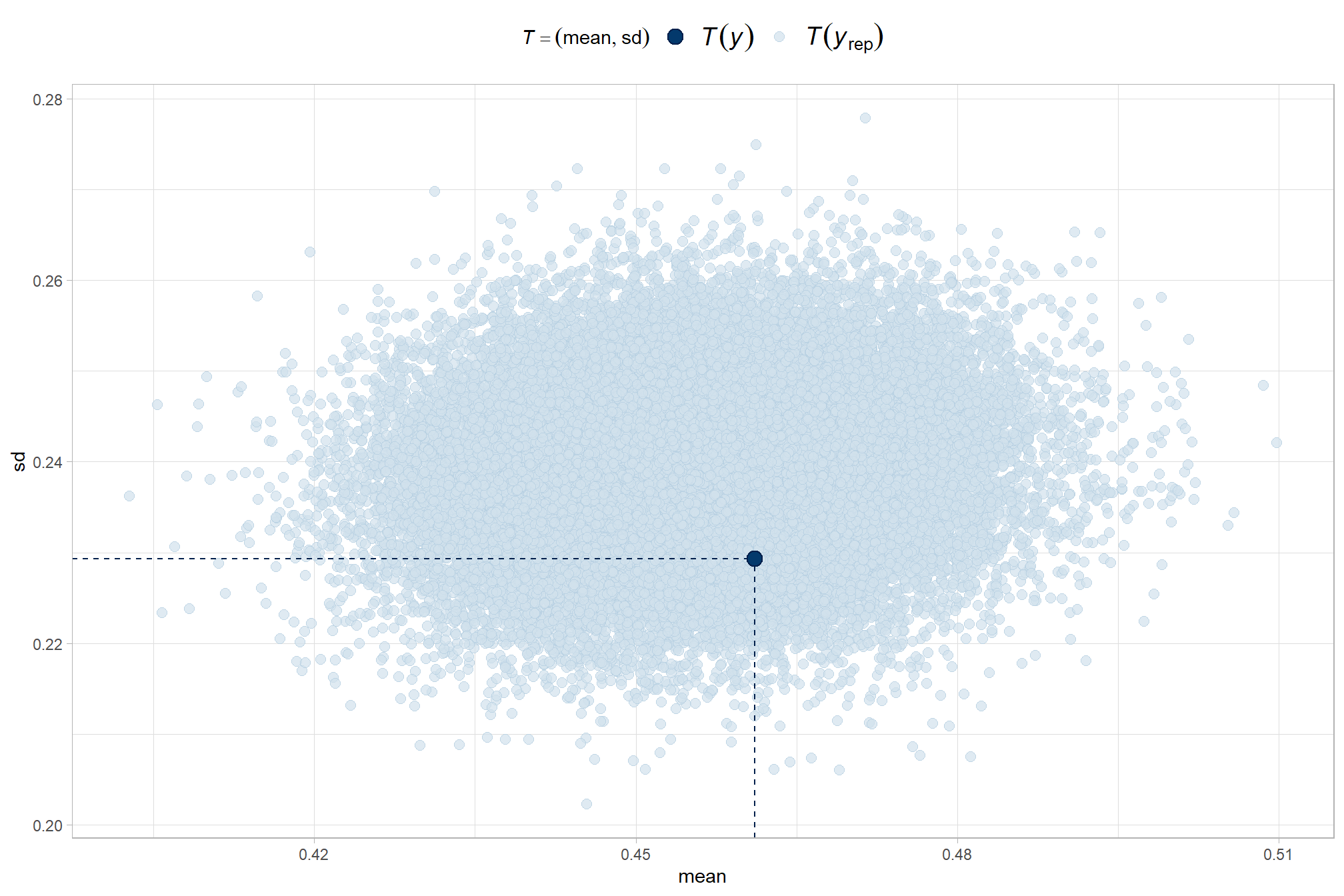
How’d we do capturing the conditional means and standard deviations by depth map generation quality?
# means
p1_temp = brms::pp_check(
    brms_f_mod5_5
    , type = "stat_grouped" # "dens_overlay_grouped"
    , stat = "mean"
    , group = "depth_maps_generation_quality"
  ) +
  scale_y_continuous(NULL, breaks = c(NULL)) +
  labs(subtitle = "means") +
  facet_grid(cols = vars(group), scales = "free") +
  theme_light()
# sds
p2_temp = brms::pp_check(
    brms_f_mod5_5
    , type = "stat_grouped" # "dens_overlay_grouped"
    , stat = "sd"
    , group = "depth_maps_generation_quality"
  ) +
  scale_y_continuous(NULL, breaks = c(NULL)) +
  labs(subtitle = "sd's") +
  facet_grid(cols = vars(group), scales = "free") +
  theme_light()
# combine
(p1_temp / p2_temp) &
  theme(legend.position = "none") &
  plot_annotation(
    title = "Posterior-predictive statistical checks\nby dense cloud quality"
    , subtitle = expression(
      "The dark blue lines are "*italic(T(y))*", and the light blue bars are for "*italic(T)(italic(y)[rep])*".")
  )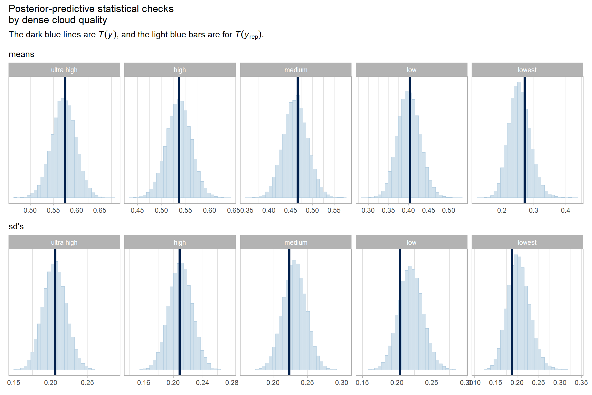
Both the means and sd’s of the F-score are well represented across the different levels of dense cloud quality
What about for the software?
pp_check(brms_f_mod5_5, "dens_overlay_grouped", group = "software", ndraws = 100) +
  labs(subtitle = "posterior-predictive check (overlaid densities)\nby software") +
  theme_light() +
  scale_y_continuous(NULL, breaks = NULL) +
  theme(
    legend.position = "top", legend.direction = "horizontal"
    , legend.text = element_text(size = 14)
  )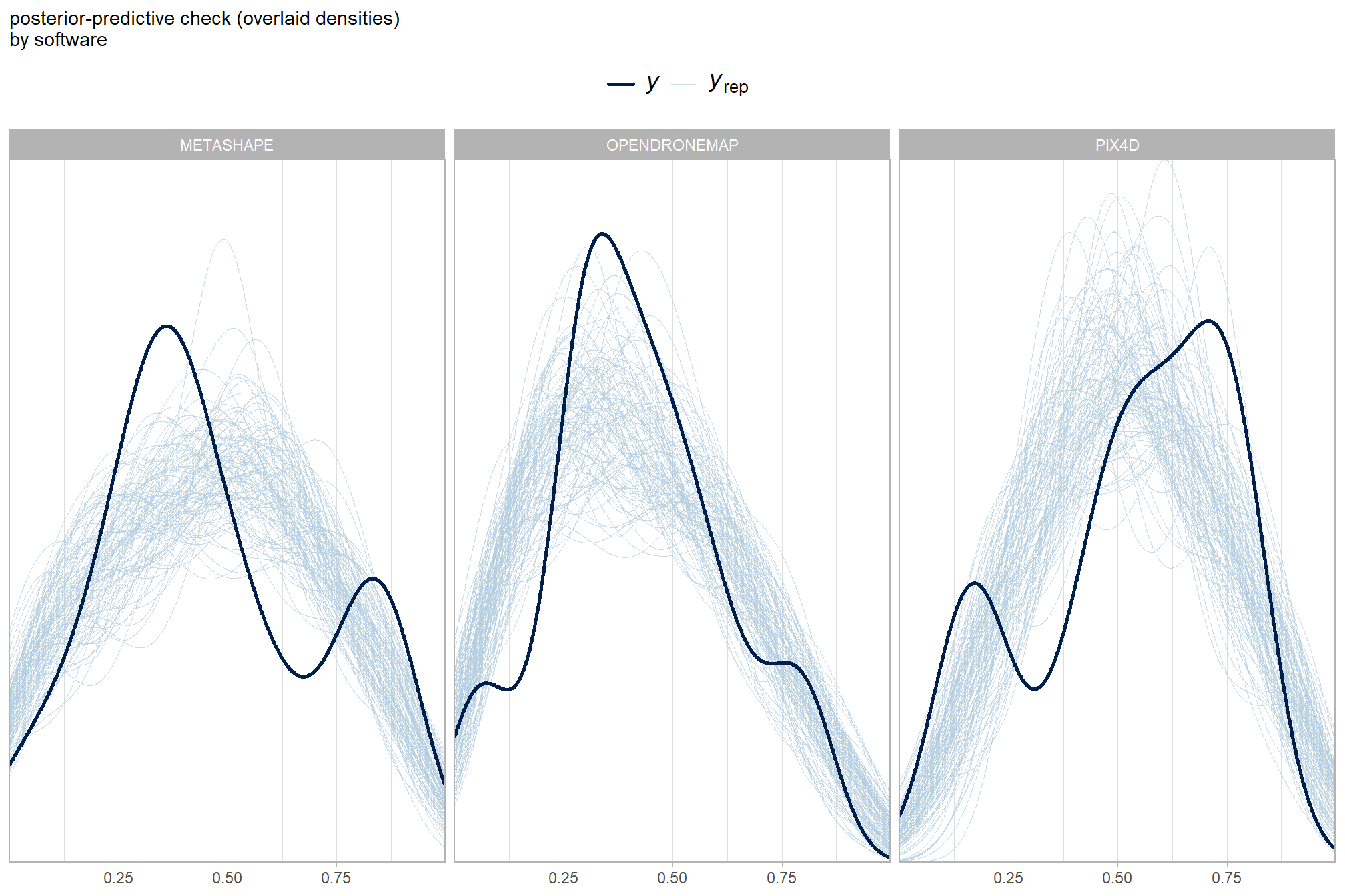
and what about for the filtering mode?
pp_check(brms_f_mod5_5, "dens_overlay_grouped", group = "depth_maps_generation_filtering_mode", ndraws = 100) +
  labs(subtitle = "posterior-predictive check (overlaid densities)\nby filtering mode") +
  theme_light() +
  scale_y_continuous(NULL, breaks = NULL) +
  theme(
    legend.position = "top", legend.direction = "horizontal"
    , legend.text = element_text(size = 14)
  )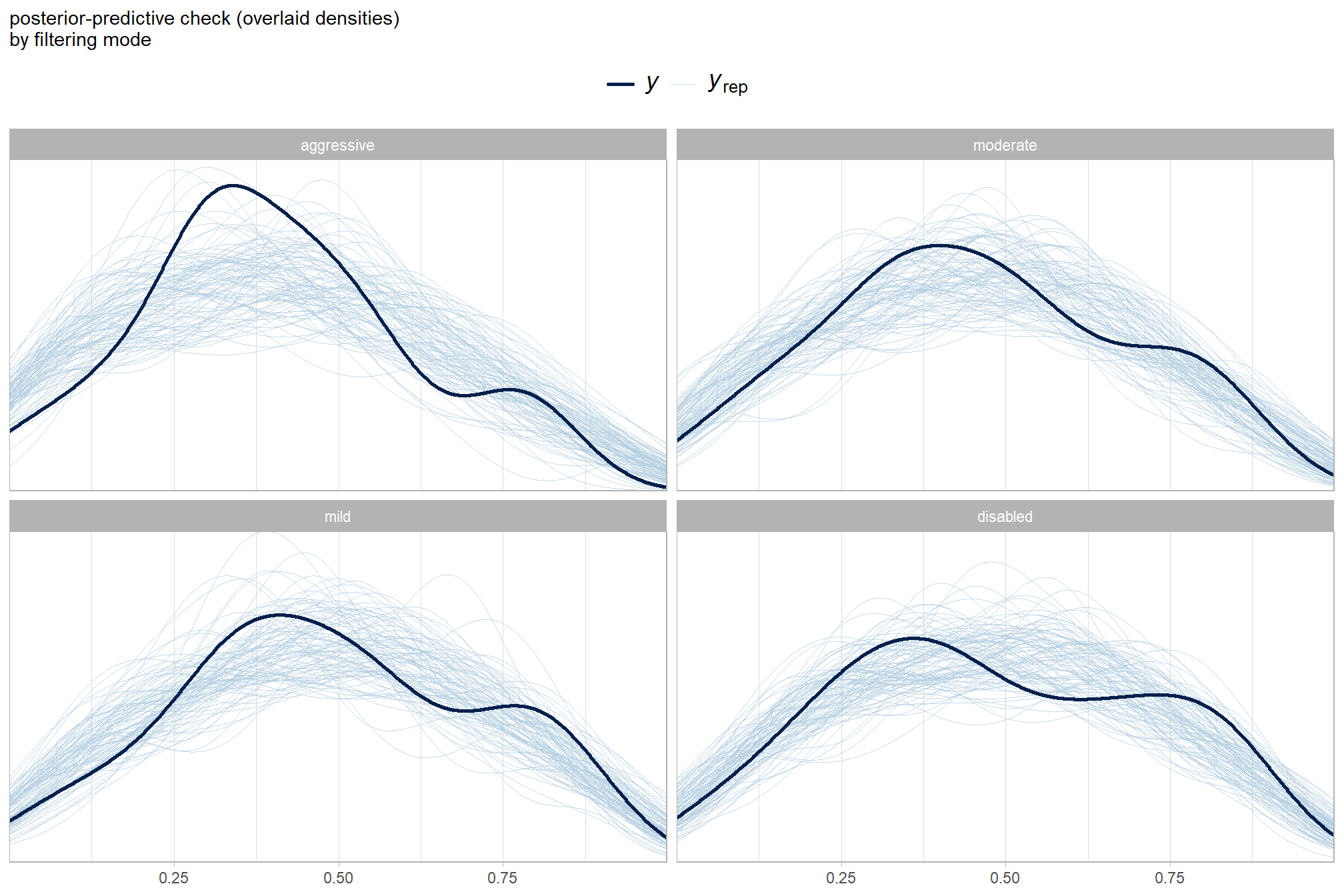
We didn’t see much change in our posterior predictive checks compared to our previous model of the data \(y_i\) described by a beta distribution with three nominal predictors and site effects our posterior predictive checks.
The Bayesian p-value is the probability that a test statistic in the reference distribution exceeds its value in the data. The Bayesian p-value is calculated from the posterior predictive distribution of the new data and the distribution of the observed data. We estimate the probability that the test statistic calculated from “new” data arising from our model (\(y_{new}\)) is more extreme than the test statistic calculated from the observed data (\(y\)): \(\text{P-value}(y) = Pr(T(y_{new}) > T(y))\) where the test statistic \(T(y)\) describes the distribution of the data as a summary of the data; it could be the mean, variance, the coefficient of variation, the kurtosis, the maximum, or the minimum of the observed data set, or it might be an “omnibus” statistic like a squared discrepancy or a chi-square value Hobbs and Hooten (2015, p. 188)
Bayesian P values for mean and standard deviation test statistics The P values for the mean (P mean) give the probability that the mean of the data of new, out-of-sample observations simulated from the model exceeds the mean of the observed data. The P values for the standard deviation (P SD) give the probability that the standard deviation of new, out-of-sample observations simulated from the model exceeds the standard deviation of the observed data. Large (\(\gtrapprox 0.90\)) or small (\(\lessapprox 0.10\)) values indicate lack of fit. Hobbs and Hooten (2015);Hobbs et al. (2024, Appendix S2 p. 8)
Check the Bayesian p-values between the models
# bayesian p-value
get_mod_p_val = function(my_mod, ndraws = 1000){
  # get draws from the posterior predictive distribution
  brms::posterior_predict(my_mod, ndraws = ndraws) %>%
    dplyr::as_tibble() %>%
    dplyr::mutate(draw = dplyr::row_number()) %>%
    tidyr::pivot_longer(cols = -draw, values_to = "y_rep") %>%
    dplyr::mutate(y_n = readr::parse_number(name)) %>%
    dplyr::select(-c(y_n)) %>%
    dplyr::group_by(draw) %>%
    # make test statistic
    dplyr::summarise(
      # test statistics y_sim
      mean_y_rep = mean(y_rep)
      , sd_y_rep = sd(y_rep)
    ) %>%
    # # observed data test statistics
    dplyr::mutate(
    # test statistics y
      mean_y = mean(my_mod$data[,1])
      , sd_y = sd(my_mod$data[,1])
    ) %>%
    # p-values
    dplyr::ungroup() %>%
    dplyr::mutate(
      p_val_mean = as.numeric(mean_y_rep > mean_y)
      , p_val_sd = as.numeric(sd_y_rep > sd_y)
    ) %>%
    # summarize p-vals
    dplyr::summarise(
      P.mean = mean(p_val_mean)
      , P.sd = mean(p_val_sd)
    )
}
# get the model p-values
set.seed(16) # replicate results
dplyr::bind_rows(
    get_mod_p_val(brms_f_mod4, ndraws = 5000) %>%
      dplyr::mutate(model = "brms_f_mod4")
    , get_mod_p_val(brms_f_mod5, ndraws = 5000) %>%
      dplyr::mutate(model = "brms_f_mod5")
    , get_mod_p_val(brms_f_mod5_5, ndraws = 5000) %>%
      dplyr::mutate(model = "brms_f_mod5_5")
  ) %>%
  dplyr::relocate(model) %>%
  kableExtra::kbl(digits = 3) %>%
kableExtra::kable_styling()| model | P.mean | P.sd |
|---|---|---|
| brms_f_mod4 | 0.488 | 0.612 |
| brms_f_mod5 | 0.224 | 0.881 |
| brms_f_mod5_5 | 0.342 | 0.876 |
perhaps we should use brms_f_mod4 in which we modeled F-score presuming a Gaussian likelihood??? What are the pros and cons? Surely, an accurate representation of the \(y_i\) data (as represented by the beta distribution) is meaningful even if “worse” p-values are found.
let’s perform model selection via information criteria with the brms::loo_compare() function to check
brms_f_mod5_5 = brms::add_criterion(brms_f_mod5_5, criterion = c("loo", "waic"))
brms::loo_compare(brms_f_mod1, brms_f_mod2, brms_f_mod3, brms_f_mod4, brms_f_mod5, brms_f_mod5_5, criterion = "loo")
## elpd_diff se_diff
## brms_f_mod5 0.0 0.0
## brms_f_mod4 -1.1 6.3
## brms_f_mod5_5 -7.4 4.3
## brms_f_mod3 -92.0 11.5
## brms_f_mod1 -92.4 11.2
## brms_f_mod2 -94.1 11.2The information criteria suggests that we continue with brms_f_mod5 in which \(y_i\) is described by a beta distribution with three nominal predictors and site effects and we did not model dispersion, instead using a single \(\phi_y\) parameter that applies to all groups
6.9 Overstory and Understory Validation
In our validation data creation process we calculated F-score for overstory and understory trees separately.
Here, let’s add a factor variable with levels for overstory and understory as a predictor to our final model from above.
The overall F-score is not the same as combining the overstory and understory F-score by calculating the mean of these values due to the differing number of observations in each. To build this model we need to convert our data to long format so that a row is also unique by our overstory/understory factor.
Each study site contributes one observation per dense cloud quality, filtering mode, software, and overstory/understory factor. That is, a row in the underlying data is unique by study site, software, dense cloud quality, filtering mode, and overstory/understory factor.
6.9.1 Summary Statistics
ou_ptcld_validation_data =
  ptcld_validation_data %>%
  dplyr::select(
    study_site, software
    , depth_maps_generation_quality
    , depth_maps_generation_filtering_mode
    # our dependent var in wide format
    , understory_f_score, overstory_f_score
  ) %>%
  tidyr::pivot_longer(
    cols = tidyselect::ends_with("_f_score")
    , names_to = "story"
    , values_to = "f_score"
    , values_drop_na = F
  ) %>%
  dplyr::mutate(
    story = story %>% stringr::str_remove_all("_f_score") %>% factor()
  )
# what is this data?
ou_ptcld_validation_data %>% dplyr::glimpse()
## Rows: 520
## Columns: 6
## $ study_site <chr> "KAIBAB_HIGH", "KAIBAB_HIGH", "KA…
## $ software <chr> "METASHAPE", "METASHAPE", "METASH…
## $ depth_maps_generation_quality <ord> high, high, high, high, high, hig…
## $ depth_maps_generation_filtering_mode <ord> aggressive, aggressive, disabled,…
## $ story <fct> understory, overstory, understory…
## $ f_score <dbl> 0.2634731, 0.3461179, 0.4105263, …# a row is unique by...
identical(
nrow(ou_ptcld_validation_data)
, ou_ptcld_validation_data %>%
dplyr::distinct(
study_site, software
, depth_maps_generation_quality
, depth_maps_generation_filtering_mode
, story
) %>%
nrow()
)## [1] TRUE# and we should have 2 times the rows as the orignial data
identical(
nrow(ou_ptcld_validation_data) %>% as.numeric() # long data
, nrow(ptcld_validation_data)*2 %>% as.numeric() # original wide data
)## [1] TRUEquick summary stats
##  overstory_f_score understory_f_score
##  Min.   :0.0001    Min.   :0.0001
##  1st Qu.:0.3250    1st Qu.:0.1372
##  Median :0.4992    Median :0.3448
##  Mean   :0.5163    Mean   :0.3271
##  3rd Qu.:0.7297    3rd Qu.:0.5046
##  Max.   :0.9408    Max.   :0.7419
let’s check this data with our geom_tile plot
# create function for combining plots with patchwork
plt_tile_fn_temp = function(ss = "overstory"){
  ou_ptcld_validation_data %>%
    dplyr::filter(tolower(story) == tolower(ss)) %>%
    dplyr::group_by(story, software, depth_maps_generation_quality, depth_maps_generation_filtering_mode) %>%
    # collapse across study site
    dplyr::summarise(
      mean_f_score = mean(f_score, na.rm = T)
      # , med_f_score = median(f_score, na.rm = T)
      , sd_f_score = sd(f_score, na.rm = T)
      , n = dplyr::n()
    ) %>%
    ggplot(mapping = aes(
      y = depth_maps_generation_quality
      , x = depth_maps_generation_filtering_mode
      , fill = mean_f_score
      , label = paste0(scales::comma(mean_f_score,accuracy = 0.01), "\n(n=", n,")")
    )) +
    geom_tile(color = "white") +
    geom_text(color = "white", size = 3) +
    facet_grid(cols = vars(software)) +
    scale_x_discrete(expand = c(0, 0)) +
    scale_y_discrete(expand = c(0, 0)) +
    scale_fill_viridis_c(
      option = "cividis", begin = 0.3, end = 0.9
      , limits = c(0,0.75)
    ) +
    labs(
      x = "filtering mode"
      , y = "quality"
      , fill = "F-score"
      , subtitle = "mean F-score and # of study sites"
      , title = toupper(ss)
    ) +
    theme_light() +
    theme(
      legend.position = "none"
      , axis.text.x = element_text(angle = 90, vjust = 0.5, hjust = 1)
      , panel.background = element_blank()
      , panel.grid = element_blank()
      , plot.subtitle = element_text(hjust = 0.5)
      , plot.title = element_text(face = "bold")
      , strip.text = element_text(color = "black", face = "bold")
    )
}
plt_tile_fn_temp("overstory") / plt_tile_fn_temp("understory")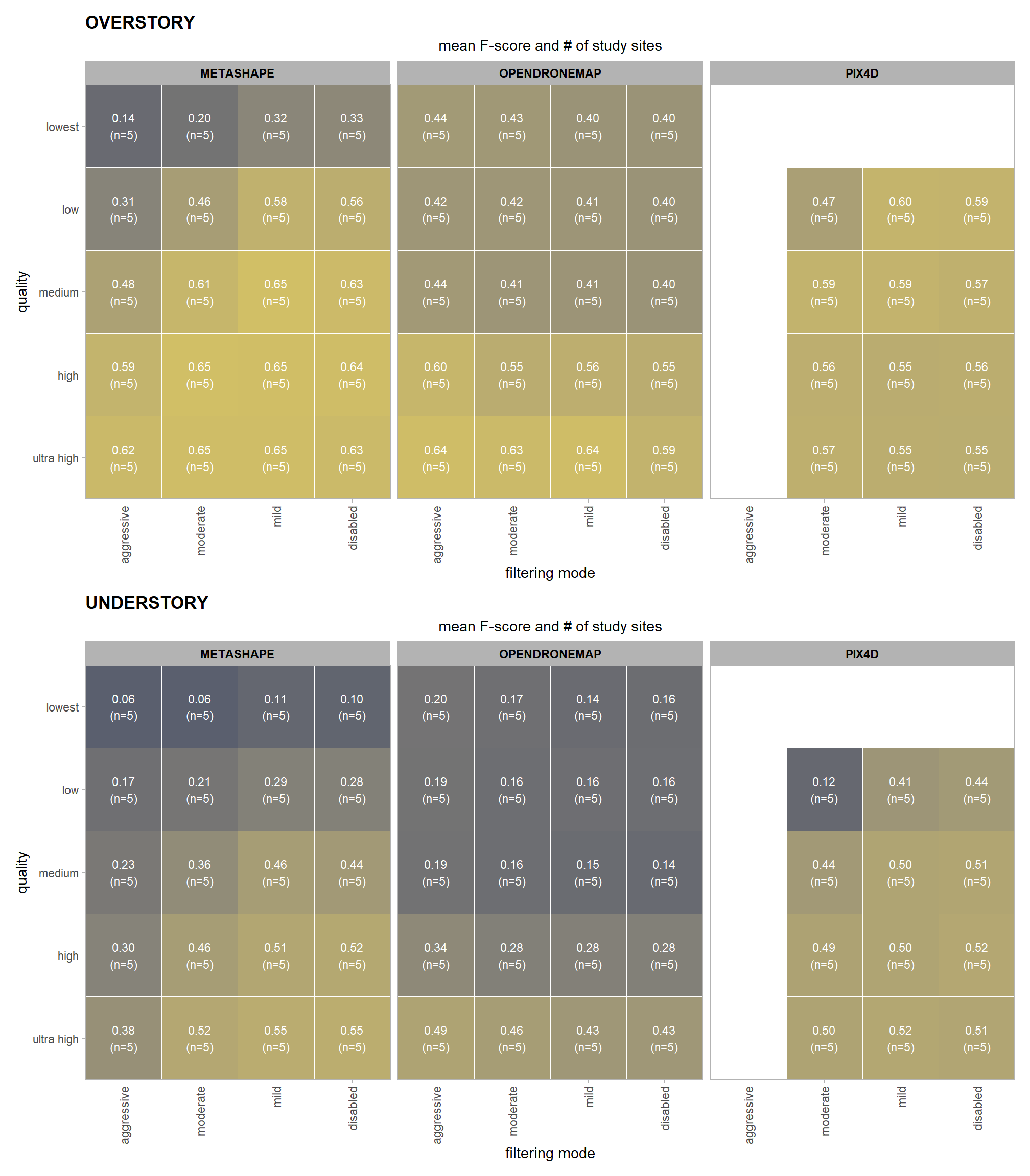
now let’s check by our other predictor variables
sum_stats_dta = function(my_var){
  sum_fns = list(
    n = ~sum(ifelse(is.na(.x), 0, 1))
    , min = ~min(.x, na.rm = TRUE)
    , max = ~max(.x, na.rm = TRUE)
    , mean = ~mean(.x, na.rm = TRUE)
    , median = ~median(.x, na.rm = TRUE)
    , sd = ~sd(.x, na.rm = TRUE)
  )
  # plot
  (
    ggplot(
      data = ou_ptcld_validation_data %>%
        dplyr::group_by(.data[[my_var]]) %>%
        dplyr::mutate(m = median(f_score))
      , mapping = aes(
        y = .data[[my_var]]
        , x = f_score, fill = m)
      ) +
      geom_violin(color = NA) +
      geom_boxplot(width = 0.1, outlier.shape = NA, fill = NA, color = "black") +
      geom_rug() +
      facet_grid(cols = vars(story)) +
      scale_fill_viridis_c(option = "mako", begin = 0.3, end = 0.9, direction = -1, limits = c(0,0.75)) +
      labs(
        x = "F-score"
        , y = stringr::str_replace_all(my_var, pattern = "_", replacement = " ")
        , subtitle = stringr::str_replace_all(my_var, pattern = "_", replacement = " ") %>%
          stringr::str_to_title()
      ) +
      theme_light() +
      theme(legend.position = "none", strip.text = element_text(color = "black", face = "bold"))
  )

}
# sum_stats_dta("software")
summarize for all variables of interest
c("software", "study_site"
  , "depth_maps_generation_quality"
  , "depth_maps_generation_filtering_mode"
) %>%
  purrr::map(sum_stats_dta)
## [[1]]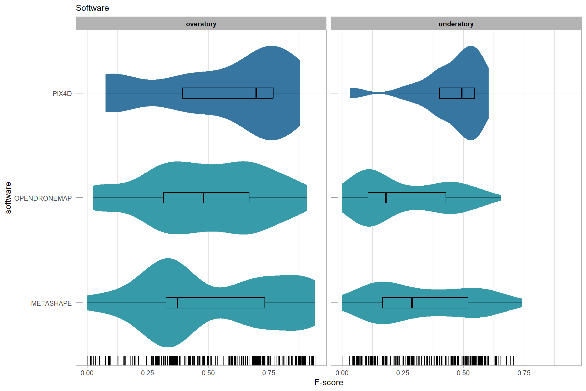
##
## [[2]]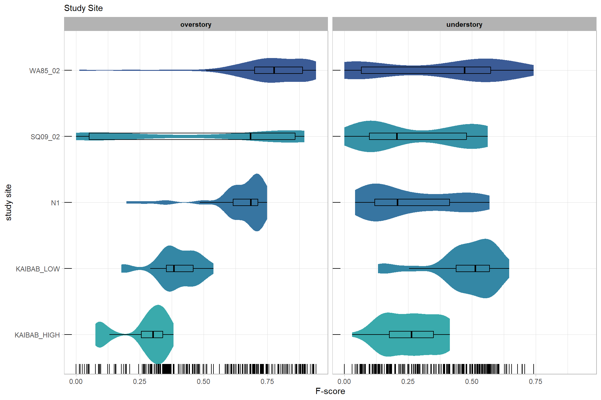
##
## [[3]]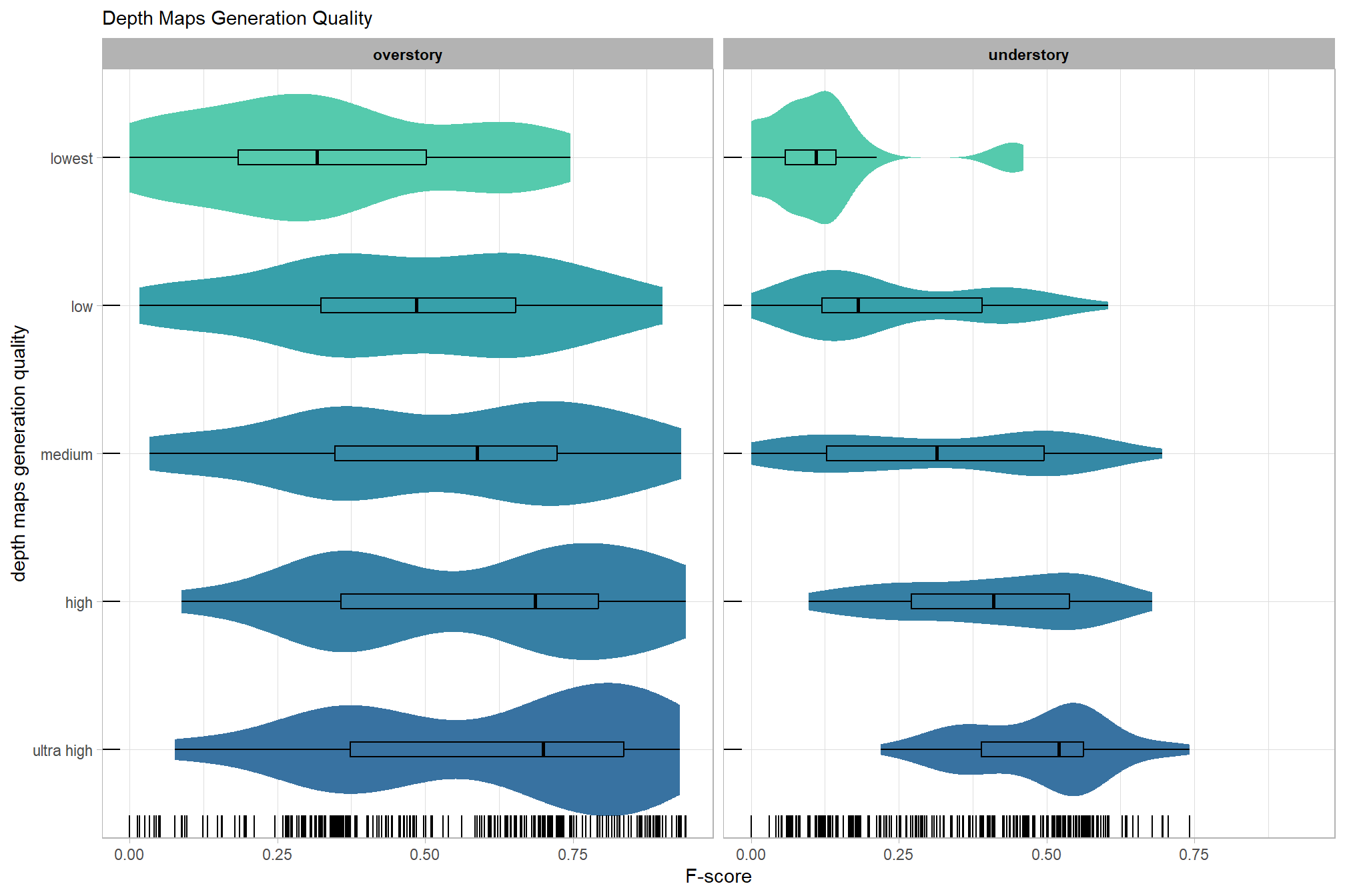
##
## [[4]]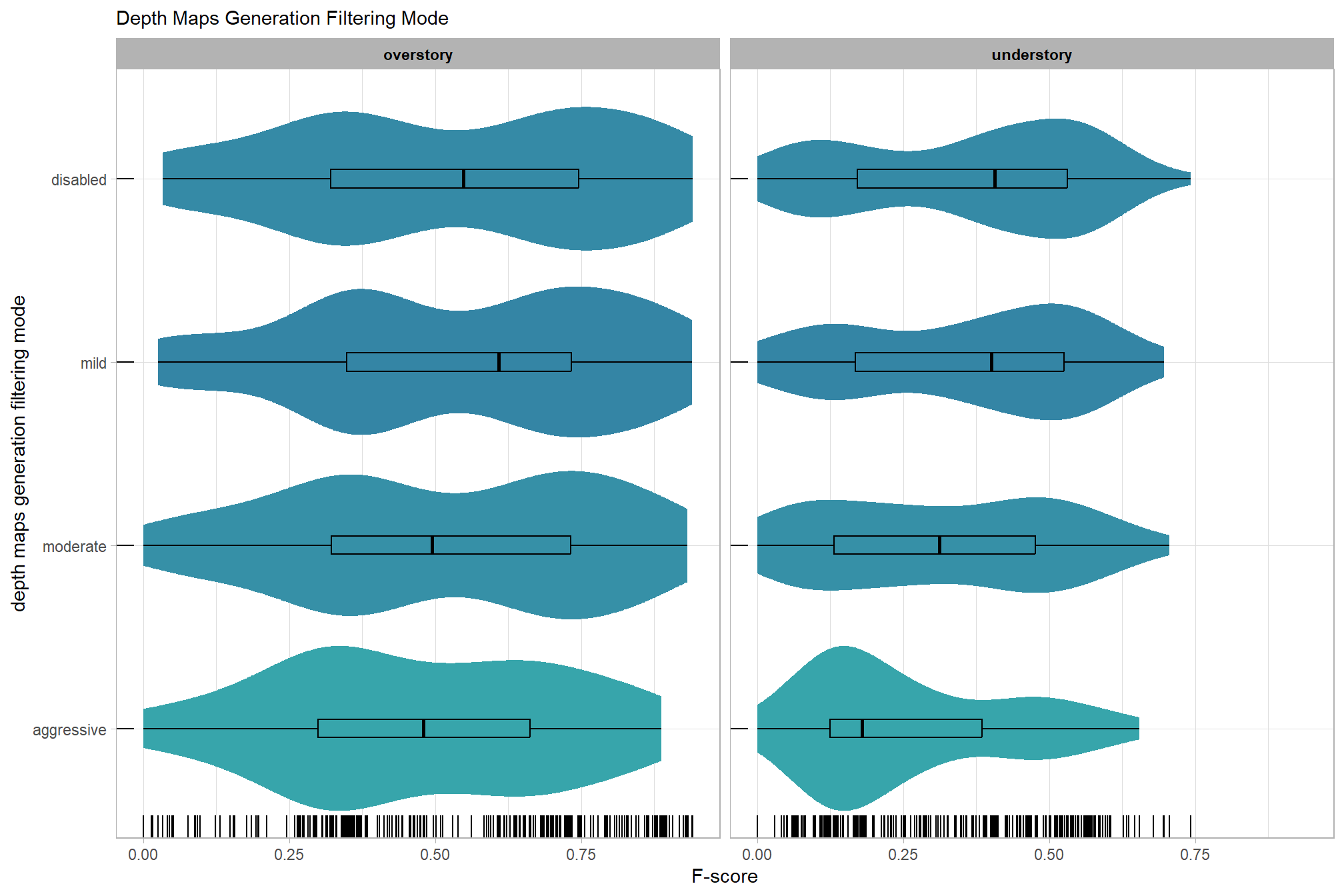
6.9.2 Bayesian
Need to check our prior selection…just go with brms defaults for now
Now fit the model.
brms_f_mod6 = brms::brm(
  formula = f_score ~
    # baseline
    1 +
    # main effects
    (1 | depth_maps_generation_quality) +
    (1 | depth_maps_generation_filtering_mode) +
    (1 | software) +
    (1 | story) +
    (1 | study_site) + # only fitting main effects of site and not interactions
    # two-way interactions
    (1 | depth_maps_generation_quality:depth_maps_generation_filtering_mode) +
    (1 | depth_maps_generation_quality:software) +
    (1 | depth_maps_generation_filtering_mode:software) +
    (1 | depth_maps_generation_quality:story) +
    (1 | depth_maps_generation_filtering_mode:story) +
    (1 | software:story) +
    # three-way interactions
    (1 | depth_maps_generation_quality:depth_maps_generation_filtering_mode:software) +
    (1 | depth_maps_generation_quality:depth_maps_generation_filtering_mode:story) +
    (1 | depth_maps_generation_quality:software:story) +
    (1 | depth_maps_generation_filtering_mode:software:story) +
    # four-way interactions
    (1 | depth_maps_generation_quality:depth_maps_generation_filtering_mode:software:story)
  , data = ou_ptcld_validation_data
  , family = Beta(link = "logit")
  , iter = 20000, warmup = 10000, chains = 4
  , control = list(adapt_delta = 0.999, max_treedepth = 13)
  , cores = round(parallel::detectCores()/2)
  , file = paste0(rootdir, "/fits/brms_f_mod6")
)
check the trace plots for problems with convergence of the Markov chains
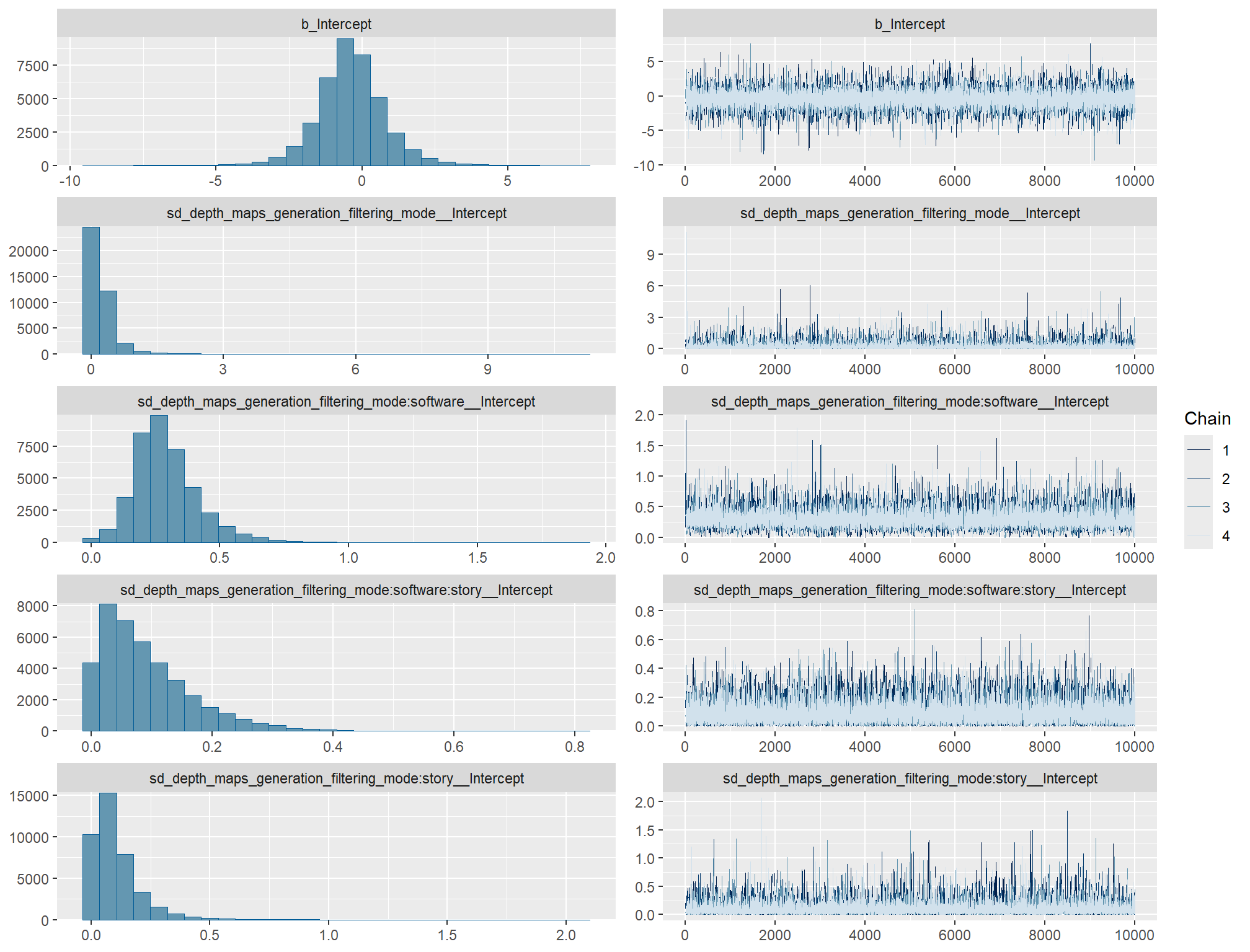
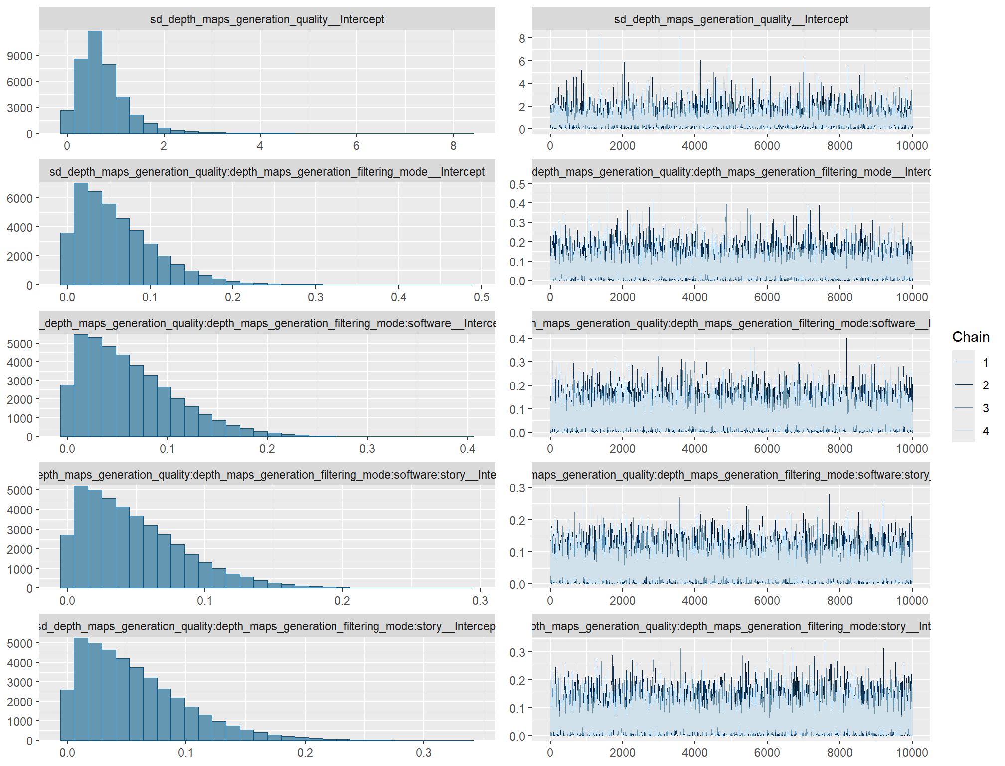
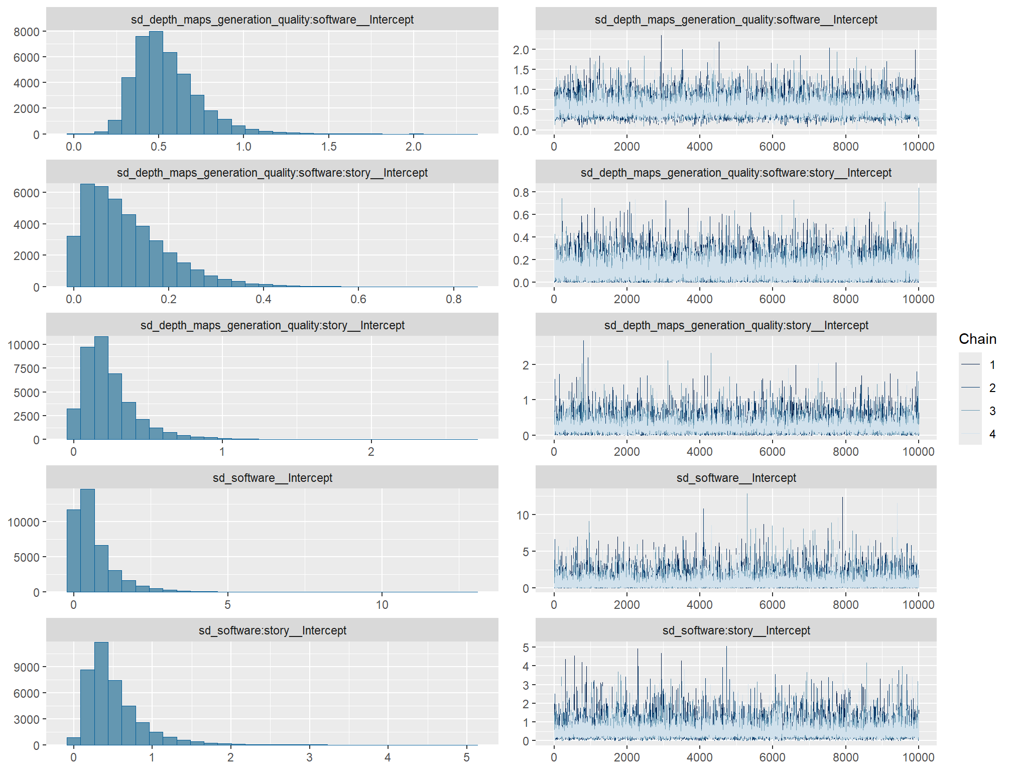
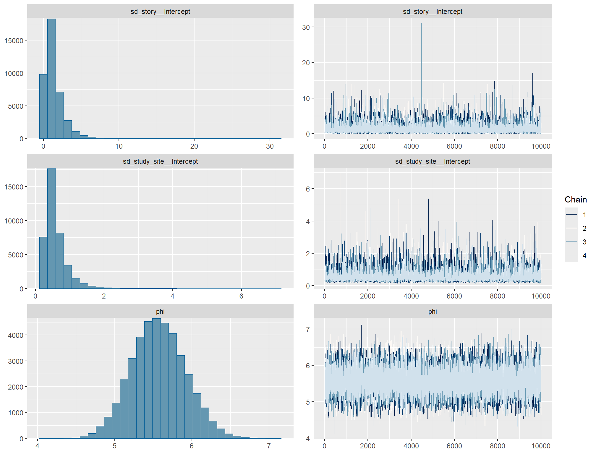
posterior-predictive check to make sure the model does an okay job simulating data that resemble the sample data
# posterior predictive check
brms::pp_check(
brms_f_mod6
, type = "dens_overlay"
, ndraws = 100
) +
labs(subtitle = "posterior-predictive check (overlaid densities)") +
theme_light() +
scale_y_continuous(NULL, breaks = NULL) +
theme(
legend.position = "top", legend.direction = "horizontal"
, legend.text = element_text(size = 14)
)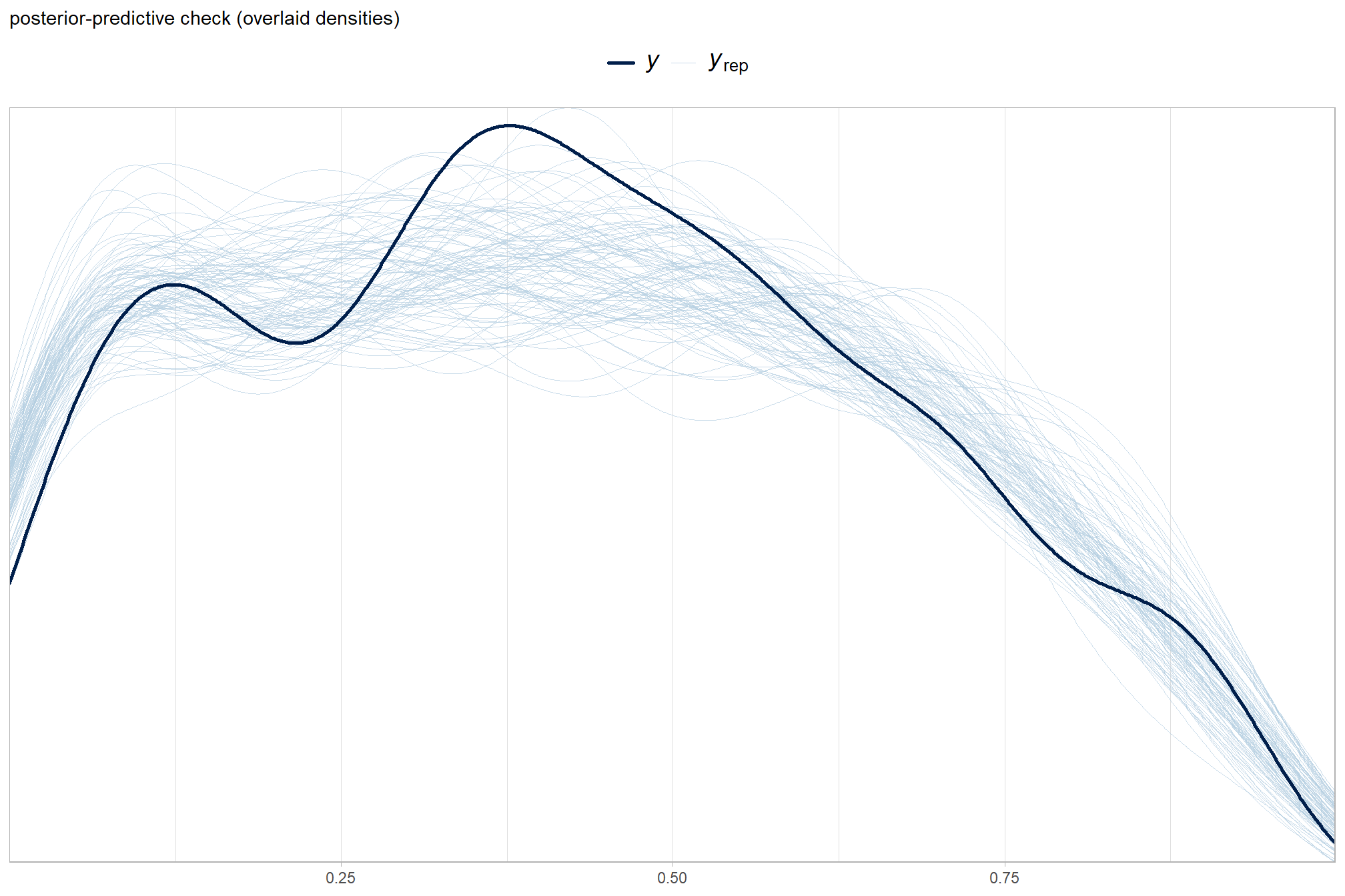
How’d we do capturing the conditional means and standard deviations by depth map generation quality?
# means
p1_temp = brms::pp_check(
brms_f_mod6
, type = "stat_grouped" # "dens_overlay_grouped"
, stat = "mean"
, group = "depth_maps_generation_quality"
) +
scale_y_continuous(NULL, breaks = c(NULL)) +
labs(subtitle = "means") +
facet_grid(cols = vars(group), scales = "free") +
theme_light()
# sds
p2_temp = brms::pp_check(
brms_f_mod6
, type = "stat_grouped" # "dens_overlay_grouped"
, stat = "sd"
, group = "depth_maps_generation_quality"
) +
scale_y_continuous(NULL, breaks = c(NULL)) +
labs(subtitle = "sd's") +
facet_grid(cols = vars(group), scales = "free") +
theme_light()
# combine
(p1_temp / p2_temp) &
theme(legend.position = "none") &
plot_annotation(
title = "Posterior-predictive statistical checks\nby dense cloud quality"
, subtitle = expression(
"The dark blue lines are "*italic(T(y))*", and the light blue bars are for "*italic(T)(italic(y)[rep])*".")
)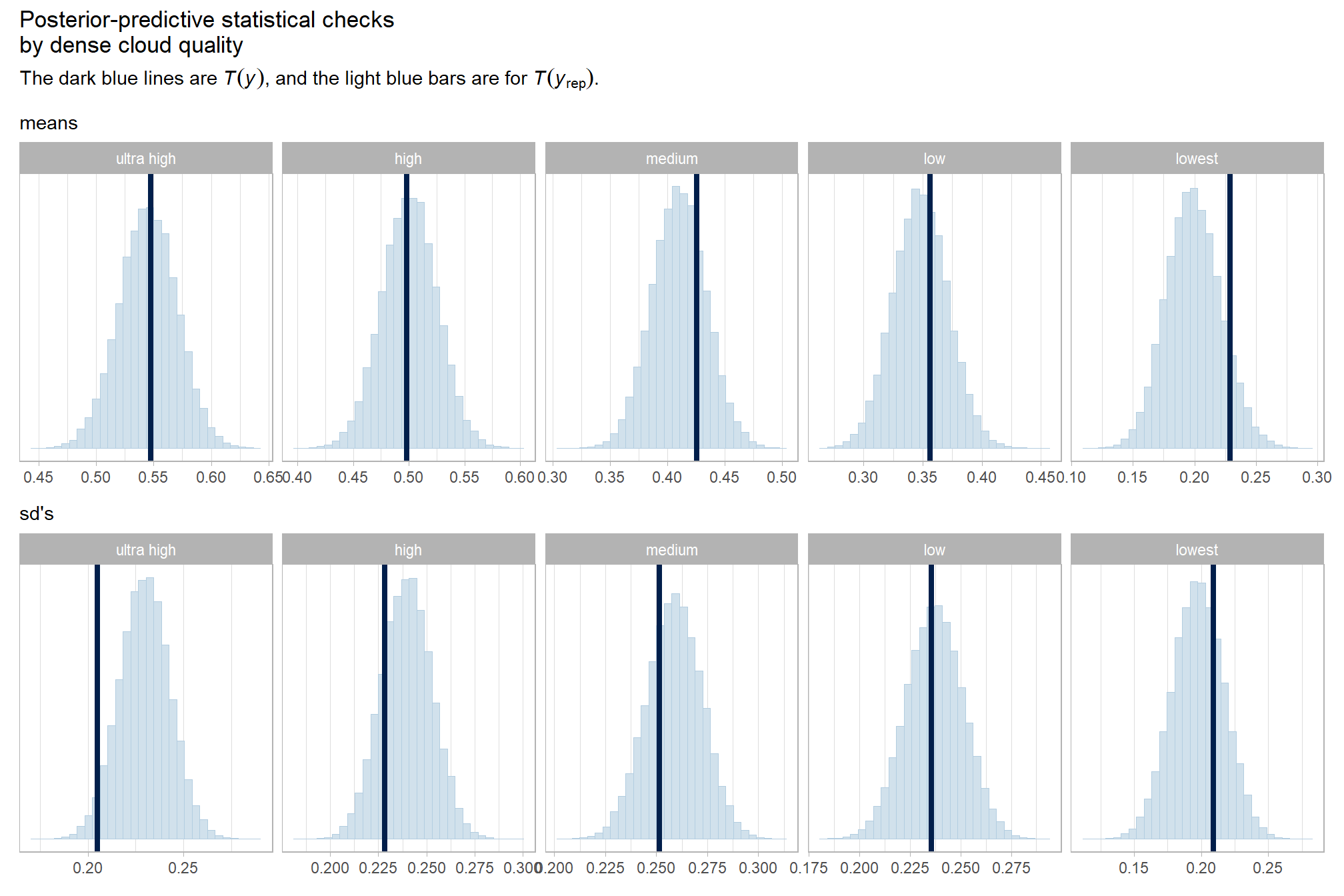
The means and sd’s of the F-score are less well represented across the different levels of dense cloud quality. We may want to look into modelling heterogeneous variances as shown by Kruschke chapter 20 and Kurz
What about for the software?
pp_check(brms_f_mod6, "dens_overlay_grouped", group = "software", ndraws = 100) +
labs(subtitle = "posterior-predictive check (overlaid densities)\nby software") +
theme_light() +
scale_y_continuous(NULL, breaks = NULL) +
theme(
legend.position = "top", legend.direction = "horizontal"
, legend.text = element_text(size = 14)
)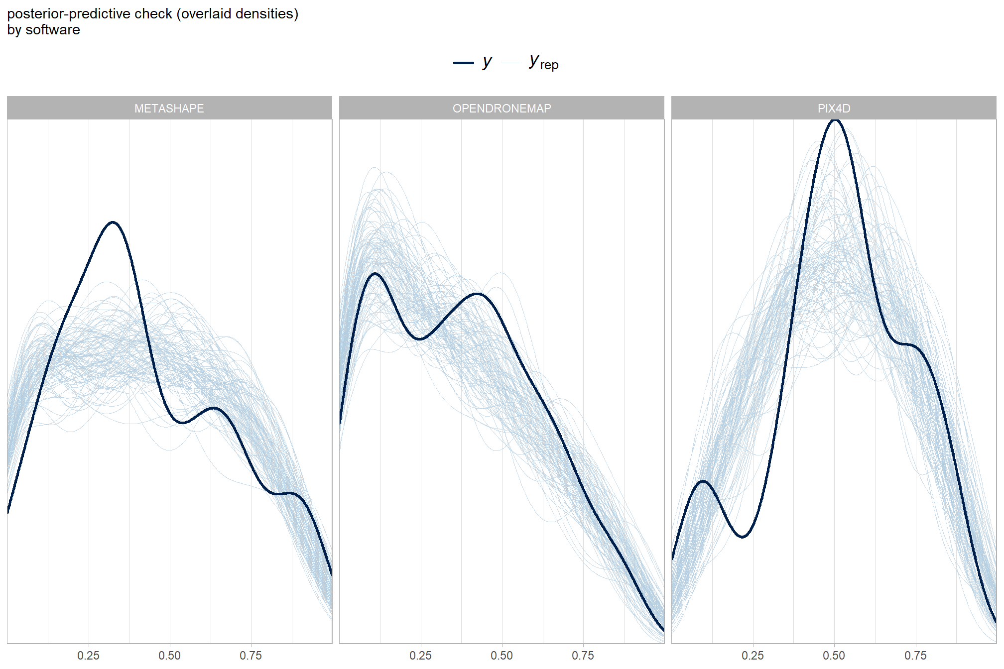
What about for the overstory/understory?
pp_check(brms_f_mod6, "dens_overlay_grouped", group = "story", ndraws = 100) +
labs(subtitle = "posterior-predictive check (overlaid densities)\nby story") +
theme_light() +
scale_y_continuous(NULL, breaks = NULL) +
theme(
legend.position = "top", legend.direction = "horizontal"
, legend.text = element_text(size = 14)
)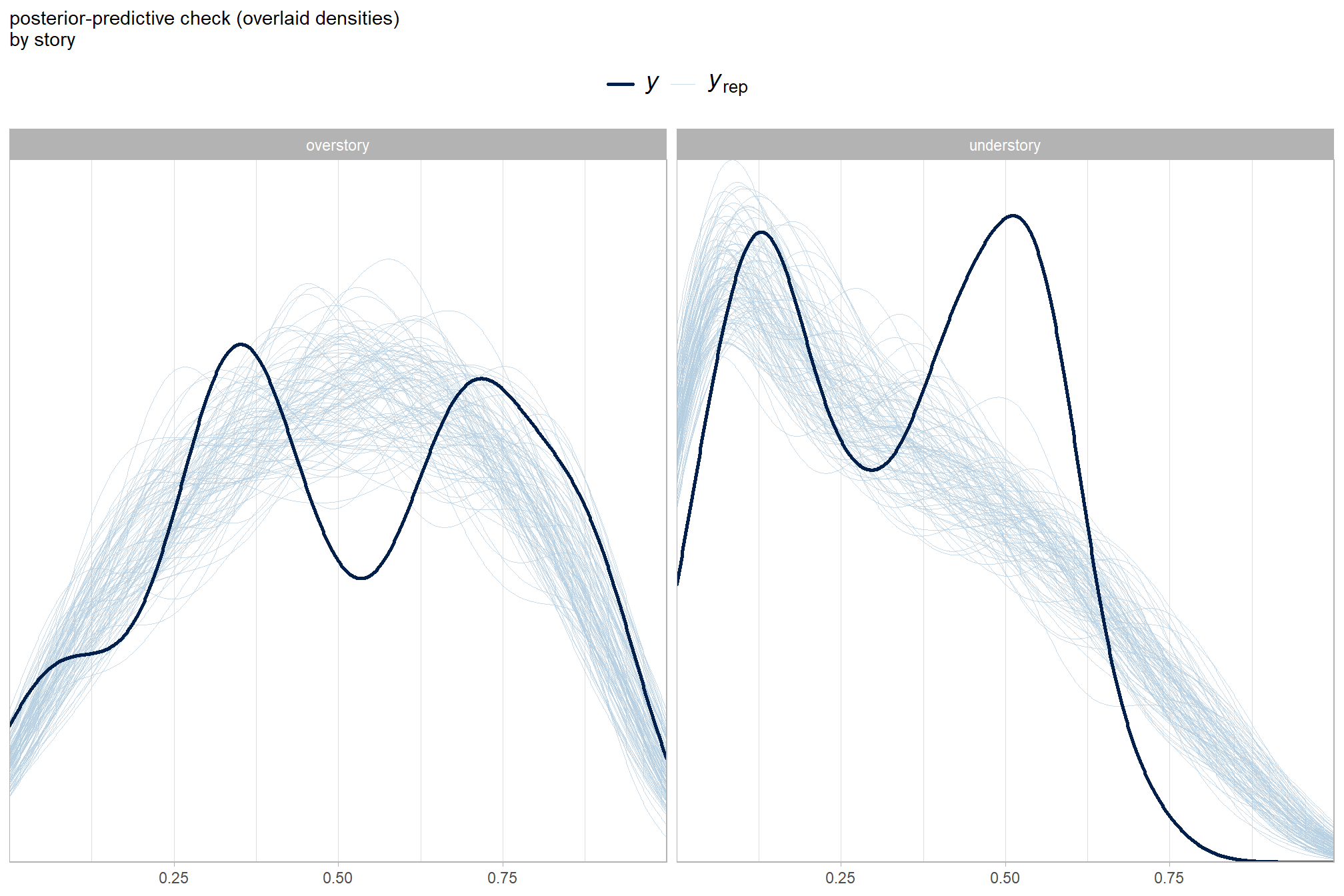
We may not be capturing the high versus low tree predictive performance that is being driven by differences at the study site level.
this should be addressed…is validation really that bad for some study sites?
We can look at the model noise standard deviation (concentration) \(\phi\).
# get formula
form_temp = brms_f_mod6$formula$formula[3] %>%
as.character() %>% get_frmla_text(split_chrs = 115) %>%
stringr::str_replace_all("depth_maps_generation_quality", "quality") %>%
stringr::str_replace_all("depth_maps_generation_filtering_mode", "filtering")
# extract the posterior draws
brms::as_draws_df(brms_f_mod6) %>%
# plot
ggplot(aes(x = phi, y = 0)) +
tidybayes::stat_dotsinterval(
point_interval = median_hdi, .width = .95
, justification = -0.04
, shape = 21, point_size = 3
, quantiles = 100
) +
scale_y_continuous(NULL, breaks = NULL) +
labs(
x = latex2exp::TeX("$\\phi$")
, caption = form_temp
) +
theme_light()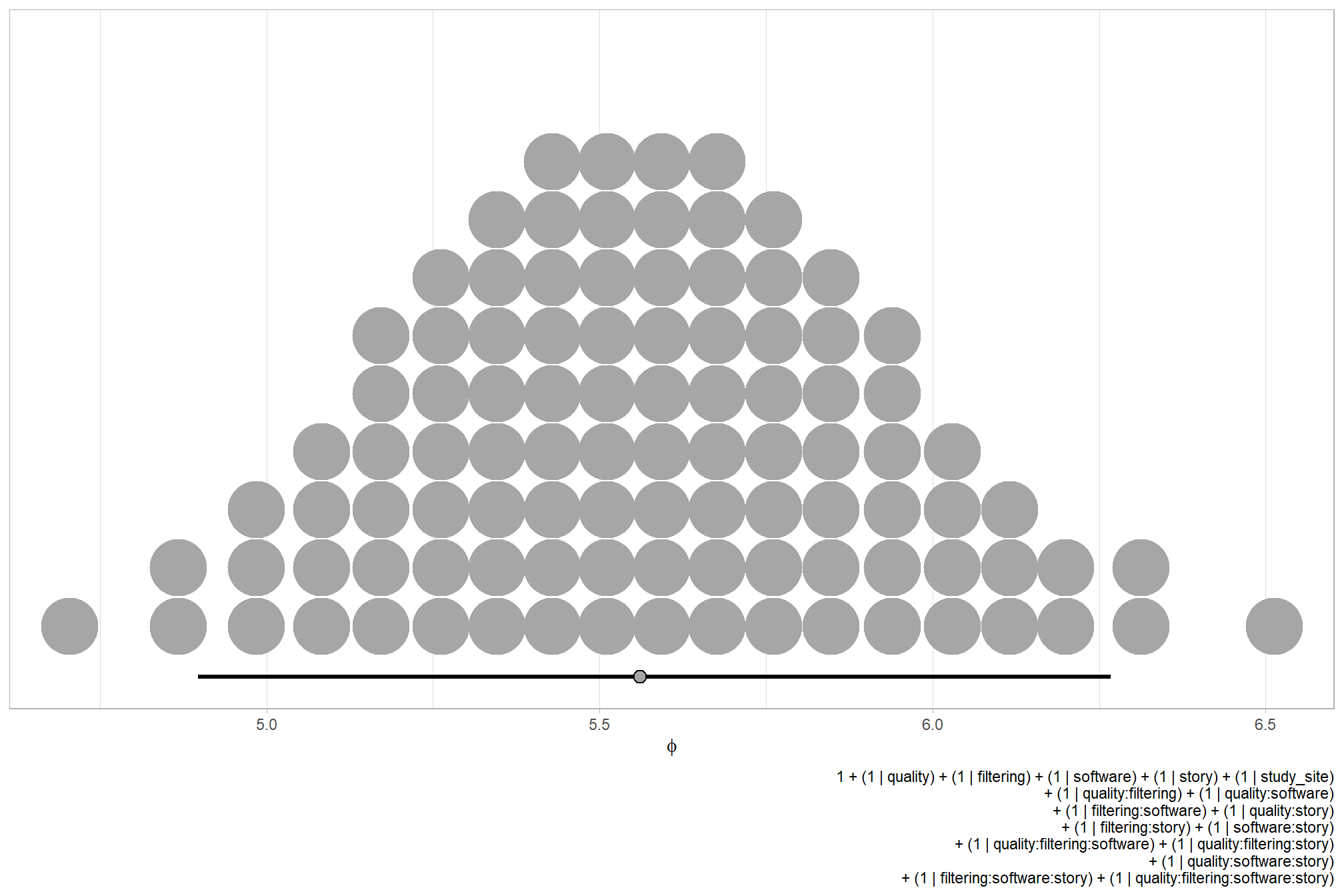
we can compare this to our beta model above without any overstory/understory predictor variable.
dplyr::bind_rows(
brms::as_draws_df(brms_f_mod6) %>% dplyr::select(phi) %>% dplyr::mutate(src = "brms_f_mod6")
, brms::as_draws_df(brms_f_mod5) %>% dplyr::select(phi) %>% dplyr::mutate(src = "brms_f_mod5")
) %>%
ggplot(mapping = aes(y = src, x = phi, color = src, group = src)) +
tidybayes::stat_pointinterval(position = "dodge") +
scale_y_discrete(NULL, breaks = NULL) +
scale_color_manual(values = viridis::turbo(n = 6, begin = 0.2, end = 0.8)[5:6]) +
labs(
y = "", x = latex2exp::TeX("$\\phi$")
, color = "model"
) +
theme_light() +
theme(legend.position = "top", strip.text = element_text(color = "black", face = "bold"))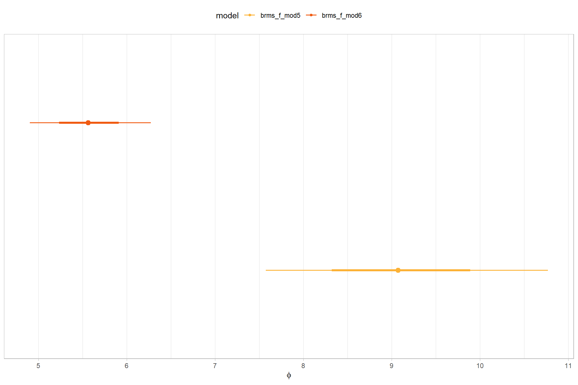
This indicates that our model including overstory/understory has less dispersion
6.9.2.1 Story - main effect
Now, we’ll look at the main effect of overstory/understory on F-score by collapsing across the filtering mode, dense cloud quality setting, study site, and software and then performing a pairwise comparison between overstory and understory
In a hierarchical model structure, we have to make use of the re_formula argument within tidybayes::add_epred_draws
ou_ptcld_validation_data %>%
dplyr::distinct(story) %>%
tidybayes::add_epred_draws(
brms_f_mod6, allow_new_levels = T
# this part is crucial
, re_formula = ~ (1 | story)
) %>%
dplyr::rename(value = .epred) %>%
# plot
ggplot(
mapping = aes(
x = value, y = story
, fill = story
)
) +
tidybayes::stat_halfeye(
point_interval = median_hdi, .width = .95
, interval_color = "gray66"
, shape = 21, point_color = "gray66", point_fill = "black"
, justification = -0.01
) +
scale_fill_viridis_d(option = "viridis", begin = 0.3, end = 0.7, drop = F) +
scale_x_continuous(breaks = scales::extended_breaks(n=8)) +
labs(
y = "", x = "F-score"
, subtitle = "posterior predictive distribution of F-score with 95% HDI"
, caption = form_temp
) +
theme_light() +
theme(legend.position = "none")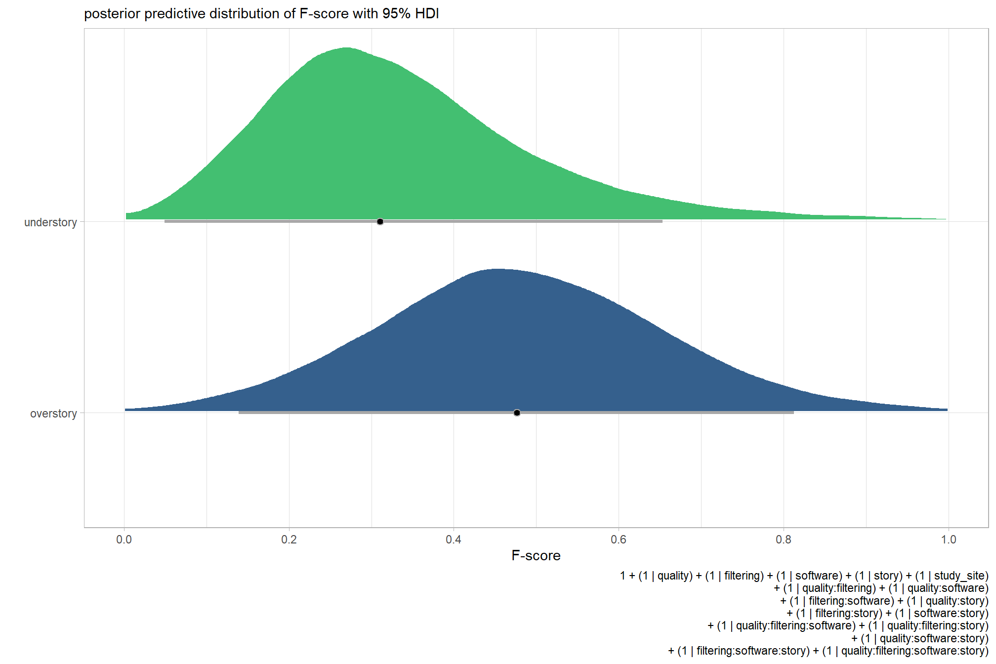
we can view the posterior HDI of these estimates
ou_ptcld_validation_data %>%
dplyr::distinct(story) %>%
tidybayes::add_epred_draws(
brms_f_mod6, allow_new_levels = T
# this part is crucial
, re_formula = ~ (1 | story)
) %>%
dplyr::rename(value = .epred) %>%
dplyr::group_by(story) %>%
tidybayes::median_hdi(value) %>%
select(-c(.point,.interval, .width)) %>%
kableExtra::kbl(
digits = 2
, caption = "brms::brm model: 95% HDI of the posterior predictive distribution of F-score"
, col.names = c(
""
, "F-score"
, "HDI low", "HDI high"
)
) %>%
kableExtra::kable_styling()| F-score | HDI low | HDI high | |
|---|---|---|---|
| overstory | 0.48 | 0.14 | 0.81 |
| understory | 0.31 | 0.05 | 0.65 |
compare this to the quick summary stats
ou_ptcld_validation_data %>%
dplyr::group_by(story) %>%
dplyr::summarise(
mean_f = mean(f_score)
, f_05 = quantile(f_score, probs = 0.05)
, f_95 = quantile(f_score, probs = 0.95)
) %>%
kableExtra::kbl(
digits = 2
, caption = "summary statistics of F-score"
, col.names = c(
""
, "mean F-score"
, "5% value", "95% value"
)
) %>%
kableExtra::kable_styling()| mean F-score | 5% value | 95% value | |
|---|---|---|---|
| overstory | 0.52 | 0.05 | 0.89 |
| understory | 0.33 | 0.04 | 0.60 |
now we’ll make our contrast of overstory/understory
brms_contrast_temp =
ou_ptcld_validation_data %>%
dplyr::distinct(story) %>%
tidybayes::add_epred_draws(
brms_f_mod6, allow_new_levels = T
# this part is crucial
, re_formula = ~ (1 | story)
) %>%
dplyr::rename(value = .epred) %>%
tidybayes::compare_levels(
value
, by = story
, comparison = tidybayes::emmeans_comparison("revpairwise")
) %>%
dplyr::rename(contrast = story) %>%
# median_hdi summary for coloring
dplyr::group_by(contrast) %>%
make_contrast_vars()
# what?
brms_contrast_temp %>% dplyr::glimpse()## Rows: 40,000
## Columns: 16
## Groups: contrast [1]
## $ .chain <int> NA, NA, NA, NA, NA, NA, NA, NA, NA, NA, NA, NA, NA, N…
## $ .iteration <int> NA, NA, NA, NA, NA, NA, NA, NA, NA, NA, NA, NA, NA, N…
## $ .draw <int> 1, 2, 3, 4, 5, 6, 7, 8, 9, 10, 11, 12, 13, 14, 15, 16…
## $ contrast <chr> "overstory - understory", "overstory - understory", "…
## $ value <dbl> 0.243671696, 0.196395881, 0.122113387, 0.187161358, 0…
## $ median_hdi_est <dbl> 0.1519276, 0.1519276, 0.1519276, 0.1519276, 0.1519276…
## $ median_hdi_lower <dbl> -0.06039082, -0.06039082, -0.06039082, -0.06039082, -…
## $ median_hdi_upper <dbl> 0.357243, 0.357243, 0.357243, 0.357243, 0.357243, 0.3…
## $ pr_gt_zero <chr> "92%", "92%", "92%", "92%", "92%", "92%", "92%", "92%…
## $ pr_lt_zero <chr> "8%", "8%", "8%", "8%", "8%", "8%", "8%", "8%", "8%",…
## $ is_diff_dir <lgl> TRUE, TRUE, TRUE, TRUE, TRUE, TRUE, TRUE, TRUE, FALSE…
## $ pr_diff <dbl> 0.918425, 0.918425, 0.918425, 0.918425, 0.918425, 0.9…
## $ pr_diff_lab <chr> "Pr(overstory>understory)=92%", "Pr(overstory>underst…
## $ pr_diff_lab_sm <chr> "Pr(>0)=92%", "Pr(>0)=92%", "Pr(>0)=92%", "Pr(>0)=92%…
## $ pr_diff_lab_pos <dbl> 0.3840362, 0.3840362, 0.3840362, 0.3840362, 0.3840362…
## $ sig_level <ord> 90%, 90%, 90%, 90%, 90%, 90%, 90%, 90%, 90%, 90%, 90%…plot it
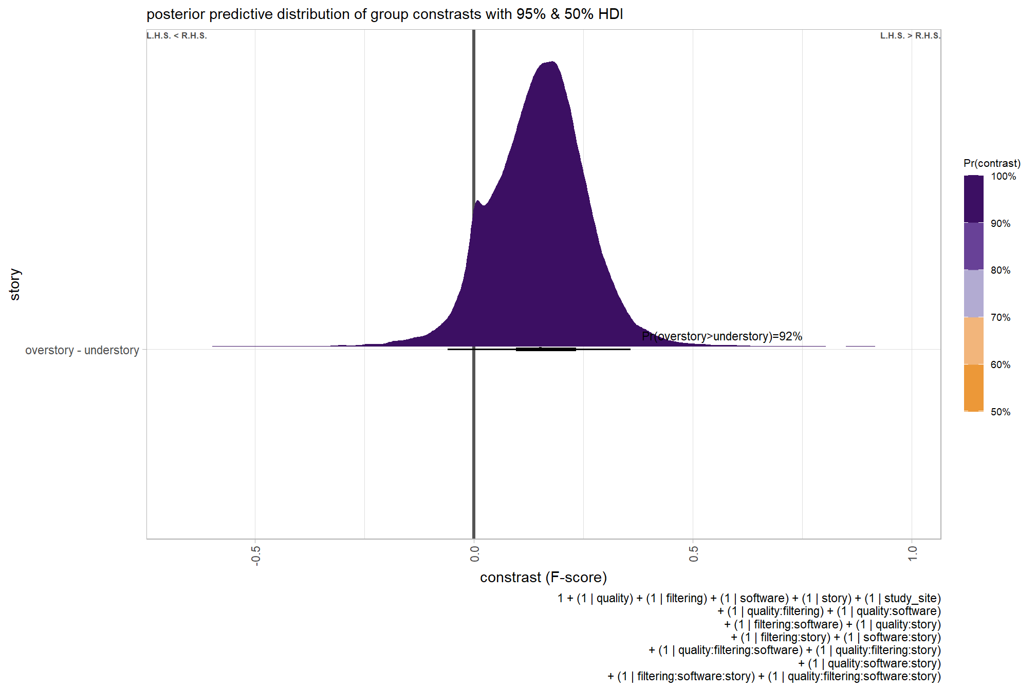
ggplot2::ggsave(
"../data/stry_comp_mod6.png"
, plot = ggplot2::last_plot() + labs(subtitle = "")
, height = 7, width = 10.5
)and summarize these contrasts
brms_contrast_temp %>%
dplyr::group_by(contrast, pr_gt_zero) %>%
tidybayes::median_hdi(value) %>%
dplyr::arrange(contrast) %>%
dplyr::select(contrast, value, .lower, .upper, pr_gt_zero) %>%
kableExtra::kbl(
digits = 2
, caption = "brms::brm model: 95% HDI of the posterior predictive distribution of group constrasts"
, col.names = c(
"overstory contrast"
, "difference (F-score)"
, "HDI low", "HDI high"
, "Pr(diff>0)"
)
) %>%
kableExtra::kable_styling()| overstory contrast | difference (F-score) | HDI low | HDI high | Pr(diff>0) |
|---|---|---|---|---|
| overstory - understory | 0.15 | -0.06 | 0.36 | 92% |
Averaging across all levels of filtering mode, dense cloud quality setting, study site, and software the process does a better job detecting overstory trees than understory trees. Because this is a Bayesian analysis we can quantify this probability: there is a 91.8% that overstory trees will be detected with better accuracy than understory trees (see coloring on posterior predictive distribution above)
6.9.2.2 Story:Software - interaction
Now, we’ll address the question of “are there differences in F-score based on the processing software used for detecting overstory and understory trees?”
# get draws
stry_sftwr_draws_temp = ou_ptcld_validation_data %>%
dplyr::distinct(software, story) %>%
tidybayes::add_epred_draws(
brms_f_mod6, allow_new_levels = T
# this part is crucial
, re_formula = ~ (1 | story) +
(1 | software) +
(1 | software:story)
) %>%
dplyr::rename(value = .epred)
# calculate contrast
brms_contrast_temp = stry_sftwr_draws_temp %>%
tidybayes::compare_levels(
value
, by = software
, comparison = "pairwise"
) %>%
dplyr::rename(contrast = software) %>%
# median_hdi summary for coloring
dplyr::group_by(contrast, story) %>%
make_contrast_vars()
# what?
brms_contrast_temp %>% dplyr::glimpse()## Rows: 240,000
## Columns: 17
## Groups: contrast, story [6]
## $ story <fct> overstory, overstory, overstory, overstory, overstory…
## $ .chain <int> NA, NA, NA, NA, NA, NA, NA, NA, NA, NA, NA, NA, NA, N…
## $ .iteration <int> NA, NA, NA, NA, NA, NA, NA, NA, NA, NA, NA, NA, NA, N…
## $ .draw <int> 1, 2, 3, 4, 5, 6, 7, 8, 9, 10, 11, 12, 13, 14, 15, 16…
## $ contrast <chr> "OPENDRONEMAP - METASHAPE", "OPENDRONEMAP - METASHAPE…
## $ value <dbl> -0.023445297, 0.029402995, 0.041254983, -0.010283702,…
## $ median_hdi_est <dbl> -0.01381908, -0.01381908, -0.01381908, -0.01381908, -…
## $ median_hdi_lower <dbl> -0.2029299, -0.2029299, -0.2029299, -0.2029299, -0.20…
## $ median_hdi_upper <dbl> 0.1648562, 0.1648562, 0.1648562, 0.1648562, 0.1648562…
## $ pr_gt_zero <chr> "43%", "43%", "43%", "43%", "43%", "43%", "43%", "43%…
## $ pr_lt_zero <chr> "57%", "57%", "57%", "57%", "57%", "57%", "57%", "57%…
## $ is_diff_dir <lgl> TRUE, FALSE, FALSE, TRUE, TRUE, FALSE, TRUE, TRUE, FA…
## $ pr_diff <dbl> 0.567825, 0.567825, 0.567825, 0.567825, 0.567825, 0.5…
## $ pr_diff_lab <chr> "Pr(MtaShp>ODM)=57%", "Pr(MtaShp>ODM)=57%", "Pr(MtaSh…
## $ pr_diff_lab_sm <chr> "Pr(<0)=57%", "Pr(<0)=57%", "Pr(<0)=57%", "Pr(<0)=57%…
## $ pr_diff_lab_pos <dbl> -0.2181497, -0.2181497, -0.2181497, -0.2181497, -0.21…
## $ sig_level <ord> <80%, <80%, <80%, <80%, <80%, <80%, <80%, <80%, <80%,…plot it
plt_contrast(
brms_contrast_temp, caption_text = form_temp
, y_axis_title = "software"
, facet = "story"
, label_size = 2.5
, x_expand = c(0.17,0.3)
) +
labs(
subtitle = "posterior predictive distribution of group constrasts with 95% & 50% HDI\nby overstory/understory"
)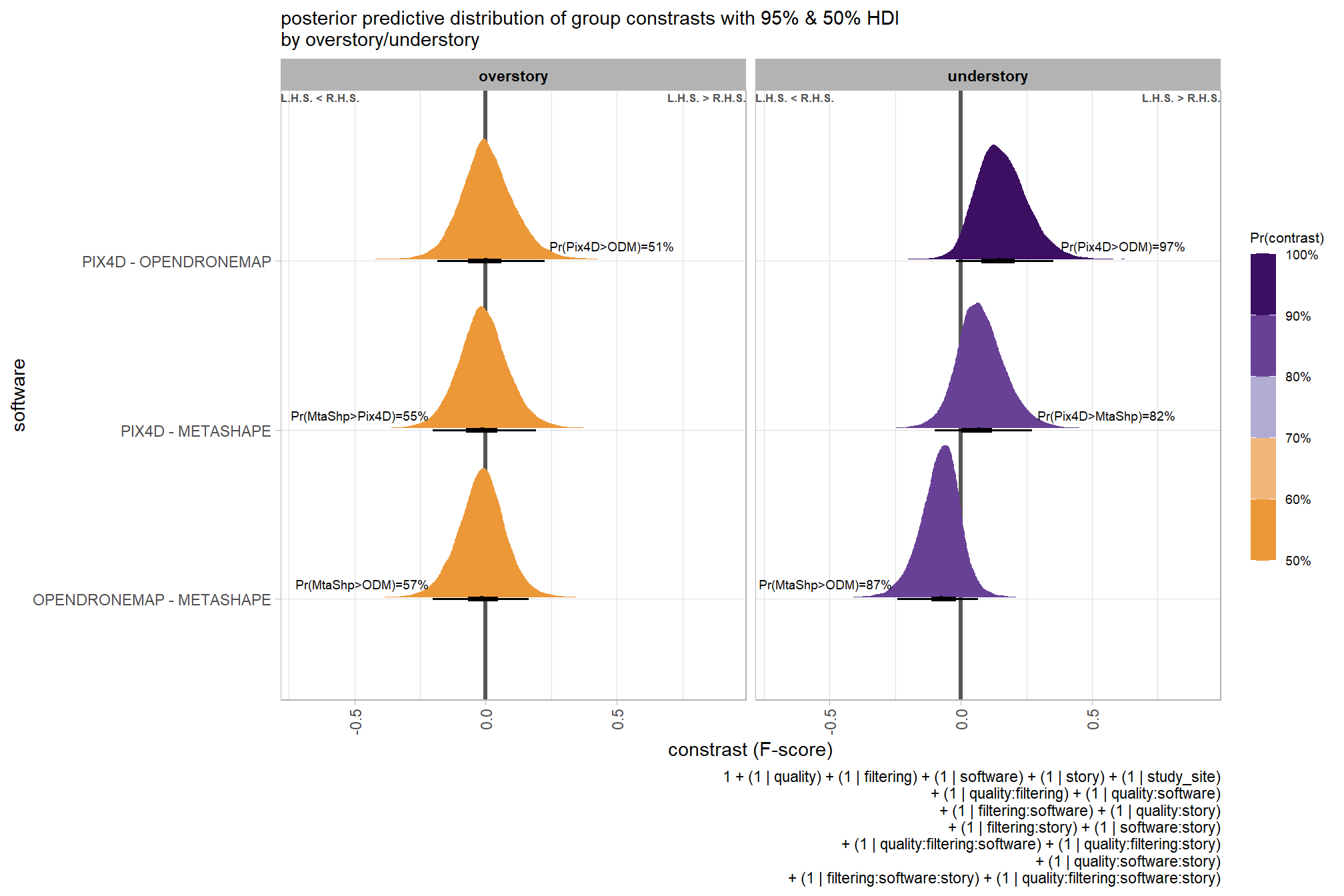
ggplot2::ggsave(
"../data/sftwr_stry_comp_mod6.png"
, plot = ggplot2::last_plot() + labs(subtitle = "")
, height = 7, width = 10.5
)and summarize these contrasts
brms_contrast_temp %>%
dplyr::group_by(contrast, story, pr_gt_zero) %>%
tidybayes::median_hdi(value) %>%
dplyr::arrange(contrast, story) %>%
dplyr::select(contrast, story, value, .lower, .upper, pr_gt_zero) %>%
kableExtra::kbl(
digits = 2
, caption = "brms::brm model: 95% HDI of the posterior predictive distribution of group constrasts"
, col.names = c(
"software contrast"
, "overstory/understory"
, "difference (F-score)"
, "HDI low", "HDI high"
, "Pr(diff>0)"
)
) %>%
kableExtra::kable_styling()| software contrast | overstory/understory | difference (F-score) | HDI low | HDI high | Pr(diff>0) |
|---|---|---|---|---|---|
| OPENDRONEMAP - METASHAPE | overstory | -0.01 | -0.20 | 0.16 | 43% |
| OPENDRONEMAP - METASHAPE | understory | -0.07 | -0.24 | 0.06 | 13% |
| PIX4D - METASHAPE | overstory | -0.01 | -0.20 | 0.19 | 45% |
| PIX4D - METASHAPE | understory | 0.07 | -0.10 | 0.27 | 82% |
| PIX4D - OPENDRONEMAP | overstory | 0.00 | -0.18 | 0.23 | 51% |
| PIX4D - OPENDRONEMAP | understory | 0.15 | -0.02 | 0.35 | 97% |
6.9.2.3 Story:Quality - interaction
What is the difference in F-score between overstory and understory for the different levels of dense cloud quality?
Note that how within tidybayes::add_epred_draws, we used the re_formula argument to average over the effects of study site, software, and filtering mode to compare the dense cloud quality and story effects.
ou_ptcld_validation_data %>%
dplyr::distinct(depth_maps_generation_quality, story) %>%
tidybayes::add_epred_draws(
brms_f_mod6, allow_new_levels = T
# this part is crucial
, re_formula = ~ (1 | depth_maps_generation_quality) +
(1 | story) +
(1 | depth_maps_generation_quality:story)
) %>%
dplyr::rename(value = .epred) %>%
dplyr::mutate(depth_maps_generation_quality = depth_maps_generation_quality %>% forcats::fct_rev()) %>%
# plot
ggplot(
mapping = aes(
y = value, x = story
, fill = story
)
) +
tidybayes::stat_eye(
point_interval = median_hdi, .width = .95
, slab_alpha = 0.8
, interval_color = "black", linewidth = 1
, point_color = "black", point_fill = "black", point_size = 1
) +
scale_fill_viridis_d(option = "viridis", begin = 0.3, end = 0.7, drop = F) +
scale_y_continuous(breaks = scales::extended_breaks(n=10)) +
facet_grid(cols = vars(depth_maps_generation_quality)) +
labs(
x = "story", y = "F-score"
, subtitle = "posterior predictive distribution of F-score with 95% HDI\nby dense cloud quality"
, caption = form_temp
) +
theme_light() +
theme(
legend.position = "none"
, legend.direction = "horizontal"
, axis.text.x = element_text(angle = 90, vjust = 0.5, hjust = 1)
, strip.text = element_text(color = "black", face = "bold")
) 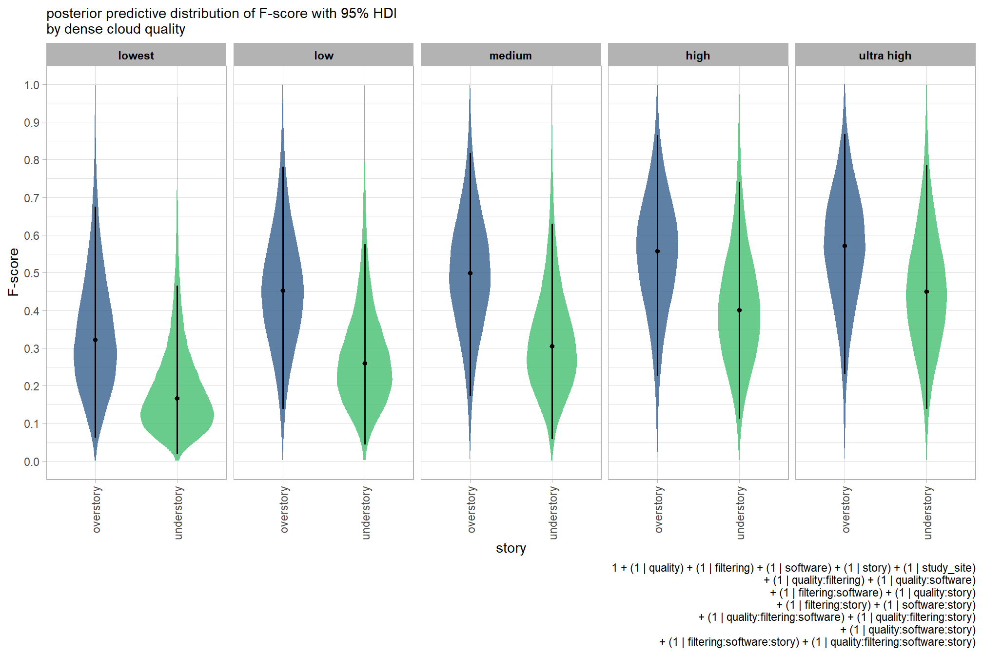
6.9.2.4 Quality:Filtering - interaction
Are there differences in F-score based on dense point cloud generation quality within each level of filtering mode?
Here, we collapse across the study site, software, and story to compare the combined dense cloud quality and filtering mode effect.
In a hierarchical model structure, we have to make use of the re_formula argument within tidybayes::add_epred_draws
qlty_filter_draws_temp =
ptcld_validation_data %>%
dplyr::distinct(depth_maps_generation_quality, depth_maps_generation_filtering_mode) %>%
tidybayes::add_epred_draws(
brms_f_mod6, allow_new_levels = T
# this part is crucial
, re_formula = ~ (1 | depth_maps_generation_quality) +
(1 | depth_maps_generation_filtering_mode) +
(1 | depth_maps_generation_quality:depth_maps_generation_filtering_mode)
) %>%
dplyr::rename(value = .epred)
# plot
qlty_filter_draws_temp %>%
dplyr::mutate(depth_maps_generation_quality = depth_maps_generation_quality %>% forcats::fct_rev()) %>%
# plot
ggplot(
mapping = aes(
y = value, x = depth_maps_generation_filtering_mode
, fill = depth_maps_generation_filtering_mode
)
) +
tidybayes::stat_eye(
point_interval = median_hdi, .width = .95
, slab_alpha = 0.8
, interval_color = "black", linewidth = 1
, point_color = "black", point_fill = "black", point_size = 1
) +
scale_fill_viridis_d(option = "plasma", drop = F) +
scale_y_continuous(breaks = scales::extended_breaks(n=10)) +
facet_grid(cols = vars(depth_maps_generation_quality)) +
labs(
x = "filtering mode", y = "F-score"
, subtitle = "posterior predictive distribution of F-score with 95% HDI\nby dense cloud quality"
, fill = "Filtering Mode"
, caption = form_temp
) +
theme_light() +
theme(
legend.position = "none"
, legend.direction = "horizontal"
, axis.text.x = element_text(angle = 90, vjust = 0.5, hjust = 1)
, strip.text = element_text(color = "black", face = "bold")
) 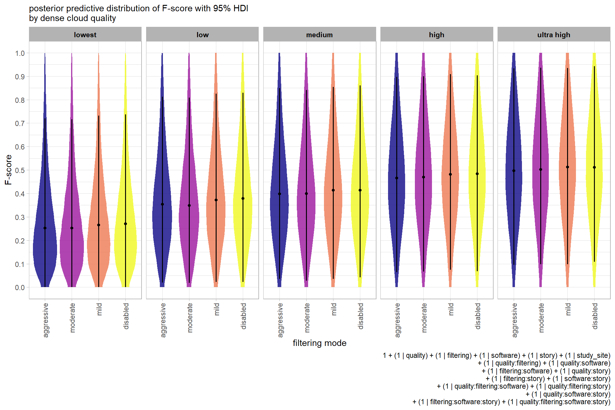
ggplot2::ggsave(
"../data/qlty_fltr_mod6.png"
, plot = ggplot2::last_plot() + labs(subtitle = "")
, height = 7, width = 10.5
)we can also make pairwise comparisons so long as we continue using tidybayes::add_epred_draws with the re_formula argument
brms_contrast_temp = qlty_filter_draws_temp %>%
tidybayes::compare_levels(
value
, by = depth_maps_generation_quality
, comparison =
contrast_list
# tidybayes::emmeans_comparison("revpairwise")
#"pairwise"
) %>%
dplyr::rename(contrast = depth_maps_generation_quality)
# separate contrast
brms_contrast_temp = brms_contrast_temp %>%
dplyr::ungroup() %>%
tidyr::separate_wider_delim(
cols = contrast
, delim = " - "
, names = paste0(
"sorter"
, 1:(max(stringr::str_count(brms_contrast_temp$contrast, "-"))+1)
)
, too_few = "align_start"
, cols_remove = F
) %>%
dplyr::filter(sorter1!=sorter2) %>%
dplyr::mutate(
dplyr::across(
tidyselect::starts_with("sorter")
, .fns = function(x){factor(
x, ordered = T
, levels = levels(ptcld_validation_data$depth_maps_generation_quality)
)}
)
, contrast = contrast %>%
forcats::fct_reorder(
paste0(as.numeric(sorter1), as.numeric(sorter2)) %>%
as.numeric()
)
, depth_maps_generation_filtering_mode = depth_maps_generation_filtering_mode %>%
factor(
levels = levels(ptcld_validation_data$depth_maps_generation_filtering_mode)
, ordered = T
)
) %>%
# median_hdi summary for coloring
dplyr::group_by(contrast,depth_maps_generation_filtering_mode) %>%
make_contrast_vars()
# what?
brms_contrast_temp %>% dplyr::glimpse()## Rows: 1,600,000
## Columns: 19
## Groups: contrast, depth_maps_generation_filtering_mode [40]
## $ depth_maps_generation_filtering_mode <ord> aggressive, aggressive, aggressiv…
## $ .chain <int> NA, NA, NA, NA, NA, NA, NA, NA, N…
## $ .iteration <int> NA, NA, NA, NA, NA, NA, NA, NA, N…
## $ .draw <int> 1, 2, 3, 4, 5, 6, 7, 8, 9, 10, 11…
## $ sorter1 <ord> ultra high, ultra high, ultra hig…
## $ sorter2 <ord> high, high, high, high, high, hig…
## $ contrast <fct> ultra high - high, ultra high - h…
## $ value <dbl> 0.069614286, 0.040784609, -0.0046…
## $ median_hdi_est <dbl> 0.01972114, 0.01972114, 0.0197211…
## $ median_hdi_lower <dbl> -0.160384, -0.160384, -0.160384, …
## $ median_hdi_upper <dbl> 0.2231248, 0.2231248, 0.2231248, …
## $ pr_gt_zero <chr> "62%", "62%", "62%", "62%", "62%"…
## $ pr_lt_zero <chr> "38%", "38%", "38%", "38%", "38%"…
## $ is_diff_dir <lgl> TRUE, TRUE, FALSE, TRUE, FALSE, T…
## $ pr_diff <dbl> 0.6208, 0.6208, 0.6208, 0.6208, 0…
## $ pr_diff_lab <chr> "Pr(ultra high>high)=62%", "Pr(ul…
## $ pr_diff_lab_sm <chr> "Pr(>0)=62%", "Pr(>0)=62%", "Pr(>…
## $ pr_diff_lab_pos <dbl> 0.2398591, 0.2398591, 0.2398591, …
## $ sig_level <ord> <80%, <80%, <80%, <80%, <80%, <80…plot it
plt_contrast(
brms_contrast_temp, caption_text = form_temp
, y_axis_title = "quality"
, facet = "depth_maps_generation_filtering_mode"
, label_size = 2.0
, x_expand = c(0,0.6)
) +
labs(
subtitle = "posterior predictive distribution of group constrasts with 95% & 50% HDI\nby filtering mode"
) +
theme(
axis.text.x = element_text(size = 7)
)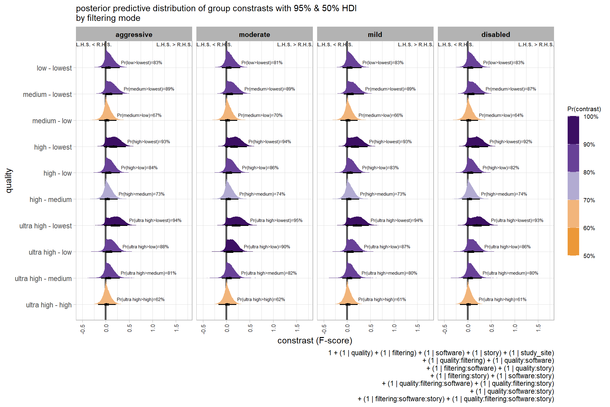
ggplot2::ggsave(
"../data/qlty_fltr_comp_mod6.png"
, plot = ggplot2::last_plot() + labs(subtitle = "")
, height = 7, width = 10.5
)and summarize these contrasts
brms_contrast_temp %>%
dplyr::group_by(contrast, depth_maps_generation_filtering_mode, pr_gt_zero) %>%
tidybayes::median_hdi(value) %>%
dplyr::arrange(contrast, depth_maps_generation_filtering_mode) %>%
dplyr::select(contrast, depth_maps_generation_filtering_mode, value, .lower, .upper, pr_gt_zero) %>%
kableExtra::kbl(
digits = 2
, caption = "brms::brm model: 95% HDI of the posterior predictive distribution of group constrasts"
, col.names = c(
"quality contrast"
, "filtering mode"
, "difference (F-score)"
, "HDI low", "HDI high"
, "Pr(diff>0)"
)
) %>%
kableExtra::kable_styling() %>%
kableExtra::scroll_box(height = "8in")| quality contrast | filtering mode | difference (F-score) | HDI low | HDI high | Pr(diff>0) |
|---|---|---|---|---|---|
| ultra high - high | aggressive | 0.02 | -0.16 | 0.22 | 62% |
| ultra high - high | aggressive | 0.02 | 0.22 | 0.22 | 62% |
| ultra high - high | moderate | 0.02 | -0.17 | 0.22 | 62% |
| ultra high - high | mild | 0.02 | -0.15 | 0.22 | 61% |
| ultra high - high | disabled | 0.02 | -0.16 | 0.22 | 61% |
| ultra high - medium | aggressive | 0.07 | -0.10 | 0.30 | 81% |
| ultra high - medium | moderate | 0.07 | -0.10 | 0.29 | 82% |
| ultra high - medium | mild | 0.07 | -0.10 | 0.29 | 80% |
| ultra high - medium | disabled | 0.07 | -0.10 | 0.30 | 80% |
| ultra high - low | aggressive | 0.11 | -0.07 | 0.34 | 88% |
| ultra high - low | moderate | 0.12 | -0.06 | 0.35 | 90% |
| ultra high - low | mild | 0.11 | -0.07 | 0.34 | 87% |
| ultra high - low | disabled | 0.10 | -0.08 | 0.33 | 86% |
| ultra high - lowest | aggressive | 0.20 | -0.04 | 0.47 | 94% |
| ultra high - lowest | moderate | 0.20 | -0.03 | 0.47 | 95% |
| ultra high - lowest | mild | 0.20 | -0.03 | 0.47 | 94% |
| ultra high - lowest | disabled | 0.20 | -0.04 | 0.47 | 93% |
| high - medium | aggressive | 0.05 | -0.13 | 0.26 | 73% |
| high - medium | aggressive | 0.05 | 0.26 | 0.26 | 73% |
| high - medium | moderate | 0.05 | -0.12 | 0.26 | 74% |
| high - medium | mild | 0.05 | -0.13 | 0.26 | 73% |
| high - medium | disabled | 0.05 | -0.12 | 0.26 | 74% |
| high - low | aggressive | 0.08 | -0.09 | 0.30 | 84% |
| high - low | moderate | 0.09 | -0.08 | 0.31 | 86% |
| high - low | mild | 0.08 | -0.09 | 0.30 | 83% |
| high - low | disabled | 0.08 | -0.09 | 0.30 | 82% |
| high - lowest | aggressive | 0.17 | -0.04 | 0.43 | 93% |
| high - lowest | moderate | 0.18 | -0.03 | 0.44 | 94% |
| high - lowest | mild | 0.18 | -0.04 | 0.44 | 93% |
| high - lowest | disabled | 0.17 | -0.04 | 0.43 | 92% |
| medium - low | aggressive | 0.03 | -0.14 | 0.23 | 67% |
| medium - low | moderate | 0.03 | -0.14 | 0.23 | 70% |
| medium - low | mild | 0.03 | -0.14 | 0.23 | 66% |
| medium - low | disabled | 0.02 | -0.15 | 0.22 | 64% |
| medium - lowest | aggressive | 0.11 | -0.07 | 0.36 | 89% |
| medium - lowest | moderate | 0.11 | -0.07 | 0.36 | 89% |
| medium - lowest | mild | 0.11 | -0.07 | 0.36 | 89% |
| medium - lowest | disabled | 0.11 | -0.08 | 0.36 | 87% |
| low - lowest | aggressive | 0.07 | -0.09 | 0.30 | 83% |
| low - lowest | moderate | 0.07 | -0.10 | 0.30 | 81% |
| low - lowest | mild | 0.08 | -0.09 | 0.31 | 83% |
| low - lowest | disabled | 0.08 | -0.10 | 0.31 | 83% |
6.9.2.5 Software:Quality - interaction
It might be more important to understand the difference in F-score by dense cloud quality and software rather than filtering mode since filtering mode had such a small effect on the SfM predictive ability
Are there differences in F-score based on dense point cloud generation quality within each different processing software? We will also address the similar but slightly different question of “are there differences in F-score based on the processing software used at a given dense point cloud generation quality?”
Here, we collapse across the study site, filtering mode, and story to compare the combined dense cloud quality and software effect.
In a hierarchical model structure, we have to make use of the re_formula argument within tidybayes::add_epred_draws
ptcld_validation_data %>%
dplyr::distinct(depth_maps_generation_quality, software) %>%
tidybayes::add_epred_draws(
brms_f_mod6, allow_new_levels = T
# this part is crucial
, re_formula = ~ (1 | depth_maps_generation_quality) +
(1 | software) +
(1 | depth_maps_generation_quality:software)
) %>%
dplyr::rename(value = .epred) %>%
dplyr::mutate(depth_maps_generation_quality = depth_maps_generation_quality %>% forcats::fct_rev()) %>%
# plot
ggplot(
mapping = aes(
y = value, x = software
, fill = software
)
) +
tidybayes::stat_eye(
point_interval = median_hdi, .width = .95
, slab_alpha = 0.8
, interval_color = "black", linewidth = 1
, point_color = "black", point_fill = "black", point_size = 1
) +
scale_fill_viridis_d(option = "rocket", begin = 0.3, end = 0.9, drop = F) +
scale_y_continuous(breaks = scales::extended_breaks(n=10)) +
facet_grid(cols = vars(depth_maps_generation_quality)) +
labs(
x = "software", y = "F-score"
, subtitle = "posterior predictive distribution of F-score with 95% HDI\nby dense cloud quality"
, caption = form_temp
) +
theme_light() +
theme(
legend.position = "none"
, legend.direction = "horizontal"
, axis.text.x = element_text(angle = 90, vjust = 0.5, hjust = 1)
, strip.text = element_text(color = "black", face = "bold")
) 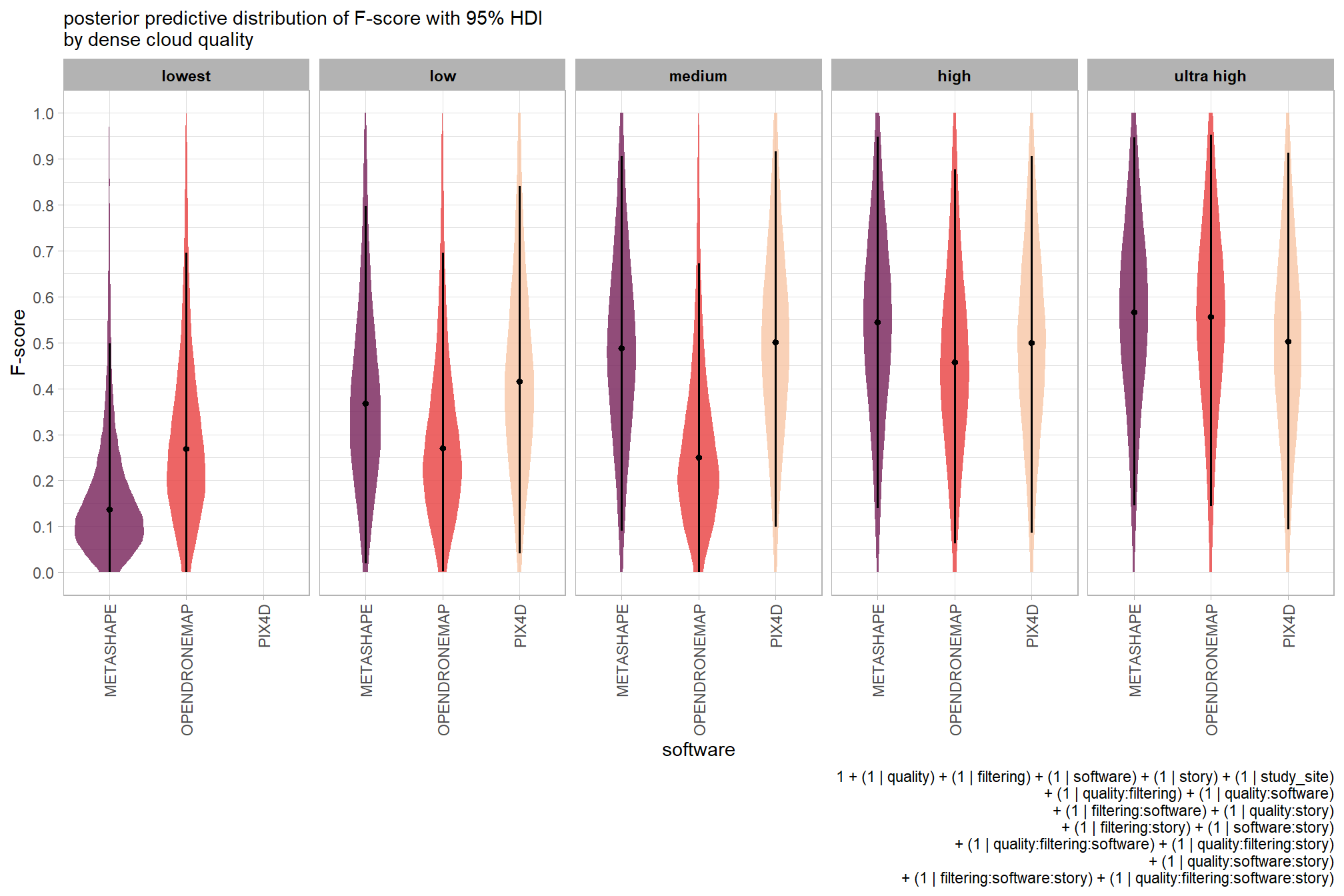
we can also make pairwise comparisons so long as we continue using tidybayes::add_epred_draws with the re_formula argument
# get draws
qlty_sftwr_draws_temp =
tidyr::crossing(
depth_maps_generation_quality = unique(ptcld_validation_data$depth_maps_generation_quality)
, software = unique(ptcld_validation_data$software)
) %>%
tidybayes::add_epred_draws(
brms_f_mod6, allow_new_levels = T
# this part is crucial
, re_formula = ~ (1 | depth_maps_generation_quality) +
(1 | software) +
(1 | depth_maps_generation_quality:software)
) %>%
dplyr::rename(value = .epred)
# calculate contrast
brms_contrast_temp = qlty_sftwr_draws_temp %>%
tidybayes::compare_levels(
value
, by = depth_maps_generation_quality
, comparison = contrast_list
) %>%
dplyr::rename(contrast = depth_maps_generation_quality)
# separate contrast
brms_contrast_temp = brms_contrast_temp %>%
dplyr::ungroup() %>%
tidyr::separate_wider_delim(
cols = contrast
, delim = " - "
, names = paste0(
"sorter"
, 1:(max(stringr::str_count(brms_contrast_temp$contrast, "-"))+1)
)
, too_few = "align_start"
, cols_remove = F
) %>%
dplyr::filter(sorter1!=sorter2) %>%
dplyr::mutate(
dplyr::across(
tidyselect::starts_with("sorter")
, .fns = function(x){factor(
x, ordered = T
, levels = levels(ptcld_validation_data$depth_maps_generation_quality)
)}
)
, contrast = contrast %>%
forcats::fct_reorder(
paste0(as.numeric(sorter1), as.numeric(sorter2)) %>%
as.numeric()
)
) %>%
# median_hdi summary for coloring
dplyr::group_by(contrast, software) %>%
make_contrast_vars()
# remove out-of-sample obs
brms_contrast_temp = brms_contrast_temp %>%
dplyr::inner_join(
ptcld_validation_data %>% dplyr::distinct(software, depth_maps_generation_quality)
, by = dplyr::join_by(software, sorter1 == depth_maps_generation_quality)
) %>%
dplyr::inner_join(
ptcld_validation_data %>% dplyr::distinct(software, depth_maps_generation_quality)
, by = dplyr::join_by(software, sorter2 == depth_maps_generation_quality)
)
# what?
brms_contrast_temp %>% dplyr::glimpse()## Rows: 1,040,000
## Columns: 19
## Groups: contrast, software [26]
## $ software <chr> "METASHAPE", "METASHAPE", "METASHAPE", "METASHAPE", "…
## $ .chain <int> NA, NA, NA, NA, NA, NA, NA, NA, NA, NA, NA, NA, NA, N…
## $ .iteration <int> NA, NA, NA, NA, NA, NA, NA, NA, NA, NA, NA, NA, NA, N…
## $ .draw <int> 1, 2, 3, 4, 5, 6, 7, 8, 9, 10, 11, 12, 13, 14, 15, 16…
## $ sorter1 <ord> ultra high, ultra high, ultra high, ultra high, ultra…
## $ sorter2 <ord> high, high, high, high, high, high, high, high, high,…
## $ contrast <fct> ultra high - high, ultra high - high, ultra high - hi…
## $ value <dbl> 0.158376692, -0.015628733, 0.185569876, 0.151981704, …
## $ median_hdi_est <dbl> 0.01621978, 0.01621978, 0.01621978, 0.01621978, 0.016…
## $ median_hdi_lower <dbl> -0.1248058, -0.1248058, -0.1248058, -0.1248058, -0.12…
## $ median_hdi_upper <dbl> 0.169538, 0.169538, 0.169538, 0.169538, 0.169538, 0.1…
## $ pr_gt_zero <chr> "62%", "62%", "62%", "62%", "62%", "62%", "62%", "62%…
## $ pr_lt_zero <chr> "38%", "38%", "38%", "38%", "38%", "38%", "38%", "38%…
## $ is_diff_dir <lgl> TRUE, FALSE, TRUE, TRUE, FALSE, TRUE, TRUE, TRUE, TRU…
## $ pr_diff <dbl> 0.619, 0.619, 0.619, 0.619, 0.619, 0.619, 0.619, 0.61…
## $ pr_diff_lab <chr> "Pr(ultra high>high)=62%", "Pr(ultra high>high)=62%",…
## $ pr_diff_lab_sm <chr> "Pr(>0)=62%", "Pr(>0)=62%", "Pr(>0)=62%", "Pr(>0)=62%…
## $ pr_diff_lab_pos <dbl> 0.1822533, 0.1822533, 0.1822533, 0.1822533, 0.1822533…
## $ sig_level <ord> <80%, <80%, <80%, <80%, <80%, <80%, <80%, <80%, <80%,…plot it
plt_contrast(
brms_contrast_temp, caption_text = form_temp
, y_axis_title = "quality"
, facet = "software"
, label_size = 2.2
, x_expand = c(0.46,0.75)
) +
labs(
subtitle = "posterior predictive distribution of group constrasts with 95% & 50% HDI\nby software"
)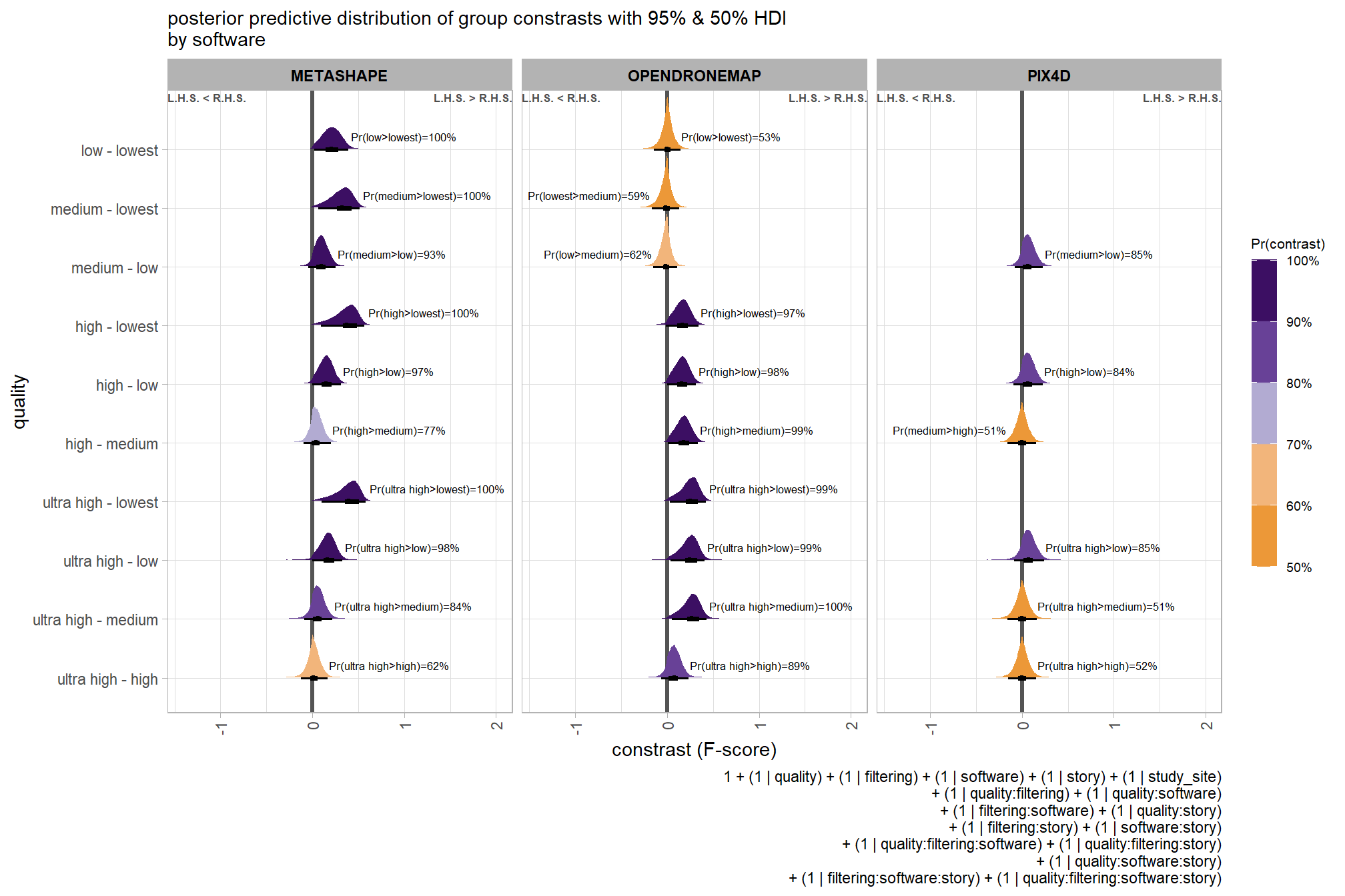
ggplot2::ggsave(
"../data/qlty_sftwr_comp_mod6.png"
, plot = ggplot2::last_plot() + labs(subtitle = "")
, height = 7, width = 10.5
)and summarize these contrasts
brms_contrast_temp %>%
dplyr::group_by(contrast, software, pr_gt_zero) %>%
tidybayes::median_hdi(value) %>%
dplyr::arrange(contrast, software) %>%
dplyr::select(contrast, software, value, .lower, .upper, pr_gt_zero) %>%
dplyr::arrange(software, contrast) %>%
kableExtra::kbl(
digits = 2
, caption = "brms::brm model: 95% HDI of the posterior predictive distribution of group constrasts"
, col.names = c(
"quality contrast"
, "software"
, "difference (F-score)"
, "HDI low", "HDI high"
, "Pr(diff>0)"
)
) %>%
kableExtra::kable_styling() %>%
kableExtra::scroll_box(height = "6in")| quality contrast | software | difference (F-score) | HDI low | HDI high | Pr(diff>0) |
|---|---|---|---|---|---|
| ultra high - high | METASHAPE | 0.02 | -0.12 | 0.17 | 62% |
| ultra high - medium | METASHAPE | 0.06 | -0.08 | 0.22 | 84% |
| ultra high - low | METASHAPE | 0.17 | 0.00 | 0.33 | 98% |
| ultra high - lowest | METASHAPE | 0.40 | 0.10 | 0.58 | 100% |
| high - medium | METASHAPE | 0.04 | -0.10 | 0.20 | 77% |
| high - low | METASHAPE | 0.15 | 0.00 | 0.31 | 97% |
| high - lowest | METASHAPE | 0.38 | 0.09 | 0.57 | 100% |
| medium - low | METASHAPE | 0.10 | -0.04 | 0.25 | 93% |
| medium - lowest | METASHAPE | 0.33 | 0.07 | 0.51 | 100% |
| low - lowest | METASHAPE | 0.21 | 0.02 | 0.39 | 100% |
| ultra high - high | OPENDRONEMAP | 0.08 | -0.06 | 0.23 | 89% |
| ultra high - medium | OPENDRONEMAP | 0.27 | 0.05 | 0.43 | 100% |
| ultra high - low | OPENDRONEMAP | 0.25 | 0.04 | 0.41 | 99% |
| ultra high - lowest | OPENDRONEMAP | 0.25 | 0.03 | 0.42 | 99% |
| high - medium | OPENDRONEMAP | 0.18 | 0.01 | 0.33 | 99% |
| high - low | OPENDRONEMAP | 0.16 | 0.00 | 0.32 | 98% |
| high - lowest | OPENDRONEMAP | 0.17 | -0.01 | 0.34 | 97% |
| medium - low | OPENDRONEMAP | -0.01 | -0.15 | 0.11 | 38% |
| medium - lowest | OPENDRONEMAP | -0.01 | -0.17 | -0.17 | 41% |
| medium - lowest | OPENDRONEMAP | -0.01 | -0.17 | 0.13 | 41% |
| low - lowest | OPENDRONEMAP | 0.00 | -0.14 | 0.15 | 53% |
| ultra high - high | PIX4D | 0.00 | -0.15 | 0.16 | 52% |
| ultra high - medium | PIX4D | 0.00 | -0.16 | 0.16 | 51% |
| ultra high - low | PIX4D | 0.07 | -0.09 | 0.24 | 85% |
| high - medium | PIX4D | 0.00 | -0.16 | 0.15 | 49% |
| high - low | PIX4D | 0.07 | -0.09 | 0.23 | 84% |
| medium - low | PIX4D | 0.07 | -0.08 | 0.23 | 85% |
The contrasts above address the question “are there differences in F-score based on dense point cloud generation quality within each software?”.
To address the different question of “are there differences in F-score based on the processing software used at a given dense point cloud generation quality?” we need to utilize a different formulation of the comparison parameter within our call to the tidybayes::compare_levels function and calculate the contrast by software instead
# calculate contrast
brms_contrast_temp = qlty_sftwr_draws_temp %>%
tidybayes::compare_levels(
value
, by = software
, comparison = "pairwise"
) %>%
dplyr::rename(contrast = software) %>%
# median_hdi summary for coloring
dplyr::group_by(contrast, depth_maps_generation_quality) %>%
make_contrast_vars()
# remove out-of-sample obs
brms_contrast_temp = brms_contrast_temp %>%
tidyr::separate_wider_delim(
cols = contrast
, delim = " - "
, names = paste0(
"sorter"
, 1:(max(stringr::str_count(brms_contrast_temp$contrast, "-"))+1)
)
, too_few = "align_start"
, cols_remove = F
) %>%
dplyr::filter(sorter1!=sorter2) %>%
dplyr::inner_join(
ptcld_validation_data %>% dplyr::distinct(software, depth_maps_generation_quality)
, by = dplyr::join_by(sorter1 == software, depth_maps_generation_quality)
) %>%
dplyr::inner_join(
ptcld_validation_data %>% dplyr::distinct(software, depth_maps_generation_quality)
, by = dplyr::join_by(sorter2 == software, depth_maps_generation_quality)
)
# what?
brms_contrast_temp %>% dplyr::glimpse()## Rows: 520,000
## Columns: 19
## Groups: contrast, depth_maps_generation_quality [13]
## $ depth_maps_generation_quality <ord> ultra high, ultra high, ultra high, ultr…
## $ .chain <int> NA, NA, NA, NA, NA, NA, NA, NA, NA, NA, …
## $ .iteration <int> NA, NA, NA, NA, NA, NA, NA, NA, NA, NA, …
## $ .draw <int> 1, 2, 3, 4, 5, 6, 7, 8, 9, 10, 11, 12, 1…
## $ sorter1 <chr> "OPENDRONEMAP", "OPENDRONEMAP", "OPENDRO…
## $ sorter2 <chr> "METASHAPE", "METASHAPE", "METASHAPE", "…
## $ contrast <chr> "OPENDRONEMAP - METASHAPE", "OPENDRONEMA…
## $ value <dbl> -0.0106825948, -0.0492929373, -0.1107246…
## $ median_hdi_est <dbl> -0.007731576, -0.007731576, -0.007731576…
## $ median_hdi_lower <dbl> -0.2333937, -0.2333937, -0.2333937, -0.2…
## $ median_hdi_upper <dbl> 0.2114123, 0.2114123, 0.2114123, 0.21141…
## $ pr_gt_zero <chr> "46%", "46%", "46%", "46%", "46%", "46%"…
## $ pr_lt_zero <chr> "54%", "54%", "54%", "54%", "54%", "54%"…
## $ is_diff_dir <lgl> TRUE, TRUE, TRUE, TRUE, FALSE, TRUE, FAL…
## $ pr_diff <dbl> 0.54255, 0.54255, 0.54255, 0.54255, 0.54…
## $ pr_diff_lab <chr> "Pr(MtaShp>ODM)=54%", "Pr(MtaShp>ODM)=54…
## $ pr_diff_lab_sm <chr> "Pr(<0)=54%", "Pr(<0)=54%", "Pr(<0)=54%"…
## $ pr_diff_lab_pos <dbl> -0.2508982, -0.2508982, -0.2508982, -0.2…
## $ sig_level <ord> <80%, <80%, <80%, <80%, <80%, <80%, <80%…plot it
plt_contrast(
brms_contrast_temp, caption_text = form_temp
, y_axis_title = "software"
, facet = "depth_maps_generation_quality"
, label_size = 2.0
, x_expand = c(0.17,0.14)
) +
facet_wrap(facets = vars(depth_maps_generation_quality), ncol = 2) +
labs(
subtitle = "posterior predictive distribution of group constrasts with 95% & 50% HDI\nby dense cloud quality"
) +
theme(
legend.position = c(.75, .13)
) +
guides(fill = guide_colorbar(theme = theme(
legend.key.width = unit(1, "lines"),
legend.key.height = unit(7, "lines")
)))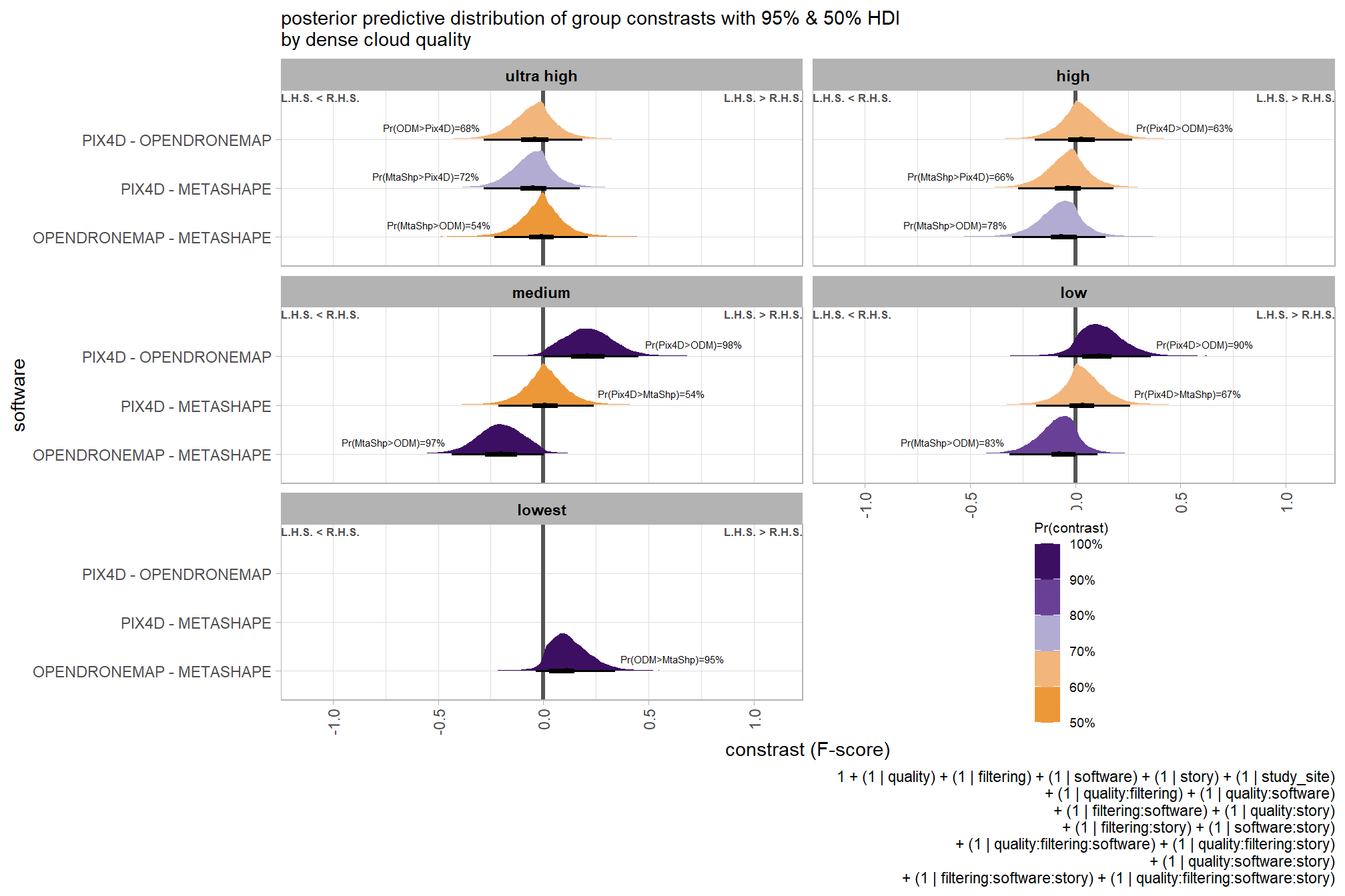
ggplot2::ggsave(
"../data/sftwr_qlty_comp_mod6.png"
, plot = ggplot2::last_plot() + labs(subtitle = "")
, height = 7, width = 10.5
)and summarize these contrasts
brms_contrast_temp %>%
dplyr::group_by(contrast, depth_maps_generation_quality, pr_gt_zero) %>%
tidybayes::median_hdi(value) %>%
dplyr::arrange(contrast, depth_maps_generation_quality) %>%
dplyr::select(contrast, depth_maps_generation_quality, value, .lower, .upper, pr_gt_zero) %>%
kableExtra::kbl(
digits = 2
, caption = "brms::brm model: 95% HDI of the posterior predictive distribution of group constrasts"
, col.names = c(
"software contrast"
, "quality"
, "difference (F-score)"
, "HDI low", "HDI high"
, "Pr(diff>0)"
)
) %>%
kableExtra::kable_styling() %>%
kableExtra::scroll_box(height = "8in")| software contrast | quality | difference (F-score) | HDI low | HDI high | Pr(diff>0) |
|---|---|---|---|---|---|
| OPENDRONEMAP - METASHAPE | ultra high | -0.01 | -0.23 | 0.21 | 46% |
| OPENDRONEMAP - METASHAPE | high | -0.07 | -0.30 | 0.14 | 22% |
| OPENDRONEMAP - METASHAPE | medium | -0.20 | -0.44 | 0.00 | 3% |
| OPENDRONEMAP - METASHAPE | low | -0.08 | -0.31 | 0.11 | 17% |
| OPENDRONEMAP - METASHAPE | lowest | 0.11 | -0.04 | 0.34 | 95% |
| PIX4D - METASHAPE | ultra high | -0.05 | -0.28 | 0.17 | 28% |
| PIX4D - METASHAPE | high | -0.03 | -0.27 | 0.18 | 34% |
| PIX4D - METASHAPE | medium | 0.01 | -0.21 | 0.24 | 54% |
| PIX4D - METASHAPE | low | 0.04 | -0.19 | 0.26 | 67% |
| PIX4D - OPENDRONEMAP | ultra high | -0.04 | -0.28 | 0.19 | 32% |
| PIX4D - OPENDRONEMAP | high | 0.03 | -0.19 | 0.27 | 63% |
| PIX4D - OPENDRONEMAP | medium | 0.21 | 0.00 | 0.45 | 98% |
| PIX4D - OPENDRONEMAP | low | 0.12 | -0.08 | 0.36 | 90% |
6.9.2.6 Software:Filtering - interaction
Are there differences in F-score based on dense point cloud filtering mode within each processing software?
Here, we collapse across the study site, depth map generation quality, and story to compare the combined filtering mode and software effect.
In a hierarchical model structure, we have to make use of the re_formula argument within tidybayes::add_epred_draws
Even though filtering mode had a small effect on the SfM predictive ability when averaging across all softwares, there might still be differences in filtering mode within software when we average across all depth map generation quality settings. Let’s check the difference in F-score by depth map filtering mode and software.
# get draws
fltr_sftwr_draws_temp = ptcld_validation_data %>%
dplyr::distinct(depth_maps_generation_filtering_mode, software) %>%
tidybayes::add_epred_draws(
brms_f_mod6, allow_new_levels = T
# this part is crucial
, re_formula = ~ (1 | depth_maps_generation_filtering_mode) +
(1 | software) +
(1 | depth_maps_generation_filtering_mode:software)
) %>%
dplyr::rename(value = .epred)
# plot
fltr_sftwr_draws_temp %>%
ggplot(
mapping = aes(
y = value, x = software
, fill = software
)
) +
tidybayes::stat_eye(
point_interval = median_hdi, .width = .95
, slab_alpha = 0.8
, interval_color = "black", linewidth = 1
, point_color = "black", point_fill = "black", point_size = 1
) +
scale_fill_viridis_d(option = "rocket", begin = 0.3, end = 0.9, drop = F) +
scale_y_continuous(breaks = scales::extended_breaks(n=10)) +
facet_grid(cols = vars(depth_maps_generation_filtering_mode)) +
labs(
x = "software", y = "F-score"
, subtitle = "posterior predictive distribution of F-score with 95% HDI\nby filtering mode"
, caption = form_temp
) +
theme_light() +
theme(
legend.position = "none"
, legend.direction = "horizontal"
, axis.text.x = element_text(angle = 90, vjust = 0.5, hjust = 1)
, strip.text = element_text(color = "black", face = "bold")
) 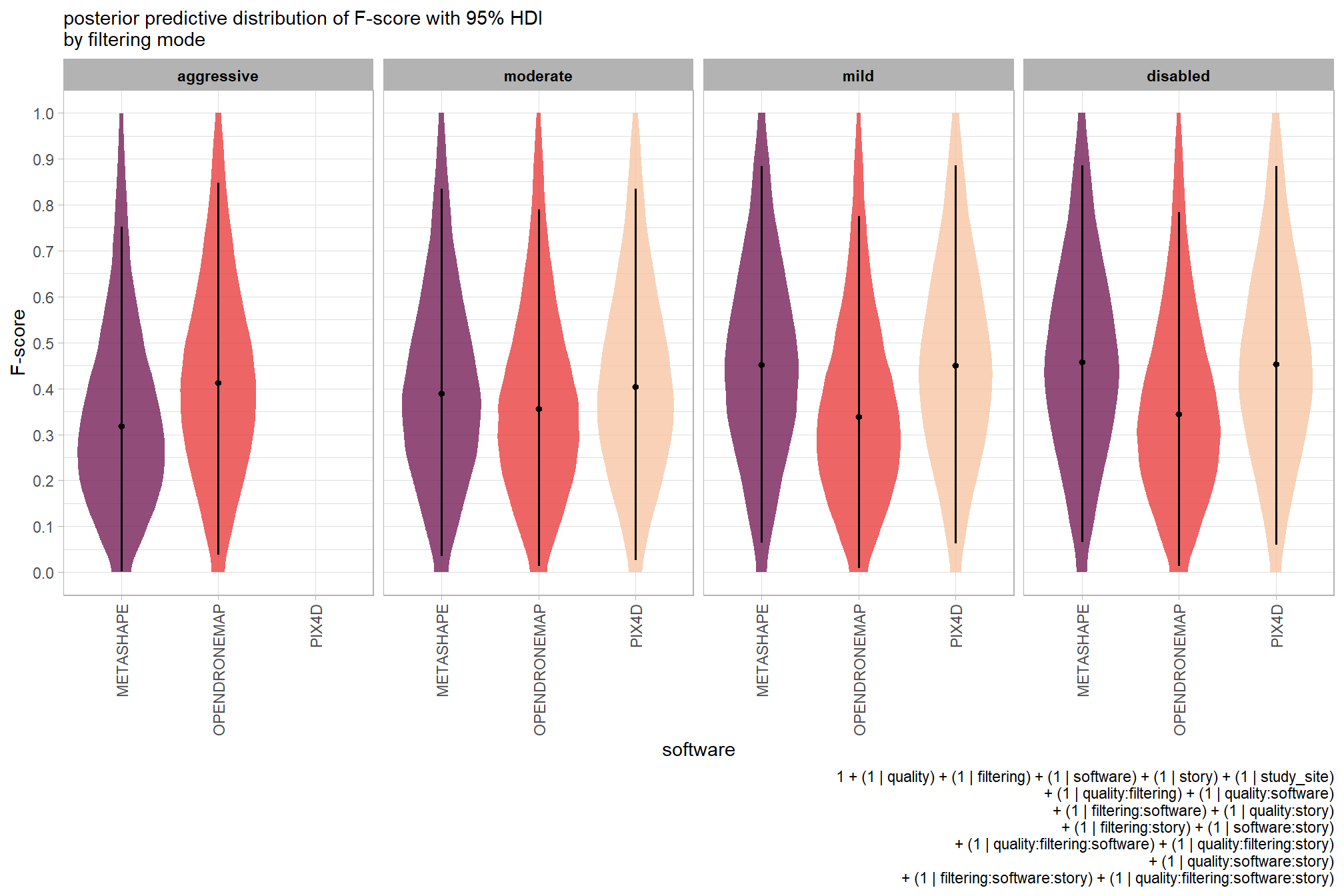
we can also make pairwise comparisons so long as we continue using tidybayes::add_epred_draws with the re_formula argument
# calculate contrast
brms_contrast_temp = fltr_sftwr_draws_temp %>%
tidybayes::compare_levels(
value
, by = depth_maps_generation_filtering_mode
, comparison = "pairwise"
) %>%
dplyr::rename(contrast = depth_maps_generation_filtering_mode)
# separate contrast
brms_contrast_temp = brms_contrast_temp %>%
dplyr::ungroup() %>%
tidyr::separate_wider_delim(
cols = contrast
, delim = " - "
, names = paste0(
"sorter"
, 1:(max(stringr::str_count(brms_contrast_temp$contrast, "-"))+1)
)
, too_few = "align_start"
, cols_remove = F
) %>%
dplyr::filter(sorter1!=sorter2) %>%
dplyr::mutate(
dplyr::across(
tidyselect::starts_with("sorter")
, .fns = function(x){factor(
x, ordered = T
, levels = levels(ptcld_validation_data$depth_maps_generation_filtering_mode)
)}
)
, contrast = contrast %>%
forcats::fct_reorder(
paste0(as.numeric(sorter1), as.numeric(sorter2)) %>%
as.numeric()
) %>%
# re order for filtering mode
forcats::fct_rev()
) %>%
# median_hdi summary for coloring
dplyr::group_by(contrast, software) %>%
make_contrast_vars()
# what?
brms_contrast_temp %>% dplyr::glimpse()## Rows: 600,000
## Columns: 19
## Groups: contrast, software [15]
## $ software <chr> "METASHAPE", "METASHAPE", "METASHAPE", "METASHAPE", "…
## $ .chain <int> NA, NA, NA, NA, NA, NA, NA, NA, NA, NA, NA, NA, NA, N…
## $ .iteration <int> NA, NA, NA, NA, NA, NA, NA, NA, NA, NA, NA, NA, NA, N…
## $ .draw <int> 1, 2, 3, 4, 5, 6, 7, 8, 9, 10, 11, 12, 13, 14, 15, 16…
## $ sorter1 <ord> moderate, moderate, moderate, moderate, moderate, mod…
## $ sorter2 <ord> aggressive, aggressive, aggressive, aggressive, aggre…
## $ contrast <fct> moderate - aggressive, moderate - aggressive, moderat…
## $ value <dbl> -0.006856818, 0.076603376, 0.060906550, 0.053213815, …
## $ median_hdi_est <dbl> 0.05709402, 0.05709402, 0.05709402, 0.05709402, 0.057…
## $ median_hdi_lower <dbl> -0.02673803, -0.02673803, -0.02673803, -0.02673803, -…
## $ median_hdi_upper <dbl> 0.1642191, 0.1642191, 0.1642191, 0.1642191, 0.1642191…
## $ pr_gt_zero <chr> "92%", "92%", "92%", "92%", "92%", "92%", "92%", "92%…
## $ pr_lt_zero <chr> "8%", "8%", "8%", "8%", "8%", "8%", "8%", "8%", "8%",…
## $ is_diff_dir <lgl> FALSE, TRUE, TRUE, TRUE, TRUE, TRUE, TRUE, TRUE, TRUE…
## $ pr_diff <dbl> 0.9202, 0.9202, 0.9202, 0.9202, 0.9202, 0.9202, 0.920…
## $ pr_diff_lab <chr> "Pr(moderate>aggressive)=92%", "Pr(moderate>aggressiv…
## $ pr_diff_lab_sm <chr> "Pr(>0)=92%", "Pr(>0)=92%", "Pr(>0)=92%", "Pr(>0)=92%…
## $ pr_diff_lab_pos <dbl> 0.1765355, 0.1765355, 0.1765355, 0.1765355, 0.1765355…
## $ sig_level <ord> 90%, 90%, 90%, 90%, 90%, 90%, 90%, 90%, 90%, 90%, 90%…plot it
plt_contrast(
brms_contrast_temp, caption_text = form_temp
, y_axis_title = "filtering mode"
, facet = "software"
, label_size = 2.0
, x_expand = c(0.85,0.8) # c(1,1.4)
) +
labs(
subtitle = "posterior predictive distribution of group constrasts with 95% & 50% HDI\nby software"
)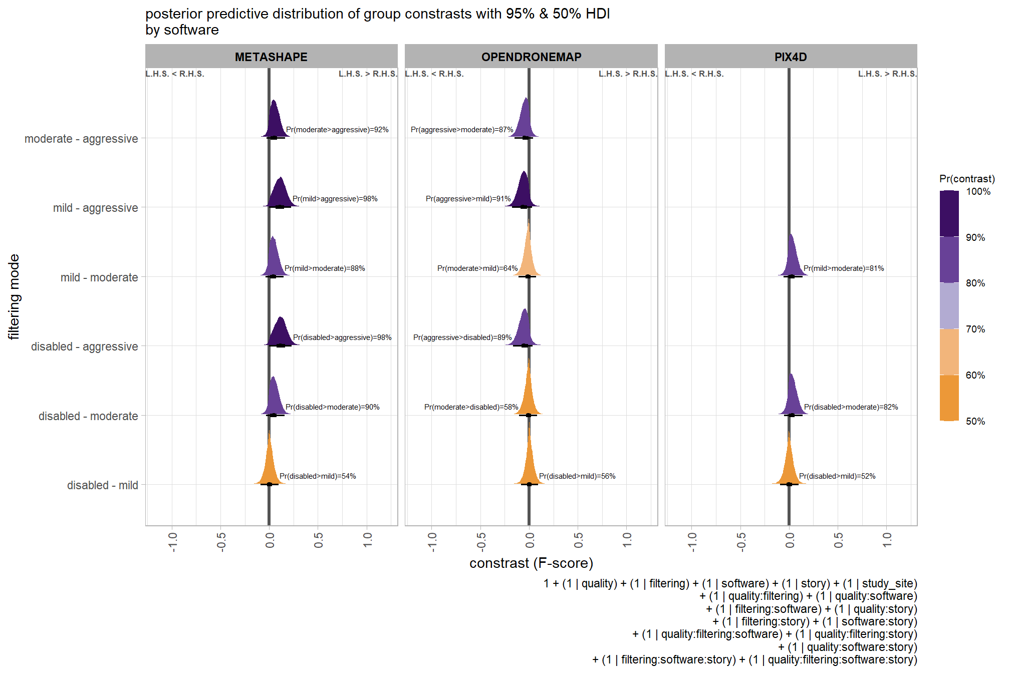
ggplot2::ggsave(
"../data/fltr_sftwr_comp_mod6.png"
, plot = ggplot2::last_plot() + labs(subtitle = "")
, height = 7, width = 10.5
)and summarize these contrasts
brms_contrast_temp %>%
dplyr::group_by(contrast, software, pr_gt_zero) %>%
tidybayes::median_hdi(value) %>%
dplyr::arrange(contrast, software) %>%
dplyr::select(contrast, software, value, .lower, .upper, pr_gt_zero) %>%
dplyr::arrange(software, contrast) %>%
kableExtra::kbl(
digits = 2
, caption = "brms::brm model: 95% HDI of the posterior predictive distribution of group constrasts"
, col.names = c(
"filtering contrast"
, "software"
, "difference (F-score)"
, "HDI low", "HDI high"
, "Pr(diff>0)"
)
) %>%
kableExtra::kable_styling() %>%
kableExtra::scroll_box(height = "6in")| filtering contrast | software | difference (F-score) | HDI low | HDI high | Pr(diff>0) |
|---|---|---|---|---|---|
| disabled - mild | METASHAPE | 0.00 | -0.09 | 0.10 | 54% |
| disabled - moderate | METASHAPE | 0.05 | -0.03 | 0.16 | 90% |
| disabled - aggressive | METASHAPE | 0.12 | 0.00 | 0.23 | 98% |
| mild - moderate | METASHAPE | 0.05 | -0.04 | 0.15 | 88% |
| mild - aggressive | METASHAPE | 0.11 | 0.00 | 0.22 | 98% |
| moderate - aggressive | METASHAPE | 0.06 | -0.03 | 0.16 | 92% |
| disabled - mild | OPENDRONEMAP | 0.00 | -0.08 | 0.09 | 56% |
| disabled - moderate | OPENDRONEMAP | -0.01 | -0.10 | 0.08 | 42% |
| disabled - aggressive | OPENDRONEMAP | -0.05 | -0.16 | 0.04 | 11% |
| mild - moderate | OPENDRONEMAP | -0.01 | -0.11 | 0.07 | 36% |
| mild - aggressive | OPENDRONEMAP | -0.06 | -0.17 | 0.03 | 9% |
| moderate - aggressive | OPENDRONEMAP | -0.04 | -0.15 | 0.04 | 13% |
| disabled - mild | PIX4D | 0.00 | -0.09 | 0.10 | 52% |
| disabled - moderate | PIX4D | 0.04 | -0.05 | 0.14 | 82% |
| mild - moderate | PIX4D | 0.03 | -0.05 | 0.14 | 81% |
6.9.2.7 Software:Quality:Filtering - interaction
The contrasts immediately above address the question “are there differences in F-score based on dense point cloud filtering mode within each software?”. Although the impact of filtering mode is small, it is highly probable when averaging across all quality settings. What if we don’t average out the impact of quality and instead get the full, three-way interaction between software, quality, and filtering mode?
Let’s get the model’s answer to the question “For each software, are there differences in F-score based on dense point cloud filtering mode within each point cloud generation quality?”.
Here, we collapse across the study site and story to compare the dense cloud quality, filtering mode, and software effect.
In a hierarchical model structure, we have to make use of the re_formula argument within tidybayes::add_epred_draws
# get draws
fltr_sftwr_draws_temp =
tidyr::crossing(
depth_maps_generation_quality = unique(ptcld_validation_data$depth_maps_generation_quality)
, depth_maps_generation_filtering_mode = unique(ptcld_validation_data$depth_maps_generation_filtering_mode)
, software = unique(ptcld_validation_data$software)
) %>%
tidybayes::add_epred_draws(
brms_f_mod6, allow_new_levels = T
# this part is crucial
, re_formula = ~ (1 | depth_maps_generation_quality) + # main effects
(1 | depth_maps_generation_quality) +
(1 | depth_maps_generation_filtering_mode) +
(1 | software) +
# two-way interactions
(1 | depth_maps_generation_quality:depth_maps_generation_filtering_mode) +
(1 | depth_maps_generation_quality:software) +
(1 | depth_maps_generation_filtering_mode:software) +
# three-way interactions
(1 | depth_maps_generation_quality:depth_maps_generation_filtering_mode:software)
) %>%
dplyr::rename(value = .epred)
# plot
fltr_sftwr_draws_temp %>%
dplyr::inner_join(
ptcld_validation_data %>% dplyr::distinct(software, depth_maps_generation_quality, depth_maps_generation_filtering_mode)
, by = dplyr::join_by(software, depth_maps_generation_quality, depth_maps_generation_filtering_mode)
) %>%
dplyr::mutate(depth_maps_generation_quality = depth_maps_generation_quality %>% forcats::fct_rev()) %>%
ggplot(
mapping = aes(
y = value
, x = depth_maps_generation_filtering_mode
, fill = depth_maps_generation_filtering_mode
)
) +
tidybayes::stat_eye(
point_interval = median_hdi, .width = .95
, slab_alpha = 0.8
, interval_color = "black", linewidth = 1
, point_color = "black", point_fill = "black", point_size = 1
) +
scale_fill_viridis_d(option = "plasma", drop = F) +
scale_y_continuous(breaks = scales::extended_breaks(n=10)) +
facet_grid(
rows = vars(software)
, cols = vars(depth_maps_generation_quality)
# , switch = "y"
) +
labs(
fill = "filtering mode"
, x = "filtering mode", y = "F-score"
, subtitle = "posterior predictive distribution of F-score with 95% HDI\nby dense cloud quality and software"
# , caption = form_temp
) +
theme_light() +
theme(
legend.position = "top"
, legend.direction = "horizontal"
, axis.text.x = element_text(angle = 90, vjust = 0.5, hjust = 1)
, strip.text = element_text(color = "black", face = "bold")
# , strip.placement = "outside"
) +
guides(
fill = guide_legend(override.aes = list(shape = NA, size = 6, alpha = 0.9, lwd = NA))
)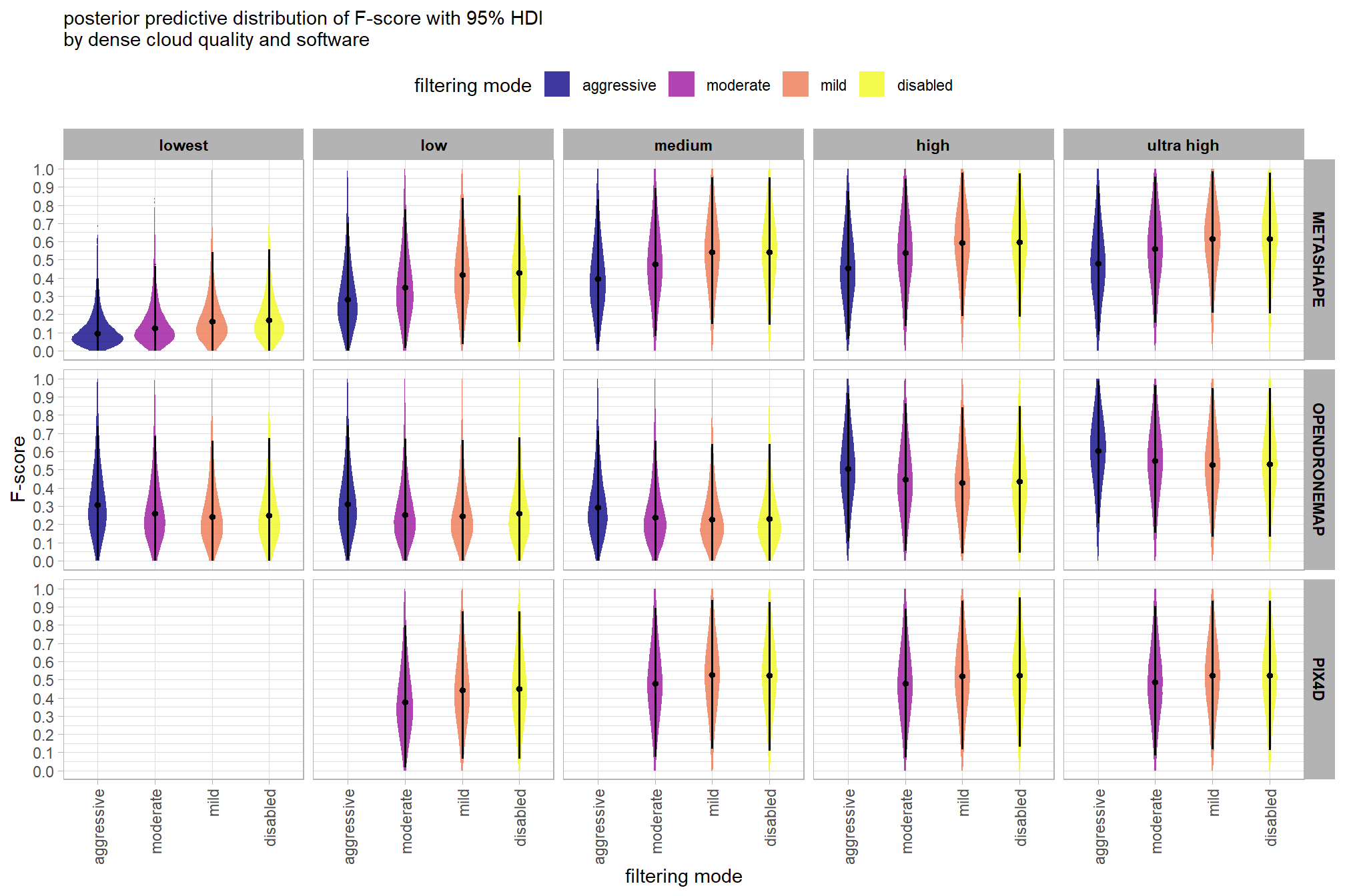
ggplot2::ggsave(
"../data/qlty_fltr_sftwr_mod6.png"
, plot = ggplot2::last_plot() + labs(subtitle = "")
, height = 7, width = 10.5
)we can also make pairwise comparisons so long as we continue using tidybayes::add_epred_draws with the re_formula argument
# calculate contrast
brms_contrast_temp = fltr_sftwr_draws_temp %>%
tidybayes::compare_levels(
value
, by = depth_maps_generation_filtering_mode
, comparison = "pairwise"
) %>%
dplyr::rename(contrast = depth_maps_generation_filtering_mode)
# separate contrast
brms_contrast_temp = brms_contrast_temp %>%
dplyr::ungroup() %>%
tidyr::separate_wider_delim(
cols = contrast
, delim = " - "
, names = paste0(
"sorter"
, 1:(max(stringr::str_count(brms_contrast_temp$contrast, "-"))+1)
)
, too_few = "align_start"
, cols_remove = F
) %>%
dplyr::filter(sorter1!=sorter2) %>%
dplyr::mutate(
dplyr::across(
tidyselect::starts_with("sorter")
, .fns = function(x){factor(
x, ordered = T
, levels = levels(ptcld_validation_data$depth_maps_generation_filtering_mode)
)}
)
, contrast = contrast %>%
forcats::fct_reorder(
paste0(as.numeric(sorter1), as.numeric(sorter2)) %>%
as.numeric()
) %>%
# re order for filtering mode
forcats::fct_rev()
) %>%
# median_hdi summary for coloring
dplyr::group_by(contrast, software, depth_maps_generation_quality) %>%
make_contrast_vars()
# remove out-of-sample obs
brms_contrast_temp = brms_contrast_temp %>%
dplyr::inner_join(
ptcld_validation_data %>% dplyr::distinct(software, depth_maps_generation_quality, depth_maps_generation_filtering_mode)
, by = dplyr::join_by(software, depth_maps_generation_quality, sorter1==depth_maps_generation_filtering_mode)
) %>%
dplyr::inner_join(
ptcld_validation_data %>% dplyr::distinct(software, depth_maps_generation_quality, depth_maps_generation_filtering_mode)
, by = dplyr::join_by(software, depth_maps_generation_quality, sorter2==depth_maps_generation_filtering_mode)
) %>%
dplyr::mutate(depth_maps_generation_quality = depth_maps_generation_quality %>% forcats::fct_rev())
# what?
brms_contrast_temp %>% dplyr::glimpse()## Rows: 2,880,000
## Columns: 20
## Groups: contrast, software, depth_maps_generation_quality [72]
## $ depth_maps_generation_quality <ord> ultra high, ultra high, ultra high, ultr…
## $ software <chr> "METASHAPE", "METASHAPE", "METASHAPE", "…
## $ .chain <int> NA, NA, NA, NA, NA, NA, NA, NA, NA, NA, …
## $ .iteration <int> NA, NA, NA, NA, NA, NA, NA, NA, NA, NA, …
## $ .draw <int> 1, 2, 3, 4, 5, 6, 7, 8, 9, 10, 11, 12, 1…
## $ sorter1 <ord> moderate, moderate, moderate, moderate, …
## $ sorter2 <ord> aggressive, aggressive, aggressive, aggr…
## $ contrast <fct> moderate - aggressive, moderate - aggres…
## $ value <dbl> -0.003468489, 0.068129488, 0.092618344, …
## $ median_hdi_est <dbl> 0.06468366, 0.06468366, 0.06468366, 0.06…
## $ median_hdi_lower <dbl> -0.03619306, -0.03619306, -0.03619306, -…
## $ median_hdi_upper <dbl> 0.1828082, 0.1828082, 0.1828082, 0.18280…
## $ pr_gt_zero <chr> "91%", "91%", "91%", "91%", "91%", "91%"…
## $ pr_lt_zero <chr> "9%", "9%", "9%", "9%", "9%", "9%", "9%"…
## $ is_diff_dir <lgl> FALSE, TRUE, TRUE, TRUE, TRUE, TRUE, TRU…
## $ pr_diff <dbl> 0.90815, 0.90815, 0.90815, 0.90815, 0.90…
## $ pr_diff_lab <chr> "Pr(moderate>aggressive)=91%", "Pr(moder…
## $ pr_diff_lab_sm <chr> "Pr(>0)=91%", "Pr(>0)=91%", "Pr(>0)=91%"…
## $ pr_diff_lab_pos <dbl> 0.1965188, 0.1965188, 0.1965188, 0.19651…
## $ sig_level <ord> 90%, 90%, 90%, 90%, 90%, 90%, 90%, 90%, …plot it
brms_contrast_temp %>%
plt_contrast(
facet = c("depth_maps_generation_quality", "software")
, y_axis_title = "filtering mode"
, label_size = 0
, x_expand = c(-0.1,-0.1)
) +
facet_grid(
rows = vars(software)
, cols = vars(depth_maps_generation_quality)
) +
labs(
subtitle = "posterior predictive distribution of group constrasts with 95% & 50% HDI\nby dense cloud quality and software"
)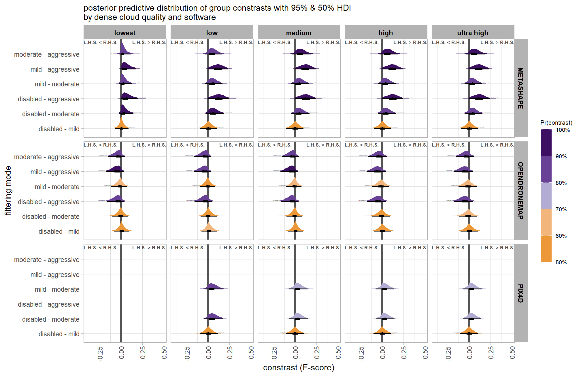
6.9.2.8 Quality - main effect
let’s collapse across the story, filtering mode, software, and study site to compare the dense cloud quality setting effect.
In a hierarchical model structure, we have to make use of the re_formula argument within tidybayes::add_epred_draws
ptcld_validation_data %>%
dplyr::distinct(depth_maps_generation_quality) %>%
tidybayes::add_epred_draws(
brms_f_mod6
# this part is crucial
, re_formula = ~ (1 | depth_maps_generation_quality)
) %>%
dplyr::rename(value = .epred) %>%
# plot
ggplot(
mapping = aes(
x = value, y = depth_maps_generation_quality
, fill = depth_maps_generation_quality
)
) +
tidybayes::stat_halfeye(
point_interval = median_hdi, .width = .95
, interval_color = "gray66"
, shape = 21, point_color = "gray66", point_fill = "black"
, justification = -0.01
) +
scale_fill_viridis_d(option = "inferno", drop = F) +
scale_x_continuous(breaks = scales::extended_breaks(n=8)) +
labs(
y = "quality", x = "F-score"
, subtitle = "posterior predictive distribution of F-score with 95% HDI"
, caption = form_temp
) +
theme_light() +
theme(legend.position = "none")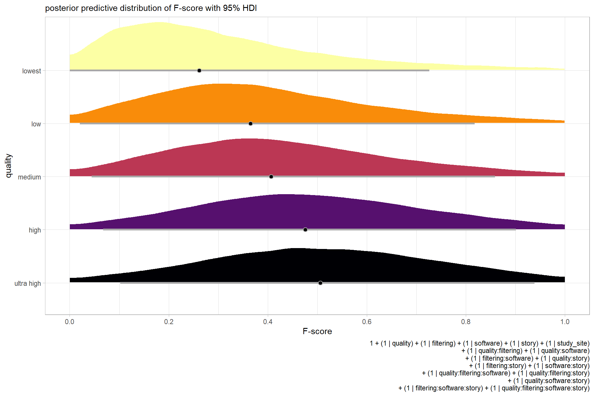
we can also perform pairwise comparisons
brms_contrast_temp =
ptcld_validation_data %>%
dplyr::distinct(depth_maps_generation_quality) %>%
tidybayes::add_epred_draws(
brms_f_mod6, allow_new_levels = T
# this part is crucial
, re_formula = ~ (1 | depth_maps_generation_quality)
) %>%
dplyr::rename(value = .epred) %>%
tidybayes::compare_levels(
value
, by = depth_maps_generation_quality
, comparison =
contrast_list
# tidybayes::emmeans_comparison("revpairwise")
#"pairwise"
) %>%
dplyr::rename(contrast = depth_maps_generation_quality)
# separate contrast
brms_contrast_temp = brms_contrast_temp %>%
dplyr::ungroup() %>%
tidyr::separate_wider_delim(
cols = contrast
, delim = " - "
, names = paste0(
"sorter"
, 1:(max(stringr::str_count(brms_contrast_temp$contrast, "-"))+1)
)
, too_few = "align_start"
, cols_remove = F
) %>%
dplyr::filter(sorter1!=sorter2) %>%
dplyr::mutate(
dplyr::across(
tidyselect::starts_with("sorter")
, .fns = function(x){factor(
x, ordered = T
, levels = levels(ptcld_validation_data$depth_maps_generation_quality)
)}
)
, contrast = contrast %>%
forcats::fct_reorder(
paste0(as.numeric(sorter1), as.numeric(sorter2)) %>%
as.numeric()
)
) %>%
# median_hdi summary for coloring
dplyr::group_by(contrast) %>%
make_contrast_vars()
# what?
brms_contrast_temp %>% dplyr::glimpse()## Rows: 400,000
## Columns: 18
## Groups: contrast [10]
## $ .chain <int> NA, NA, NA, NA, NA, NA, NA, NA, NA, NA, NA, NA, NA, N…
## $ .iteration <int> NA, NA, NA, NA, NA, NA, NA, NA, NA, NA, NA, NA, NA, N…
## $ .draw <int> 1, 2, 3, 4, 5, 6, 7, 8, 9, 10, 11, 12, 13, 14, 15, 16…
## $ sorter1 <ord> ultra high, ultra high, ultra high, ultra high, ultra…
## $ sorter2 <ord> high, high, high, high, high, high, high, high, high,…
## $ contrast <fct> ultra high - high, ultra high - high, ultra high - hi…
## $ value <dbl> 0.081821389, 0.010165042, -0.004214973, -0.006332847,…
## $ median_hdi_est <dbl> 0.01748438, 0.01748438, 0.01748438, 0.01748438, 0.017…
## $ median_hdi_lower <dbl> -0.1672428, -0.1672428, -0.1672428, -0.1672428, -0.16…
## $ median_hdi_upper <dbl> 0.2111465, 0.2111465, 0.2111465, 0.2111465, 0.2111465…
## $ pr_gt_zero <chr> "62%", "62%", "62%", "62%", "62%", "62%", "62%", "62%…
## $ pr_lt_zero <chr> "38%", "38%", "38%", "38%", "38%", "38%", "38%", "38%…
## $ is_diff_dir <lgl> TRUE, TRUE, FALSE, FALSE, FALSE, TRUE, FALSE, FALSE, …
## $ pr_diff <dbl> 0.61515, 0.61515, 0.61515, 0.61515, 0.61515, 0.61515,…
## $ pr_diff_lab <chr> "Pr(ultra high>high)=62%", "Pr(ultra high>high)=62%",…
## $ pr_diff_lab_sm <chr> "Pr(>0)=62%", "Pr(>0)=62%", "Pr(>0)=62%", "Pr(>0)=62%…
## $ pr_diff_lab_pos <dbl> 0.2269825, 0.2269825, 0.2269825, 0.2269825, 0.2269825…
## $ sig_level <ord> <80%, <80%, <80%, <80%, <80%, <80%, <80%, <80%, <80%,…plot it
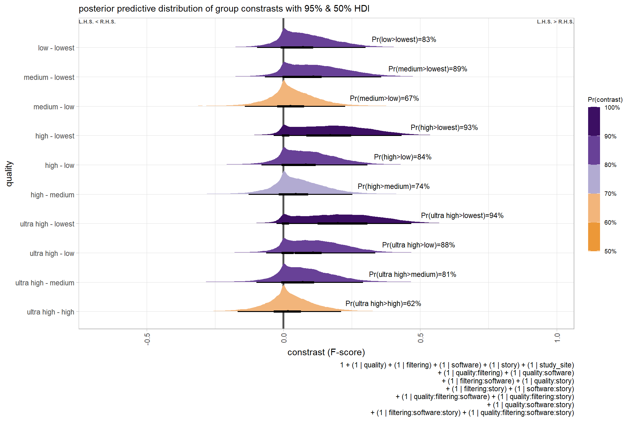
and summarize these contrasts
brms_contrast_temp %>%
dplyr::group_by(contrast, pr_gt_zero) %>%
tidybayes::median_hdi(value) %>%
dplyr::arrange(contrast) %>%
dplyr::select(contrast, value, .lower, .upper, pr_gt_zero) %>%
kableExtra::kbl(
digits = 2
, caption = "brms::brm model: 95% HDI of the posterior predictive distribution of group constrasts"
, col.names = c(
"quality contrast"
, "difference (F-score)"
, "HDI low", "HDI high"
, "Pr(diff>0)"
)
) %>%
kableExtra::kable_styling()| quality contrast | difference (F-score) | HDI low | HDI high | Pr(diff>0) |
|---|---|---|---|---|
| ultra high - high | 0.02 | -0.17 | 0.21 | 62% |
| ultra high - medium | 0.07 | -0.10 | 0.29 | 81% |
| ultra high - low | 0.11 | -0.06 | 0.34 | 88% |
| ultra high - lowest | 0.20 | -0.03 | 0.47 | 94% |
| high - medium | 0.05 | -0.13 | 0.25 | 74% |
| high - low | 0.08 | -0.08 | 0.31 | 84% |
| high - lowest | 0.17 | -0.04 | 0.43 | 93% |
| medium - low | 0.03 | -0.14 | 0.23 | 67% |
| medium - lowest | 0.11 | -0.07 | 0.36 | 89% |
| low - lowest | 0.07 | -0.10 | 0.30 | 83% |
6.9.2.9 Filtering - main effect
let’s collapse across the story, dense cloud quality, software, and study site to compare the filtering mode setting effect.
In a hierarchical model structure, we have to make use of the re_formula argument within tidybayes::add_epred_draws
ptcld_validation_data %>%
dplyr::distinct(depth_maps_generation_filtering_mode) %>%
tidybayes::add_epred_draws(
brms_f_mod6
# this part is crucial
, re_formula = ~ (1 | depth_maps_generation_filtering_mode)
) %>%
dplyr::rename(value = .epred) %>%
# plot
ggplot(
mapping = aes(
x = value, y = depth_maps_generation_filtering_mode
, fill = depth_maps_generation_filtering_mode
)
) +
tidybayes::stat_halfeye(
point_interval = median_hdi, .width = .95
, interval_color = "gray66"
, shape = 21, point_color = "gray66", point_fill = "black"
, justification = -0.01
) +
scale_fill_viridis_d(option = "plasma", drop = F) +
scale_x_continuous(breaks = scales::extended_breaks(n=8)) +
labs(
y = "filtering mode", x = "F-score"
, subtitle = "posterior predictive distribution of F-score with 95% HDI"
, caption = form_temp
) +
theme_light() +
theme(legend.position = "none")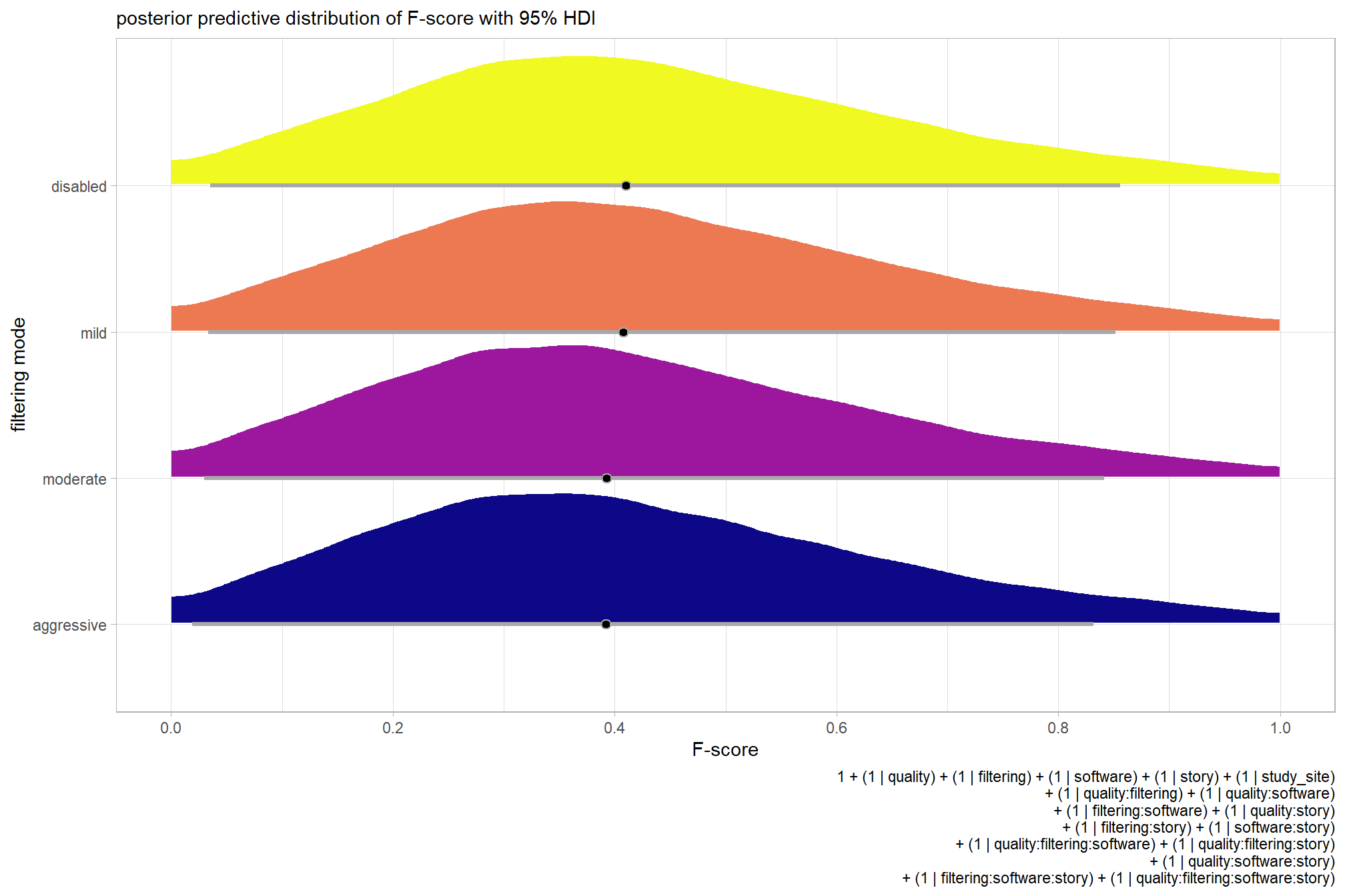
we can also perform pairwise comparisons
brms_contrast_temp =
ptcld_validation_data %>%
dplyr::distinct(depth_maps_generation_filtering_mode) %>%
tidybayes::add_epred_draws(
brms_f_mod6, allow_new_levels = T
# this part is crucial
, re_formula = ~ (1 | depth_maps_generation_filtering_mode)
) %>%
dplyr::rename(value = .epred) %>%
tidybayes::compare_levels(
value
, by = depth_maps_generation_filtering_mode
, comparison = "pairwise"
) %>%
dplyr::rename(contrast = depth_maps_generation_filtering_mode)
# separate contrast
brms_contrast_temp = brms_contrast_temp %>%
dplyr::ungroup() %>%
tidyr::separate_wider_delim(
cols = contrast
, delim = " - "
, names = paste0(
"sorter"
, 1:(max(stringr::str_count(brms_contrast_temp$contrast, "-"))+1)
)
, too_few = "align_start"
, cols_remove = F
) %>%
dplyr::filter(sorter1!=sorter2) %>%
dplyr::mutate(
dplyr::across(
tidyselect::starts_with("sorter")
, .fns = function(x){factor(
x, ordered = T
, levels = levels(ptcld_validation_data$depth_maps_generation_filtering_mode)
)}
)
, contrast = contrast %>%
forcats::fct_reorder(
paste0(as.numeric(sorter1), as.numeric(sorter2)) %>%
as.numeric()
) %>%
# re order for filtering mode
forcats::fct_rev()
) %>%
# median_hdi summary for coloring
dplyr::group_by(contrast) %>%
make_contrast_vars()
# what?
brms_contrast_temp %>% dplyr::glimpse()## Rows: 240,000
## Columns: 18
## Groups: contrast [6]
## $ .chain <int> NA, NA, NA, NA, NA, NA, NA, NA, NA, NA, NA, NA, NA, N…
## $ .iteration <int> NA, NA, NA, NA, NA, NA, NA, NA, NA, NA, NA, NA, NA, N…
## $ .draw <int> 1, 2, 3, 4, 5, 6, 7, 8, 9, 10, 11, 12, 13, 14, 15, 16…
## $ sorter1 <ord> moderate, moderate, moderate, moderate, moderate, mod…
## $ sorter2 <ord> aggressive, aggressive, aggressive, aggressive, aggre…
## $ contrast <fct> moderate - aggressive, moderate - aggressive, moderat…
## $ value <dbl> -0.0103292621, -0.0367862977, -0.0056778029, -0.00166…
## $ median_hdi_est <dbl> 0.0001174049, 0.0001174049, 0.0001174049, 0.000117404…
## $ median_hdi_lower <dbl> -0.09076018, -0.09076018, -0.09076018, -0.09076018, -…
## $ median_hdi_upper <dbl> 0.09457266, 0.09457266, 0.09457266, 0.09457266, 0.094…
## $ pr_gt_zero <chr> "51%", "51%", "51%", "51%", "51%", "51%", "51%", "51%…
## $ pr_lt_zero <chr> "49%", "49%", "49%", "49%", "49%", "49%", "49%", "49%…
## $ is_diff_dir <lgl> FALSE, FALSE, FALSE, FALSE, FALSE, FALSE, TRUE, TRUE,…
## $ pr_diff <dbl> 0.507075, 0.507075, 0.507075, 0.507075, 0.507075, 0.5…
## $ pr_diff_lab <chr> "Pr(moderate>aggressive)=51%", "Pr(moderate>aggressiv…
## $ pr_diff_lab_sm <chr> "Pr(>0)=51%", "Pr(>0)=51%", "Pr(>0)=51%", "Pr(>0)=51%…
## $ pr_diff_lab_pos <dbl> 0.1016656, 0.1016656, 0.1016656, 0.1016656, 0.1016656…
## $ sig_level <ord> <80%, <80%, <80%, <80%, <80%, <80%, <80%, <80%, <80%,…plot it
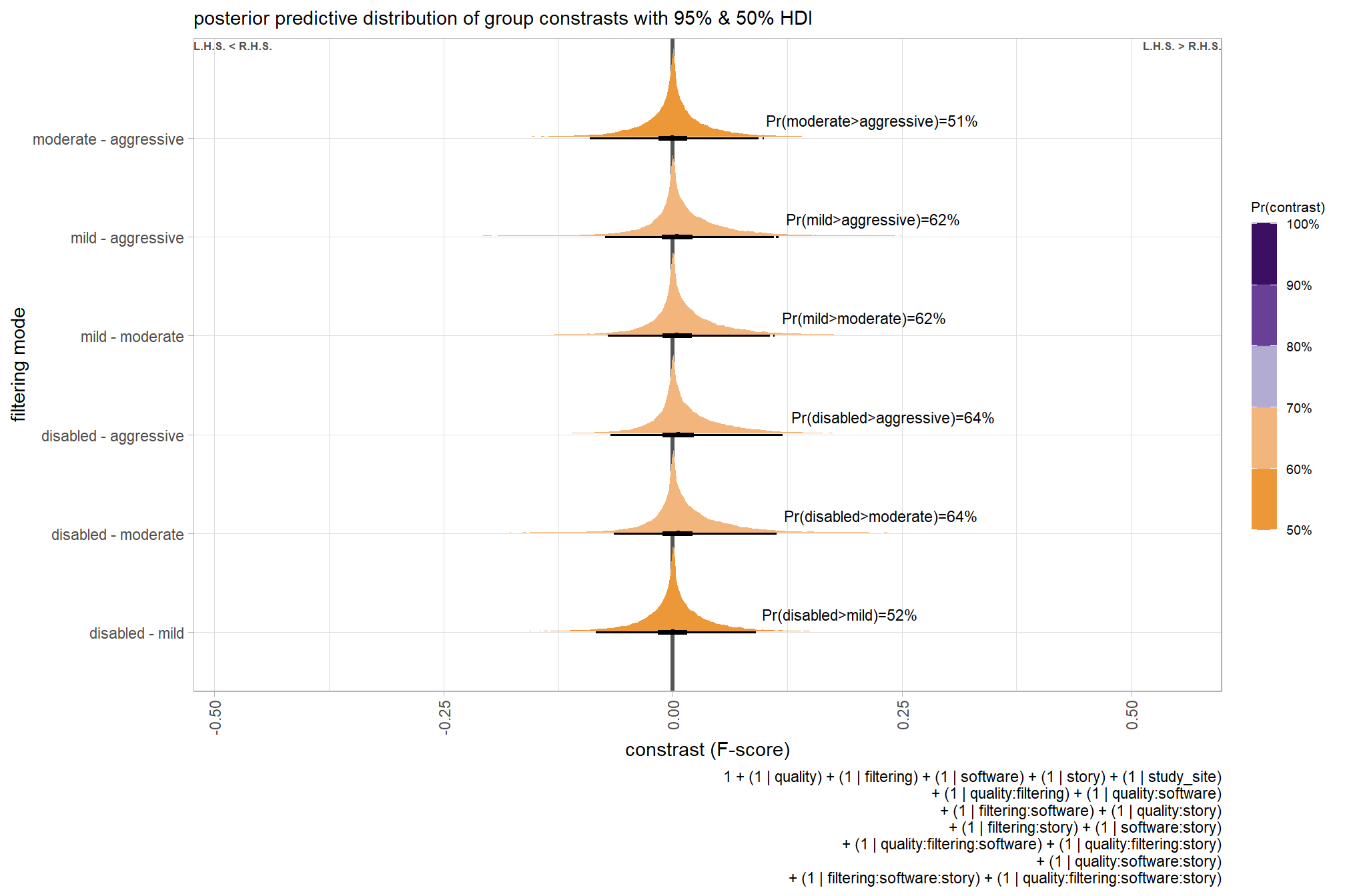
and summarize these contrasts
brms_contrast_temp %>%
dplyr::group_by(contrast, pr_gt_zero) %>%
tidybayes::median_hdi(value) %>%
dplyr::arrange(contrast) %>%
dplyr::select(contrast, value, .lower, .upper, pr_gt_zero) %>%
kableExtra::kbl(
digits = 2
, caption = "brms::brm model: 95% HDI of the posterior predictive distribution of group constrasts"
, col.names = c(
"filtering mode contrast"
, "difference (F-score)"
, "HDI low", "HDI high"
, "Pr(diff>0)"
)
) %>%
kableExtra::kable_styling()| filtering mode contrast | difference (F-score) | HDI low | HDI high | Pr(diff>0) |
|---|---|---|---|---|
| disabled - mild | 0.00 | -0.08 | 0.09 | 52% |
| disabled - moderate | 0.01 | -0.06 | 0.11 | 64% |
| disabled - aggressive | 0.01 | -0.07 | 0.12 | 64% |
| mild - moderate | 0.00 | -0.07 | 0.11 | 62% |
| mild - moderate | 0.00 | 0.11 | 0.11 | 62% |
| mild - aggressive | 0.01 | -0.08 | -0.08 | 62% |
| mild - aggressive | 0.01 | -0.07 | 0.11 | 62% |
| mild - aggressive | 0.01 | 0.11 | 0.12 | 62% |
| moderate - aggressive | 0.00 | -0.09 | 0.09 | 51% |
| moderate - aggressive | 0.00 | 0.10 | 0.10 | 51% |
6.9.2.10 Software - main effect
to address one of our main questions, let’s also collapse across the story, study site, dense cloud quality, and filtering mode setting to compare the software effect.
In a hierarchical model structure, we have to make use of the re_formula argument within tidybayes::add_epred_draws
ptcld_validation_data %>%
dplyr::distinct(software) %>%
tidybayes::add_epred_draws(
brms_f_mod6
# this part is crucial
, re_formula = ~ (1 | software)
) %>%
dplyr::rename(value = .epred) %>%
# plot
ggplot(
mapping = aes(
x = value, y = software
, fill = software
)
) +
tidybayes::stat_halfeye(
point_interval = median_hdi, .width = .95
, interval_color = "gray66"
, shape = 21, point_color = "gray66", point_fill = "black"
, justification = -0.01
) +
scale_fill_viridis_d(option = "rocket", begin = 0.3, end = 0.9, drop = F) +
scale_x_continuous(breaks = scales::extended_breaks(n=8)) +
labs(
y = "software", x = "F-score"
, subtitle = "posterior predictive distribution of F-score with 95% HDI"
, caption = form_temp
) +
theme_light() +
theme(legend.position = "none")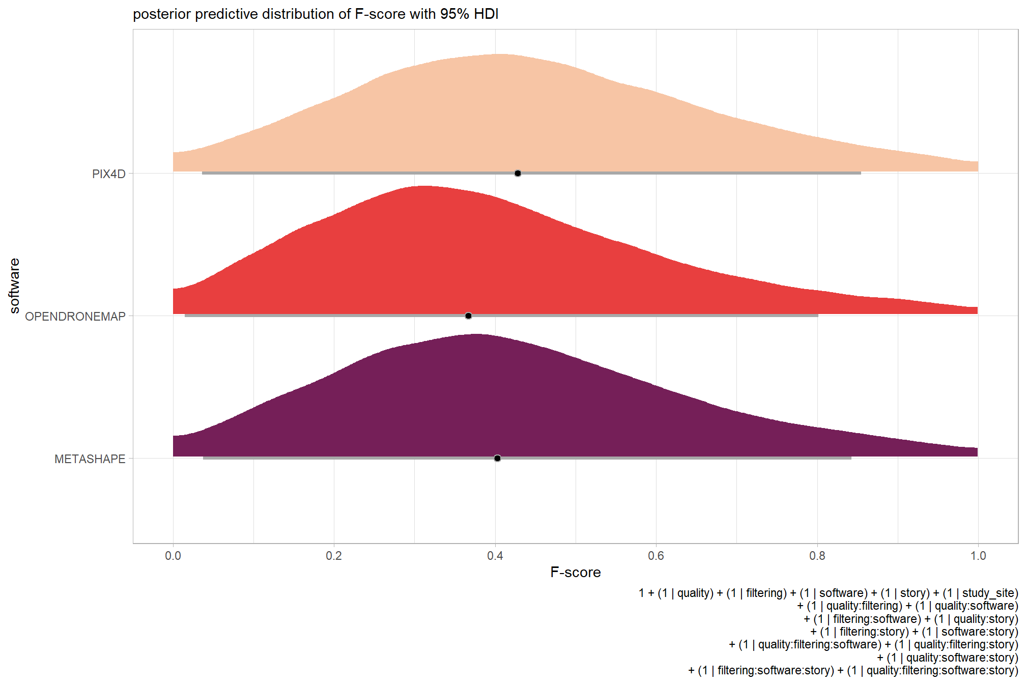
we can also perform pairwise comparisons
brms_contrast_temp =
ptcld_validation_data %>%
dplyr::distinct(software) %>%
tidybayes::add_epred_draws(
brms_f_mod6, allow_new_levels = T
# this part is crucial
, re_formula = ~ (1 | software)
) %>%
dplyr::rename(value = .epred) %>%
tidybayes::compare_levels(
value
, by = software
, comparison = "pairwise"
) %>%
dplyr::rename(contrast = software) %>%
# median_hdi summary for coloring
dplyr::group_by(contrast) %>%
make_contrast_vars()
# what?
brms_contrast_temp %>% dplyr::glimpse()## Rows: 120,000
## Columns: 16
## Groups: contrast [3]
## $ .chain <int> NA, NA, NA, NA, NA, NA, NA, NA, NA, NA, NA, NA, NA, N…
## $ .iteration <int> NA, NA, NA, NA, NA, NA, NA, NA, NA, NA, NA, NA, NA, N…
## $ .draw <int> 1, 2, 3, 4, 5, 6, 7, 8, 9, 10, 11, 12, 13, 14, 15, 16…
## $ contrast <chr> "OPENDRONEMAP - METASHAPE", "OPENDRONEMAP - METASHAPE…
## $ value <dbl> -9.337236e-02, 4.289334e-02, -5.244894e-02, -5.874655…
## $ median_hdi_est <dbl> -0.01532781, -0.01532781, -0.01532781, -0.01532781, -…
## $ median_hdi_lower <dbl> -0.2559431, -0.2559431, -0.2559431, -0.2559431, -0.25…
## $ median_hdi_upper <dbl> 0.1696568, 0.1696568, 0.1696568, 0.1696568, 0.1696568…
## $ pr_gt_zero <chr> "37%", "37%", "37%", "37%", "37%", "37%", "37%", "37%…
## $ pr_lt_zero <chr> "63%", "63%", "63%", "63%", "63%", "63%", "63%", "63%…
## $ is_diff_dir <lgl> TRUE, FALSE, TRUE, TRUE, TRUE, TRUE, TRUE, TRUE, FALS…
## $ pr_diff <dbl> 0.6325, 0.6325, 0.6325, 0.6325, 0.6325, 0.6325, 0.632…
## $ pr_diff_lab <chr> "Pr(MtaShp>ODM)=63%", "Pr(MtaShp>ODM)=63%", "Pr(MtaSh…
## $ pr_diff_lab_sm <chr> "Pr(<0)=63%", "Pr(<0)=63%", "Pr(<0)=63%", "Pr(<0)=63%…
## $ pr_diff_lab_pos <dbl> -0.2751388, -0.2751388, -0.2751388, -0.2751388, -0.27…
## $ sig_level <ord> <80%, <80%, <80%, <80%, <80%, <80%, <80%, <80%, <80%,…plot it
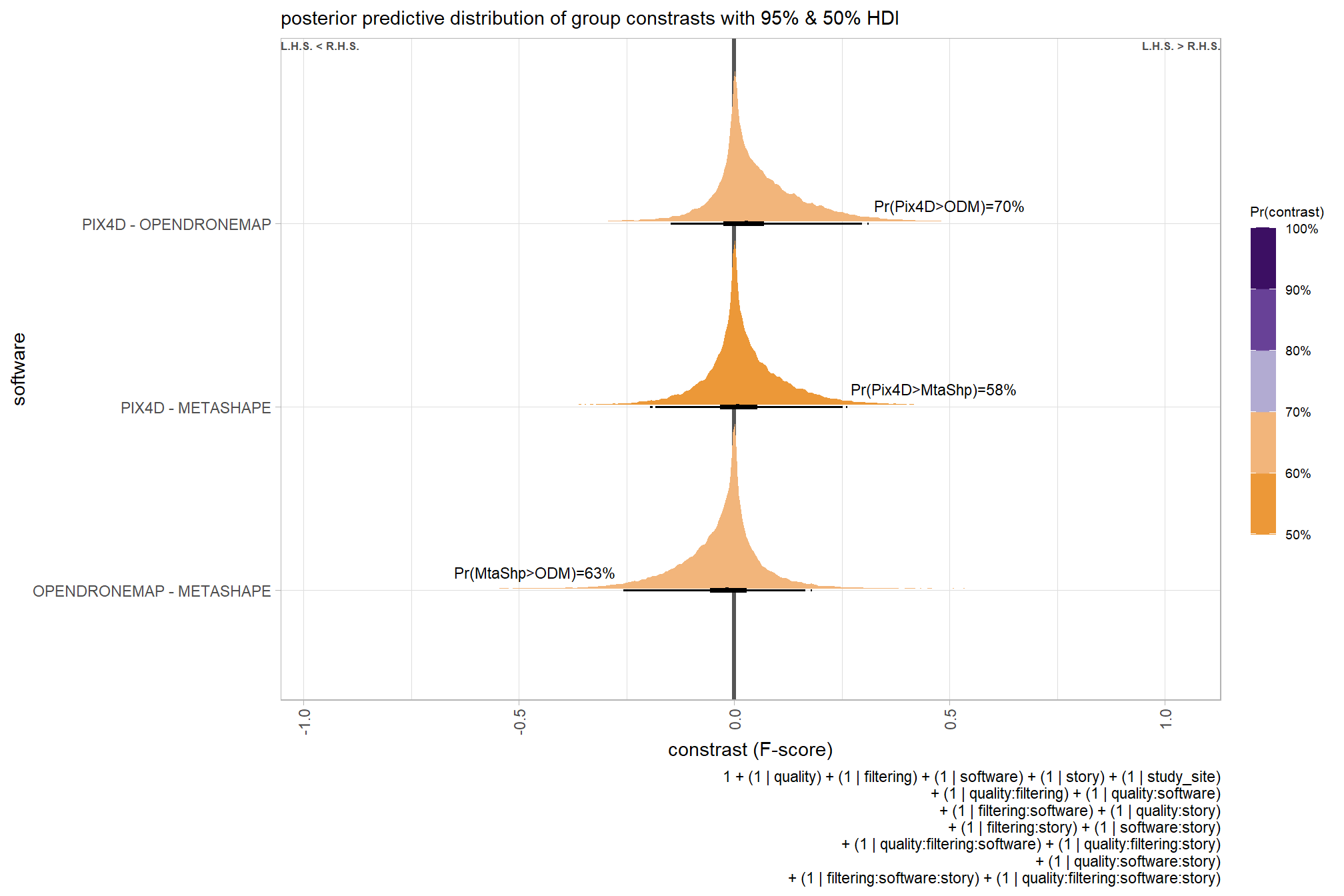
and summarize these contrasts
brms_contrast_temp %>%
dplyr::group_by(contrast, pr_gt_zero) %>%
tidybayes::median_hdi(value) %>%
dplyr::arrange(contrast) %>%
dplyr::select(contrast, value, .lower, .upper, pr_gt_zero) %>%
kableExtra::kbl(
digits = 2
, caption = "brms::brm model: 95% HDI of the posterior predictive distribution of group constrasts"
, col.names = c(
"software contrast"
, "difference (F-score)"
, "HDI low", "HDI high"
, "Pr(diff>0)"
)
) %>%
kableExtra::kable_styling()| software contrast | difference (F-score) | HDI low | HDI high | Pr(diff>0) |
|---|---|---|---|---|
| OPENDRONEMAP - METASHAPE | -0.02 | -0.26 | 0.17 | 37% |
| OPENDRONEMAP - METASHAPE | -0.02 | 0.18 | 0.18 | 37% |
| PIX4D - METASHAPE | 0.01 | -0.20 | -0.19 | 58% |
| PIX4D - METASHAPE | 0.01 | -0.18 | 0.25 | 58% |
| PIX4D - METASHAPE | 0.01 | 0.26 | 0.26 | 58% |
| PIX4D - OPENDRONEMAP | 0.03 | -0.15 | 0.30 | 70% |
| PIX4D - OPENDRONEMAP | 0.03 | 0.31 | 0.31 | 70% |
6.9.2.11 \(\sigma\) posteriors
Finally, we can quantify the variation in F-score by comparing the \(\sigma\) (sd) posteriors
unsure about the scale of the \(\sigma\) parameters are on in the beta model. Here, we invert the logit sd values from the model using plogis() which converts the parameter values to a probability/proportion (e.g.; 0-1) because they are parameters of the intercept and interaction effects so must be on the transformed (link = "logit") scale…double check
For a phenomenally excellent overview of binary logistic regression and how to interpret coefficients, see Steven Miller’s most excellent lab script here
# tidybayes::get_variables(brms_f_mod6)
# extract the posterior draws
brms::as_draws_df(brms_f_mod6) %>%
dplyr::select(c(tidyselect::starts_with("sd_"))) %>%
tidyr::pivot_longer(dplyr::everything()) %>%
# dplyr::group_by(name) %>%
# tidybayes::median_hdi(value) %>%
dplyr::mutate(
name = name %>%
stringr::str_replace_all("depth_maps_generation_quality", "quality") %>%
stringr::str_replace_all("depth_maps_generation_filtering_mode", "filtering") %>%
forcats::fct_reorder(value)
, value = plogis(value)
) %>%
# plot
ggplot(aes(x = value, y = name)) +
tidybayes::stat_dotsinterval(
point_interval = median_hdi, .width = .95
, justification = -0.04
, shape = 21 #, point_size = 3
, quantiles = 100
) +
labs(x = "", y = "", caption = form_temp) +
theme_light()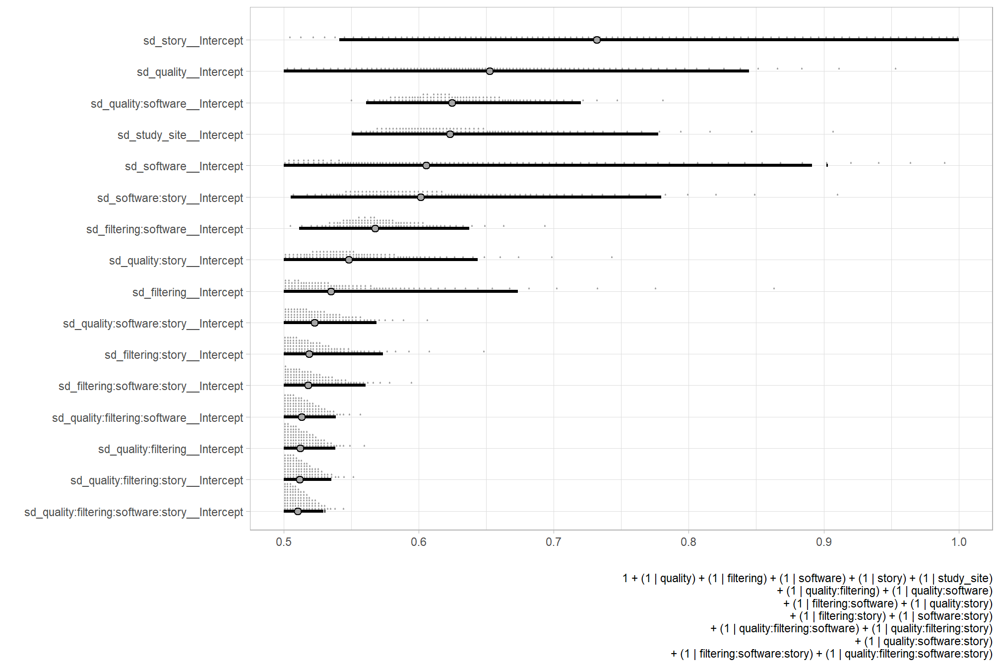
Determining overstory or understory seems to have the strongest effect on our ability to accurately detect trees but this effect is highly uncertain. Variance of study site is stronger than variance of depth map generation quality, but the posterior predictive distributions overlap a good deal. The study site (the “subjects” in our study) seems to have the overall strongest effect, but this comes with high uncertainty. Taken alone, the influence of quality, filtering, and software comes with huge uncertainty. This makes sense as the influence of software largely depends on the depth map generation quality, of which we are fairly certain. Filtering mode has the overall weakest effect on tree detection and this comes with relatively high certainty, especially conditional on the depth map generation quality.
and perform model selection via the R-squared for Bayesian regression models using brms::bayes_R2() since we can’t compare models with different number of observations using information criteria (we could also use the p-value approach as done above)
brms_f_mod6 = brms::add_criterion(brms_f_mod6, criterion = c("loo", "waic"))
# r-squared
dplyr::bind_rows(
brms::bayes_R2(brms_f_mod6) %>% dplyr::as_tibble() %>% dplyr::mutate(model = "brms_f_mod6") %>% dplyr::relocate(model)
, brms::bayes_R2(brms_f_mod5) %>% dplyr::as_tibble() %>% dplyr::mutate(model = "brms_f_mod5") %>% dplyr::relocate(model)
) %>%
dplyr::rename_with(tolower) %>%
dplyr::arrange(desc(estimate)) %>%
dplyr::rename(R2.estimate = estimate)## # A tibble: 2 × 5
## model R2.estimate est.error q2.5 q97.5
## <chr> <dbl> <dbl> <dbl> <dbl>
## 1 brms_f_mod5 0.664 0.0248 0.610 0.707
## 2 brms_f_mod6 0.573 0.0204 0.530 0.610Our model without the effects of overstory/understory is a better parsimonious fit of the data in this case…let’s roll with brms_f_mod5 model for the research article even though our model including overstory/understory has less dispersion (see our \(\phi\) posterior)