Section 3 R Point Cloud Processing
After running the UAS point cloud processing script in R…the processing tracking data file is used to compare summary statistics on point cloud processing times.
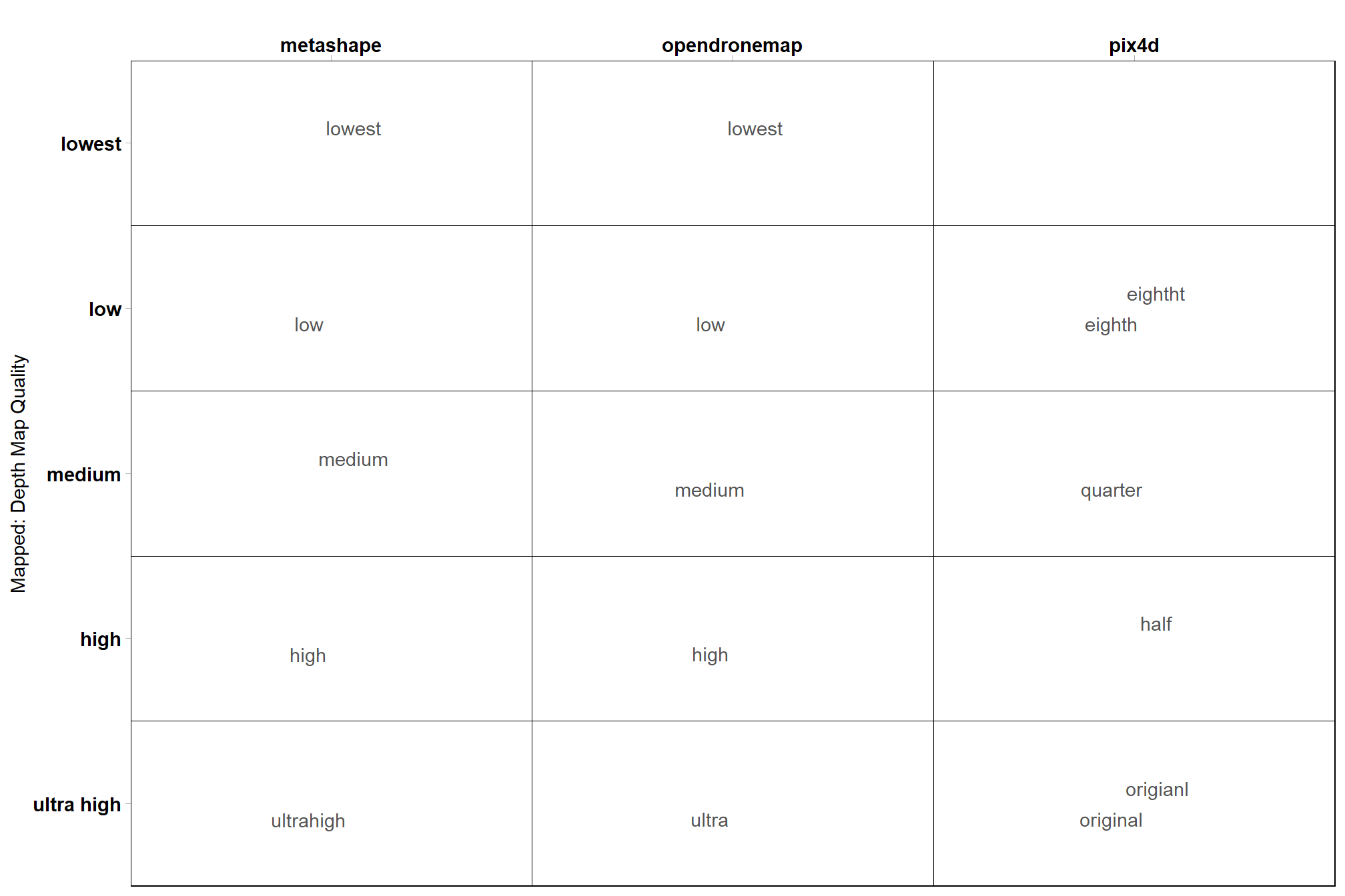
For comparison across software, the SfM point cloud generation processing parameters are mapped to the Metashape parameters based on the Pix4D documentation, the OpenDroneMap documentation, and the Agisoft Metashape discussion board
### get tracking data
# read list of all processed tracking files
tracking_list_df =
dplyr::tibble(
file_full_path = list.files(
ptcld_processing_dir
, pattern = ".*_processed_tracking_data\\.csv$"
, full.names = T, recursive = T
) %>%
normalizePath()
) %>%
# get the software used
dplyr::mutate(
file_full_path %>%
toupper() %>%
stringr::str_extract_all(pattern = paste(toupper(software_list),collapse = "|"), simplify = T) %>%
dplyr::as_tibble() %>%
tidyr::unite(col = "software", sep = " ", na.rm = T)
) %>%
# filter processed tracking files
dplyr::mutate(
software = software %>% stringr::word(-1)
, study_site = file_full_path %>%
toupper() %>%
stringr::str_extract(pattern = paste(toupper(study_site_list),collapse = "|"))
, file_name = file_full_path %>%
basename() %>%
stringr::word(1, sep = fixed(".")) %>%
toupper() %>%
stringr::str_remove_all("_PROCESSED_TRACKING_DATA")
) %>%
dplyr::filter(
!is.na(study_site)
& study_site %in% toupper(study_site_list)
& !is.na(software)
& software %in% toupper(software_list)
) %>%
# keep only unique files for processing
dplyr::group_by(software, study_site, file_name) %>%
dplyr::filter(dplyr::row_number()==1) %>%
dplyr::ungroup() %>%
dplyr::rename(tracking_file_full_path = file_full_path)
# tracking_list_df %>% dplyr::glimpse()
# read each tracking data file, bind rows
ptcld_processing_data = 1:nrow(tracking_list_df) %>%
purrr::map(function(row_n){
tracking_list_df %>%
dplyr::filter(dplyr::row_number() == row_n) %>%
dplyr::bind_cols(
read.csv(tracking_list_df$tracking_file_full_path[row_n])
)
}) %>%
dplyr::bind_rows()
# ptcld_processing_data %>% dplyr::glimpse()
# split file name to get processing attributes
ptcld_processing_data =
ptcld_processing_data %>%
tidyr::separate_wider_delim(
cols = file_name
, delim = "_"
, names = paste0(
"processing_attribute"
, 1:(max(stringr::str_count(ptcld_processing_data$file_name, "_"))+1)
)
, too_few = "align_start"
, cols_remove = F
) %>%
# not sure how to map processing attributes for pix4d and opendronemap ??????????????
dplyr::mutate(
# temporary
qqq = dplyr::case_when(
tolower(software) == "pix4d" ~ processing_attribute2
, T ~ processing_attribute1
)
, fff = dplyr::case_when(
tolower(software) == "pix4d" ~ processing_attribute3
, T ~ processing_attribute2
)
# mapping
, depth_maps_generation_quality = dplyr::case_when(
tolower(qqq) %in% c("ultrahigh", "ultra", "original", "origianl") ~ "ultra high"
, tolower(qqq) %in% c("half") ~ "high"
, tolower(qqq) %in% c("quarter") ~ "medium"
, tolower(qqq) %in% c("eighth","eightht") ~ "low"
, T ~ tolower(qqq)
) %>%
factor(
ordered = TRUE
, levels = c(
"lowest"
, "low"
, "medium"
, "high"
, "ultra high"
)
) %>% forcats::fct_rev()
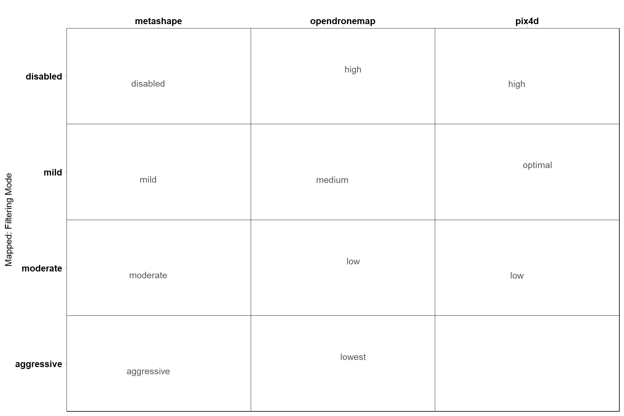
, depth_maps_generation_filtering_mode = dplyr::case_when(
tolower(fff) %in% c("high") &
tolower(software) %in% c("opendronemap") ~ "disabled"
, tolower(fff) %in% c("high")
& tolower(software) %in% c("pix4d") ~ "disabled"
, tolower(fff) %in% c("medium")
& tolower(software) %in% c("opendronemap") ~ "mild"
, tolower(fff) %in% c("optimal")
& tolower(software) %in% c("pix4d") ~ "mild"
, tolower(fff) %in% c("low")
& tolower(software) %in% c("opendronemap") ~ "moderate"
, tolower(fff) %in% c("low")
& tolower(software) %in% c("pix4d") ~ "moderate"
, tolower(fff) %in% c("lowest")
& tolower(software) %in% c("opendronemap") ~ "aggressive"
, T ~ tolower(fff)
) %>%
factor(
ordered = TRUE
, levels = c(
"disabled"
, "mild"
, "moderate"
, "aggressive"
)
) %>% forcats::fct_rev()
)what have we done?
## Rows: 500
## Columns: 33
## $ tracking_file_full_path              <chr> "D:\\SfM_Software_Comparison\\Met…
## $ software                             <chr> "METASHAPE", "METASHAPE", "METASH…
## $ study_site                           <chr> "KAIBAB_HIGH", "KAIBAB_HIGH", "KA…
## $ processing_attribute1                <chr> "HIGH", "HIGH", "HIGH", "HIGH", "…
## $ processing_attribute2                <chr> "AGGRESSIVE", "DISABLED", "MILD",…
## $ processing_attribute3                <chr> NA, NA, NA, NA, NA, NA, NA, NA, N…
## $ file_name                            <chr> "HIGH_AGGRESSIVE", "HIGH_DISABLED…
## $ number_of_points                     <int> 52974294, 72549206, 69858217, 698…
## $ las_area_m2                          <dbl> 86661.27, 87175.42, 86404.78, 864…
## $ timer_tile_time_mins                 <dbl> 0.63600698, 2.49318542, 0.8413380…
## $ timer_class_dtm_norm_chm_time_mins   <dbl> 3.6559556, 5.3289152, 5.1638296, …
## $ timer_treels_time_mins               <dbl> 8.9065272, 19.2119663, 12.3391793…
## $ timer_itd_time_mins                  <dbl> 0.02202115, 0.02449968, 0.0379844…
## $ timer_competition_time_mins          <dbl> 0.10590740, 0.17865245, 0.1212486…
## $ timer_estdbh_time_mins               <dbl> 0.02290262, 0.02382533, 0.0219917…
## $ timer_silv_time_mins                 <dbl> 0.012565533, 0.015940932, 0.01503…
## $ timer_total_time_mins                <dbl> 13.361886, 27.276985, 18.540606, …
## $ sttng_input_las_dir                  <chr> "D:/Metashape_Testing_2024", "D:/…
## $ sttng_use_parallel_processing        <lgl> FALSE, FALSE, FALSE, FALSE, FALSE…
## $ sttng_desired_chm_res                <dbl> 0.25, 0.25, 0.25, 0.25, 0.25, 0.2…
## $ sttng_max_height_threshold_m         <int> 60, 60, 60, 60, 60, 60, 60, 60, 6…
## $ sttng_minimum_tree_height_m          <int> 2, 2, 2, 2, 2, 2, 2, 2, 2, 2, 2, …
## $ sttng_dbh_max_size_m                 <int> 2, 2, 2, 2, 2, 2, 2, 2, 2, 2, 2, …
## $ sttng_local_dbh_model                <chr> "rf", "rf", "rf", "rf", "rf", "rf…
## $ sttng_user_supplied_epsg             <lgl> NA, NA, NA, NA, NA, NA, NA, NA, N…
## $ sttng_accuracy_level                 <int> 2, 2, 2, 2, 2, 2, 2, 2, 2, 2, 2, …
## $ sttng_pts_m2_for_triangulation       <int> 20, 20, 20, 20, 20, 20, 20, 20, 2…
## $ sttng_normalization_with             <chr> "triangulation", "triangulation",…
## $ sttng_competition_buffer_m           <int> 5, 5, 5, 5, 5, 5, 5, 5, 5, 5, 5, …
## $ qqq                                  <chr> "HIGH", "HIGH", "HIGH", "HIGH", "…
## $ fff                                  <chr> "AGGRESSIVE", "DISABLED", "MILD",…
## $ depth_maps_generation_quality        <ord> high, high, high, high, low, low,…
## $ depth_maps_generation_filtering_mode <ord> aggressive, disabled, mild, moder…
what is this mapping?
# quality
ptcld_processing_data %>%
  dplyr::count(depth_maps_generation_quality, qqq, software) %>%
  ggplot(aes(x = tolower(software), y = depth_maps_generation_quality, label = tolower(qqq))) +
    geom_tile(fill = NA, color = "black") +
    ggrepel::geom_text_repel(color = "gray33") +
    labs(y = "Mapped: Depth Map Quality", x = "") +
    scale_x_discrete(position = "top") +
    coord_cartesian(expand = F) +
    theme_light() +
    theme(
      panel.grid = element_blank()
      , axis.text = element_text(size = 11, face = "bold", color = "black")
      , panel.border = element_rect(color = "black")
    )
# filtering
ptcld_processing_data %>%
  dplyr::count(depth_maps_generation_filtering_mode, fff, software) %>%
  ggplot(aes(x = tolower(software), y = depth_maps_generation_filtering_mode, label = tolower(fff))) +
    geom_tile(fill = NA, color = "black") +
    ggrepel::geom_text_repel(color = "gray33") +
    labs(y = "Mapped: Filtering Mode", x = "") +
    scale_x_discrete(position = "top") +
    coord_cartesian(expand = F) +
    theme_light() +
    theme(
      panel.grid = element_blank()
      , axis.text = element_text(size = 11, face = "bold", color = "black")
      , panel.border = element_rect(color = "black")
    )
# !!!!!!!!!!!!!!!!!!!!!!!!!!!!!!!!!!!! Filtering
# !!!! keep only one kind of pix4d, all metashape and odm ???????
ptcld_processing_data = ptcld_processing_data %>%
  dplyr::select(-c(qqq,fff)) %>%
  dplyr::filter(
    dplyr::case_when(
      tolower(software) == "pix4d" & tolower(processing_attribute1) == "original" ~ T
      , tolower(software) != "pix4d" ~ T
      , T ~ F
    ) == T
  )
3.1 ODM and Pix4D Image Processing
This piece really belongs in the previous section on SfM Image Processing Data…but we need to match manual Excel data with the data structure we created immediately above just to make a figure on image processing time for publication even though the softwares were all run on different machines which means we need to figure out a way to standardize the image processing time to compare across software
For ODM and Pix4D, the image processing (SfM algorithm) time was compiled manually and stored in an Excel ;/ worksheet with the Total Generation Time (min) column tracking the processing time.
load the Excel file
odm_pix_temp = readxl::read_xlsx("../data/SfM_Processing_Time.xlsx") %>%
  dplyr::rename_with(~ .x %>%
    stringr::str_squish() %>%
    str_remove_all("[[:punct:]]") %>%
    stringr::str_replace_all("\\s","_") %>%
    tolower()
  ) %>%
  # map the processing parameters to the columns in our current data str
  dplyr::mutate(
    software = software %>%
      stringr::str_remove_all("\\s") %>%
      toupper()
    , processing_attribute1 = dplyr::case_when(
        software == "PIX4D" ~ keypoint_image_scale
        , T ~ depth_map_quality
      )
    , processing_attribute2 = dplyr::case_when(
        software == "PIX4D" ~ depth_map_quality
        , T ~ filtering_mode
      )
    , processing_attribute3 = dplyr::case_when(
        software == "PIX4D" ~ filtering_mode
        , T ~ as.character(NA)
      )
  ) %>%
  # clean the data
  dplyr::mutate(
    dplyr::across(
      tidyselect::starts_with("processing_attribute")
      , ~ .x %>%
        stringr::str_remove_all("\\s") %>%
        toupper()
    )
    , site = site %>%
      stringr::str_squish() %>%
      stringr::str_replace_all("\\s","_") %>%
      stringr::str_replace_all("[^[:alnum:]]","_") %>%
      toupper()
  ) %>%
  # filter pix4d like above
  dplyr::filter(
    dplyr::case_when(
      tolower(software) == "pix4d" & tolower(processing_attribute1) == "original" ~ T
      , tolower(software) != "pix4d" ~ T
      , T ~ F
    ) == T
  ) %>%
  # follow the same mapping of the processing attributes used above
  # ... would prefer to join by the processing_attribute columns, but some of the
  # ... values are mislabeled such as "eighth" and "origianl"
  # not sure how to map processing attributes for pix4d and opendronemap ??????????????
  dplyr::mutate(
    # temporary
    qqq = dplyr::case_when(
        tolower(software) == "pix4d" ~ processing_attribute2
        , T ~ processing_attribute1
      )
    , fff = dplyr::case_when(
        tolower(software) == "pix4d" ~ processing_attribute3
        , T ~ processing_attribute2
      )
  ) %>%
  dplyr::rename(
    study_site = site
    , total_sfm_time_min = total_generation_time_min
    , number_of_points_sfm = pc_total_number
  ) %>%
  # select columns we need for joining
  dplyr::select(
    software
    , study_site
    , total_sfm_time_min
    , number_of_points_sfm
    , qqq
    , fff
  )
clean up the metashape image processing data and combine with odm and pix4d
# clean up the metashape image processing data and combine with odm and pix4d
sfm_comb_temp = pdf_list_df %>%
  dplyr::mutate(
    software = toupper("metashape")
    , total_sfm_time_min =
      total_dense_point_cloud_processing_time_mins +
      total_sparse_point_cloud_processing_time_mins
    , number_of_points_sfm = dense_point_cloud_points
    , qqq = metashape_quality
    , fff = metashape_depthmap_filtering
  ) %>%
  dplyr::select(names(odm_pix_temp)) %>%
  dplyr::bind_rows(odm_pix_temp) %>%
  # map quality and filtering to match above
  dplyr::mutate(
    # mapping
    depth_maps_generation_quality = dplyr::case_when(
        tolower(qqq) %in% c("ultrahigh", "ultra", "original", "origianl") ~ "ultra high"
        , tolower(qqq) %in% c("half") ~ "high"
        , tolower(qqq) %in% c("quarter") ~ "medium"
        , tolower(qqq) %in% c("eighth","eightht") ~ "low"
        , T ~ tolower(qqq)
      ) %>%
      factor(
        ordered = TRUE
        , levels = c(
          "lowest"
          , "low"
          , "medium"
          , "high"
          , "ultra high"
        )
      ) %>% forcats::fct_rev()
    , depth_maps_generation_filtering_mode = dplyr::case_when(
        tolower(fff) %in% c("high") &
          tolower(software) %in% c("opendronemap") ~ "disabled"
        , tolower(fff) %in% c("high")
          & tolower(software) %in% c("pix4d") ~ "disabled"
        , tolower(fff) %in% c("medium")
          & tolower(software) %in% c("opendronemap") ~ "mild"
        , tolower(fff) %in% c("optimal")
          & tolower(software) %in% c("pix4d") ~ "mild"
        , tolower(fff) %in% c("low")
          & tolower(software) %in% c("opendronemap") ~ "moderate"
        , tolower(fff) %in% c("low")
          & tolower(software) %in% c("pix4d") ~ "moderate"
        , tolower(fff) %in% c("lowest")
          & tolower(software) %in% c("opendronemap") ~ "aggressive"
        , T ~ tolower(fff)
      ) %>%
      factor(
        ordered = TRUE
        , levels = c(
          "disabled"
          , "mild"
          , "moderate"
          , "aggressive"
        )
      ) %>% forcats::fct_rev()
  ) %>%
  dplyr::select(-c(qqq,fff)) %>%
  # keep only one thing record
  dplyr::group_by(
    software, study_site, depth_maps_generation_quality, depth_maps_generation_filtering_mode
  ) %>%
  dplyr::filter(dplyr::row_number()==1) %>%
  dplyr::ungroup()
join to the processing data which we’ll use to build our full analysis data set and create the normalized processing time using Min-Max normalization as:
\[ x^{\prime}_{ij} = \frac{x_{ij}-x_{min[j]}}{x_{max[j]}-x_{min[j]}} \]
where \(i\) is the the study site observation within each software \(j\) where each software was implemented on a different computer.
ptcld_processing_data = ptcld_processing_data %>%
dplyr::left_join(
sfm_comb_temp
, by = dplyr::join_by(
software, study_site, depth_maps_generation_quality, depth_maps_generation_filtering_mode
)
) %>%
# create the standardized time by software since the processing machine varied by software
dplyr::group_by(software) %>%
dplyr::mutate(
total_sfm_time_norm = (total_sfm_time_min-min(total_sfm_time_min, na.rm = T)) /
(max(total_sfm_time_min, na.rm = T)-min(total_sfm_time_min, na.rm = T))
) %>%
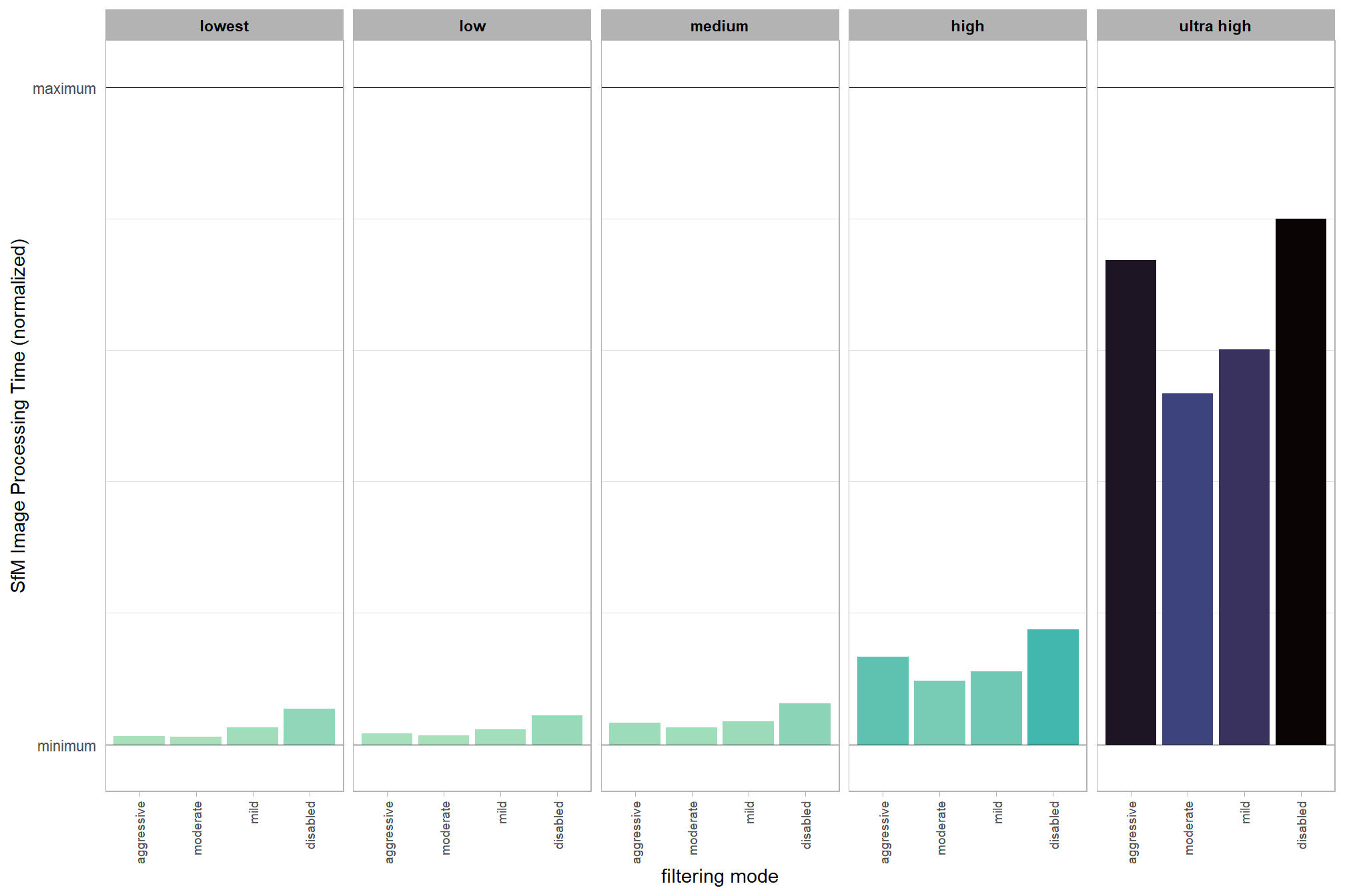
dplyr::ungroup()quick summary of the normalized SfM processing time
ptcld_processing_data %>%
  dplyr::group_by(depth_maps_generation_quality, depth_maps_generation_filtering_mode) %>%
  dplyr::summarise(total_sfm_time_norm = mean(total_sfm_time_norm)) %>%
  dplyr::mutate(depth_maps_generation_quality = forcats::fct_rev(depth_maps_generation_quality)) %>%
  ggplot(mapping = aes(
    x = depth_maps_generation_filtering_mode
    , y = total_sfm_time_norm
    , fill = total_sfm_time_norm
  )) +
    geom_col() +
    facet_grid(cols = vars(depth_maps_generation_quality)) +
    scale_fill_viridis_c(option = "mako", direction = -1, end = 0.9) +
    scale_y_continuous(
      limits = c(-0.02,1.02)
      , breaks = c(0, 1)
      , minor_breaks = seq(0.2,0.8,0.2)
      , labels = c("minimum","maximum")
    ) +
    labs(x = "filtering mode", y = "SfM Image Processing Time (normalized)") +
    theme_light() +
    theme(
      legend.position = "none"
      , legend.direction  = "horizontal"
      , panel.grid.major.x = element_blank()
      , panel.grid.minor.x = element_blank()
      , panel.grid.major.y = element_line(color = "black")
      , axis.ticks.y = element_blank()
      , axis.text.x = element_text(angle = 90, vjust = 0.5, hjust = 1, size = 7)
      , strip.text = element_text(color = "black", face = "bold")
      , plot.subtitle = element_text(hjust = 0.5)
    )
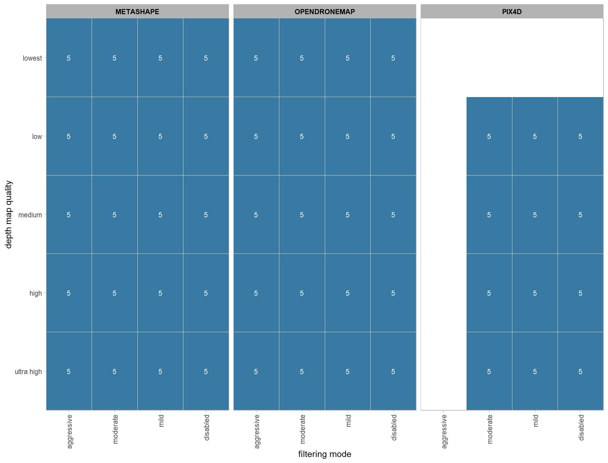
3.2 Number of files summary
ptcld_processing_data %>%
  dplyr::count(software, depth_maps_generation_quality, depth_maps_generation_filtering_mode) %>%
  ggplot(mapping = aes(
    y = depth_maps_generation_quality
    , x = depth_maps_generation_filtering_mode
    , fill = n
    , label = n
  )) +
  geom_tile(color = "white") +
  geom_text(color = "white", size = 3) +
  facet_grid(cols = vars(software)) +
  scale_x_discrete(expand = c(0, 0)) +
  scale_y_discrete(expand = c(0, 0)) +
  scale_fill_viridis_c(option = "mako", direction=-1, begin = 0.2, end = 0.8) +
  labs(
    x = "filtering mode"
    , y = "depth map quality"
    , fill = "number of sites"
  ) +
  theme_light() +
  theme(
    legend.position = "none"
    , axis.text.x = element_text(angle = 90, vjust = 0.5, hjust = 1)
    , panel.background = element_blank()
    , panel.grid = element_blank()
    , plot.subtitle = element_text(hjust = 0.5)
    , strip.text = element_text(color = "black", face = "bold")
  )
3.3 Processing Time Summary
Total processing time by depth map generation quality and depth map filtering mode
ptcld_processing_data %>%
  ggplot(
    mapping = aes(
      x = depth_maps_generation_quality
      , y = timer_total_time_mins
      , color = depth_maps_generation_filtering_mode
      , fill = depth_maps_generation_filtering_mode
    )
  ) +
  geom_boxplot(alpha = 0.6) +
  scale_color_viridis_d(option = "plasma") +
  scale_fill_viridis_d(option = "plasma") +
  scale_y_log10(
    labels = scales::comma_format(suffix = " mins", accuracy = 1)
    , breaks = scales::breaks_log(n = 9)
  ) +
  labs(
    color = "Filtering Mode"
    , fill = "Filtering Mode"
    , y = "Point Cloud Total Processing Time"
    , x = "Quality"
    , title = bquote(
        bold("R") ~
        "point cloud total processing time by depth map generation quality and filtering mode"
    )
    , caption = "*Note the log scale on the y-axis"
  ) +
  theme_light() +
  theme(
    legend.position = "top"
    , legend.direction  = "horizontal"
  ) +
  guides(
    color = guide_legend(override.aes = list(shape = 15, size = 6, alpha = 0.9))
  )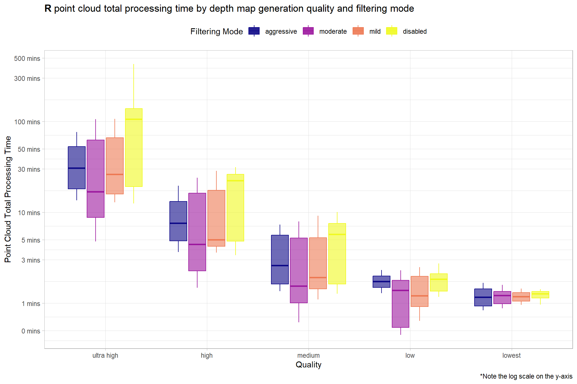
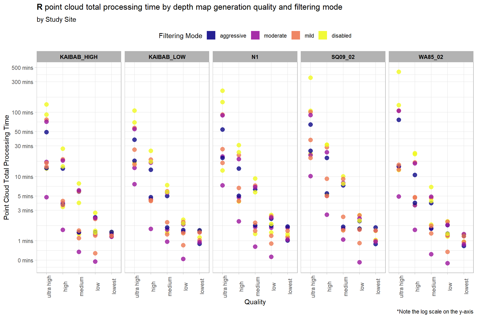
Notice there are some outlier study sites in the point cloud processing time
ptcld_processing_data %>%
  ggplot(
    mapping = aes(
      y = timer_total_time_mins
      , x = depth_maps_generation_quality
      , color = depth_maps_generation_filtering_mode
    )
  ) +
  geom_point(size = 3, alpha = 0.8) +
  facet_grid(
    cols = vars(study_site)
    , labeller = label_wrap_gen(width = 35, multi_line = TRUE)
  ) +
  scale_color_viridis_d(option = "plasma") +
  scale_y_log10(
    labels = scales::comma_format(suffix = " mins", accuracy = 1)
    , breaks = scales::breaks_log(n = 9)
  ) +
  labs(
    color = "Filtering Mode"
    , y = "Point Cloud Total Processing Time"
    , x = "Quality"
    , title = bquote(
        bold("R") ~
        "point cloud total processing time by depth map generation quality and filtering mode"
    )
    , subtitle = "by Study Site"
    , caption = "*Note the log scale on the y-axis"
  ) +
  theme_light() +
  theme(
    legend.position = "top"
    , legend.direction  = "horizontal"
    , strip.text = element_text(color = "black", face = "bold")
    , axis.text.x = element_text(angle = 90)
  ) +
  guides(
    color = guide_legend(override.aes = list(shape = 15, size = 6, alpha = 0.9))
  )
3.4 Processing Time vs # Points
ptcld_processing_data %>%
  ggplot(
    mapping = aes(
      x = number_of_points
      , y = timer_total_time_mins
    )
  ) +
  geom_point(alpha = 0.7, color = "navy") +
  scale_y_log10(
    labels = scales::comma_format(suffix = " mins", accuracy = 1)
    , breaks = scales::breaks_log(n = 9)
  ) +
  scale_x_log10(
    labels = scales::comma_format(suffix = " M", scale = 1e-6, accuracy = 1)
    , breaks = scales::breaks_log(n = 6)
  ) +
  labs(
    y = "Point Cloud Total Processing Time"
    , x = "Dense Point Cloud # Points"
    , title = bquote(
        bold("R") ~
        "point cloud total processing time versus dense point cloud number of points"
    )
    , caption = "*Note the log scale on both axes"
  ) +
  theme_light()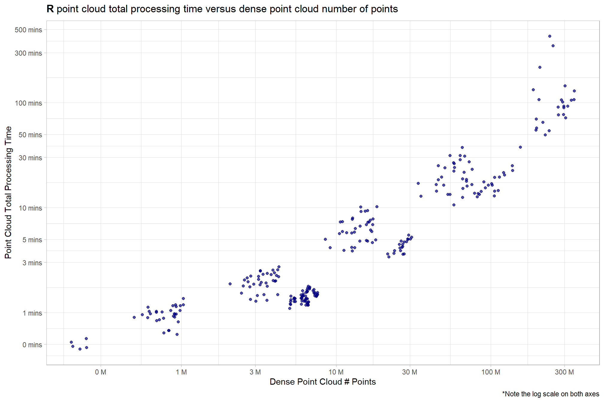
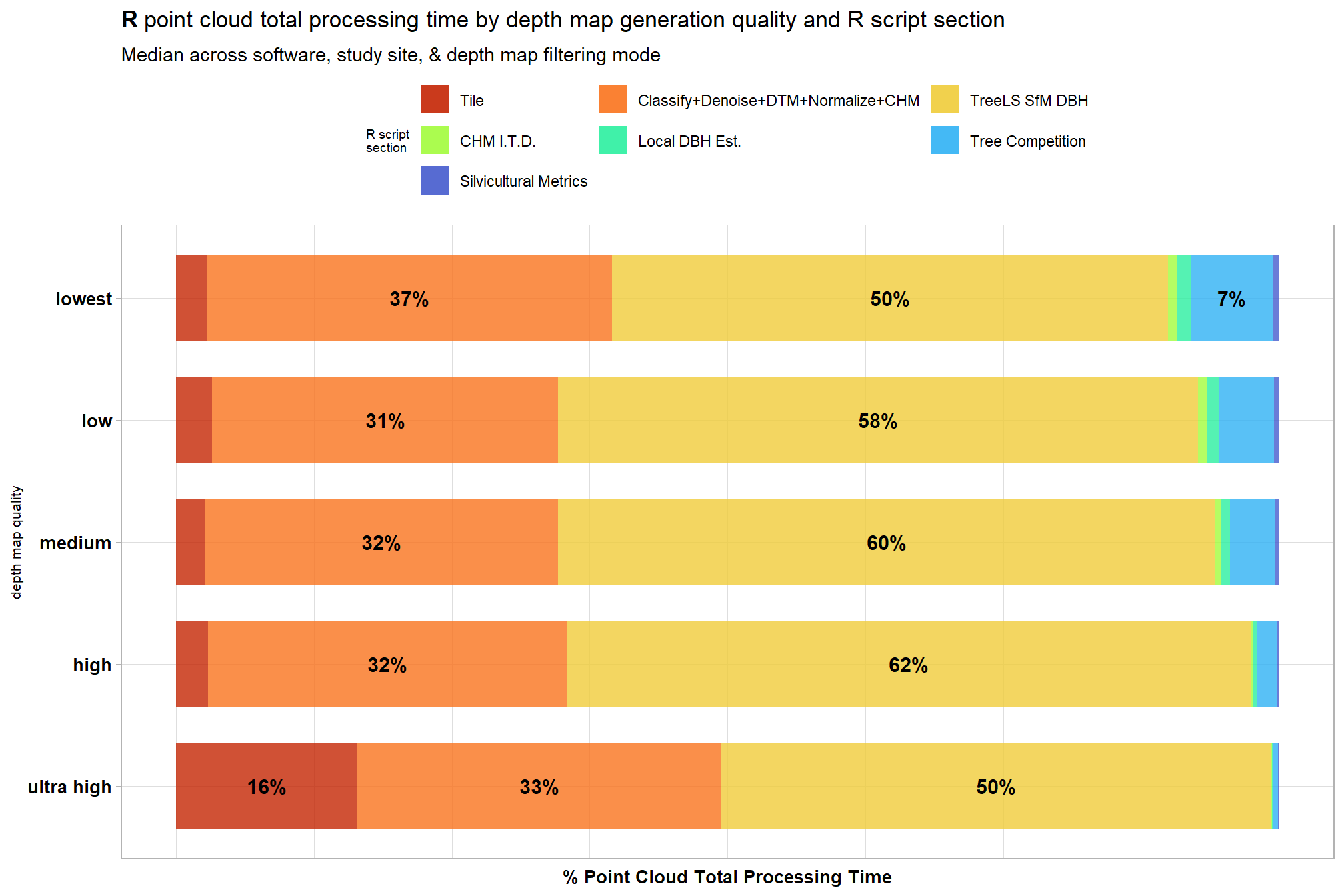
3.5 Processing Section Timing
ptcld_processing_data %>%
  dplyr::select(
    depth_maps_generation_quality
    , tidyselect::ends_with("_mins")
  ) %>%
  dplyr::select(-c(timer_total_time_mins)) %>%
  tidyr::pivot_longer(
    cols = -c(depth_maps_generation_quality)
    , names_to = "section"
    , values_to = "mins"
  ) %>%
  # dplyr::count(depth_maps_generation_quality, section)
  dplyr::group_by(depth_maps_generation_quality, section) %>%
  dplyr::summarise(med_mins = median(mins)) %>%
  dplyr::group_by(depth_maps_generation_quality) %>%
  dplyr::mutate(
    total_mins = sum(med_mins)
    , pct_mins = med_mins/total_mins
  ) %>%
  dplyr::ungroup() %>%
  dplyr::mutate(
    section = section %>%
      stringr::str_remove_all("timer_") %>%
      stringr::str_remove_all("_time_mins") %>%
      factor(
        ordered = T
        , levels = c(
          "tile"
          , "class_dtm_norm_chm"
          , "treels"
          , "itd"
          , "estdbh"
          , "competition"
          , "silv"
          ## olde
          # "tile"
          # , "denoise"
          # , "classify"
          # , "dtm"
          # , "normalize"
          # , "chm"
          # , "treels"
          # , "itd"
          # , "estdbh"
          # , "competition"
          # , "silv"
        )
        , labels = c(
          "Tile"
          , "Classify+Denoise+DTM+Normalize+CHM"
          , "TreeLS SfM DBH"
          , "CHM I.T.D."
          , "Local DBH Est."
          , "Tree Competition"
          , "Silvicultural Metrics"
        )
      ) %>% forcats::fct_rev()
  ) %>%

ggplot(
  mapping = aes(x = pct_mins, y = depth_maps_generation_quality, fill=section, group=section)
) +
  geom_col(
    width = 0.7, alpha=0.8
  ) +
  geom_text(
    mapping = aes(
        label = scales::percent(ifelse(pct_mins>=0.06,pct_mins,NA), accuracy = 1)
        , fontface = "bold"
      )
    , position = position_stack(vjust = 0.5)
    , color = "black", size = 4
  ) +
  scale_fill_viridis_d(option = "turbo", begin = 0.1, end = 0.9) +
  scale_x_continuous(labels = scales::percent_format()) +
  labs(
    fill = "R script\nsection"
    , y = "depth map quality"
    , x = "% Point Cloud Total Processing Time"
    , title = bquote(
        bold("R") ~
        "point cloud total processing time by depth map generation quality and R script section"
    )
    , subtitle = "Median across software, study site, & depth map filtering mode "
  ) +
  theme_light() +
  theme(
    legend.position = "top"
    , legend.direction  = "horizontal"
    , legend.title = element_text(size=7)
    , axis.title.x = element_text(size=10, face = "bold")
    , axis.title.y = element_text(size = 8)
    , axis.text.x = element_blank()
    , axis.text.y = element_text(color = "black",size=10, face = "bold")
    , axis.ticks.x = element_blank()
  ) +
  guides(
    fill = guide_legend(nrow = 3, byrow = T, reverse = T, override.aes = list(alpha = 0.9))
) 
3.6 Summary of point cloud data
Use flight boundary to calculate the per ha metrics but all of the flight boundaries based on the SfM data are different ; so will just use the Metashape “high” quality area median across filtering modes applied to all.
3.6.1 Table
table_temp =
  ptcld_processing_data %>%
  dplyr::select(
    # unique vars
    software, tidyselect::starts_with("depth_maps"), study_site
    # vars
    , number_of_points, timer_total_time_mins
  ) %>%
  # add area
  dplyr::inner_join(
    ptcld_processing_data %>%
      dplyr::mutate(
        las_area_m2 = dplyr::case_when(
          tolower(software)=="metashape"
            & tolower(depth_maps_generation_quality)=="high" ~ las_area_m2
          , T ~ NA
        )
      ) %>%
      dplyr::group_by(study_site) %>%
      dplyr::summarise(las_area_m2 = median(las_area_m2, na.rm = T))
    , by = "study_site"
  ) %>%
  # calculate per area metrics
  dplyr::mutate(
    number_of_points_m2 = number_of_points/las_area_m2
    , timer_total_time_mins_ha = timer_total_time_mins/(las_area_m2/10000)
  ) %>%
  # summary
  dplyr::rename_with(
    .fn = function(x){
      x %>%
      stringr::str_replace_all("depth_maps_generation_quality", "quality") %>%
      stringr::str_replace_all("depth_maps_generation_filtering_mode", "filtering")
    }
  ) %>%
  # plot it?
  # ggplot(mapping = aes(fill = software)) +
  #   geom_boxplot(mapping = aes(x = software, y = timer_total_time_mins_ha)) +
  #   facet_wrap(facets = vars(quality, filtering), ncol = 10) +
  #   scale_fill_viridis_d(option = "rocket", begin = 0.3, end = 0.9, drop = F) +
  #   scale_y_log10(
  #     labels = scales::comma_format(suffix = " mins", accuracy = 0.1)
  #     , breaks = scales::breaks_log(n = 9)
  #   ) +
  #   theme_light()
  # or table it
  dplyr::group_by(software, quality, filtering) %>%
  dplyr::summarise(
    dplyr::across(
      c(number_of_points_m2, timer_total_time_mins_ha)
      , .fns = list(mean = mean, sd = sd)
    )
    , n = dplyr::n()
  ) %>%
  # combine mean/sd
  dplyr::mutate(
    pts = paste0(
      number_of_points_m2_mean %>%
        round(1) %>%
        scales::comma(accuracy = 1)
      , "<br>("
      , number_of_points_m2_sd %>%
          round(1) %>%
          scales::comma(accuracy = 1)
      , ")"
    )
    , mins = paste0(
      timer_total_time_mins_ha_mean %>% round(1) %>% scales::comma(accuracy = 0.1)
      , "<br>("
      , timer_total_time_mins_ha_sd %>% round(1) %>% scales::comma(accuracy = 0.1)
      , ")"
    )
  ) %>%
  dplyr::ungroup() %>%
  select(software,quality,filtering,pts,mins)
table_temp =
  dplyr::bind_rows(
    table_temp %>% dplyr::select(-c(mins)) %>% tidyr::pivot_wider(names_from = filtering, values_from = pts) %>%
      dplyr::mutate(metric = "Points m<sup>-2</sup>")
    , table_temp %>% dplyr::select(-c(pts)) %>% tidyr::pivot_wider(names_from = filtering, values_from = mins) %>%
      dplyr::mutate(metric = "Processing time<br>mins ha<sup>-1</sup>")
  ) %>%
  dplyr::relocate(software) %>%
  dplyr::relocate(metric)
# table
table_temp %>%
  kableExtra::kbl(escape = F) %>%
  kableExtra::kable_styling() %>%
kableExtra::collapse_rows(columns = 1:2, valign = "top")| metric | software | quality | aggressive | moderate | mild | disabled |
|---|---|---|---|---|---|---|
| Points m-2 | METASHAPE | ultra high |
3,546 (1,444) |
4,446 (1,687) |
4,544 (1,801) |
4,597 (1,786) |
| high |
789 (296) |
972 (345) |
1,019 (378) |
1,028 (377) |
||
| medium |
183 (64) |
224 (76) |
238 (84) |
239 (84) |
||
| low |
43 (13) |
52 (17) |
57 (19) |
57 (20) |
||
| lowest |
11 (3) |
12 (4) |
13 (4) |
13 (4) |
||
| OPENDRONEMAP | ultra high |
1,684 (664) |
1,678 (603) |
1,557 (515) |
1,455 (566) |
|
| high |
421 (125) |
421 (128) |
418 (134) |
418 (133) |
||
| medium |
100 (32) |
100 (32) |
99 (33) |
100 (34) |
||
| low |
99 (32) |
100 (33) |
99 (33) |
100 (33) |
||
| lowest |
99 (31) |
100 (33) |
100 (32) |
99 (33) |
||
| PIX4D | ultra high | NA |
262 (84) |
934 (317) |
3,454 (1,185) |
|
| high | NA |
58 (24) |
217 (90) |
774 (318) |
||
| medium | NA |
14 (4) |
54 (16) |
193 (60) |
||
| low | NA |
4 (1) |
13 (4) |
47 (14) |
||
|
Processing time mins ha-1 |
METASHAPE | ultra high |
9.1 (4.4) |
13.3 (6.1) |
14.0 (6.2) |
17.5 (8.2) |
| high |
2.2 (0.8) |
2.9 (0.9) |
3.2 (1.2) |
4.3 (1.2) |
||
| medium |
0.9 (0.3) |
1.0 (0.3) |
1.0 (0.4) |
1.3 (0.4) |
||
| low |
0.3 (0.1) |
0.3 (0.1) |
0.3 (0.1) |
0.4 (0.1) |
||
| lowest |
0.1 (0.0) |
0.2 (0.0) |
0.2 (0.0) |
0.2 (0.0) |
||
| OPENDRONEMAP | ultra high |
2.8 (1.1) |
2.7 (1.0) |
2.4 (0.7) |
2.4 (0.9) |
|
| high |
0.7 (0.2) |
0.7 (0.2) |
0.7 (0.2) |
0.6 (0.2) |
||
| medium |
0.2 (0.1) |
0.2 (0.1) |
0.2 (0.1) |
0.2 (0.1) |
||
| low |
0.2 (0.1) |
0.2 (0.1) |
0.2 (0.1) |
0.2 (0.0) |
||
| lowest |
0.2 (0.1) |
0.2 (0.1) |
0.2 (0.1) |
0.2 (0.0) |
||
| PIX4D | ultra high | NA |
1.1 (0.4) |
3.8 (1.7) |
42.1 (31.0) |
|
| high | NA |
0.3 (0.1) |
0.9 (0.5) |
3.5 (1.6) |
||
| medium | NA |
0.1 (0.0) |
0.3 (0.1) |
0.8 (0.3) |
||
| low | NA |
0.1 (0.0) |
0.1 (0.0) |
0.3 (0.1) |
3.6.2 Plot summary
table_temp = ptcld_processing_data %>%
  dplyr::select(
    # unique vars
    software, tidyselect::starts_with("depth_maps"), study_site
    # vars
    , number_of_points, timer_total_time_mins
  ) %>%
  # add area
  dplyr::inner_join(
    ptcld_processing_data %>%
      dplyr::mutate(
        las_area_m2 = dplyr::case_when(
          tolower(software)=="metashape"
            & tolower(depth_maps_generation_quality)=="high" ~ las_area_m2
          , T ~ NA
        )
      ) %>%
      dplyr::group_by(study_site) %>%
      dplyr::summarise(las_area_m2 = median(las_area_m2, na.rm = T))
    , by = "study_site"
  ) %>%
  # calculate per area metrics
  dplyr::mutate(
    number_of_points_m2 = number_of_points/las_area_m2
    , timer_total_time_mins_ha = timer_total_time_mins/(las_area_m2/10000)
  ) %>%
  # summary
  dplyr::rename_with(
    .fn = function(x){
      x %>%
      stringr::str_replace_all("depth_maps_generation_quality", "quality") %>%
      stringr::str_replace_all("depth_maps_generation_filtering_mode", "filtering")
    }
  )

# plot it?
p1_temp =
  table_temp %>%
  dplyr::mutate(quality = forcats::fct_rev(quality)) %>%
  ggplot(mapping = aes(x = filtering, y = timer_total_time_mins_ha, fill = software)) +
    geom_point(
      mapping = aes(group=software, color = software)
      , position = position_nudge(x = -0.4)
      , alpha = 0.8
      , shape = "-", size = 5
    ) +
    geom_boxplot(
      width = 0.7, alpha = 0.8
      , position = position_dodge2(preserve = "single")
      , outliers = F
    ) +
    # set vertical lines between x groups
    geom_vline(xintercept = seq(0.5, length(table_temp$filtering), by = 1), color="gray22", lwd=.5) +
    facet_grid(cols = vars(quality)) +
    scale_fill_viridis_d(option = "rocket", begin = 0.3, end = 0.9, drop = F) +
    scale_color_viridis_d(option = "rocket", begin = 0.3, end = 0.9, drop = F) +
    scale_y_log10(
      labels = scales::comma_format(suffix = " mins", accuracy = 0.1)
      , breaks = scales::breaks_log(n = 9)
    ) +
    labs(
      subtitle = "quality"
      , y = latex2exp::TeX("Pt. Cld. Processing Time (mins $\\cdot ha^{-1}$)")
      , x = "filtering mode"
    ) +
    theme_light() +
    theme(
      legend.position = "bottom"
      , legend.direction  = "horizontal"
      , panel.grid.major.x = element_blank()
      , panel.grid.minor.x = element_blank()
      , axis.text.x = element_text(angle = 90, vjust = 0.5, hjust = 1, size = 7)
      , strip.text = element_text(color = "black", face = "bold")
      , plot.subtitle = element_text(hjust = 0.5)
    ) +
    guides(
      fill = guide_legend(reverse = T, override.aes = list(alpha = 1, color = NA, shape = NA, lwd = NA))
      , color = "none"
    )
# plot it?
p2_temp =
  table_temp %>%
  dplyr::mutate(quality = forcats::fct_rev(quality)) %>%
  ggplot(mapping = aes(x = filtering, y = number_of_points_m2, fill = software)) +
    geom_point(
      mapping = aes(group=software, color = software)
      , position = position_nudge(x = -0.4)
      , alpha = 0.8
      , shape = "-", size = 5
    ) +
    geom_boxplot(
      width = 0.7, alpha = 0.8
      , position = position_dodge2(preserve = "single")
      , outliers = F
    ) +
    # set vertical lines between x groups
    geom_vline(xintercept = seq(0.5, length(table_temp$filtering), by = 1), color="gray22", lwd=.5) +
    facet_grid(cols = vars(quality)) +
    scale_fill_viridis_d(option = "rocket", begin = 0.3, end = 0.9, drop = F) +
    scale_color_viridis_d(option = "rocket", begin = 0.3, end = 0.9, drop = F) +
    scale_y_log10(
      labels = scales::comma_format(accuracy = 1)
      , breaks = scales::breaks_log(n = 9)
    ) +
    labs(
      subtitle = "quality"
      , y = latex2exp::TeX("Point Density (points $\\cdot m^{-2}$)")
      , x = "filtering mode"
    ) +
    theme_light() +
    theme(
      legend.position = "bottom"
      , legend.direction  = "horizontal"
      , panel.grid.major.x = element_blank()
      , panel.grid.minor.x = element_blank()
      , axis.text.x = element_text(angle = 90, vjust = 0.5, hjust = 1, size = 7)
      , strip.text = element_text(color = "black", face = "bold")
      , plot.subtitle = element_text(hjust = 0.5)
    ) +
    guides(
      fill = guide_legend(reverse = T, override.aes = list(alpha = 1, color = NA, shape = NA, lwd = NA))
      , color = "none"
    )
# combine plots
p2_temp / p1_temp + patchwork::plot_layout(guides = "collect") & theme(legend.position = "bottom")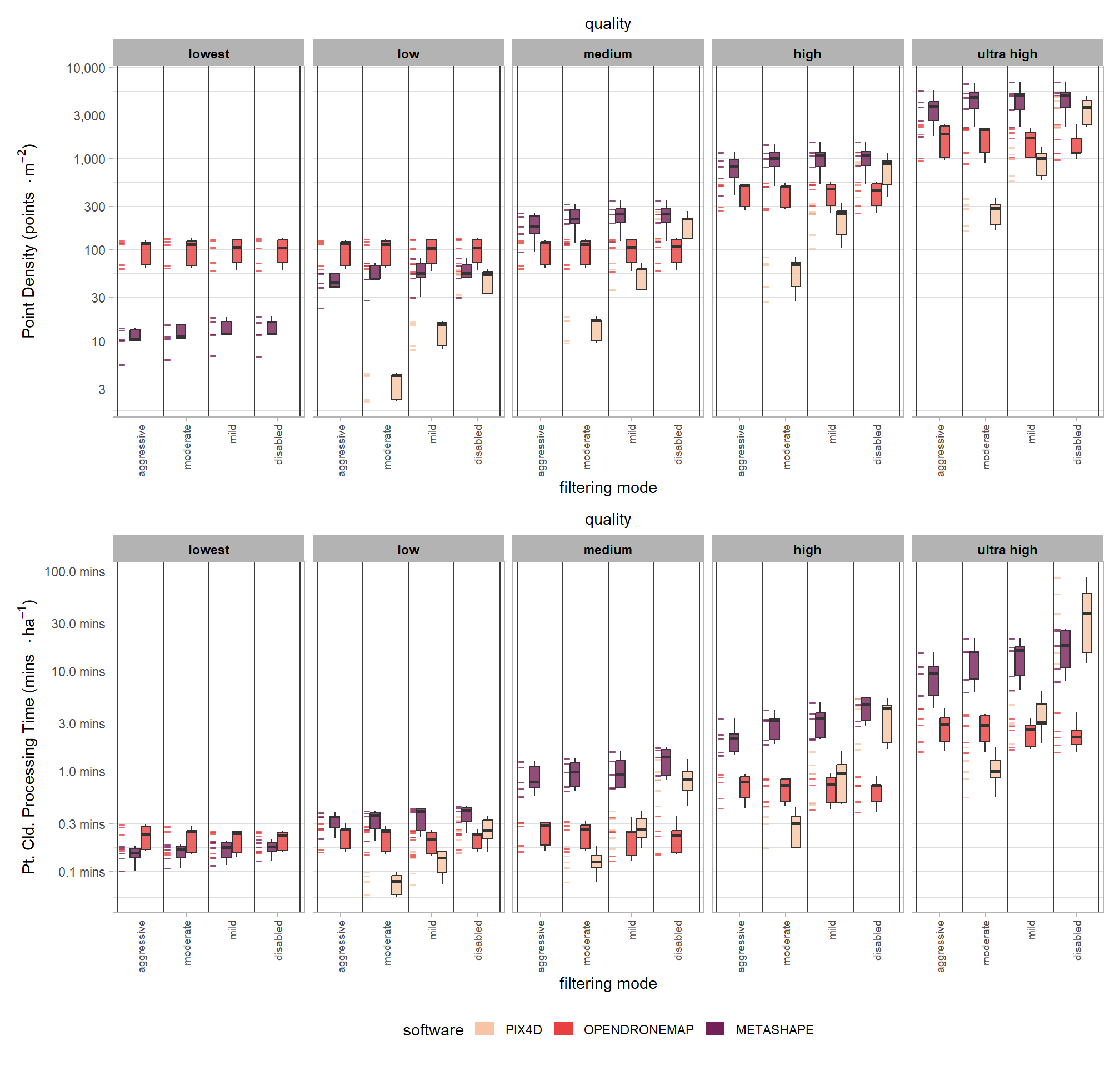
3.6.3 SfM image processing time summary
Summary of the normalized SfM image processing time normalized using Min-Max normalization as:
\[ x^{\prime}_{ij} = \frac{x_{ij}-x_{min[j]}}{x_{max[j]}-x_{min[j]}} \]
where \(i\) is the the study site observation within each software \(j\) where each software was implemented on a different computer.
ptcld_processing_data %>%
  dplyr::group_by(software, depth_maps_generation_quality, depth_maps_generation_filtering_mode) %>%
  dplyr::mutate(med = median(total_sfm_time_norm, na.rm = T)) %>%
  dplyr::ungroup() %>%
  dplyr::mutate(depth_maps_generation_quality = forcats::fct_rev(depth_maps_generation_quality)) %>%
  ggplot(mapping = aes(
    x = depth_maps_generation_filtering_mode
    , y = total_sfm_time_norm
    , fill = med
  )) +
    geom_boxplot(width = 0.7, outliers = F, fill = "slategray") +
    facet_grid(
      rows = vars(software)
      , cols = vars(depth_maps_generation_quality)
    ) +
    scale_fill_viridis_c(option = "mako", direction = -1, end = 0.9) +
    scale_y_continuous(
      limits = c(-0.02,1.02)
      , breaks = c(0, 1)
      , minor_breaks = seq(0.2,0.8,0.2)
      , labels = c("min","max")
    ) +
    labs(x = "filtering mode", y = "SfM Image Processing Time (normalized)",subtitle = "quality") +
    theme_light() +
    theme(
      legend.position = "none"
      , legend.direction  = "horizontal"
      , panel.grid.major.x = element_blank()
      , panel.grid.minor.x = element_blank()
      , panel.grid.major.y = element_line(color = "black")
      , axis.ticks.y = element_blank()
      , axis.text.x = element_text(angle = 90, vjust = 0.5, hjust = 1)
      , strip.text = element_text(color = "black", face = "bold")
      , plot.subtitle = element_text(hjust = 0.5)
    )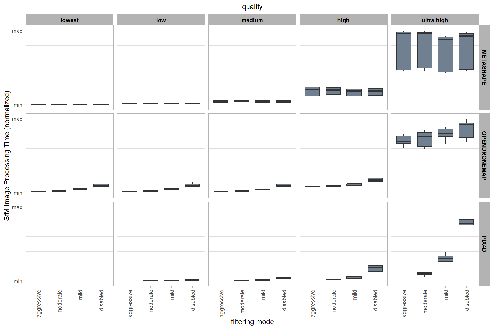
table it
table_temp =
  ptcld_processing_data %>%
  dplyr::group_by(software, depth_maps_generation_quality, depth_maps_generation_filtering_mode) %>%
  dplyr::summarise(
    dplyr::across(
      total_sfm_time_norm
      , .fns = list(mean = mean, sd = sd, min = min, max = max)
    )
    , n = dplyr::n()
  ) %>%
  dplyr::mutate(
    range = paste0(
      total_sfm_time_norm_min %>% scales::number(accuracy = 0.01)
      , "—"
      , total_sfm_time_norm_max %>% scales::number(accuracy = 0.01)
    )
    , depth_maps_generation_quality = depth_maps_generation_quality %>% forcats::fct_rev()
  ) %>%
  select(-c(n,total_sfm_time_norm_min, total_sfm_time_norm_max)) %>%
  dplyr::ungroup() %>%
  dplyr::arrange(software, depth_maps_generation_quality, depth_maps_generation_filtering_mode)

table_temp %>%
  # dplyr::select(-c(software)) %>%
  kableExtra::kbl(
    digits = 2
    , caption = "Normalized SfM Image Processing Time"
    , col.names = c(
      "software", "quality", "filtering mode"
      , "Mean"
      , "Std Dev", "Range"
    )
    , escape = F
  ) %>%
  kableExtra::kable_styling() %>%
  # kableExtra::pack_rows(index = table(forcats::fct_inorder(table_temp$software))) %>%
  kableExtra::collapse_rows(columns = 1:2, valign = "top") %>%
kableExtra::scroll_box(height = "8in")| software | quality | filtering mode | Mean | Std Dev | Range |
|---|---|---|---|---|---|
| METASHAPE | lowest | aggressive | 0.00 | 0.00 | 0.00—0.01 |
| moderate | 0.00 | 0.00 | 0.00—0.01 | ||
| mild | 0.00 | 0.00 | 0.00—0.01 | ||
| disabled | 0.00 | 0.00 | 0.00—0.01 | ||
| low | aggressive | 0.01 | 0.01 | 0.00—0.02 | |
| moderate | 0.01 | 0.01 | 0.00—0.02 | ||
| mild | 0.01 | 0.01 | 0.00—0.02 | ||
| disabled | 0.01 | 0.01 | 0.00—0.02 | ||
| medium | aggressive | 0.04 | 0.02 | 0.02—0.06 | |
| moderate | 0.04 | 0.02 | 0.02—0.06 | ||
| mild | 0.04 | 0.02 | 0.02—0.05 | ||
| disabled | 0.04 | 0.02 | 0.02—0.06 | ||
| high | aggressive | 0.18 | 0.07 | 0.10—0.24 | |
| moderate | 0.18 | 0.06 | 0.10—0.23 | ||
| mild | 0.16 | 0.06 | 0.09—0.21 | ||
| disabled | 0.17 | 0.06 | 0.09—0.22 | ||
| ultra high | aggressive | 0.77 | 0.29 | 0.45—1.00 | |
| moderate | 0.78 | 0.28 | 0.46—1.00 | ||
| mild | 0.72 | 0.26 | 0.43—0.93 | ||
| disabled | 0.76 | 0.27 | 0.45—0.99 | ||
| OPENDRONEMAP | lowest | aggressive | 0.02 | 0.00 | 0.02—0.02 |
| moderate | 0.02 | 0.01 | 0.00—0.03 | ||
| mild | 0.05 | 0.00 | 0.04—0.05 | ||
| disabled | 0.11 | 0.02 | 0.08—0.14 | ||
| low | aggressive | 0.02 | 0.00 | 0.02—0.03 | |
| moderate | 0.03 | 0.00 | 0.02—0.03 | ||
| mild | 0.05 | 0.01 | 0.04—0.06 | ||
| disabled | 0.11 | 0.03 | 0.08—0.15 | ||
| medium | aggressive | 0.02 | 0.00 | 0.02—0.02 | |
| moderate | 0.02 | 0.00 | 0.02—0.03 | ||
| mild | 0.05 | 0.00 | 0.04—0.05 | ||
| disabled | 0.11 | 0.02 | 0.09—0.14 | ||
| high | aggressive | 0.09 | 0.01 | 0.08—0.10 | |
| moderate | 0.09 | 0.01 | 0.08—0.10 | ||
| mild | 0.12 | 0.01 | 0.10—0.13 | ||
| disabled | 0.18 | 0.03 | 0.14—0.22 | ||
| ultra high | aggressive | 0.71 | 0.08 | 0.61—0.80 | |
| moderate | 0.73 | 0.11 | 0.60—0.85 | ||
| mild | 0.79 | 0.09 | 0.66—0.90 | ||
| disabled | 0.86 | 0.13 | 0.69—1.00 | ||
| PIX4D | low | moderate | 0.00 | 0.00 | 0.00—0.01 |
| mild | 0.01 | 0.00 | 0.01—0.01 | ||
| disabled | 0.01 | 0.01 | 0.01—0.02 | ||
| medium | moderate | 0.01 | 0.01 | 0.00—0.02 | |
| mild | 0.02 | 0.00 | 0.01—0.02 | ||
| disabled | 0.04 | 0.01 | 0.02—0.05 | ||
| high | moderate | 0.02 | 0.01 | 0.01—0.03 | |
| mild | 0.06 | 0.02 | 0.03—0.08 | ||
| disabled | 0.18 | 0.07 | 0.12—0.28 | ||
| ultra high | moderate | 0.10 | 0.03 | 0.05—0.12 | |
| mild | 0.29 | 0.09 | 0.15—0.39 | ||
| disabled | 0.78 | 0.17 | 0.54—1.00 |