Section 5 Field Validation

This section combines the SfM-derived tree locations with stem-mapped tree locations from field sampling.

Tinkham and Swayze (2021; p.6) describe a methodology for matching UAS detected trees with stem mapped trees identified via traditional field survey methods. Note, detected trees in the excerpt below references UAS detected trees while survey trees references field-based stem mapped trees:

Each of the detected tree outputs was matched with survey tree locations through an iterative process. Iteratively, a detected tree was selected, and all survey trees within a 3 m radius and 10% height of the detected tree were identified. If a survey tree met both the location and height precision requirements, it was considered a true positive (TP) detection, and both the survey and detected trees were removed from further matching. However, if no match was made, the detected tree was considered a commission (Co) and removed from further matching. This process was repeated until all detected trees were classified as true positive or commission, with all unmatched survey trees classified as omission (Om). Overall tree detection performance was described using the F-score metric.

The F-score incorporates true positive, commission, and omission rates to determine how well the UAS detected trees represent the field-based stem mapped trees. As a measure of predictive performance, the highest possible value of an F-score is 1.0, indicating perfect precision and recall, and the lowest possible value is 0, if either precision or recall are zero.

\[ \textrm{F-score} = 2 \times \frac{\bigl(\frac{TP}{TP+Om} \times \frac{TP}{TP+Co} \bigr)}{\bigl(\frac{TP}{TP+Om} + \frac{TP}{TP+Co} \bigr)} \]

The process to match UAS detected trees to field stem mapped trees implemented here is slightly different than the process described above. To match the data parametrization from the UAS point cloud processing workflow, only stem-mapped trees above 2 m were considered for analysis. Each UAS detected tree was matched with stem-mapped tree locations that were within a 3 m radius and 2 m height of the UAS detected tree. The matched UAS and stem-mapped tree pairs were jointly compared (rather than iteratively) to select the pair that minimized the height difference for both the stem-mapped tree and the UAS detected tree to ensure that only one UAS detected tree was selected for each stem-mapped tree. If more than one UAS detected tree had the same height difference to a stem-mapped tree, the UAS detected tree spatially nearest to the stem-mapped tree was selected as the match. These UAS detected trees with a paired stem-mapped tree after this filtering process were considered true positive (\(TP\)) detections.

To determine UAS detected tree commissions (i.e. UAS detected trees within the overstory plot for which there was no stem-mapped tree pair; \(Co\)) this analysis used the 2023-06 BHEF overstory field survey plot center and plot radius with a minimum DBH of 5 in (12.69 cm) as only trees above this size were sampled as part of the overstory survey. UAS detected trees within this radius with an estimated DBH over 5 in (12.69 cm) that did not have a matched stem-mapped tree pair were considered commissions (\(Co\)). The 2023-06 BHEF field surveys used \(\frac{1}{10}\) acre (404.686 m²) plots with a 37.24 ft (11.35 m) radius for overstory sampling and \(\frac{1}{400}\) acre (10.117 m²) plots with a 5.89 ft (1.795 m) radius for regeneration sampling. All unmatched stem-mapped survey trees were classified as omissions (\(Om\)).

5.1 Setup

Pick a DBH to use for the validation. For this project, the UAS point cloud processing script utilized the random forest model to estimate missing DBH values using training values extracted from the point cloud using the TreeLS package. The script below adds two linear model estimates of DBH based on the training data: 1) a linear model with an intercept (dbh_cm ~ 1 + tree_height_m); and 2) a linear model with no intercept (dbh_cm ~ 0 + tree_height_m).

The options for picking a DBH to use are:

1. “rf” for random forest estimate
2. “lin” for linear model with an intercept (dbh_cm ~ 1 + tree_height_m) estimate
3. “lin_noint” for linear model with no intercept (dbh_cm ~ 0 + tree_height_m) estimate
4. “regional” for regional estimate based on regional FIA data using the USFS TreeMap data

# Pick a DBH to use for the validation
# my_dbh_estimate = "lin"
my_dbh_estimate = "regional"

Load field validation plot data and update the ptcld_processing_data created in this section by adding a processing_id which we’ll use to process the files for validation.

# list of study sites with completed uas data
study_site_list = ptcld_processing_data$study_site %>% unique() %>% toupper()

# list of field validation data
validation_data =
  list.files(
    "../data/field_validation"
    , pattern = "\\.gpkg$", full.names = T
  ) %>% 
  normalizePath() %>% 
  dplyr::as_tibble() %>% 
  dplyr::rename(validation_file_full_path=1) %>% 
  dplyr::mutate(
    study_site = validation_file_full_path %>% 
      toupper() %>% 
      stringr::str_extract(pattern = paste(study_site_list, collapse = "|"))
  ) %>% 
  dplyr::filter(study_site %in% study_site_list) %>% 
  dplyr::group_by(study_site) %>% 
  dplyr::filter(dplyr::row_number() == 1) %>% 
  dplyr::ungroup()

# what about the field plot boundary?
validation_plots = sf::st_read("../data/field_validation/Field_Data_Boundary.shp") %>% 
  dplyr::rename_with(tolower) %>% 
  dplyr::mutate(
    study_site = site %>% 
      toupper() %>% 
      stringr::str_extract(pattern = paste(study_site_list, collapse = "|"))
  ) %>% 
  dplyr::filter(study_site %in% study_site_list) %>% 
  dplyr::group_by(study_site) %>% 
  dplyr::filter(dplyr::row_number() == 1) %>% 
  dplyr::ungroup() %>% 
  dplyr::mutate(
    area_ha = sf::st_area(.) %>% as.numeric() %>% `/`(10000)
    , area_acres = area_ha*2.471
  )

## Reading layer `Field_Data_Boundary' from data source 
##   `C:\Data\usfs\metashape_testing\data\field_validation\Field_Data_Boundary.shp' 
##   using driver `ESRI Shapefile'
## Simple feature collection with 5 features and 4 fields
## Geometry type: POLYGON
## Dimension:     XY
## Bounding box:  xmin: -157287.6 ymin: 4068511 xmax: 608828.5 ymax: 4892131
## Projected CRS: WGS 84 / UTM zone 13N

# where is the uas processed data?
ptcld_processing_data =
  ptcld_processing_data %>% 
  dplyr::mutate(
    processed_data_dir = dirname(tracking_file_full_path)
    , processing_id = dplyr::row_number()
  )

where are these validation plots and what do they look like?

# what?
validation_plots %>% dplyr::glimpse()

## Rows: 5
## Columns: 8
## $ id         <dbl> NA, NA, NA, NA, NA
## $ site       <chr> "WA85_02", "SQ09_02", "N1", "Kaibab_Low", "Kaibab_High"
## $ acres      <dbl> 2.476617, 2.476617, 3.911949, 5.059504, 4.264751
## $ hectares   <dbl> 1.002679, 1.002679, 1.583785, 2.048382, 1.726620
## $ geometry   <POLYGON [m]> POLYGON ((608678.6 4892131,..., POLYGON ((608720.2 4889252,…
## $ study_site <chr> "WA85_02", "SQ09_02", "N1", "KAIBAB_LOW", "KAIBAB_HIGH"
## $ area_ha    <dbl> 1.002168, 1.002168, 1.582522, 2.068603, 1.743671
## $ area_acres <dbl> 2.476358, 2.476358, 3.910412, 5.111518, 4.308611

# where?
mapview::mapviewOptions(basemaps = c("OpenStreetMap","Esri.WorldImagery"))
validation_plots %>% 
  sf::st_buffer(2000) %>% # because they are small
  mapview::mapview(col.regions = "blue", layer.name = "plot", alpha.regions = 0.7)

create a function to calculate the basal area of a tree in m² from DBH measured in cm

calc_ba_m2_from_dbh_cm = function(dbh_cm){
  return(
    pi * dbh_cm^2 / (4*10000)
  )
}

5.2 Data Load Functions

field validation data

# function to read field data once per site
read_field_data <- function(my_study_site) {
  d = sf::st_read(
    validation_data %>% 
      dplyr::filter(study_site == my_study_site) %>% 
      dplyr::pull(validation_file_full_path)
    ) %>% 
    dplyr::mutate(
      study_site = my_study_site
    ) %>% 
    dplyr::rename_with(tolower) %>% 
    dplyr::rename(
      field_dbh_cm = dbh_cm
      , field_tree_height_m = ht_m
    ) %>% 
    sf::st_set_geometry("geometry") %>% 
    dplyr::filter(
      !is.na(field_dbh_cm)
      & !is.na(field_tree_height_m)
      & sf::st_is_valid(geometry)
      # only keep trees that are above height threshold used for uas processing
      & field_tree_height_m >= min(ptcld_processing_data$sttng_minimum_tree_height_m)
      # & field_dbh_cm >= min_tree_dbh_cm # if know min field dbh for field sampling
    )
  # keep only trees within sampling plot
  d %>% 
    sf::st_intersection(
      validation_plots %>% 
        dplyr::filter(study_site == my_study_site) %>% 
        dplyr::mutate(intersected_with_plot_geom = T) %>% 
        dplyr::select(intersected_with_plot_geom) %>% 
        sf::st_transform(sf::st_crs(d))
    ) %>% 
    dplyr::mutate(
      field_tree_id = dplyr::row_number()
      , tree_utm_x = sf::st_coordinates(geometry)[,1] #lon
      , tree_utm_y = sf::st_coordinates(geometry)[,2] #lat
      # basal area
      , basal_area_m2 = calc_ba_m2_from_dbh_cm(field_dbh_cm)
    ) %>% 
    dplyr::relocate(field_tree_id)
    
}

5.2.1 Summary of field validation plot data

table_temp = validation_plots %>% 
  dplyr::pull(study_site) %>% 
  purrr::map(function(x){
    read_field_data(x) %>% 
      sf::st_drop_geometry() %>% 
      dplyr::select(study_site,field_dbh_cm,field_tree_height_m,basal_area_m2)
  }) %>% 
  dplyr::bind_rows() %>% 
  dplyr::group_by(study_site) %>% 
  dplyr::summarise(
    dplyr::across(
      tidyselect::starts_with("field_")
      , .fns = list(mean = mean, sd = sd)
    )
    , n_trees = dplyr::n()
    , basal_area_m2 = sum(basal_area_m2)
  ) %>% 
  # add area
  dplyr::inner_join(
    validation_plots %>% dplyr::select(study_site, area_ha) %>% sf::st_drop_geometry()
    , by = "study_site"
  ) %>% 
  dplyr::mutate(
    ht = paste0(
      field_tree_height_m_mean %>% 
        round(1) %>% 
        scales::comma(accuracy = 0.1)
      , "<br>("
      , field_tree_height_m_sd %>% 
          round(1) %>% 
          scales::comma(accuracy = 0.1)
      , ")"
    )
    , dbh = paste0(
      field_dbh_cm_mean %>% round(1) %>% scales::comma(accuracy = 0.1)
      , "<br>("
      , field_dbh_cm_sd %>% round(1) %>% scales::comma(accuracy = 0.1)
      , ")"
    )
    , trees_ha = n_trees/area_ha
    , basal_area_m2_per_ha = basal_area_m2/area_ha
    , area_ha = area_ha %>% round(1) %>% scales::comma(accuracy = 0.1)
  ) %>% 
  dplyr::select(
    study_site, area_ha, trees_ha, basal_area_m2_per_ha, ht, dbh
  )

table_temp %>% 
  kableExtra::kbl(
    escape = F
    , digits = 1
    , col.names = c(
      ""
      , "Hectares"
      , "Trees<br>ha<sup>-1</sup>"
      , "Basal Area<br>m<sup>2</sup> ha<sup>-1</sup>"
      , "Height (m)", "DBH (cm)"
    )
  ) %>% 
  kableExtra::kable_styling()

	Hectares	Trees ha-1	Basal Area m2 ha-1	Height (m)	DBH (cm)
KAIBAB_HIGH	1.7	574.1	39.6	12.8 (7.2)	24.0 (17.4)
KAIBAB_LOW	2.1	246.5	22.5	12.5 (8.6)	27.3 (20.5)
N1	1.6	639.5	24.8	8.5 (7.3)	15.4 (16.0)
SQ09_02	1.0	308.3	11.2	11.1 (4.8)	19.7 (8.8)
WA85_02	1.0	171.6	14.9	15.7 (6.0)	30.7 (12.8)

5.2.2 Load UAS data function

# function finds uas tree list
# reads it
# estimates linear model if not already used for DBH
read_uas_data = function(my_processing_id, my_crs = NULL, use_this_dbh = my_dbh_estimate) {
  # where is this file?
  fnm = ptcld_processing_data %>% 
    dplyr::filter(
      processing_id == my_processing_id
    ) %>% 
    dplyr::mutate(
      fnm = paste0(
        processed_data_dir
        , "/"
        , file_name
        , "_final_detected_tree_tops.gpkg"
      )
    ) %>% 
    dplyr::pull(fnm)
  
  if(file.exists(fnm)){
    # read it
    dta = sf::st_read(fnm) %>% 
      dplyr::mutate(
        processing_id = my_processing_id
      ) %>% 
      dplyr::rename_with(tolower) %>% 
      sf::st_set_geometry("geometry")
    
    # transform
    if(is.null(my_crs)){
      tcrs = sf::st_crs(dta)
    }else{tcrs = my_crs}
    
    dta = dta %>% 
      sf::st_transform(tcrs)
    
    #################
    # estimate linear model if not already used for DBH
    #################
    if(
      # is there sufficient training data?
      dta %>% 
        dplyr::filter(is_training_data == T) %>% 
        nrow() > 10 & 
      # was rf model used?
      ptcld_processing_data %>% 
        dplyr::filter(processing_id == my_processing_id) %>% 
        dplyr::pull(sttng_local_dbh_model) %>% 
        tolower() == "rf"
    ){
        # Gamma distribution for strictly positive response variable dbh
          # !!!! fit with intercept 
        stem_prediction_model = brms::brm(
          formula = dbh_cm ~ 1 + tree_height_m
          , data = dta %>%
              dplyr::filter(is_training_data==T) %>% 
              dplyr::select(dbh_cm, tree_height_m)
          , family = brms::brmsfamily("Gamma", link = "log")
          , prior = c(prior(gamma(0.01, 0.01), class = shape))
          , iter = 4000, warmup = 2000, chains = 4
          , cores = lasR::half_cores()
          , file = ptcld_processing_data %>%
              dplyr::filter(processing_id == my_processing_id) %>%
              dplyr::mutate(
                fff = paste0(
                  processed_data_dir
                  , "/"
                  , file_name
                  , "_local_dbh_height_model"
                )
              ) %>%
              dplyr::pull(fff)
          # , file_refit = "on_change"
        )
        
        # Gamma distribution for strictly positive response variable dbh
          # !!!! fit with NO intercept 
        stem_prediction_noint_model = brms::brm(
          formula = dbh_cm ~ 0 + tree_height_m
          , data = dta %>%
              dplyr::filter(is_training_data==T) %>% 
              dplyr::select(dbh_cm, tree_height_m)
          , family = brms::brmsfamily("Gamma", link = "log")
          , prior = c(prior(gamma(0.01, 0.01), class = shape))
          , iter = 4000, warmup = 2000, chains = 4
          , cores = lasR::half_cores()
          , file = ptcld_processing_data %>%
              dplyr::filter(processing_id == my_processing_id) %>%
              dplyr::mutate(
                fff = paste0(
                  processed_data_dir
                  , "/"
                  , file_name
                  , "_local_dbh_height_noint_model"
                )
              ) %>%
              dplyr::pull(fff)
          # , file_refit = "on_change"
        )
      #################
      # prediction data
      #################
        pred_temp = predict(stem_prediction_model, dta) %>% 
          dplyr::as_tibble() %>% 
          dplyr::pull(1)
        
        pred_noint_temp = predict(stem_prediction_noint_model, dta) %>% 
          dplyr::as_tibble() %>% 
          dplyr::pull(1)
        
        # add to data
        dta = dta %>% 
          dplyr::mutate(
            rf_dbh_cm = dbh_cm
            , pred_dbh_cm = pred_temp
            , pred_noint_dbh_cm = pred_noint_temp
            , lin_dbh_cm = ifelse(is_training_data==T, dbh_cm, pred_dbh_cm)
            , lin_noint_dbh_cm = ifelse(is_training_data==T, dbh_cm, pred_noint_dbh_cm)
          ) %>% 
          dplyr::select(-c(pred_dbh_cm,pred_noint_dbh_cm))
    }else if(# is there sufficient training data?
      dta %>% 
        dplyr::filter(is_training_data == T) %>% 
        nrow() <= 10
    ){
      # the regional model was used which would result in the same est for rf and lin
      dta = dta %>% 
        dplyr::mutate(
          rf_dbh_cm = dbh_cm
          , lin_dbh_cm = dbh_cm
          , lin_noint_dbh_cm = dbh_cm
        )
    }else{
      # linear model was already used and no rf pred
      # could update this to estimate rf model if missing...#nextyear
      dta = dta %>% 
        dplyr::mutate(
          rf_dbh_cm = as.numeric(NA)
          , lin_dbh_cm = dbh_cm
          , lin_noint_dbh_cm = as.numeric(NA)
        )
    }
    # return with dbh updated
    return(
      dta %>% 
        dplyr::mutate(
          dbh_cm = dplyr::case_when(
          # update dbh to selected
          tolower(use_this_dbh) == "rf" & !is.na(rf_dbh_cm) ~ rf_dbh_cm
          , tolower(use_this_dbh) == "lin" & !is.na(lin_dbh_cm) ~ lin_dbh_cm
          , tolower(use_this_dbh) == "lin_noint" & !is.na(lin_noint_dbh_cm) ~ lin_noint_dbh_cm
          , tolower(use_this_dbh) == "regional" & !is.na(reg_est_dbh_cm) ~ reg_est_dbh_cm
          , T ~ reg_est_dbh_cm
        )) %>% 
        dplyr::mutate(
          basal_area_m2 = calc_ba_m2_from_dbh_cm(dbh_cm)
          , basal_area_ft2 = basal_area_m2 * 10.764
        )
        
    )
  }else{stop("could not find file: ", fnm)}
}

5.3 Validation Data Functions

5.3.1 True Positive Identification

The UAS detected and stem-mapped tree pairs identified in this filtering process (detailed above) were considered true positive (\(TP\)) detections.

## BUFFER THE UAS TREES AND SPATIALLY MATCH FIELD TREES BASED ON THAT BUFFER
true_positive_trees_fn = function(uas_data, field_data, max_dist_m = 3, max_height_error_m = 2){
  ## get FIELD trees within radius OF UAS TREES
    potential_tree_pairs_temp = uas_data %>% 
      dplyr::select(treeid, tree_height_m) %>% 
      # buffer point
      sf::st_buffer(max_dist_m) %>% 
      # spatial join with all FIELD tree points
      sf::st_join(
        field_data %>% 
          dplyr::select(
            field_tree_id, field_tree_height_m
            , tree_utm_x, tree_utm_y
          )
        , join = sf::st_intersects
        , left = F # performs inner join to only keep uas trees with a match
      ) %>% 
      # calculate height difference
      dplyr::mutate(
        height_diff_m = abs(tree_height_m-field_tree_height_m)
        , height_diff_pct = height_diff_m/field_tree_height_m
      ) %>% 
      # removes tree pairs that are outside of the allowable error
      # dplyr::filter(height_diff_pct <= max_height_error_pct) %>% 
      dplyr::filter(height_diff_m <= max_height_error_m) %>% 
      dplyr::select(-c(height_diff_m)) %>% 
      dplyr::relocate(treeid, field_tree_id)
  
  ## apply pair selection criteria if there are potential tree pairs
    if(nrow(potential_tree_pairs_temp)>0){
      ## calculate row by row distances and height differences
        potential_tree_pairs_temp = potential_tree_pairs_temp %>% 
          # this is the position of the uas tree
          sf::st_centroid() %>% 
          sf::st_set_geometry("geom1") %>% 
          dplyr::bind_cols(
            potential_tree_pairs_temp %>% 
              sf::st_drop_geometry() %>% 
              dplyr::select("tree_utm_x", "tree_utm_y") %>% 
              # this is the position of the field tree
              sf::st_as_sf(
                coords = c("tree_utm_x", "tree_utm_y"), crs = sf::st_crs(uas_data)
              ) %>% 
              sf::st_set_geometry("geom2")
          ) %>% 
          dplyr::mutate(
            distance_m = sf::st_distance(geom1, geom2, by_element = T) %>% as.numeric()
          ) %>% 
          sf::st_drop_geometry() %>% 
          dplyr::select(-c(tree_utm_x, tree_utm_y, geom2))
      
      ## define function to select the best tree pair
        select_best_tree_pair_fn <- function(df) {
         df %>% 
          dplyr::group_by(field_tree_id) %>% 
          dplyr::arrange(field_tree_id, height_diff_pct, distance_m, desc(tree_height_m), treeid) %>% 
          dplyr::mutate(
            # at the field tree level...the number of uas trees
            n_uas_trees = dplyr::n()
            # at the field tree level...
              # the closest uas tree in height tie breaker distance, uas_tree_height_m, id
            , rank_within_field_tree = dplyr::row_number()
          ) %>% 
          dplyr::group_by(treeid) %>% 
          dplyr::arrange(treeid, height_diff_pct, distance_m, desc(field_tree_height_m), field_tree_id) %>% 
          dplyr::mutate(
            # at the uas tree level...the number of field trees
            n_field_trees = dplyr::n()
            # at the field tree level...
              # the closest field tree in height tie breaker distance, uas_tree_height_m, id
            , rank_within_uas_tree = dplyr::row_number()
          ) %>% 
          dplyr::ungroup() %>% 
          # select the uas-field tree pair with the minimum height difference
          dplyr::filter(
            rank_within_field_tree == 1
            & rank_within_uas_tree == 1
          ) %>% 
          # remove columns
          dplyr::select(
            -c(tidyselect::starts_with("rank_"), tidyselect::starts_with("n_"))
          )
        }
      
      ## first filter for tree pairs
        true_positive_trees = select_best_tree_pair_fn(potential_tree_pairs_temp)
      
      ##remove matches from potential tree pairs 
        potential_tree_pairs_temp = potential_tree_pairs_temp %>% 
          dplyr::filter(
            !(treeid %in% true_positive_trees$treeid)
            & !(field_tree_id %in% true_positive_trees$field_tree_id)
          )
        
      ## keep filtering for best pair until no unique pairs remain
        while(nrow(potential_tree_pairs_temp)>0) {
          # keep filtering for best pair until no unique pairs remain
          true_positive_trees = true_positive_trees %>% 
            dplyr::bind_rows(
              select_best_tree_pair_fn(potential_tree_pairs_temp)
            )
          #remove matches from potential tree pairs 
          potential_tree_pairs_temp = potential_tree_pairs_temp %>% 
            dplyr::filter(
              !(treeid %in% true_positive_trees$treeid)
              & !(field_tree_id %in% true_positive_trees$field_tree_id)
            )
        }
      ## rename columns and flag
        true_positive_trees = true_positive_trees %>% 
          dplyr::rename(
            uas_tree_height_m = tree_height_m
            , uas_tree_id = treeid
            , field_uas_distance_m = distance_m
          ) %>% 
          dplyr::mutate(
            field_uas_group = "true positive"
          ) 
    }else{ # if there are spatially matched trees
      true_positive_trees = dplyr::tibble(
        uas_tree_id = as.character(NA)
        , field_tree_id = as.character(NA)
        , uas_tree_height_m = as.numeric(NA)
        , field_tree_height_m = as.numeric(NA)
        , height_diff_pct = as.numeric(NA)
        , field_uas_distance_m = as.numeric(NA)
        , field_uas_group = as.character(NA)
      )
    }
  # return
    return(true_positive_trees)
}

5.3.2 Combine with Commission and Omission

To determine UAS detected tree commissions (i.e. UAS detected trees within the overstory plot for which there was no stem-mapped tree pair; \(Co\)) this analysis used the 2023-06 BHEF overstory field survey plot center and plot radius of 11.35 m. UAS detected trees within this radius with an estimated DBH over 5 in (12.69 cm) that did not have a matched stem-mapped tree pair were considered commissions (\(Co\)).

Omissions (\(Om\)) are stem-mapped trees without a UAS detected tree match.

field_uas_comparison_fn = function(uas_data, field_data, true_positive_trees, plot_data, overstory_ht_m = 7){
  field_uas_comparison = dplyr::bind_rows(
    ## true positive
      true_positive_trees %>% 
         dplyr::mutate(field_tree_id = as.numeric(field_tree_id))
    ## omission
      , field_data %>% 
        sf::st_drop_geometry() %>% 
        dplyr::select(
          field_tree_id, field_tree_height_m
        ) %>% 
        dplyr::anti_join(
          true_positive_trees %>% 
            dplyr::mutate(field_tree_id = as.numeric(field_tree_id))
          , by = dplyr::join_by(field_tree_id)
        ) %>% 
        dplyr::mutate(
          field_uas_group = "omission"
        )
    ## commission
      , plot_data %>% 
        sf::st_transform(sf::st_crs(uas_data)) %>% 
        dplyr::select(study_site) %>% 
        # join with uas tree points
        sf::st_join(
          uas_data %>% 
            dplyr::filter(
              !treeid %in% true_positive_trees$uas_tree_id
            ) %>% 
            dplyr::select(treeid) %>% 
            dplyr::rename(uas_tree_id=treeid)
          , join = sf::st_intersects
          , left = F # performs inner join to only keep uas trees and plots with a match
        ) %>% 
        dplyr::select(-c(study_site)) %>% 
        sf::st_drop_geometry() %>% 
        dplyr::mutate(
          field_uas_group = "commission"
        )
  ) %>% 
  dplyr::filter(!is.na(field_uas_group) & field_uas_group!="") %>% 
    # attach uas data
    dplyr::left_join(
      uas_data %>%
        sf::st_set_geometry("geometry") %>% 
        dplyr::mutate(
          uas_tree_utm_x = sf::st_coordinates(geometry)[,1] #lon
          , uas_tree_utm_y = sf::st_coordinates(geometry)[,2] #lat
        ) %>% 
        sf::st_drop_geometry() %>% 
        dplyr::select(treeid, tree_height_m, dbh_cm, basal_area_m2, uas_tree_utm_x, uas_tree_utm_y) %>% 
        dplyr::rename(
          uas_tree_id = treeid
          , uas_tree_height_m = tree_height_m
          , uas_dbh_cm = dbh_cm
          , uas_basal_area_m2 = basal_area_m2
        )
      , by = dplyr::join_by(uas_tree_id)
    ) %>% 
    # attach field data
    dplyr::left_join(
      field_data %>% 
        sf::st_drop_geometry() %>% 
        dplyr::select(
          field_tree_id, field_tree_height_m, field_dbh_cm, basal_area_m2
          , tree_utm_x, tree_utm_y
        ) %>% 
        dplyr::rename(
          field_basal_area_m2 = basal_area_m2
          , field_tree_utm_x = tree_utm_x
          , field_tree_utm_y = tree_utm_y
        )
      , by = dplyr::join_by(field_tree_id)
    ) %>% 
    # update data
    dplyr::mutate(
      uas_tree_height_m = uas_tree_height_m.y
      , field_tree_height_m = field_tree_height_m.y
      , field_uas_group = factor(
        field_uas_group
        , ordered = T
        , levels = c(
          "true positive"
          , "commission"
          , "omission"
        )
      ) %>% forcats::fct_rev()
      , dbh_diff_cm = uas_dbh_cm - field_dbh_cm
      , tree_height_diff_m = uas_tree_height_m - field_tree_height_m
      , dbh_diff_pct = dbh_diff_cm/field_dbh_cm
      , height_diff_pct = tree_height_diff_m/field_tree_height_m
      , abs_dbh_diff_pct = abs(dbh_diff_pct)
      , abs_height_diff_pct = abs(height_diff_pct)
      # determine overstory/understory
      , overstory_understory_grp = dplyr::case_when(
        dplyr::coalesce(field_tree_height_m, uas_tree_height_m) >= overstory_ht_m ~ "overstory"
        , dplyr::coalesce(field_tree_height_m, uas_tree_height_m) < overstory_ht_m ~ "understory"
        , T ~ "error"
      ) %>% factor()
      # attach identifying data
      , study_site = uas_data$study_site[1]
      , file_name = uas_data$file_name[1]
      , software = uas_data$software[1]
      , overstory_ht_m = overstory_ht_m
    ) %>% 
    dplyr::relocate(field_uas_group) %>% 
    dplyr::select(-c(tidyselect::ends_with(".x"), tidyselect::ends_with(".y")))
    # # convert to imperial units
    # calc_imperial_units_fn()
  # return
  return(field_uas_comparison)
}

5.3.3 Full validation function

function to write comparison data and return aggregate metrics when passed a ptcld_processing_data$processing_id

function returns:

1. write full validation tree list to disk
2. update ptcld_processing_data with metrics for testing:

• f-score
• height comparison metrics (mae, mape, smape, mse, rmse)
• dbh comparison metrics (mae, mape, smape, mse, rmse)
• path to full validation tree list written to disk

#####################################################
# function to map over each file for a particular study site
#####################################################
  # function for a file name identified by processing_id in ptcld_processing_data
  validate_file_fn = function(p_id, fld_dta, plt_dta){
    # tree list file name
      tl_fnm = paste0(
          ptcld_processing_data %>% 
            dplyr::filter(processing_id == p_id) %>% 
            dplyr::pull(processed_data_dir)
          , "/"
          , ptcld_processing_data %>% 
            dplyr::filter(processing_id == p_id) %>% 
            dplyr::pull(file_name)
          , "_field_uas_comparison_data.csv"
        )
    # brms model
      brms_fnm = paste0(
          ptcld_processing_data %>% 
            dplyr::filter(processing_id == p_id) %>% 
            dplyr::pull(processed_data_dir)
          , "/"
          , ptcld_processing_data %>% 
            dplyr::filter(processing_id == p_id) %>% 
            dplyr::pull(file_name)
          , "_local_dbh_height_model.rds"
        )
    # brms model noint
      brms_noint_fnm = paste0(
          ptcld_processing_data %>% 
            dplyr::filter(processing_id == p_id) %>% 
            dplyr::pull(processed_data_dir)
          , "/"
          , ptcld_processing_data %>% 
            dplyr::filter(processing_id == p_id) %>% 
            dplyr::pull(file_name)
          , "_local_dbh_height_noint_model.rds"
        )
    # check it
    if(file.exists(tl_fnm) & file.exists(brms_fnm) & file.exists(brms_noint_fnm)){
      # read it
      field_uas_comparison = readr::read_csv(tl_fnm)
    }else{
      # uas_data
        u_dta = read_uas_data(
          my_processing_id = p_id
          , my_crs = sf::st_crs(fld_dta)
        )
      # true positives
        tp_trees = true_positive_trees_fn(uas_data = u_dta, field_data = fld_dta)
      # field uas comparison
        field_uas_comparison = field_uas_comparison_fn(
            uas_data = u_dta
            , field_data = fld_dta
            , true_positive_trees = tp_trees
            , plot_data = plt_dta
          ) %>% 
          # attach id information
          dplyr::bind_cols(
            ptcld_processing_data %>% 
              dplyr::filter(processing_id == p_id) %>% 
              dplyr::select(
                processing_id, study_site, file_name, software
                , depth_maps_generation_quality
                , depth_maps_generation_filtering_mode
                , processing_attribute3
                , processed_data_dir
              )
          )
        # write it
        write.csv(
          field_uas_comparison
          , tl_fnm
          , row.names = F
        )
    }
    ############################################
    # aggregate field_uas_comparison for return
    ############################################
      # get plot area from plot data
      plot_area_ha = plt_dta$area_ha[1]
      # this is the return data which has lots of columns
      return_dta =
        ptcld_processing_data %>% 
        dplyr::filter(processing_id == p_id) %>%
        ############################################
        # overall statistics
        ############################################
        # attach f score
        dplyr::bind_cols(
          # blank data in case missing
          dplyr::tibble(field_uas_group = c("tp", "co", "om")) %>% 
          dplyr::left_join(
            field_uas_comparison %>% 
              dplyr::count(field_uas_group) %>% 
              dplyr::mutate(field_uas_group = dplyr::case_when(
                field_uas_group == "true positive" ~ "tp"
                , field_uas_group == "commission" ~ "co"
                , field_uas_group == "omission" ~ "om"
              ))
            , by = dplyr::join_by(field_uas_group)
          ) %>% 
          dplyr::mutate(n = ifelse(is.na(n),0,n)) %>% 
            tidyr::pivot_wider(
              names_from = field_uas_group
              , values_from = n
              , values_fill = 0
            ) %>% 
            dplyr::mutate(
              f_score = dplyr::coalesce(
                2 * ( (tp/(tp+om)) * (tp/(tp+co)) ) / ( (tp/(tp+om)) + (tp/(tp+co)) )
                , 0
              )
            ) %>% 
            dplyr::rename(
              true_positive_n_trees = tp
              , commission_n_trees = co
              , omission_n_trees = om
            ) %>% 
            dplyr::ungroup()
        ) %>% 
        # attach summary error metrics
        dplyr::bind_cols(
          field_uas_comparison %>% 
            dplyr::filter(field_uas_group=="true positive") %>% 
            dplyr::ungroup() %>% 
            # thx Metrics pkg!!
            dplyr::summarise(
              # tree_height_m
              tree_height_m_me = mean(uas_tree_height_m-field_tree_height_m, na.rm = T)
              , tree_height_m_mpe = mean((uas_tree_height_m-field_tree_height_m)/field_tree_height_m, na.rm = T)
              , tree_height_m_mae = Metrics::mae(field_tree_height_m, uas_tree_height_m)
              , tree_height_m_mape = Metrics::mape(field_tree_height_m, uas_tree_height_m)
              , tree_height_m_smape = Metrics::smape(field_tree_height_m, uas_tree_height_m)
              , tree_height_m_mse = Metrics::mse(field_tree_height_m, uas_tree_height_m)
              , tree_height_m_rmse = Metrics::rmse(field_tree_height_m, uas_tree_height_m)
              # dbh_cm
              , dbh_cm_me = mean(uas_dbh_cm-field_dbh_cm, na.rm = T)
              , dbh_cm_mpe = mean((uas_dbh_cm-field_dbh_cm)/field_dbh_cm, na.rm = T)
              , dbh_cm_mae = Metrics::mae(field_dbh_cm, uas_dbh_cm)
              , dbh_cm_mape = Metrics::mape(field_dbh_cm, uas_dbh_cm)
              , dbh_cm_smape = Metrics::smape(field_dbh_cm, uas_dbh_cm)
              , dbh_cm_mse = Metrics::mse(field_dbh_cm, uas_dbh_cm)
              , dbh_cm_rmse = Metrics::rmse(field_dbh_cm, uas_dbh_cm)
            )
        ) %>% 
        # attach basal area
        dplyr::bind_cols(
          field_uas_comparison %>% 
            dplyr::ungroup() %>% 
            dplyr::summarise(
              uas_basal_area_m2 = sum(uas_basal_area_m2, na.rm = T)
              , field_basal_area_m2 = sum(field_basal_area_m2, na.rm = T)
            ) %>% 
            # ba/ha and error
            dplyr::mutate(
              uas_basal_area_m2_per_ha = uas_basal_area_m2/plot_area_ha
              , field_basal_area_m2_per_ha = field_basal_area_m2/plot_area_ha
              # error
              , basal_area_m2_error = uas_basal_area_m2-field_basal_area_m2
              , basal_area_m2_per_ha_error = uas_basal_area_m2_per_ha-field_basal_area_m2_per_ha
              , basal_area_pct_error = (uas_basal_area_m2-field_basal_area_m2)/field_basal_area_m2
              , basal_area_abs_pct_error = abs(basal_area_pct_error)
            )
        ) %>% 
        ############################################
        # overstory/understory statistics
        ############################################
        # attach f score
        dplyr::bind_cols(
          # blank data in case missing
          tidyr::crossing(
            field_uas_group = c("tp", "co", "om")
            , overstory_understory_grp = c("overstory", "understory")
          ) %>% 
          dplyr::left_join(
            field_uas_comparison %>% 
              dplyr::count(field_uas_group, overstory_understory_grp) %>% 
              dplyr::mutate(field_uas_group = dplyr::case_when(
                field_uas_group == "true positive" ~ "tp"
                , field_uas_group == "commission" ~ "co"
                , field_uas_group == "omission" ~ "om"
              ))
            , by = dplyr::join_by(field_uas_group, overstory_understory_grp)
          ) %>% 
          dplyr::mutate(n = ifelse(is.na(n),0,n)) %>% 
            tidyr::pivot_wider(
              names_from = field_uas_group
              , values_from = n
              , values_fill = 0
            ) %>% 
            dplyr::mutate(
              f_score = dplyr::coalesce(
                2 * ( (tp/(tp+om)) * (tp/(tp+co)) ) / ( (tp/(tp+om)) + (tp/(tp+co)) )
                , 0
              )
            ) %>% 
            dplyr::rename(
              true_positive_n_trees = tp
              , commission_n_trees = co
              , omission_n_trees = om
            ) %>% 
            dplyr::ungroup() %>% 
            tidyr::pivot_wider(
              names_from = overstory_understory_grp
              , values_from = -c(overstory_understory_grp)
              , values_fill = 0
              , names_glue = "{overstory_understory_grp}_{.value}"
            )
        ) %>% 
        # attach summary error metrics
        dplyr::bind_cols(
          tidyr::crossing(
              field_uas_group = c("true positive")
              , overstory_understory_grp = c("overstory","understory")
            ) %>% 
          dplyr::left_join(
              field_uas_comparison %>%
                dplyr::mutate(overstory_understory_grp=as.character(overstory_understory_grp))
              , by = dplyr::join_by("field_uas_group", "overstory_understory_grp")
            ) %>% 
            dplyr::group_by(overstory_understory_grp) %>% 
            # thx Metrics pkg!!
            dplyr::summarise(
              # tree_height_m
              tree_height_m_me = mean(uas_tree_height_m-field_tree_height_m, na.rm = T)
              , tree_height_m_mpe = mean((uas_tree_height_m-field_tree_height_m)/field_tree_height_m, na.rm = T)
              , tree_height_m_mae = Metrics::mae(field_tree_height_m, uas_tree_height_m)
              , tree_height_m_mape = Metrics::mape(field_tree_height_m, uas_tree_height_m)
              , tree_height_m_smape = Metrics::smape(field_tree_height_m, uas_tree_height_m)
              , tree_height_m_mse = Metrics::mse(field_tree_height_m, uas_tree_height_m)
              , tree_height_m_rmse = Metrics::rmse(field_tree_height_m, uas_tree_height_m)
              # dbh_cm
              , dbh_cm_me = mean(uas_dbh_cm-field_dbh_cm, na.rm = T)
              , dbh_cm_mpe = mean((uas_dbh_cm-field_dbh_cm)/field_dbh_cm, na.rm = T)
              , dbh_cm_mae = Metrics::mae(field_dbh_cm, uas_dbh_cm)
              , dbh_cm_mape = Metrics::mape(field_dbh_cm, uas_dbh_cm)
              , dbh_cm_smape = Metrics::smape(field_dbh_cm, uas_dbh_cm)
              , dbh_cm_mse = Metrics::mse(field_dbh_cm, uas_dbh_cm)
              , dbh_cm_rmse = Metrics::rmse(field_dbh_cm, uas_dbh_cm)
            ) %>% 
            dplyr::ungroup() %>% 
            tidyr::pivot_wider(
              names_from = overstory_understory_grp
              , values_from = -c(overstory_understory_grp)
              , values_fill = 0
              , names_glue = "{overstory_understory_grp}_{.value}"
            )
        ) %>% 
        # attach basal area
        dplyr::bind_cols(
          dplyr::tibble(
            overstory_understory_grp = c("overstory","understory")
          ) %>% 
          dplyr::left_join(
            field_uas_comparison %>% 
              dplyr::group_by(overstory_understory_grp) %>% 
              dplyr::summarise(
                uas_basal_area_m2 = sum(uas_basal_area_m2, na.rm = T)
                , field_basal_area_m2 = sum(field_basal_area_m2, na.rm = T)
              ) %>% 
              dplyr::ungroup() %>% 
              # ba/ha and error
              dplyr::mutate(
                uas_basal_area_m2_per_ha = uas_basal_area_m2/plot_area_ha
                , field_basal_area_m2_per_ha = field_basal_area_m2/plot_area_ha
                # error
                , basal_area_m2_per_ha_error = uas_basal_area_m2_per_ha-field_basal_area_m2_per_ha
                , basal_area_pct_error = (uas_basal_area_m2_per_ha-field_basal_area_m2_per_ha)/field_basal_area_m2_per_ha
                , basal_area_abs_pct_error = abs(basal_area_pct_error)
              )
            , by = dplyr::join_by("overstory_understory_grp")
          ) %>% 
          tidyr::pivot_wider(
            names_from = overstory_understory_grp
            , values_from = -c(overstory_understory_grp)
            , values_fill = 0
            , names_glue = "{overstory_understory_grp}_{.value}"
          )
        ) %>% 
        # where is the tree list ?
        dplyr::mutate(
          validation_file_full_path = tl_fnm
          # what is this overstory/understory?
          , overstory_ht_m = field_uas_comparison$overstory_ht_m[1]
        )
      
    # return
      return(return_dta)
  }

check validation function

validation_temp = 
  validate_file_fn(
    p_id = ptcld_processing_data %>% 
      dplyr::filter(study_site == study_site_list[1]) %>% 
      dplyr::pull(processing_id) %>% 
      .[1]
    , fld_dta = read_field_data(study_site_list[1])
    , plt_dta = validation_plots %>% 
      dplyr::filter(study_site == study_site_list[1])
  )

# what? 
validation_temp %>% dplyr::glimpse()

## Rows: 1
## Columns: 114
## $ tracking_file_full_path               <chr> "D:\\SfM_Software_Comparison\\Me…
## $ software                              <chr> "METASHAPE"
## $ study_site                            <chr> "KAIBAB_HIGH"
## $ processing_attribute1                 <chr> "HIGH"
## $ processing_attribute2                 <chr> "AGGRESSIVE"
## $ processing_attribute3                 <chr> NA
## $ file_name                             <chr> "HIGH_AGGRESSIVE"
## $ number_of_points                      <int> 52974294
## $ las_area_m2                           <dbl> 86661.27
## $ timer_tile_time_mins                  <dbl> 0.636007
## $ timer_class_dtm_norm_chm_time_mins    <dbl> 3.655956
## $ timer_treels_time_mins                <dbl> 8.906527
## $ timer_itd_time_mins                   <dbl> 0.02202115
## $ timer_competition_time_mins           <dbl> 0.1059074
## $ timer_estdbh_time_mins                <dbl> 0.02290262
## $ timer_silv_time_mins                  <dbl> 0.01256553
## $ timer_total_time_mins                 <dbl> 13.36189
## $ sttng_input_las_dir                   <chr> "D:/Metashape_Testing_2024"
## $ sttng_use_parallel_processing         <lgl> FALSE
## $ sttng_desired_chm_res                 <dbl> 0.25
## $ sttng_max_height_threshold_m          <int> 60
## $ sttng_minimum_tree_height_m           <int> 2
## $ sttng_dbh_max_size_m                  <int> 2
## $ sttng_local_dbh_model                 <chr> "rf"
## $ sttng_user_supplied_epsg              <lgl> NA
## $ sttng_accuracy_level                  <int> 2
## $ sttng_pts_m2_for_triangulation        <int> 20
## $ sttng_normalization_with              <chr> "triangulation"
## $ sttng_competition_buffer_m            <int> 5
## $ depth_maps_generation_quality         <ord> high
## $ depth_maps_generation_filtering_mode  <ord> aggressive
## $ total_sfm_time_min                    <dbl> 54.8
## $ number_of_points_sfm                  <dbl> 52974294
## $ total_sfm_time_norm                   <dbl> 0.1117824
## $ processed_data_dir                    <chr> "D:/SfM_Software_Comparison/Meta…
## $ processing_id                         <int> 1
## $ true_positive_n_trees                 <int> 229
## $ commission_n_trees                    <int> 173
## $ omission_n_trees                      <int> 772
## $ f_score                               <dbl> 0.3264433
## $ tree_height_m_me                      <dbl> 0.2703367
## $ tree_height_m_mpe                     <dbl> 0.002357383
## $ tree_height_m_mae                     <dbl> 0.787361
## $ tree_height_m_mape                    <dbl> 0.06624939
## $ tree_height_m_smape                   <dbl> 0.06776453
## $ tree_height_m_mse                     <dbl> 0.9842433
## $ tree_height_m_rmse                    <dbl> 0.9920904
## $ dbh_cm_me                             <dbl> 2.055127
## $ dbh_cm_mpe                            <dbl> 0.07707617
## $ dbh_cm_mae                            <dbl> 5.091373
## $ dbh_cm_mape                           <dbl> 0.2076874
## $ dbh_cm_smape                          <dbl> 0.1966263
## $ dbh_cm_mse                            <dbl> 44.38957
## $ dbh_cm_rmse                           <dbl> 6.662549
## $ uas_basal_area_m2                     <dbl> 55.75278
## $ field_basal_area_m2                   <dbl> 69.04409
## $ uas_basal_area_m2_per_ha              <dbl> 31.97437
## $ field_basal_area_m2_per_ha            <dbl> 39.59697
## $ basal_area_m2_error                   <dbl> -13.29131
## $ basal_area_m2_per_ha_error            <dbl> -7.622601
## $ basal_area_pct_error                  <dbl> -0.1925047
## $ basal_area_abs_pct_error              <dbl> 0.1925047
## $ overstory_commission_n_trees          <int> 141
## $ understory_commission_n_trees         <int> 32
## $ overstory_omission_n_trees            <int> 558
## $ understory_omission_n_trees           <int> 214
## $ overstory_true_positive_n_trees       <int> 185
## $ understory_true_positive_n_trees      <int> 44
## $ overstory_f_score                     <dbl> 0.3461179
## $ understory_f_score                    <dbl> 0.2634731
## $ overstory_tree_height_m_me            <dbl> 0.4169317
## $ understory_tree_height_m_me           <dbl> -0.3460289
## $ overstory_tree_height_m_mpe           <dbl> 0.02079067
## $ understory_tree_height_m_mpe          <dbl> -0.07514623
## $ overstory_tree_height_m_mae           <dbl> 0.8201433
## $ understory_tree_height_m_mae          <dbl> 0.6495266
## $ overstory_tree_height_m_mape          <dbl> 0.04662933
## $ understory_tree_height_m_mape         <dbl> 0.1487428
## $ overstory_tree_height_m_smape         <dbl> 0.04589942
## $ understory_tree_height_m_smape        <dbl> 0.1596974
## $ overstory_tree_height_m_mse           <dbl> 1.062376
## $ understory_tree_height_m_mse          <dbl> 0.65573
## $ overstory_tree_height_m_rmse          <dbl> 1.030716
## $ understory_tree_height_m_rmse         <dbl> 0.8097715
## $ overstory_dbh_cm_me                   <dbl> 2.882251
## $ understory_dbh_cm_me                  <dbl> -1.422553
## $ overstory_dbh_cm_mpe                  <dbl> 0.1119944
## $ understory_dbh_cm_mpe                 <dbl> -0.06973931
## $ overstory_dbh_cm_mae                  <dbl> 5.75301
## $ understory_dbh_cm_mae                 <dbl> 2.309487
## $ overstory_dbh_cm_mape                 <dbl> 0.1862021
## $ understory_dbh_cm_mape                <dbl> 0.2980235
## $ overstory_dbh_cm_smape                <dbl> 0.1686851
## $ understory_dbh_cm_smape               <dbl> 0.3141064
## $ overstory_dbh_cm_mse                  <dbl> 52.7825
## $ understory_dbh_cm_mse                 <dbl> 9.101103
## $ overstory_dbh_cm_rmse                 <dbl> 7.265156
## $ understory_dbh_cm_rmse                <dbl> 3.016803
## $ overstory_uas_basal_area_m2           <dbl> 55.49096
## $ understory_uas_basal_area_m2          <dbl> 0.2618258
## $ overstory_field_basal_area_m2         <dbl> 67.50326
## $ understory_field_basal_area_m2        <dbl> 1.540832
## $ overstory_uas_basal_area_m2_per_ha    <dbl> 31.82421
## $ understory_uas_basal_area_m2_per_ha   <dbl> 0.1501578
## $ overstory_field_basal_area_m2_per_ha  <dbl> 38.7133
## $ understory_field_basal_area_m2_per_ha <dbl> 0.883671
## $ overstory_basal_area_m2_per_ha_error  <dbl> -6.889088
## $ understory_basal_area_m2_per_ha_error <dbl> -0.7335132
## $ overstory_basal_area_pct_error        <dbl> -0.1779515
## $ understory_basal_area_pct_error       <dbl> -0.830075
## $ overstory_basal_area_abs_pct_error    <dbl> 0.1779515
## $ understory_basal_area_abs_pct_error   <dbl> 0.830075
## $ validation_file_full_path             <chr> "D:/SfM_Software_Comparison/Meta…
## $ overstory_ht_m                        <dbl> 7

# output file is the same thing as field_uas_comparison_fn
validation_temp$validation_file_full_path %>% 
  readr::read_csv() %>% 
  dplyr::glimpse()

## Rows: 1,174
## Columns: 30
## $ field_uas_group                      <chr> "true positive", "true positive",…
## $ uas_tree_id                          <chr> "1000_-157206.9_4068542.9", "1020…
## $ field_tree_id                        <dbl> 96, 82, 87, 42, 77, 85, 51, 56, 4…
## $ height_diff_pct                      <dbl> -0.065845684, -0.014773812, 0.009…
## $ field_uas_distance_m                 <dbl> 0.5527370, 1.7755352, 2.1687497, …
## $ uas_dbh_cm                           <dbl> 18.206771, 38.308104, 28.830423, …
## $ uas_basal_area_m2                    <dbl> 0.026034891, 0.115258031, 0.06528…
## $ uas_tree_utm_x                       <dbl> 380396.4, 380441.5, 380403.7, 380…
## $ uas_tree_utm_y                       <dbl> 4044246, 4044246, 4044240, 404423…
## $ field_dbh_cm                         <dbl> 25.908, 33.020, 28.448, 34.290, 4…
## $ field_basal_area_m2                  <dbl> 0.052717846, 0.085633564, 0.06356…
## $ field_tree_utm_x                     <dbl> 380396.4, 380441.9, 380403.7, 380…
## $ field_tree_utm_y                     <dbl> 4044246, 4044244, 4044242, 404423…
## $ uas_tree_height_m                    <dbl> 10.851, 19.284, 15.638, 20.122, 2…
## $ field_tree_height_m                  <dbl> 11.615854, 19.573171, 15.487805, …
## $ dbh_diff_cm                          <dbl> -7.7012286, 5.2881039, 0.3824233,…
## $ tree_height_diff_m                   <dbl> -0.7648538, -0.2891703, 0.1501947…
## $ dbh_diff_pct                         <dbl> -0.29725292, 0.16014851, 0.013442…
## $ abs_dbh_diff_pct                     <dbl> 0.29725292, 0.16014851, 0.0134428…
## $ abs_height_diff_pct                  <dbl> 0.065845684, 0.014773812, 0.00969…
## $ overstory_understory_grp             <chr> "overstory", "overstory", "overst…
## $ overstory_ht_m                       <dbl> 7, 7, 7, 7, 7, 7, 7, 7, 7, 7, 7, …
## $ processing_id                        <dbl> 1, 1, 1, 1, 1, 1, 1, 1, 1, 1, 1, …
## $ study_site                           <chr> "KAIBAB_HIGH", "KAIBAB_HIGH", "KA…
## $ file_name                            <chr> "HIGH_AGGRESSIVE", "HIGH_AGGRESSI…
## $ software                             <chr> "METASHAPE", "METASHAPE", "METASH…
## $ depth_maps_generation_quality        <chr> "high", "high", "high", "high", "…
## $ depth_maps_generation_filtering_mode <chr> "aggressive", "aggressive", "aggr…
## $ processing_attribute3                <lgl> NA, NA, NA, NA, NA, NA, NA, NA, N…
## $ processed_data_dir                   <chr> "D:/SfM_Software_Comparison/Metas…

5.4 Full pipeline function

function to map over study sites represented in ptcld_processing_data

# function to map over study sites represented in ptcld_processing_data
# set up in a way so that only have to read field data from disk once and 
# perform validation for each uas data represented for that site in ptcld_processing_data
# Returns:
# 1) write full validation tree list to disk
# 2) update ptcld_processing_data with metrics for testing:
  # f-score
  # ht rmse
  # dbh rmse
  # path to validation tree list
full_validation_fn = function(study_site_nm) {
  # filter plot data
    validation_plot = validation_plots %>% 
      dplyr::filter(study_site == study_site_nm)
  # read field data
    field_data = read_field_data(study_site_nm)
  # # map over file validation function and return data
    # function for a file name identified by processing_id in ptcld_processing_data
    d = ptcld_processing_data %>% 
      dplyr::filter(study_site == study_site_nm) %>% 
      dplyr::pull(processing_id) %>% 
      purrr::map(validate_file_fn, fld_dta = field_data, plt_dta = validation_plot) %>% 
      dplyr::bind_rows()
  # return
    return(d)
}

5.5 Apply validation for all

ptcld_validation_data = 
  study_site_list %>% 
    purrr::map(full_validation_fn) %>% 
    dplyr::bind_rows()
# write this!
write.csv(
    ptcld_validation_data
    , "../data/ptcld_full_analysis_data.csv"
    , row.names = F
  )

what is this validation data?

ptcld_validation_data %>% dplyr::glimpse()

## Rows: 260
## Columns: 114
## $ tracking_file_full_path               <chr> "D:\\SfM_Software_Comparison\\Me…
## $ software                              <chr> "METASHAPE", "METASHAPE", "METAS…
## $ study_site                            <chr> "KAIBAB_HIGH", "KAIBAB_HIGH", "K…
## $ processing_attribute1                 <chr> "HIGH", "HIGH", "HIGH", "HIGH", …
## $ processing_attribute2                 <chr> "AGGRESSIVE", "DISABLED", "MILD"…
## $ processing_attribute3                 <chr> NA, NA, NA, NA, NA, NA, NA, NA, …
## $ file_name                             <chr> "HIGH_AGGRESSIVE", "HIGH_DISABLE…
## $ number_of_points                      <int> 52974294, 72549206, 69858217, 69…
## $ las_area_m2                           <dbl> 86661.27, 87175.42, 86404.78, 86…
## $ timer_tile_time_mins                  <dbl> 0.63600698, 2.49318542, 0.841338…
## $ timer_class_dtm_norm_chm_time_mins    <dbl> 3.6559556, 5.3289152, 5.1638296,…
## $ timer_treels_time_mins                <dbl> 8.9065272, 19.2119663, 12.339179…
## $ timer_itd_time_mins                   <dbl> 0.02202115, 0.02449968, 0.037984…
## $ timer_competition_time_mins           <dbl> 0.10590740, 0.17865245, 0.121248…
## $ timer_estdbh_time_mins                <dbl> 0.02290262, 0.02382533, 0.021991…
## $ timer_silv_time_mins                  <dbl> 0.012565533, 0.015940932, 0.0150…
## $ timer_total_time_mins                 <dbl> 13.361886, 27.276985, 18.540606,…
## $ sttng_input_las_dir                   <chr> "D:/Metashape_Testing_2024", "D:…
## $ sttng_use_parallel_processing         <lgl> FALSE, FALSE, FALSE, FALSE, FALS…
## $ sttng_desired_chm_res                 <dbl> 0.25, 0.25, 0.25, 0.25, 0.25, 0.…
## $ sttng_max_height_threshold_m          <int> 60, 60, 60, 60, 60, 60, 60, 60, …
## $ sttng_minimum_tree_height_m           <int> 2, 2, 2, 2, 2, 2, 2, 2, 2, 2, 2,…
## $ sttng_dbh_max_size_m                  <int> 2, 2, 2, 2, 2, 2, 2, 2, 2, 2, 2,…
## $ sttng_local_dbh_model                 <chr> "rf", "rf", "rf", "rf", "rf", "r…
## $ sttng_user_supplied_epsg              <lgl> NA, NA, NA, NA, NA, NA, NA, NA, …
## $ sttng_accuracy_level                  <int> 2, 2, 2, 2, 2, 2, 2, 2, 2, 2, 2,…
## $ sttng_pts_m2_for_triangulation        <int> 20, 20, 20, 20, 20, 20, 20, 20, …
## $ sttng_normalization_with              <chr> "triangulation", "triangulation"…
## $ sttng_competition_buffer_m            <int> 5, 5, 5, 5, 5, 5, 5, 5, 5, 5, 5,…
## $ depth_maps_generation_quality         <ord> high, high, high, high, low, low…
## $ depth_maps_generation_filtering_mode  <ord> aggressive, disabled, mild, mode…
## $ total_sfm_time_min                    <dbl> 54.800000, 60.316667, 55.933333,…
## $ number_of_points_sfm                  <dbl> 52974294, 72549206, 69858217, 69…
## $ total_sfm_time_norm                   <dbl> 0.1117823680, 0.1237564664, 0.11…
## $ processed_data_dir                    <chr> "D:/SfM_Software_Comparison/Meta…
## $ processing_id                         <int> 1, 2, 3, 4, 5, 6, 7, 8, 9, 10, 1…
## $ true_positive_n_trees                 <dbl> 229, 261, 260, 234, 220, 175, 23…
## $ commission_n_trees                    <dbl> 173, 222, 213, 193, 148, 223, 16…
## $ omission_n_trees                      <dbl> 772, 740, 741, 767, 781, 826, 77…
## $ f_score                               <dbl> 0.3264433, 0.3517520, 0.3527815,…
## $ tree_height_m_me                      <dbl> 0.270336679, 0.283568790, 0.3122…
## $ tree_height_m_mpe                     <dbl> 0.002357383, 0.013286785, 0.0142…
## $ tree_height_m_mae                     <dbl> 0.7873610, 0.6886235, 0.6914983,…
## $ tree_height_m_mape                    <dbl> 0.06624939, 0.06903969, 0.060550…
## $ tree_height_m_smape                   <dbl> 0.06776453, 0.06838733, 0.060410…
## $ tree_height_m_mse                     <dbl> 0.9842433, 0.8507862, 0.8259923,…
## $ tree_height_m_rmse                    <dbl> 0.9920904, 0.9223807, 0.9088412,…
## $ dbh_cm_me                             <dbl> 2.0551269, 1.2718827, 1.7505679,…
## $ dbh_cm_mpe                            <dbl> 0.077076168, 0.056392083, 0.0755…
## $ dbh_cm_mae                            <dbl> 5.091373, 4.375871, 4.674437, 4.…
## $ dbh_cm_mape                           <dbl> 0.2076874, 0.2185989, 0.2110014,…
## $ dbh_cm_smape                          <dbl> 0.1966263, 0.2081000, 0.1986588,…
## $ dbh_cm_mse                            <dbl> 44.38957, 35.29251, 38.33622, 38…
## $ dbh_cm_rmse                           <dbl> 6.662549, 5.940750, 6.191625, 6.…
## $ uas_basal_area_m2                     <dbl> 55.75278, 60.26123, 58.67391, 57…
## $ field_basal_area_m2                   <dbl> 69.04409, 69.04409, 69.04409, 69…
## $ uas_basal_area_m2_per_ha              <dbl> 31.97437, 34.55997, 33.64964, 33…
## $ field_basal_area_m2_per_ha            <dbl> 39.59697, 39.59697, 39.59697, 39…
## $ basal_area_m2_error                   <dbl> -13.291309, -8.782866, -10.37018…
## $ basal_area_m2_per_ha_error            <dbl> -7.622601, -5.036997, -5.947326,…
## $ basal_area_pct_error                  <dbl> -0.19250466, -0.12720663, -0.150…
## $ basal_area_abs_pct_error              <dbl> 0.19250466, 0.12720663, 0.150196…
## $ overstory_commission_n_trees          <dbl> 141, 178, 178, 160, 95, 173, 120…
## $ understory_commission_n_trees         <dbl> 32, 44, 35, 33, 53, 50, 43, 39, …
## $ overstory_omission_n_trees            <dbl> 558, 560, 545, 556, 554, 598, 54…
## $ understory_omission_n_trees           <dbl> 214, 180, 196, 211, 227, 228, 22…
## $ overstory_true_positive_n_trees       <dbl> 185, 183, 198, 187, 189, 145, 19…
## $ understory_true_positive_n_trees      <dbl> 44, 78, 62, 47, 31, 30, 33, 40, …
## $ overstory_f_score                     <dbl> 0.3461179, 0.3315217, 0.3538874,…
## $ understory_f_score                    <dbl> 0.2634731, 0.4105263, 0.3492958,…
## $ overstory_tree_height_m_me            <dbl> 0.41693172, 0.44114110, 0.442167…
## $ understory_tree_height_m_me           <dbl> -0.34602886, -0.08612009, -0.102…
## $ overstory_tree_height_m_mpe           <dbl> 0.020790675, 0.024558478, 0.0241…
## $ understory_tree_height_m_mpe          <dbl> -0.075146232, -0.013158341, -0.0…
## $ overstory_tree_height_m_mae           <dbl> 0.8201433, 0.7820879, 0.7770369,…
## $ understory_tree_height_m_mae          <dbl> 0.6495266, 0.4693415, 0.4183269,…
## $ overstory_tree_height_m_mape          <dbl> 0.04662933, 0.04863237, 0.048708…
## $ understory_tree_height_m_mape         <dbl> 0.14874284, 0.11691842, 0.098369…
## $ overstory_tree_height_m_smape         <dbl> 0.04589942, 0.04776615, 0.047912…
## $ understory_tree_height_m_smape        <dbl> 0.15969736, 0.11676780, 0.100322…
## $ overstory_tree_height_m_mse           <dbl> 1.0623763, 1.0055835, 0.9739823,…
## $ understory_tree_height_m_mse          <dbl> 0.6557300, 0.4876080, 0.3533791,…
## $ overstory_tree_height_m_rmse          <dbl> 1.0307164, 1.0027878, 0.9869054,…
## $ understory_tree_height_m_rmse         <dbl> 0.8097715, 0.6982893, 0.5944570,…
## $ overstory_dbh_cm_me                   <dbl> 2.88225065, 2.37098111, 2.694675…
## $ understory_dbh_cm_me                  <dbl> -1.4225525, -1.3067712, -1.26448…
## $ overstory_dbh_cm_mpe                  <dbl> 0.11199444, 0.09928650, 0.110477…
## $ understory_dbh_cm_mpe                 <dbl> -0.06973931, -0.04424482, -0.035…
## $ overstory_dbh_cm_mae                  <dbl> 5.753010, 5.298094, 5.472454, 5.…
## $ understory_dbh_cm_mae                 <dbl> 2.309487, 2.212192, 2.125931, 2.…
## $ overstory_dbh_cm_mape                 <dbl> 0.1862021, 0.1848729, 0.1898205,…
## $ understory_dbh_cm_mape                <dbl> 0.2980235, 0.2977254, 0.2786439,…
## $ overstory_dbh_cm_smape                <dbl> 0.1686851, 0.1699578, 0.1735200,…
## $ understory_dbh_cm_smape               <dbl> 0.3141064, 0.2975874, 0.2789409,…
## $ overstory_dbh_cm_mse                  <dbl> 52.78250, 46.57941, 47.70797, 46…
## $ understory_dbh_cm_mse                 <dbl> 9.101103, 8.811704, 8.407077, 9.…
## $ overstory_dbh_cm_rmse                 <dbl> 7.265156, 6.824911, 6.907095, 6.…
## $ understory_dbh_cm_rmse                <dbl> 3.016803, 2.968451, 2.899496, 3.…
## $ overstory_uas_basal_area_m2           <dbl> 55.49096, 59.79139, 58.30184, 57…
## $ understory_uas_basal_area_m2          <dbl> 0.2618258, 0.4698415, 0.3720740,…
## $ overstory_field_basal_area_m2         <dbl> 67.50326, 67.50326, 67.50326, 67…
## $ understory_field_basal_area_m2        <dbl> 1.540832, 1.540832, 1.540832, 1.…
## $ overstory_uas_basal_area_m2_per_ha    <dbl> 31.82421, 34.29052, 33.43626, 32…
## $ understory_uas_basal_area_m2_per_ha   <dbl> 0.15015781, 0.26945534, 0.213385…
## $ overstory_field_basal_area_m2_per_ha  <dbl> 38.7133, 38.7133, 38.7133, 38.71…
## $ understory_field_basal_area_m2_per_ha <dbl> 0.883671, 0.883671, 0.883671, 0.…
## $ overstory_basal_area_m2_per_ha_error  <dbl> -6.889088, -4.422782, -5.277041,…
## $ understory_basal_area_m2_per_ha_error <dbl> -0.7335132, -0.6142157, -0.67028…
## $ overstory_basal_area_pct_error        <dbl> -0.17795146, -0.11424450, -0.136…
## $ understory_basal_area_pct_error       <dbl> -0.8300750, -0.6950728, -0.75852…
## $ overstory_basal_area_abs_pct_error    <dbl> 0.17795146, 0.11424450, 0.136310…
## $ understory_basal_area_abs_pct_error   <dbl> 0.8300750, 0.6950728, 0.7585239,…
## $ validation_file_full_path             <chr> "D:/SfM_Software_Comparison/Meta…
## $ overstory_ht_m                        <dbl> 7, 7, 7, 7, 7, 7, 7, 7, 7, 7, 7,…

# summary of validation metrics
ptcld_validation_data %>% 
  dplyr::select(f_score, tree_height_m_mape, dbh_cm_mape) %>% 
  summary()

##     f_score       tree_height_m_mape  dbh_cm_mape    
##  Min.   :0.0000   Min.   :0.02518    Min.   :0.0745  
##  1st Qu.:0.2983   1st Qu.:0.05239    1st Qu.:0.1489  
##  Median :0.4425   Median :0.06231    Median :0.2185  
##  Mean   :0.4611   Mean   :0.06575    Mean   :0.2177  
##  3rd Qu.:0.6222   3rd Qu.:0.07139    3rd Qu.:0.2659  
##  Max.   :0.8997   Max.   :0.15715    Max.   :0.6367  
##                   NA's   :2          NA's   :2

5.6 Full Validation Summary Data

5.6.1 True Positive, Commission, Ommission

Summary of tree true positive (\(TP\)), commission (\(Co\)), and omission (\(Om\)) detection by depth map quality and filtering mode

plt_fn_temp = function(site = study_site_list[1]){
  ptcld_validation_data %>%
    dplyr::filter(study_site == site) %>% 
    dplyr::mutate(
      plot_lab = forcats::fct_cross(depth_maps_generation_quality,depth_maps_generation_filtering_mode)
    ) %>% 
    dplyr::mutate(plot_lab = forcats::fct_reorder(
        plot_lab
        , .x = depth_maps_generation_quality
        , .fun = max
      ) %>% forcats::fct_rev()
    ) %>% 
    dplyr::select(
      software, plot_lab, 
      tidyselect::ends_with("_n_trees")
      & !tidyselect::starts_with("overstory_")
      & !tidyselect::starts_with("understory_")
    ) %>% 
    tidyr::pivot_longer(
      cols = -c(software,plot_lab)
      , values_drop_na = F
    ) %>% 
    dplyr::group_by(software,plot_lab) %>% 
    dplyr::mutate(
      field_uas_group = name %>% 
        stringr::str_remove_all("_n_trees") %>% 
        stringr::str_replace_all("_"," ") %>% 
        factor(
          ordered = T
          , levels = c(
            "true positive"
            , "commission"
            , "omission"
          )
        ) %>% forcats::fct_rev()
      , pct = dplyr::coalesce(value,0)/sum(dplyr::coalesce(value,0))
    ) %>%
    dplyr::ungroup() %>% 
  ggplot(
    mapping = aes(x = pct, y = plot_lab, fill=field_uas_group, group=field_uas_group)
  ) +
    geom_col(
      width = 0.7, alpha=0.8
    ) +
    geom_text(
      mapping = aes(
          label = scales::percent(ifelse(pct>=0.12,pct,NA), accuracy = 1)
          , fontface = "bold"
        )
      , position = position_stack(vjust = 0.5)
      , color = "black", size = 2.3
    ) +
    facet_grid(cols = vars(software)) +
    scale_fill_viridis_d(option = "cividis") +
    scale_x_continuous(labels = scales::percent_format()) +
    labs(
      fill = ""
      , y = ""
      , x = "Percent of Trees"
      # , title = "UAS and Stem-Mapped Tree Validation Summary"
      , subtitle = paste0("plot: ", site)
    ) +
    theme_light() +
    theme(
      legend.position = "top"
      , legend.direction  = "horizontal"
      , legend.title = element_text(size=7)
      , axis.title.x = element_text(size=8, face = "bold")
      , axis.title.y = element_blank()
      , axis.text.x = element_blank()
      , axis.text.y = element_text(color = "black",size=8)
      , axis.ticks.x = element_blank()
      , panel.grid.major.x = element_blank()
      , panel.grid.minor.x = element_blank()
      , strip.text = element_text(color = "black", face = "bold")
    ) +
    guides(
      fill = guide_legend(reverse = T, override.aes = list(alpha = 0.9))
    )
}
# map over sites
plt_list_temp = study_site_list %>% 
  purrr::map(plt_fn_temp)
# combine
patchwork::wrap_plots(plt_list_temp, ncol = 2, guides = "collect") &
  theme(legend.position="bottom")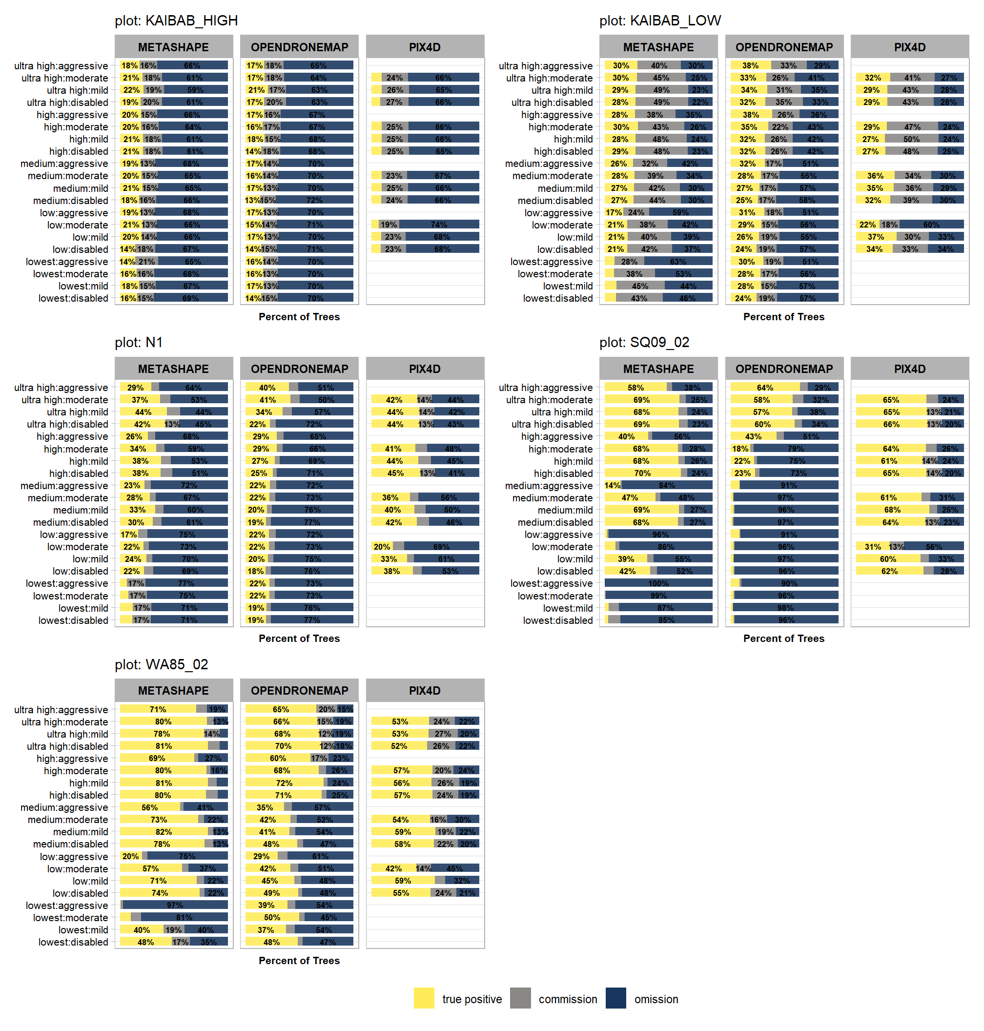

5.6.2 F-score

plt_fn_temp = function(site = study_site_list[1]){
ptcld_validation_data %>%
  dplyr::filter(study_site == site) %>% 
  dplyr::mutate(
    plot_lab = forcats::fct_cross(depth_maps_generation_quality,depth_maps_generation_filtering_mode)
  ) %>% 
  dplyr::mutate(plot_lab = forcats::fct_reorder(
      plot_lab
      , .x = depth_maps_generation_quality
      , .fun = max
    ) %>% forcats::fct_rev()
  ) %>% 
  dplyr::distinct(software,plot_lab,f_score) %>%
ggplot(
  mapping = aes(x = f_score, y = plot_lab, fill=f_score, label = scales::comma(f_score, accuracy = 0.01))
) +
  geom_col(
    width = 0.7
  ) +
  geom_text(
    color = "black", size = 2.3
    , hjust = -0.1
  ) +
  facet_grid(cols = vars(software)) +
  scale_fill_viridis_c(option = "mako", direction = -1, begin = 0.1, limits = c(0,max(ptcld_validation_data$f_score)*1.14)) +
  scale_x_continuous(limits = c(0,max(ptcld_validation_data$f_score)*1.14), breaks = NULL) +
  labs(
    fill = ""
    , y = ""
    , x = "F-Score"
    # , title = "UAS and Stem-Mapped Tree F-Score Summary"
    , subtitle = paste0("plot: ", site)
  ) +
  theme_light() +
  theme(
    legend.position = "none"
    , axis.title.x = element_text(size=8, face = "bold")
    , axis.title.y = element_blank()
    , axis.text.x = element_blank()
    , axis.text.y = element_text(color = "black",size=8)
    , axis.ticks.x = element_blank()
    , panel.grid.major.x = element_blank()
    , panel.grid.minor.x = element_blank()
    , strip.text = element_text(color = "black", face = "bold")
  ) +
  guides(
    fill = guide_legend(reverse = T, override.aes = list(alpha = 0.9))
  )
}
# plt_fn_temp()
# map over sites
plt_list_temp = study_site_list %>% 
  purrr::map(plt_fn_temp)
# combine
patchwork::wrap_plots(plt_list_temp, ncol = 2)

5.7 Example Validation Process

Let’s go through one example for KAIBAB_LOW

5.7.1 Data Load

Data load using functions defined above for KAIBAB_LOW

# validation plot boundary
plot_bound_temp = validation_plots %>% 
  dplyr::filter(study_site==study_site_list[2])
# read field data
field_data_temp = read_field_data(my_study_site = study_site_list[2])
# read_uas_data
uas_data_temp = read_uas_data(
  my_processing_id = ptcld_processing_data %>% 
    dplyr::filter(study_site==study_site_list[2]) %>% 
    dplyr::pull(processing_id) %>% 
    .[1]
  , my_crs = sf::st_crs(field_data_temp)
)
# true positive
true_positive_trees_temp = true_positive_trees_fn(uas_data = uas_data_temp, field_data = field_data_temp)
# field_uas_comparison_fn
field_uas_comparison_temp = field_uas_comparison_fn(
  uas_data = uas_data_temp
  , field_data = field_data_temp
  , true_positive_trees = true_positive_trees_temp 
  , plot_data = plot_bound_temp
)

get the orthomosaic (here using from ODM ultra-lowest) from the directory titled field_validation/orthomosaic with the name of the site as the file name (e.g.; “kaibab_high.tif”)

# let's load the orthomosaic for this site too
# put the orthomosaic images (here using from ODM ultra-lowest) in a folder 
# ...titled "field_validation/orthomosaic" with the name of the site as the file ("kaibab_high.tif")
ortho_list = list.files(
  "../data/field_validation/orthomosaic/"
  , pattern = ".*\\.(tif|tiff)$"
  , full.names = T
)
# load raster
ortho_rast = ortho_list %>% 
  purrr::pluck(
    ortho_list %>% 
      toupper() %>% 
      stringr::str_which(pattern = study_site_list[2]) %>% 
      .[1]
  ) %>% 
  terra::rast()
# aggregate to lower resolution if needed
if(terra::res(ortho_rast)[1]<0.5){
  ortho_rast = terra::aggregate(
    ortho_rast
    , fact = round(0.5/terra::res(ortho_rast)[1])
    , fun = "median"
    , cores = round(parallel::detectCores()/2)
  )
}
# ortho_rast
# terra::res(ortho_rast)
# ortho_rast %>%
#   terra::aggregate(2) %>%
#   terra::plotRGB(r = 1, g = 2, b = 3, stretch = "lin", colNA = "transparent")

# convert to stars
ortho_st = ortho_rast %>%  
  terra::subset(subset = c(1,2,3)) %>%
  terra::crop(
    # stand %>% 
    plot_bound_temp %>%
      sf::st_buffer(2) %>% 
      sf::st_bbox() %>% 
      sf::st_as_sfc() %>% 
      terra::vect() %>% 
      terra::project(terra::crs(ortho_rast))
  ) %>% 
  stars::st_as_stars()

# convert to rgb
ortho_rgb = stars::st_rgb(
  ortho_st[,,,1:3]
  , dimension = 3
  , use_alpha = FALSE
  # , stretch = "histogram"
  , probs = c(0.005, 0.995)
  , stretch = "percent"
)

what is all this data?

5.7.2 Orthomosaic Data

ortho_rast

ortho_rast

## class       : SpatRaster 
## dimensions  : 573, 556, 4  (nrow, ncol, nlyr)
## resolution  : 0.5, 0.4999662  (x, y)
## extent      : 380355.9, 380633.9, 4044343, 4044630  (xmin, xmax, ymin, ymax)
## coord. ref. : WGS 84 / UTM zone 12N (EPSG:32612) 
## source(s)   : memory
## names       : red, green, blue, kaibab_low_4 
## min values  :   0,     0,    0,            0 
## max values  : 226,   229,  232,          255

plot it

# ggplot rgb
  plt_rgb = ggplot() +
    stars::geom_stars(data = ortho_rgb[]) +
    scale_fill_identity(na.value = "transparent") + # !!! don't take this out or RGB plot will kill your computer
    # add plot boundary
    geom_sf(
      data =  plot_bound_temp %>%
        terra::vect() %>% 
        terra::project(terra::crs(ortho_rast)) %>% 
        sf::st_as_sf()
      , alpha = 0
      , lwd = 1.2
      , color = "blue"
    ) +
    scale_x_continuous(expand = c(0, 0)) +
    scale_y_continuous(expand = c(0, 0)) +
    labs(
      x = ""
      , y = ""
    ) +
    theme_void()
# plot + boundary
plt_rgb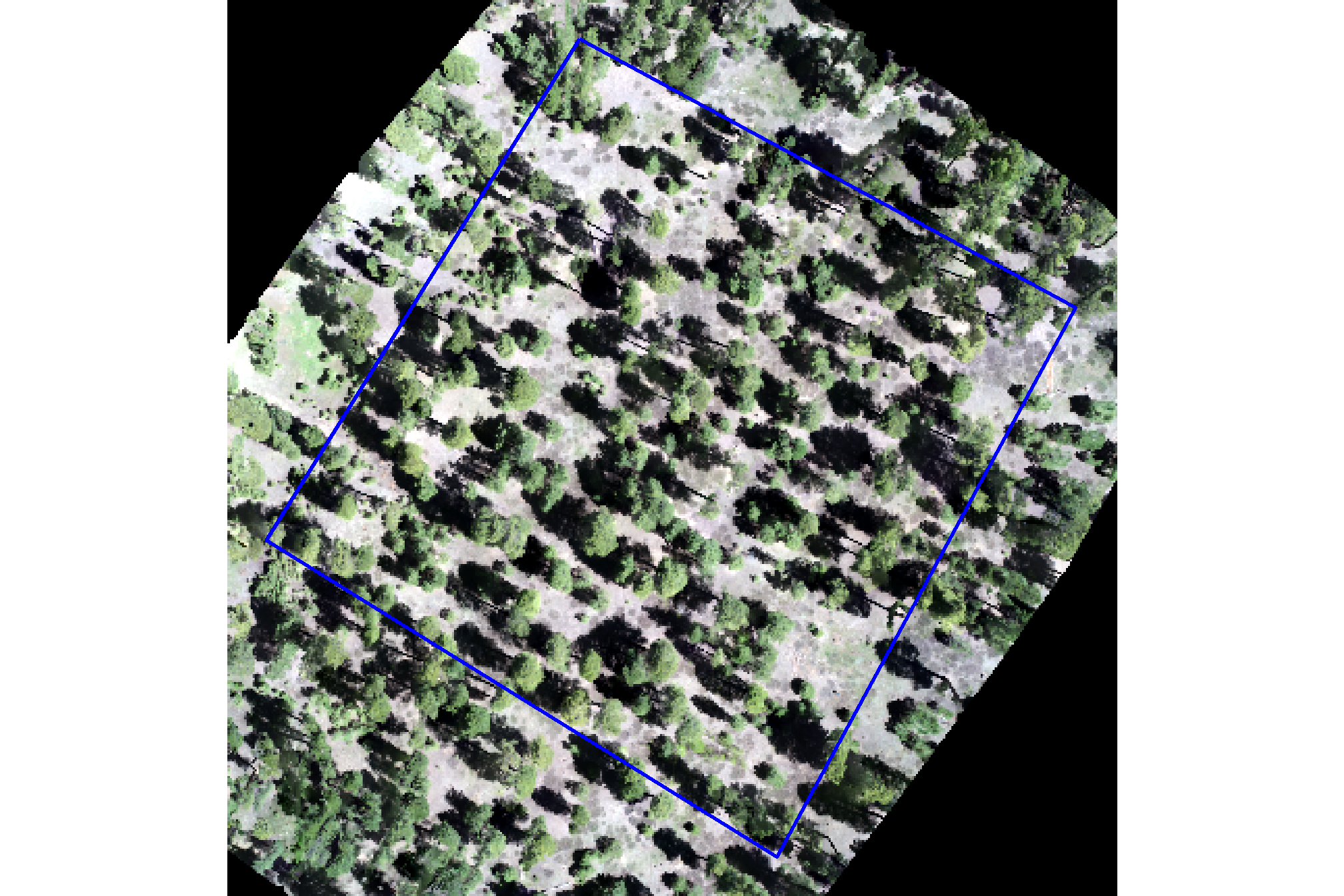

5.7.3 Field Data

field_data

# field_data
field_data_temp %>% dplyr::glimpse()

## Rows: 510
## Columns: 16
## $ field_tree_id              <int> 1, 2, 3, 4, 5, 6, 7, 8, 9, 10, 11, 12, 13, …
## $ site                       <chr> "Kaibab - Low", "Kaibab - Low", "Kaibab - L…
## $ northing                   <dbl> 4044408, 4044405, 4044436, 4044436, 4044443…
## $ easting                    <dbl> 380523.9, 380536.4, 380528.6, 380528.3, 380…
## $ spp                        <chr> "PIPO", "PIPO", "PIPO", "PIPO", "PIPO", "PI…
## $ a.d                        <lgl> NA, NA, NA, NA, NA, NA, NA, NA, NA, NA, NA,…
## $ field_dbh_cm               <dbl> 56.642, 60.960, 13.970, 56.896, 34.544, 45.…
## $ cbh_m                      <dbl> 14.268293, 15.914634, 2.439024, 10.762195, …
## $ field_tree_height_m        <dbl> 26.646341, 24.756098, 6.676829, 23.201220, …
## $ notes                      <chr> NA, NA, NA, NA, NA, NA, NA, NA, NA, NA, NA,…
## $ study_site                 <chr> "KAIBAB_LOW", "KAIBAB_LOW", "KAIBAB_LOW", "…
## $ intersected_with_plot_geom <lgl> TRUE, TRUE, TRUE, TRUE, TRUE, TRUE, TRUE, T…
## $ geometry                   <POINT [m]> POINT (380523.9 4044408), POINT (3805…
## $ tree_utm_x                 <dbl> 380523.9, 380536.4, 380528.6, 380528.3, 380…
## $ tree_utm_y                 <dbl> 4044408, 4044405, 4044436, 4044436, 4044443…
## $ basal_area_m2              <dbl> 0.25198056, 0.29186351, 0.01532790, 0.25424…

plot it

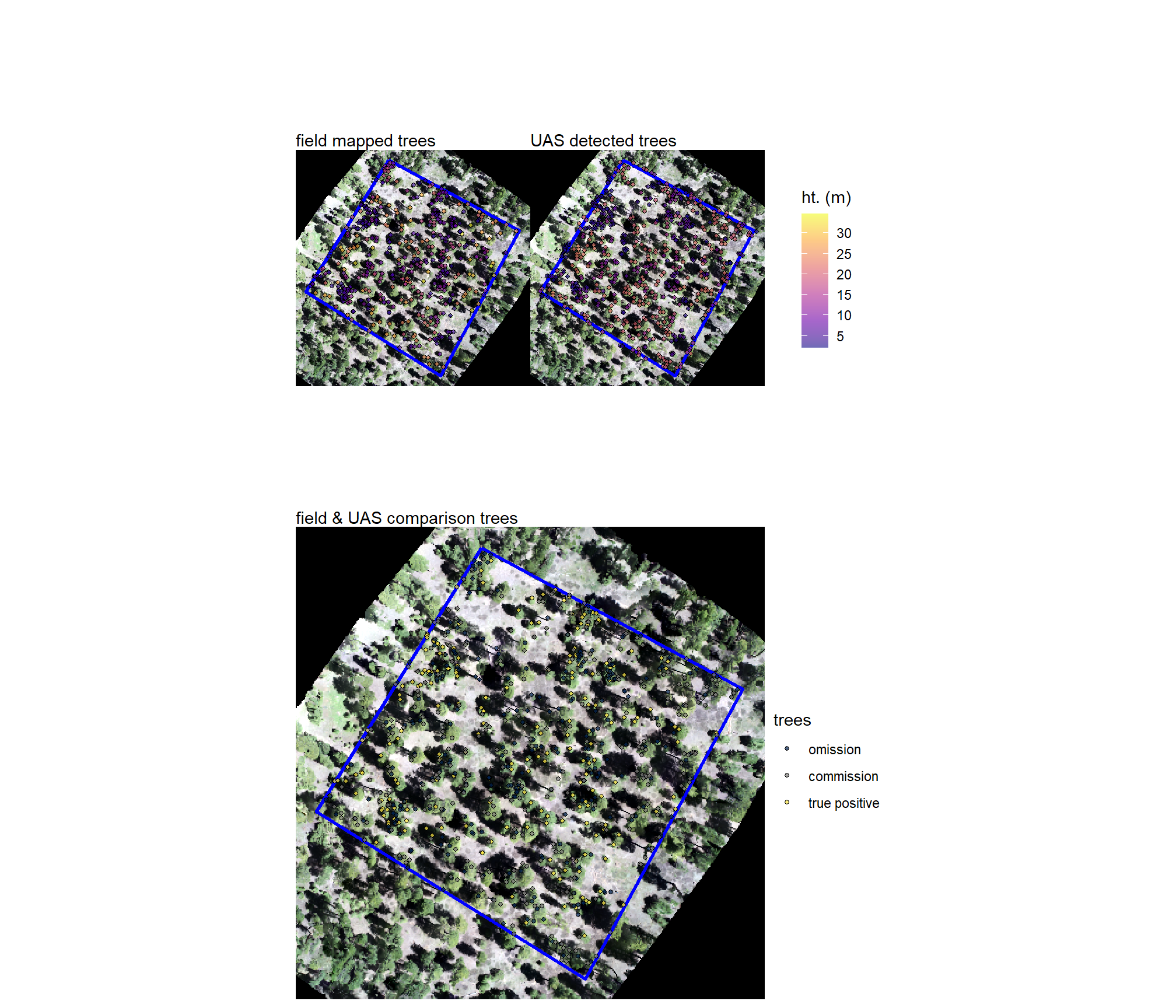
plt_field_data_temp = plt_rgb + 
  ggnewscale::new_scale_fill() +
  geom_sf(
    data = field_data_temp %>% 
      terra::vect() %>% 
      terra::project(terra::crs(ortho_rast)) %>% 
      sf::st_as_sf()
    , mapping = aes(fill = field_tree_height_m)
    , shape = 21
    , size = 1.1
  ) +
  scale_fill_viridis_c(
    option="plasma", alpha = 0.6, name = "ht. (m)"
    , limits = c(
      min(field_data_temp$field_tree_height_m, na.rm = T)
      , max(field_data_temp$field_tree_height_m, na.rm = T)
    )
    , breaks = scales::breaks_extended(6)
  ) + 
  labs(subtitle = "field mapped trees")
# plot
plt_field_data_temp

5.7.4 UAS Data

uas_data

# uas_data
uas_data_temp %>% dplyr::glimpse()

## Rows: 1,592
## Columns: 23
## $ treeid                    <chr> "1_-157075.4_4068915.6", "2_-157089.4_406891…
## $ tree_height_m             <dbl> 5.357, 21.154, 12.778, 21.002, 20.948, 3.579…
## $ crown_area_m2             <dbl> 1.3125, 16.4375, 10.0000, 16.2500, 14.8125, …
## $ comp_trees_per_ha         <dbl> 254.7643, 127.3822, 254.7643, 254.7643, 382.…
## $ comp_relative_tree_height <dbl> 41.92362, 100.00000, 100.00000, 100.00000, 9…
## $ comp_dist_to_nearest_m    <dbl> 4.2500000, 8.4001488, 4.2500000, 2.6575365, …
## $ mean_crown_ht_m           <dbl> 4.122833, 17.681132, 9.023225, 18.342263, 16…
## $ median_crown_ht_m         <dbl> 4.445000, 18.034000, 9.382500, 19.767000, 17…
## $ min_crown_ht_m            <dbl> 2.264000, 12.726000, 3.607500, 8.022000, 3.7…
## $ reg_est_dbh_cm            <dbl> 8.343743, 44.429833, 22.647150, 43.713975, 4…
## $ reg_est_dbh_cm_lower      <dbl> 4.410595, 23.389277, 11.940055, 23.033076, 2…
## $ reg_est_dbh_cm_upper      <dbl> 13.253220, 70.603026, 36.013406, 69.666868, …
## $ is_training_data          <lgl> FALSE, FALSE, FALSE, FALSE, TRUE, FALSE, FAL…
## $ dbh_cm                    <dbl> 8.343743, 44.429833, 22.647150, 43.713975, 4…
## $ dbh_m                     <dbl> 0.4186878, 0.4677839, 0.4125874, 0.4526102, …
## $ radius_m                  <dbl> 0.2093439, 0.2338919, 0.2062937, 0.2263051, …
## $ basal_area_m2             <dbl> 0.005467789, 0.155038385, 0.040282553, 0.150…
## $ basal_area_ft2            <dbl> 0.05885528, 1.66883318, 0.43360140, 1.615489…
## $ processing_id             <int> 21, 21, 21, 21, 21, 21, 21, 21, 21, 21, 21, …
## $ rf_dbh_cm                 <dbl> 41.86878, 46.77839, 41.25874, 45.26102, 43.3…
## $ lin_dbh_cm                <dbl> 20.70054, 47.09968, 30.08387, 46.50466, 43.3…
## $ lin_noint_dbh_cm          <dbl> 2.691027, 51.089210, 10.710425, 49.802237, 4…
## $ geometry                  <POINT [m]> POINT (380503.8 4044624), POINT (38049…

plot it

plt_uas_data_temp = plt_rgb + 
  ggnewscale::new_scale_fill() +
  geom_sf(
    data = uas_data_temp %>% 
      sf::st_transform(sf::st_crs(plot_bound_temp)) %>% 
      sf::st_intersection(plot_bound_temp %>% sf::st_buffer(3)) %>% 
      terra::vect() %>% 
      terra::project(terra::crs(ortho_rast)) %>% 
      sf::st_as_sf()
    , mapping = aes(fill = tree_height_m)
    , shape = 21
    , size = 1.1
  ) +
  scale_fill_viridis_c(
    option="plasma", alpha = 0.6, name = "ht. (m)"
    , limits = c(
      min(field_data_temp$field_tree_height_m, na.rm = T)
      , max(field_data_temp$field_tree_height_m, na.rm = T)
    )
    , breaks = scales::breaks_extended(6)
  ) + 
  labs(subtitle = "UAS detected trees")
# plot
plt_uas_data_temp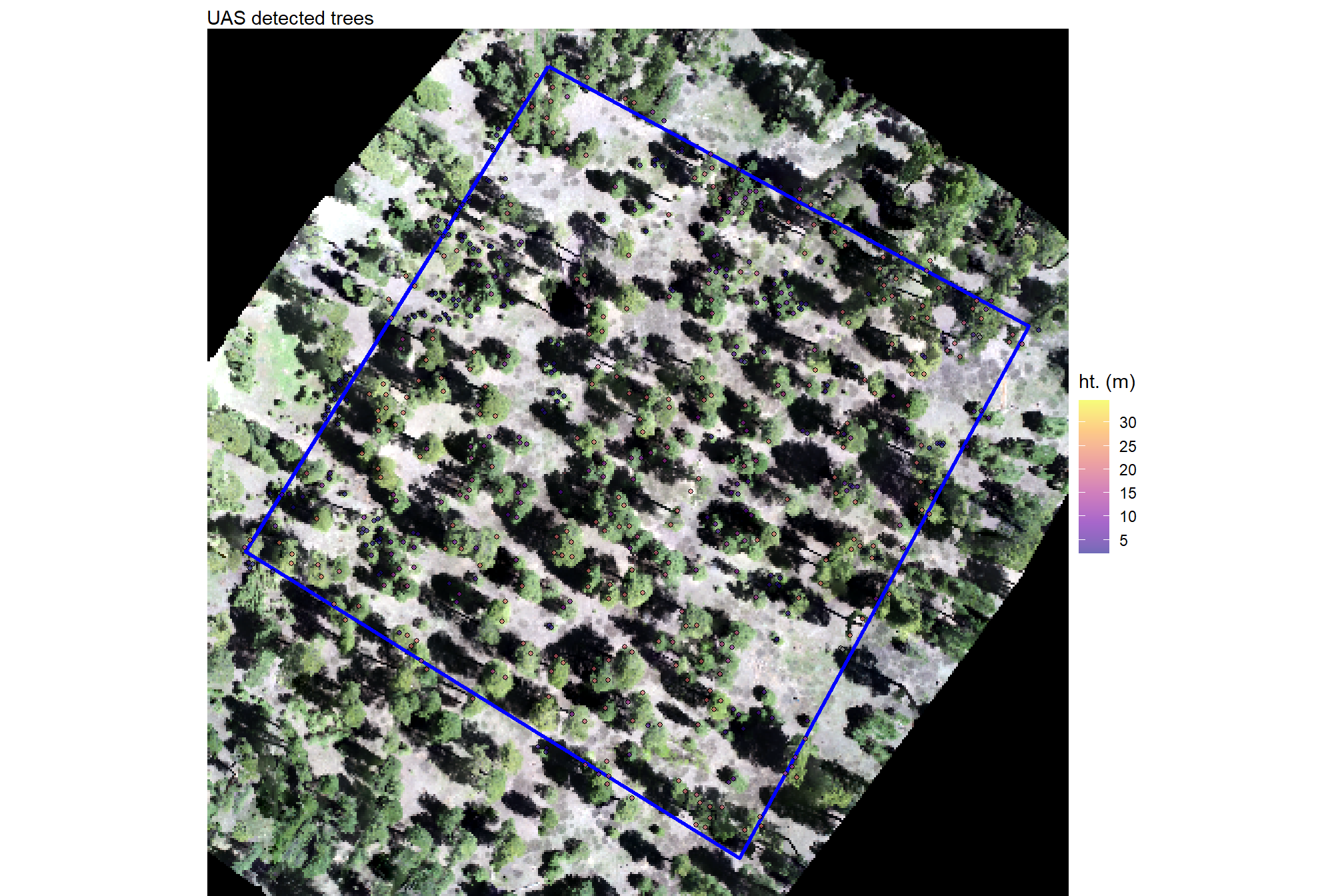

5.7.5 True Positives

true_positive_trees

# true_positive_trees
true_positive_trees_temp %>% dplyr::glimpse()

## Rows: 227
## Columns: 7
## $ uas_tree_id          <chr> "1009_-157051.4_4068750.6", "1014_-157040.9_40687…
## $ field_tree_id        <int> 119, 285, 295, 330, 120, 123, 329, 121, 124, 127,…
## $ uas_tree_height_m    <dbl> 14.261, 21.799, 2.967, 3.563, 18.281, 18.785, 3.2…
## $ field_tree_height_m  <dbl> 14.054878, 22.896341, 2.591463, 3.628049, 17.0731…
## $ height_diff_pct      <dbl> 0.014665487, 0.047926507, 0.144912944, 0.01792942…
## $ field_uas_distance_m <dbl> 1.11155605, 1.11336058, 0.04502782, 0.86474303, 0…
## $ field_uas_group      <chr> "true positive", "true positive", "true positive"…

5.7.6 Field & UAS Comparison

field_uas_comparison

# field_uas_comparison
field_uas_comparison_temp %>% dplyr::glimpse()

## Rows: 818
## Columns: 22
## $ field_uas_group          <ord> true positive, true positive, true positive, …
## $ uas_tree_id              <chr> "1009_-157051.4_4068750.6", "1014_-157040.9_4…
## $ field_tree_id            <dbl> 119, 285, 295, 330, 120, 123, 329, 121, 124, …
## $ height_diff_pct          <dbl> 0.014665487, -0.047926507, 0.144912944, -0.01…
## $ field_uas_distance_m     <dbl> 1.11155605, 1.11336058, 0.04502782, 0.8647430…
## $ uas_dbh_cm               <dbl> 26.245856, 45.977434, 4.981910, 5.755637, 36.…
## $ uas_basal_area_m2        <dbl> 0.054101758, 0.166027239, 0.001949313, 0.0026…
## $ uas_tree_utm_x           <dbl> 380537.9, 380548.3, 380487.0, 380545.8, 38053…
## $ uas_tree_utm_y           <dbl> 4044462, 4044462, 4044454, 4044458, 4044453, …
## $ field_dbh_cm             <dbl> 32.512, 49.276, 4.572, 10.160, 43.434, 30.734…
## $ field_basal_area_m2      <dbl> 0.083018953, 0.190704427, 0.001641732, 0.0081…
## $ field_tree_utm_x         <dbl> 380538.9, 380549.1, 380487.0, 380546.7, 38053…
## $ field_tree_utm_y         <dbl> 4044462, 4044462, 4044454, 4044458, 4044454, …
## $ uas_tree_height_m        <dbl> 14.261, 21.799, 2.967, 3.563, 18.281, 18.785,…
## $ field_tree_height_m      <dbl> 14.054878, 22.896341, 2.591463, 3.628049, 17.…
## $ dbh_diff_cm              <dbl> -6.2661437, -3.2985657, 0.4099102, -4.4043635…
## $ tree_height_diff_m       <dbl> 0.20612163, -1.09734168, 0.37553659, -0.06504…
## $ dbh_diff_pct             <dbl> -0.19273326, -0.06694061, 0.08965665, -0.4335…
## $ abs_dbh_diff_pct         <dbl> 0.19273326, 0.06694061, 0.08965665, 0.4335003…
## $ abs_height_diff_pct      <dbl> 0.014665487, 0.047926507, 0.144912944, 0.0179…
## $ overstory_understory_grp <fct> overstory, overstory, understory, understory,…
## $ overstory_ht_m           <dbl> 7, 7, 7, 7, 7, 7, 7, 7, 7, 7, 7, 7, 7, 7, 7, …

no geometry, let’s attach it

field_uas_comparison_temp = field_uas_comparison_temp %>% 
  dplyr::mutate(
    x = ifelse(!is.na(field_tree_utm_x), field_tree_utm_x, uas_tree_utm_x)
    , y = ifelse(!is.na(field_tree_utm_x), field_tree_utm_y, uas_tree_utm_y)
  ) %>% 
  sf::st_as_sf(
    coords = c("x", "y")
    , crs = sf::st_crs(field_data_temp)
    , remove=T
  )

plot it

plt_comparison_temp = plt_rgb + 
  ggnewscale::new_scale_fill() +
  geom_sf(
    data = field_uas_comparison_temp %>% 
      terra::vect() %>% 
      terra::project(terra::crs(ortho_rast)) %>% 
      sf::st_as_sf()
    , mapping = aes(fill = field_uas_group)
    , color = "black"
    , shape = 21
    , size = 1.1
  ) +
  scale_fill_viridis_d(option = "cividis", name = "trees", drop = F, alpha = 0.7) +
  labs(subtitle = "field & UAS comparison trees")
# plot
plt_comparison_temp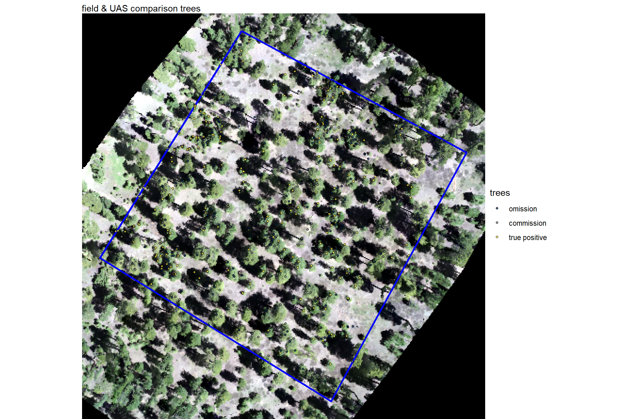

5.7.7 Combine Plots

combine these

(plt_field_data_temp + theme(legend.position = "none") + plt_uas_data_temp) / plt_comparison_temp

ggplot2::ggsave("../data/field_uas_comparison.jpg", width = 8, height = 9)

we can also view these with satellite imagery which is not what the UAS-derived tree detections are from but can be a good viewing tool

# load chm
chm_temp = ptcld_processing_data %>% 
  dplyr::filter(study_site==study_site_list[2]) %>% 
  dplyr::filter(dplyr::row_number()==1) %>% 
  dplyr::mutate(
    f = paste0(
      processed_data_dir
      , "/"
      , file_name
      , "_chm_0.25m.tif"
    )
  ) %>% 
  dplyr::pull(f) %>% 
  terra::rast() %>% 
  terra::aggregate(2) %>% 
  stars::st_as_stars()

# map it
mapview::mapviewOptions(basemaps = c("Esri.WorldImagery", "OpenStreetMap"))
mapview::mapview(
  plot_bound_temp
  , color = "blue"
  , lwd = 2
  , alpha.regions = 0
  , layer.name = "boundary"
  , label = FALSE
  , legend = FALSE
  , popup = FALSE
) +
# aggregate raster and map
  mapview::mapview(
    chm_temp 
    , layer.name = "canopy ht. (m)"
    , col.regions = viridis::plasma(n=50)
    , alpha.regions = 0.7
    , na.color = "transparent"
  ) +
# validation
  mapview::mapview(
    field_uas_comparison_temp
    , zcol = "field_uas_group"
    , col.regions = viridis::cividis(n=3)
    , cex = 2
    , alpha.regions = 0.8
    , layer.name = "validation"
    , popup = leafpop::popupTable(
      field_uas_comparison_temp
      , zcol = c(
        "field_uas_group"
        , "uas_tree_height_m"
        , "field_tree_height_m"
        , "uas_dbh_cm"
        , "field_dbh_cm"
      )
      , row.numbers = FALSE
      , feature.id = FALSE
    )
  ) + 
# fld
  mapview::mapview(
    field_data_temp
    , zcol = "field_tree_height_m"
    , cex = 2
    , alpha.regions = 0.8
    , layer.name = "field"
    , hide = T
  )+ 
# uas
  mapview::mapview(
    uas_data_temp
    , zcol = "tree_height_m"
    , cex = 2
    , alpha.regions = 0.8
    , layer.name = "uas"
    , hide = T
  )

5.7.8 Height vs. DBH of \(Tp\), \(Co\), \(Om\)

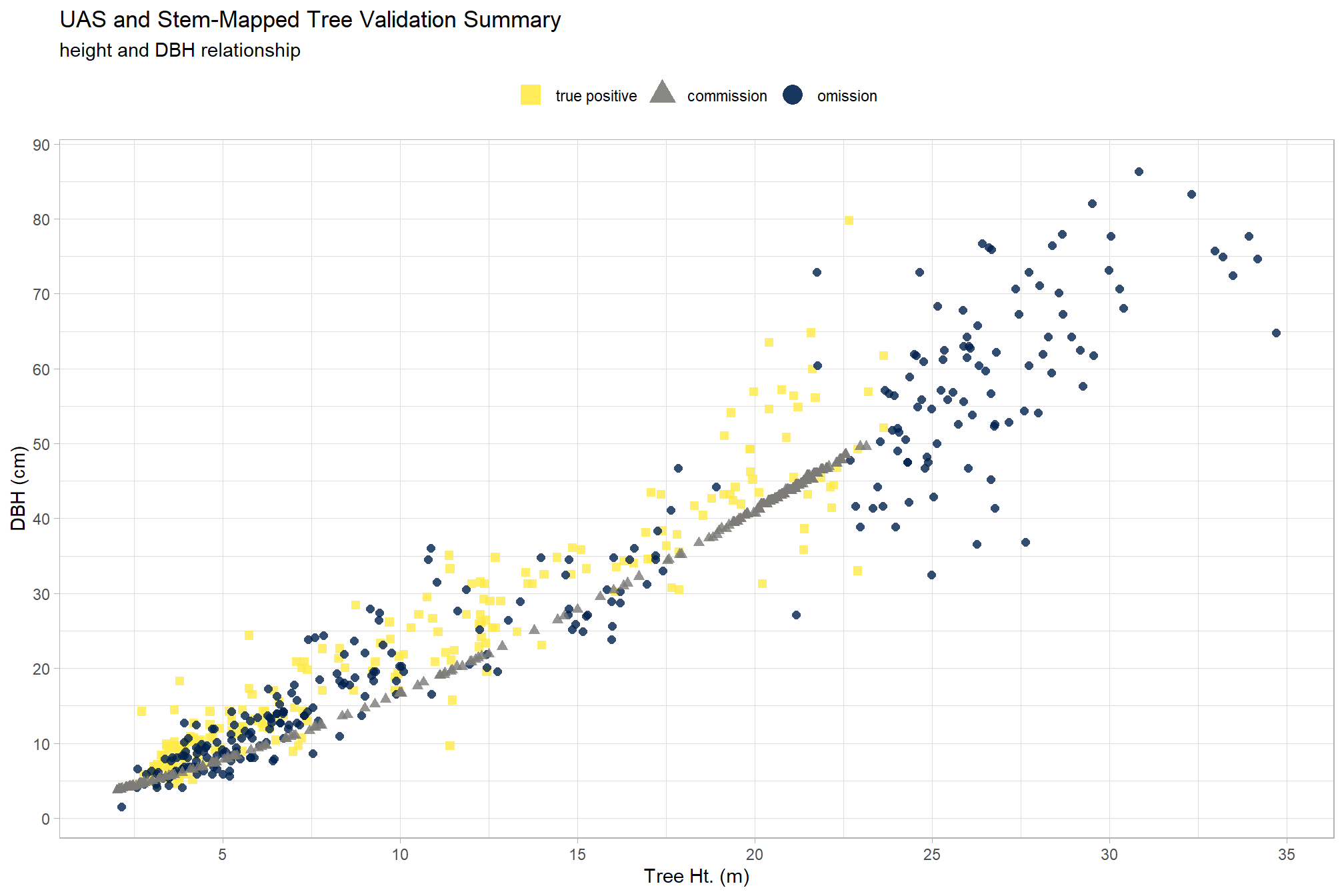
field_uas_comparison_temp %>% 
  sf::st_drop_geometry() %>% 
  dplyr::mutate(
    dbh_temp = dplyr::coalesce(field_dbh_cm, uas_dbh_cm)
    , ht_temp = dplyr::coalesce(field_tree_height_m, uas_tree_height_m)
  ) %>% 
  ggplot(
    mapping = aes(x = ht_temp, y = dbh_temp, color = field_uas_group)
  ) +
    geom_point(
      mapping = aes(shape = field_uas_group)
      , alpha=0.8
      , size=2
    ) +
    scale_color_viridis_d(option = "cividis", drop = F) +
    scale_x_continuous(breaks = scales::extended_breaks(n=8)) +
    scale_y_continuous(breaks = scales::extended_breaks(n=8)) +
    labs(
      color = "detection"
      , shape = "detection"
      , y = "DBH (cm)"
      , x = "Tree Ht. (m)"
      , title = "UAS and Stem-Mapped Tree Validation Summary"
      , subtitle = "height and DBH relationship"
    ) +
    theme_light() +
    theme(
      legend.position = "top"
      , legend.direction  = "horizontal"
      , legend.title = element_blank()
    ) +
    guides(
      color = guide_legend(reverse = T, override.aes = list(alpha = 0.9, size = 5))
      , shape = guide_legend(reverse = T)
    )  

5.7.9 Height and DBH Distribution \(Tp\), \(Co\), \(Om\)

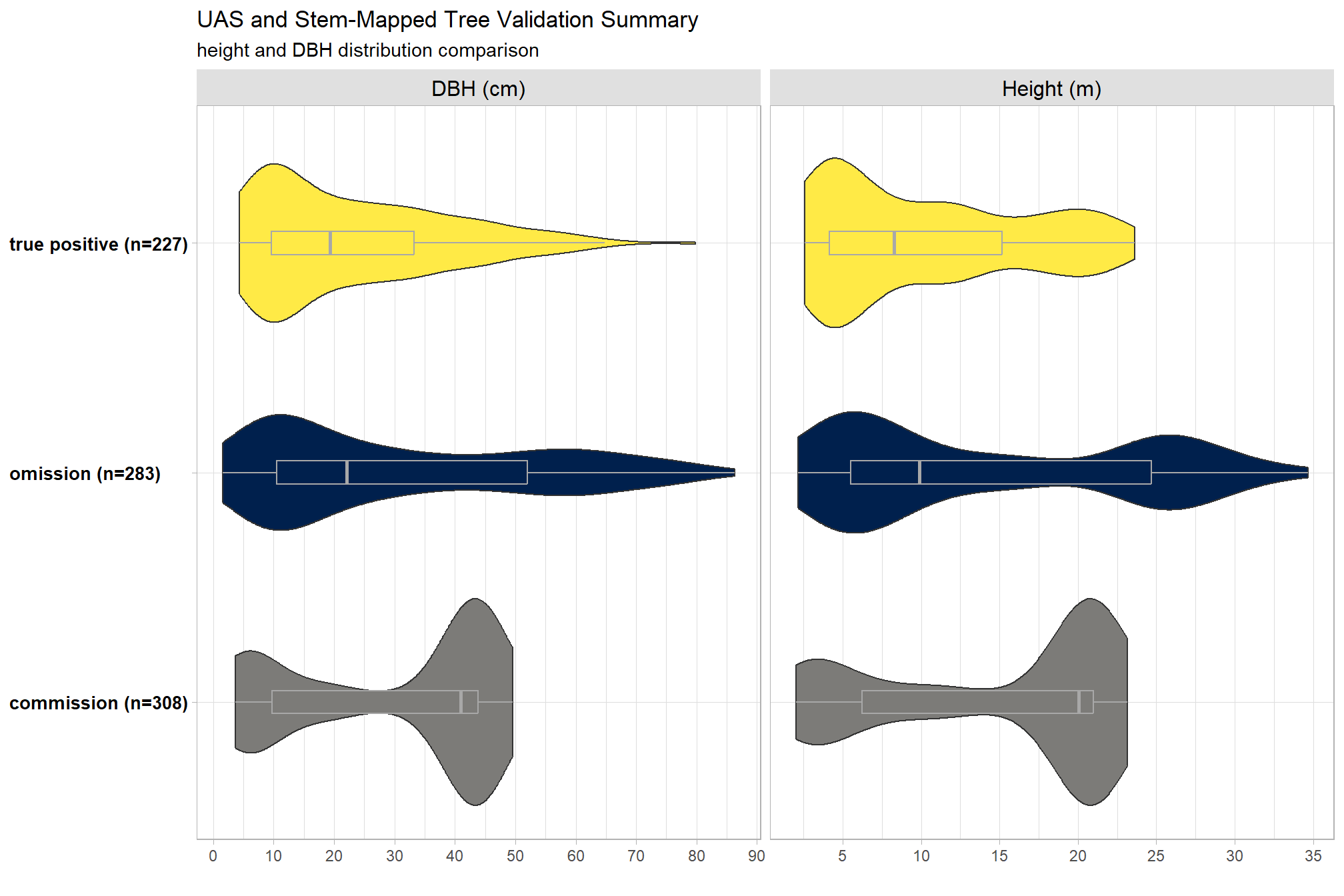
field_uas_comparison_temp %>% 
  sf::st_drop_geometry() %>% 
  dplyr::mutate(
    dbh = dplyr::coalesce(field_dbh_cm, uas_dbh_cm)
    , height = dplyr::coalesce(field_tree_height_m, uas_tree_height_m)
  ) %>% 
  dplyr::select(dbh, height, field_uas_group) %>% 
  tidyr::pivot_longer(cols = -c(field_uas_group), names_to = "metric", values_to = "value") %>% 
  dplyr::group_by(field_uas_group,metric) %>% 
  dplyr::mutate(
    metric = dplyr::case_when(
      metric == "dbh" ~ "DBH (cm)"
      , metric == "height" ~ "Height (m)"
    )
    , n_rows = dplyr::n()
    , plot_lab = paste0(
      field_uas_group
      ," (n=", scales::comma(n_rows,accuracy=1),")"
    )
  ) %>% 
  ggplot(mapping = aes(x = value, y = plot_lab, fill = field_uas_group)) +
    geom_violin() +
    geom_boxplot(width = 0.1, outlier.shape = NA, color = "gray66") +
    facet_grid(cols = vars(metric), scales = "free_x") +
    scale_fill_viridis_d(option = "cividis", drop = F) +
    scale_x_continuous(breaks = scales::extended_breaks(n=8)) +
    labs(
      fill = ""
      , y = ""
      , x = ""
      , title = "UAS and Stem-Mapped Tree Validation Summary"
      , subtitle = "height and DBH distribution comparison"
    ) +
    theme_light() +
    theme(
      legend.position = "none"
      , axis.title.x = element_text(size=10, face = "bold")
      , axis.title.y = element_blank()
      , axis.text.y = element_text(color = "black",size=10, face = "bold", hjust = 0)
      , strip.text = element_text(color = "black", size = 12)
      , strip.background = element_rect(fill = "gray88")
    )

5.7.10 Detected Overstory (\(TP\)) Height Difference

Detected overstory tree (\(TP\)) height reliability.

field_uas_comparison_temp %>%
  sf::st_drop_geometry() %>% 
  dplyr::filter(field_uas_group == "true positive") %>%
  dplyr::group_by(field_uas_group) %>% 
  dplyr::mutate(
    plot_lab = paste0(
      field_uas_group
      ," (n=", scales::comma(dplyr::n(),accuracy=1),")"
    )
    , med = median(height_diff_pct, na.rm=T)
    , color_box = med<0
  ) %>% 
  ggplot(mapping = aes(x = height_diff_pct)) + # height_diff_pct
  # ggplot(mapping = aes(x = height_diff_pct, y = plot_lab )) + # height_diff_pct
    geom_vline(xintercept = 0, color = "gray22", lwd = 1) +
    # geom_boxplot(mapping = aes(fill = color_box), alpha = 0.8, width = 0.7, outlier.shape = NA) +
    geom_density(mapping = aes(fill = color_box), alpha = 0.8) +
    geom_vline(aes(xintercept = med), color = "gray66", linetype = "dashed") + # ymin = -Inf, ymax = Inf
    geom_text(
      aes(x = med, y = 0, label = paste0("median: ",scales::percent(med, accuracy = 0.1)))
      , hjust = -0.1, vjust = 1
    ) +
    scale_fill_manual(values = c("steelblue", "coral")) +
    scale_x_continuous(
      labels = scales::percent_format()
      , breaks = scales::extended_breaks(n=8)
      , limits = c(
        -max(field_uas_comparison_temp$abs_height_diff_pct, na.rm = T)
        , max(field_uas_comparison_temp$abs_height_diff_pct, na.rm = T)
      )
    ) +
    scale_y_continuous(NULL, breaks = NULL) +
    labs(
      fill = ""
      , y = ""
      , x = "Percent Difference in Height"
      , title = "Detected Overstory Height Difference"
      , caption = "-values = UAS<field | +values = UAS>field"
    ) +
    theme_light() +
    theme(
      legend.position = "none"
      , axis.title.x = element_text(size=10, face = "bold")
      , axis.title.y = element_blank()
      , axis.text.y = element_text(color = "black",size=10, face = "bold", hjust = 0)
    )

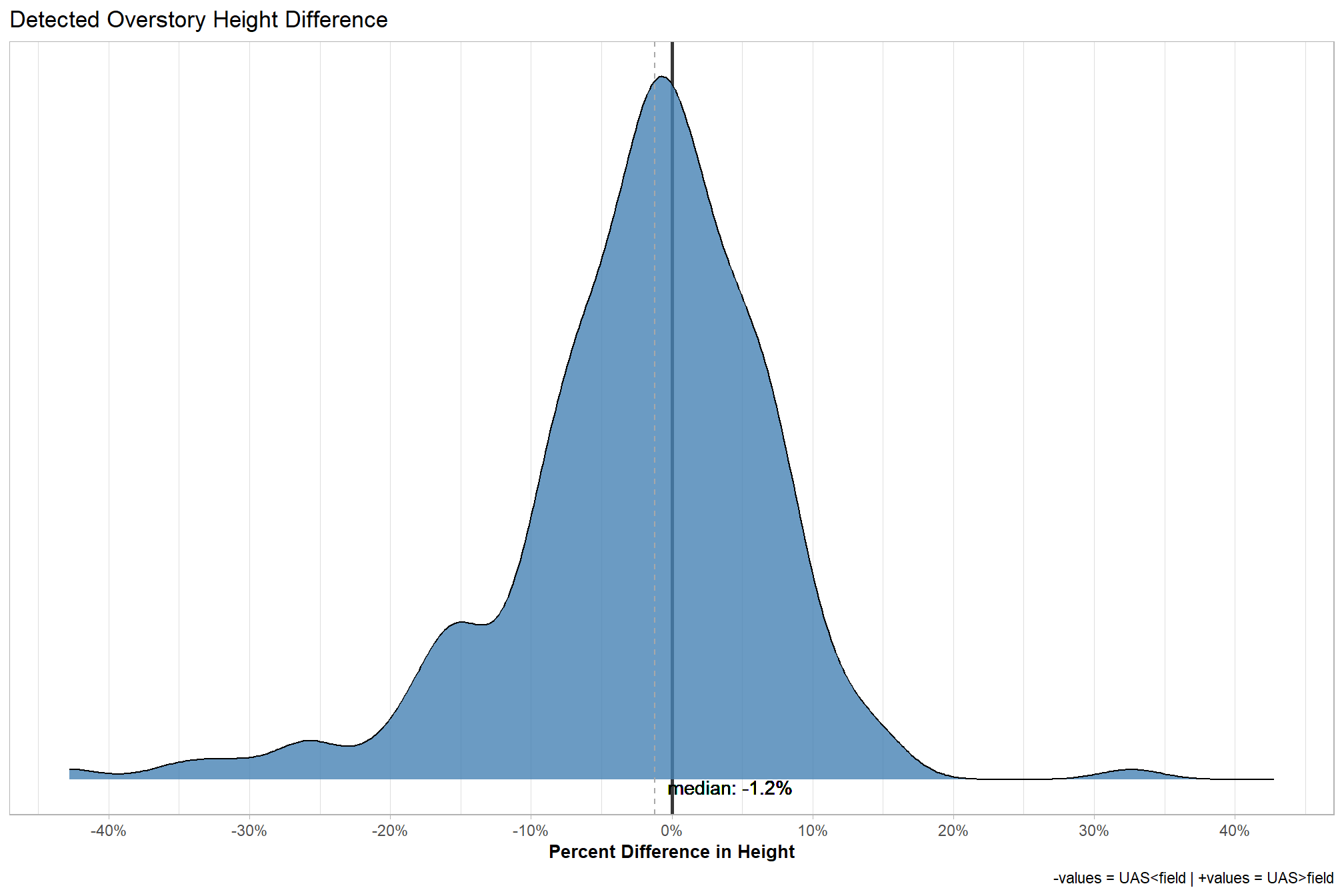
5.7.11 Detected Overstory (\(TP\)) DBH Difference

Detected overstory tree (\(TP\)) DBH reliability.

field_uas_comparison_temp %>%
  sf::st_drop_geometry() %>% 
  dplyr::filter(field_uas_group == "true positive") %>%
  dplyr::group_by(field_uas_group) %>% 
  dplyr::mutate(
    plot_lab = paste0(
      field_uas_group
      ," (n=", scales::comma(dplyr::n(),accuracy=1),")"
    )
    , med = median(dbh_diff_pct, na.rm=T)
    , color_box = med<0
  ) %>% 
  ggplot(mapping = aes(x = dbh_diff_pct)) + # height_diff_pct
    geom_vline(xintercept = 0, color = "gray22", lwd = 1) +
    geom_density(mapping = aes(fill = color_box), alpha = 0.8) +
    geom_vline(aes(xintercept = med), color = "gray66", linetype = "dashed") + # ymin = -Inf, ymax = Inf
    geom_text(
      aes(x = med, y = 0, label = paste0("median: ",scales::percent(med, accuracy = 0.1)))
      , hjust = -0.1, vjust = 1
    ) +
    scale_fill_manual(values = c("steelblue", "coral")) +
    scale_x_continuous(
      labels = scales::percent_format()
      , breaks = scales::extended_breaks(n=8)
      , limits = c(-2,2)
    ) +
    scale_y_continuous(NULL, breaks = NULL) +
    labs(
      fill = ""
      , y = ""
      , x = "Percent Difference in DBH"
      , title = "Detected Overstory DBH Difference"
      , caption = "-values = UAS<field | +values = UAS>field"
    ) +
    theme_light() +
    theme(
      legend.position = "none"
      , axis.title.x = element_text(size=10, face = "bold")
      , axis.title.y = element_blank()
      , axis.text.y = element_text(color = "black",size=10, face = "bold", hjust = 0)
    )

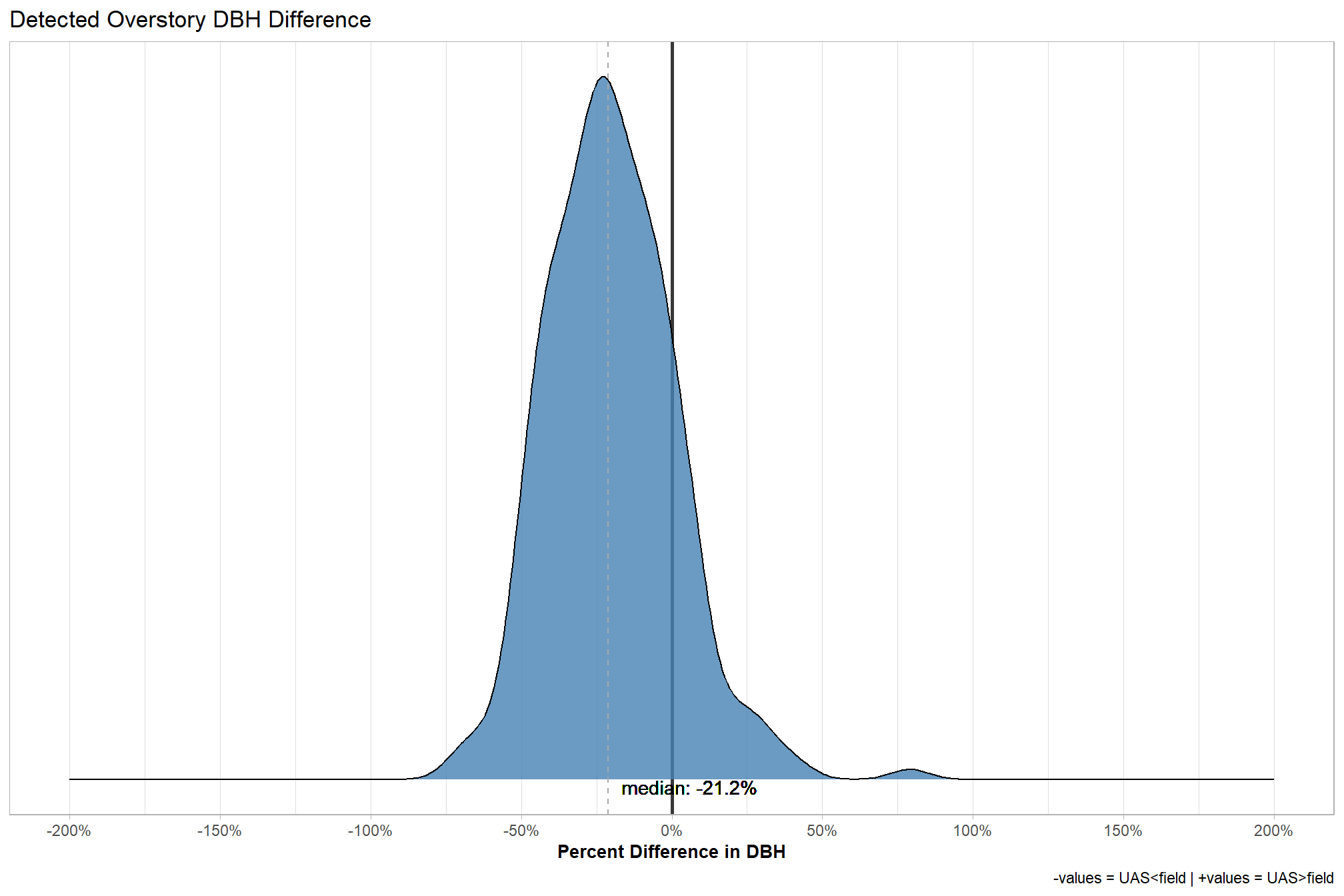
5.7.11.1 Detected Overstory (\(TP\)) Reliability

dbh_f_temp = field_uas_comparison_temp %>% dplyr::filter(field_uas_group=="true positive") %>% dplyr::pull(field_dbh_cm)
dbh_u_temp = field_uas_comparison_temp %>% dplyr::filter(field_uas_group=="true positive") %>% dplyr::pull(uas_dbh_cm)
ht_f_temp = field_uas_comparison_temp %>% dplyr::filter(field_uas_group=="true positive") %>% dplyr::pull(field_tree_height_m)
ht_u_temp = field_uas_comparison_temp %>% dplyr::filter(field_uas_group=="true positive") %>% dplyr::pull(uas_tree_height_m)

data.frame(
  mae_dbh = Metrics::mae(
    dbh_f_temp
    , dbh_u_temp
  )
  , mape_dbh = Metrics::mape(
    dbh_f_temp
    , dbh_u_temp
  )
  , rmse_dbh = Metrics::rmse(
    dbh_f_temp
    , dbh_u_temp
  )
    ## height
  , mae_height = Metrics::mae(
    ht_f_temp
    , ht_u_temp
  )
  , mape_height = Metrics::mape(
    ht_f_temp
    , ht_u_temp
  )
  , rmse_height = Metrics::rmse(
    ht_f_temp
    , ht_u_temp
  )
) %>% 
  tidyr::pivot_longer(dplyr::everything()) %>% 
  tidyr::separate_wider_delim(cols = name, delim = "_", names = c("error", "metric")) %>% 
  tidyr::pivot_wider(names_from = error, values_from = value) %>% 
  dplyr::mutate(
    metric = dplyr::case_when(
      metric == "dbh" ~ "DBH (cm)"
      , metric == "height" ~ "Height (m)"
    )
    , n = field_uas_comparison_temp %>% dplyr::filter(field_uas_group=="true positive") %>% nrow()
  ) %>% 
    kableExtra::kbl(
      caption = "Detected overstory tree height and DBH prediction performance"
      , col.names = c(
        " "
        , "Mean Abs. Error"
        , "Mean Abs. Percent Error"
        , "Root Mean Squared Error"
        , "N"
      )
      , digits = 2
    ) %>% 
    kableExtra::kable_styling()

Table 5.1: Detected overstory tree height and DBH prediction performance

	Mean Abs. Error	Mean Abs. Percent Error	Root Mean Squared Error	N
DBH (cm)	4.90	0.24	6.64	227
Height (m)	0.56	0.07	0.73	227

5.8 Mapped validation for all sites

Above, we reviewed the process for matching field mapped trees to UAS detected trees to determine true positive (TP) detections, commission (Co), and omission (Om) trees.

Here, we visualize the location of the classified trees for each study site.

We’re only going to use point clouds generated via Metashape with the “high” point cloud generation quality setting and the “mild” filtering setting.

5.8.1 Plotting Function

Let’s define a plotting function to map sites over

plt_validation_fn = function(my_site = study_site_list[1]){
  ############################################
  # validation plot boundary
  ############################################
    plot_bound_temp = validation_plots %>% 
      dplyr::filter(study_site==my_site)
  ############################################
  # field data
  ############################################
    field_data_temp = read_field_data(my_study_site = my_site)
  ############################################
  # orthomosaic
  ############################################
    ortho_list = list.files(
      "../data/field_validation/orthomosaic/"
      , pattern = ".*\\.(tif|tiff)$"
      , full.names = T
    )
    # load raster
    ortho_rast = ortho_list %>% 
      purrr::pluck(
        ortho_list %>% 
          toupper() %>% 
          stringr::str_which(pattern = my_site) %>% 
          .[1]
      ) %>% 
      terra::rast()
    # aggregate to lower resolution if needed
    if(terra::res(ortho_rast)[1]<0.5){
      ortho_rast = terra::aggregate(
        ortho_rast
        , fact = round(0.5/terra::res(ortho_rast)[1])
        , fun = "median"
        , cores = round(parallel::detectCores()/2)
      )
    }
    # convert to stars
    ortho_st = ortho_rast %>%  
      terra::subset(subset = c(1,2,3)) %>%
      terra::crop(
        # stand %>% 
        plot_bound_temp %>%
          sf::st_buffer(2) %>% 
          sf::st_bbox() %>% 
          sf::st_as_sfc() %>% 
          terra::vect() %>% 
          terra::project(terra::crs(ortho_rast))
      ) %>% 
      stars::st_as_stars()
    
    # convert to rgb
    ortho_rgb = stars::st_rgb(
      ortho_st[,,,1:3]
      , dimension = 3
      , use_alpha = FALSE
      # , stretch = "histogram"
      , probs = c(0.005, 0.995)
      , stretch = "percent"
    )
  ############################################
  # load validation data ftw
  ############################################
  field_uas_comparison_temp = ptcld_validation_data %>% 
    dplyr::filter(
      study_site == my_site
      & tolower(software) == "metashape"
      & tolower(depth_maps_generation_quality) == "high"
      & tolower(depth_maps_generation_filtering_mode) == "mild"
    ) %>% 
    dplyr::pull(validation_file_full_path) %>% 
    readr::read_csv() %>% 
    dplyr::mutate(
      field_uas_group = factor(
          field_uas_group
          , ordered = T
          , levels = c(
            "true positive"
            , "commission"
            , "omission"
          )
        ) %>% forcats::fct_rev()
      , overstory_understory_grp = overstory_understory_grp %>% factor()
      , x = ifelse(!is.na(field_tree_utm_x), field_tree_utm_x, uas_tree_utm_x)
      , y = ifelse(!is.na(field_tree_utm_x), field_tree_utm_y, uas_tree_utm_y)
    ) %>% 
    sf::st_as_sf(
      coords = c("x", "y")
      , crs = sf::st_crs(field_data_temp)
      , remove=T
    )  
  ############################################
  # plot it all
  ############################################
    # make a label
    hey_lab = ptcld_validation_data %>% 
      dplyr::filter(
        study_site == my_site
        & tolower(software) == "metashape"
        & tolower(depth_maps_generation_quality) == "high"
        & tolower(depth_maps_generation_filtering_mode) == "mild"
      ) %>% 
      dplyr::mutate(
        hey_lab = paste0(
          "true positive: ", scales::comma(true_positive_n_trees, accuracy = 1)
          , "\ncommission: ", scales::comma(commission_n_trees, accuracy = 1)
          , "\nomission: ", scales::comma(omission_n_trees, accuracy = 1)
          , "\n(F-score: ", scales::comma(f_score, accuracy = 0.01), ")"
        )
      ) %>% 
      dplyr::pull(hey_lab)
    # ggplot rgb
      plt_rgb = ggplot() +
        stars::geom_stars(data = ortho_rgb[]) +
        scale_fill_identity(na.value = "transparent") + # !!! don't take this out or RGB plot will kill your computer
        # add plot boundary
        geom_sf(
          data =  plot_bound_temp %>%
            terra::vect() %>% 
            terra::project(terra::crs(ortho_rast)) %>% 
            sf::st_as_sf()
          , alpha = 0
          , lwd = 1.2
          , color = "blue"
        ) +
        scale_x_continuous(expand = c(0, 0)) +
        scale_y_continuous(expand = c(0, 0)) +
        labs(
          x = ""
          , y = ""
        ) +
        theme_void()
    # combine
      plt_comparison_temp = plt_rgb + 
        ggnewscale::new_scale_fill() +
        geom_sf(
          data = field_uas_comparison_temp %>% 
            terra::vect() %>% 
            terra::project(terra::crs(ortho_rast)) %>% 
            sf::st_as_sf()
          , mapping = aes(fill = field_uas_group)
          , color = "black"
          , shape = 21
          , size = 1.4
        ) +
        scale_fill_viridis_d(option = "cividis", name = "trees", drop = F, alpha = 0.8) +
        labs(
          title = paste0("plot: ", my_site)
          , subtitle = hey_lab
        ) +
        theme(legend.position = "bottom", legend.direction = "horizontal")
    # return
    return(plt_comparison_temp)
}
# plt_validation_fn(study_site_list[5])

apply the function

hey_list_temp = study_site_list %>% 
  purrr::map(plt_validation_fn)

5.8.2 Validation Maps

hey_list_temp

## [[1]]

## 
## [[2]]

## 
## [[3]]

## 
## [[4]]

## 
## [[5]]

5.8.3 Validation Maps Combined

# combine
patchwork::wrap_plots(hey_list_temp, ncol = 2, guides = "collect") &
  theme(legend.position="bottom", legend.direction = "horizontal", plot.title = element_text(size = 8), plot.subtitle = element_text(size = 7))

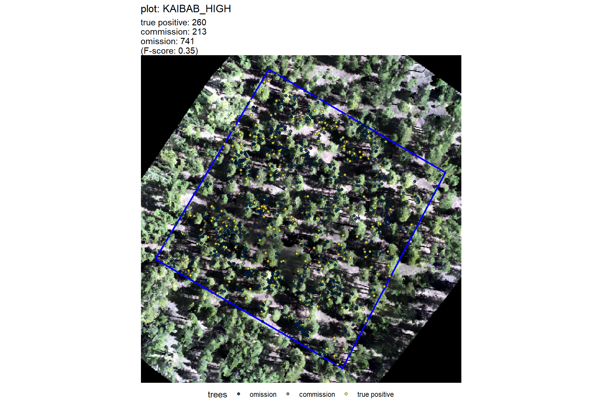
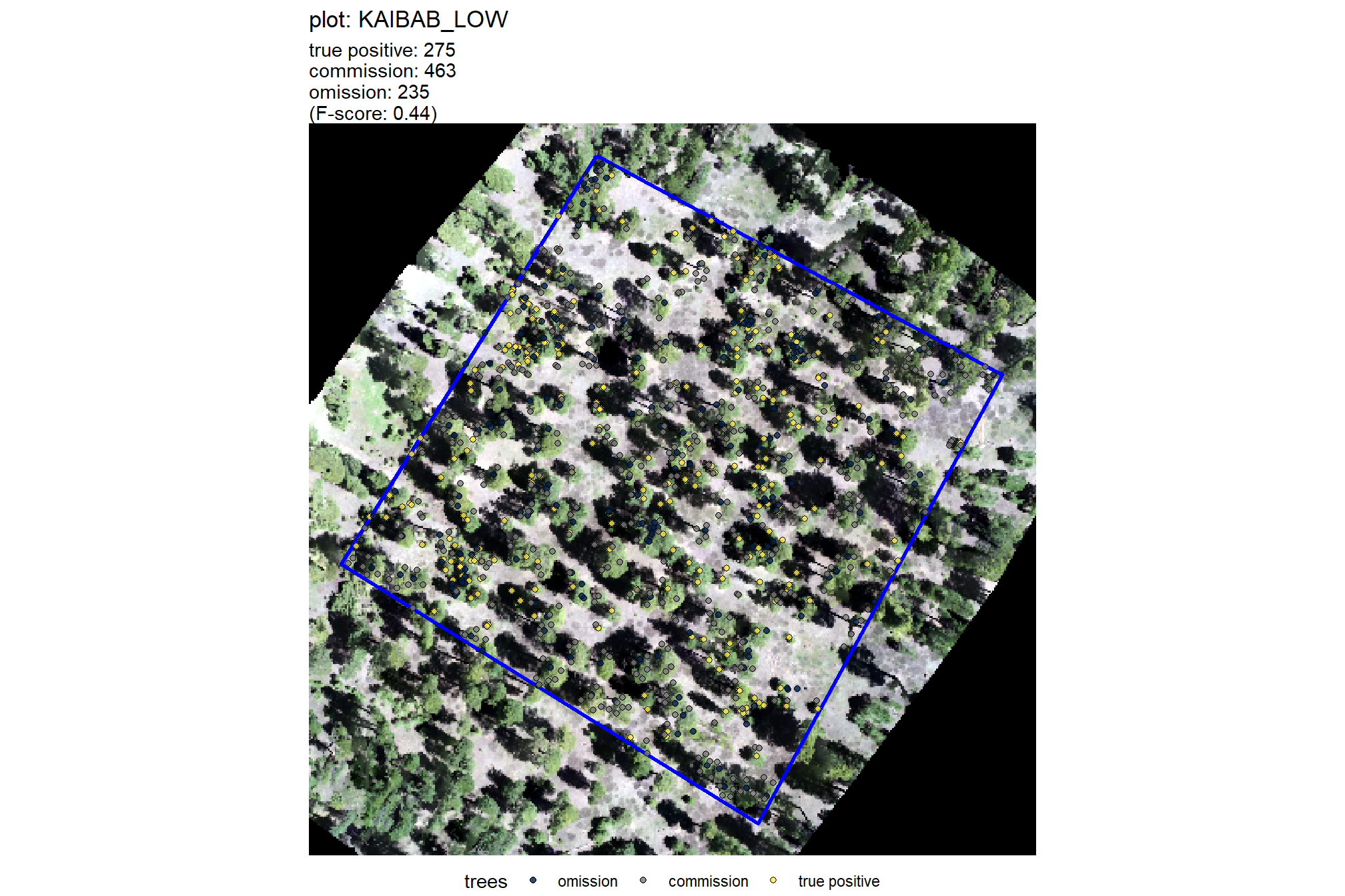
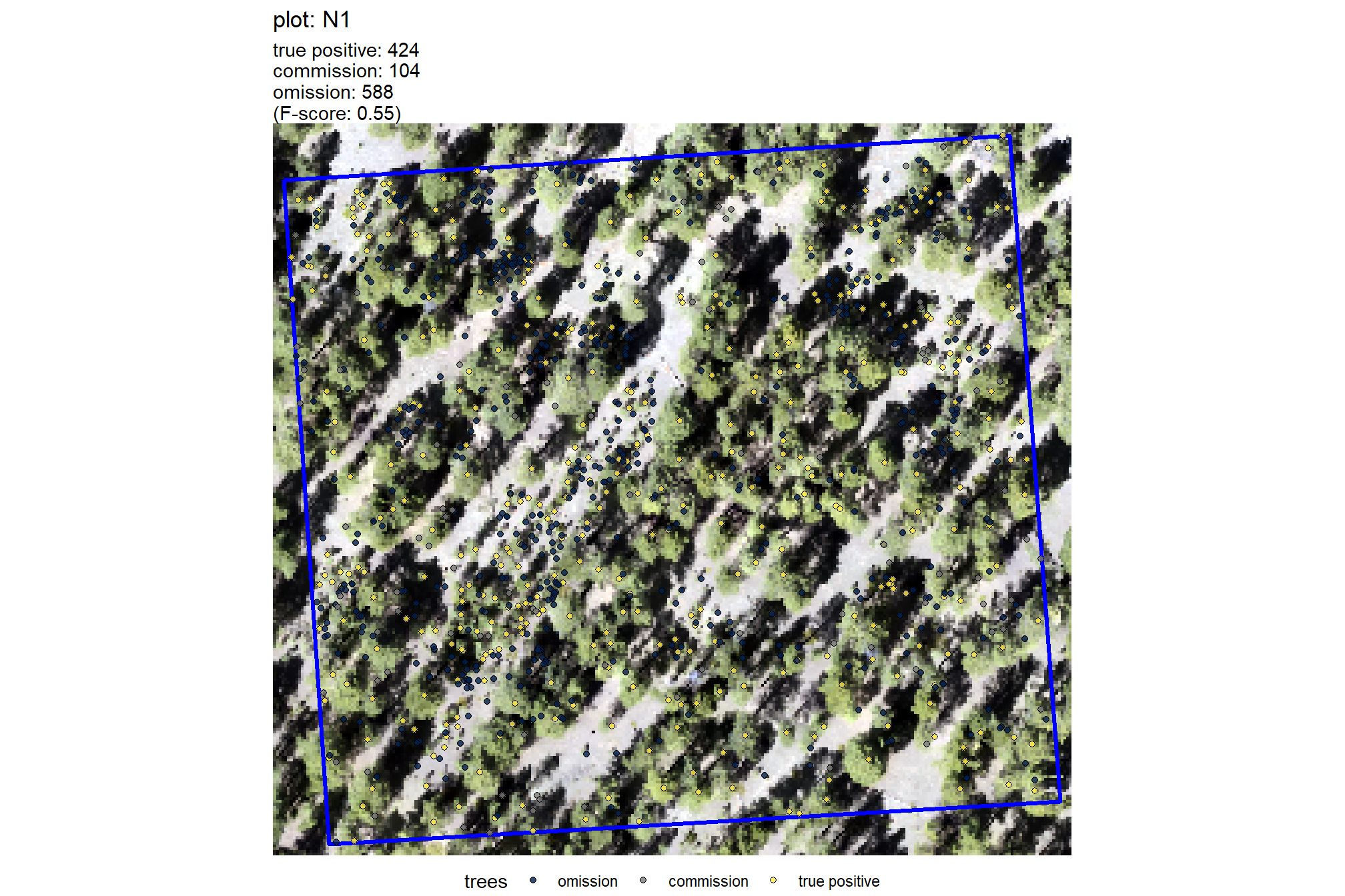
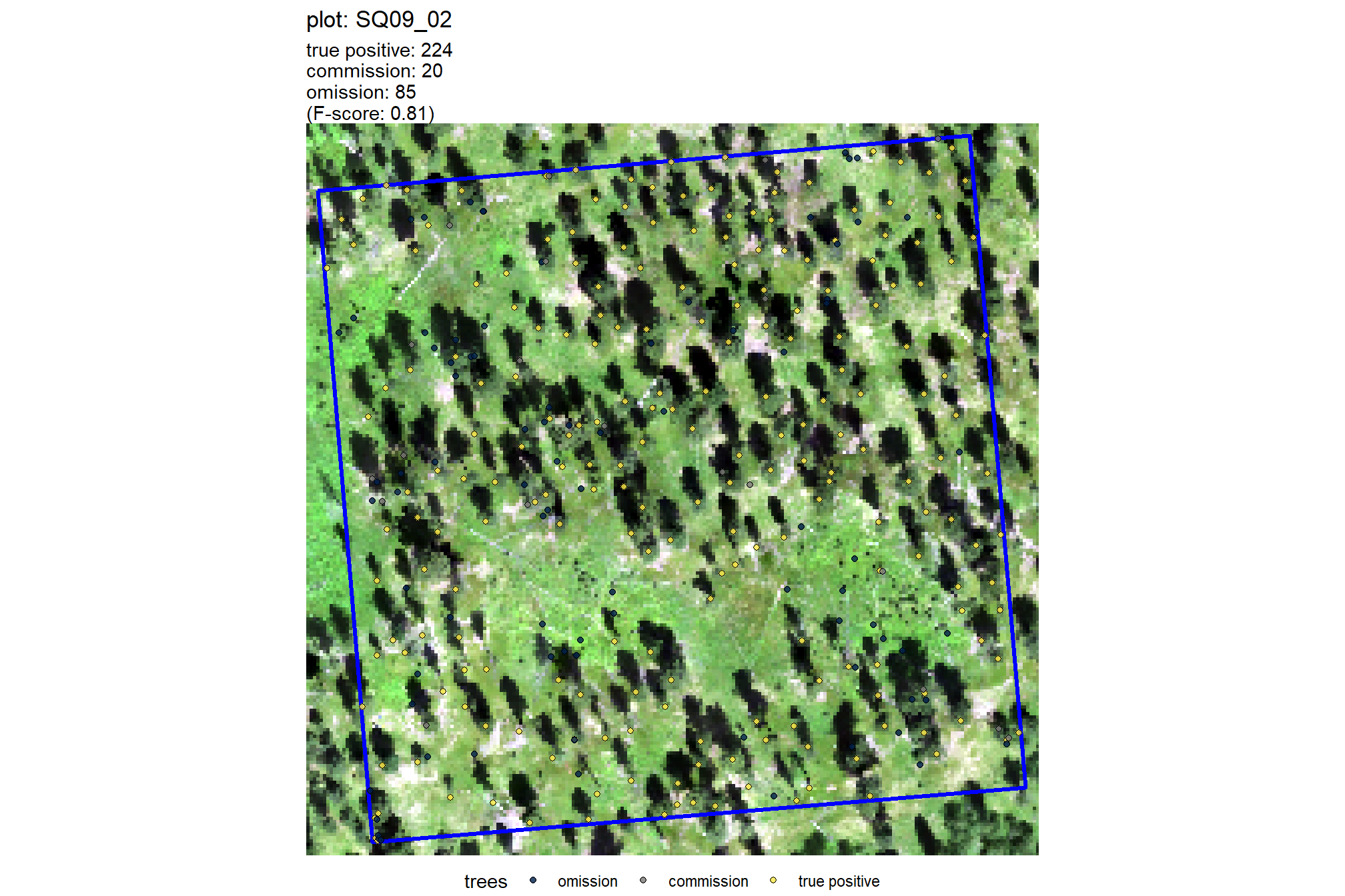
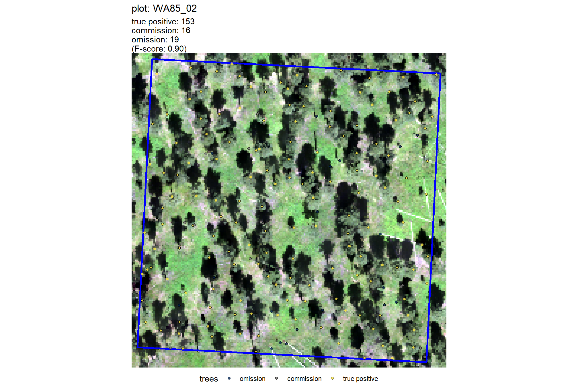
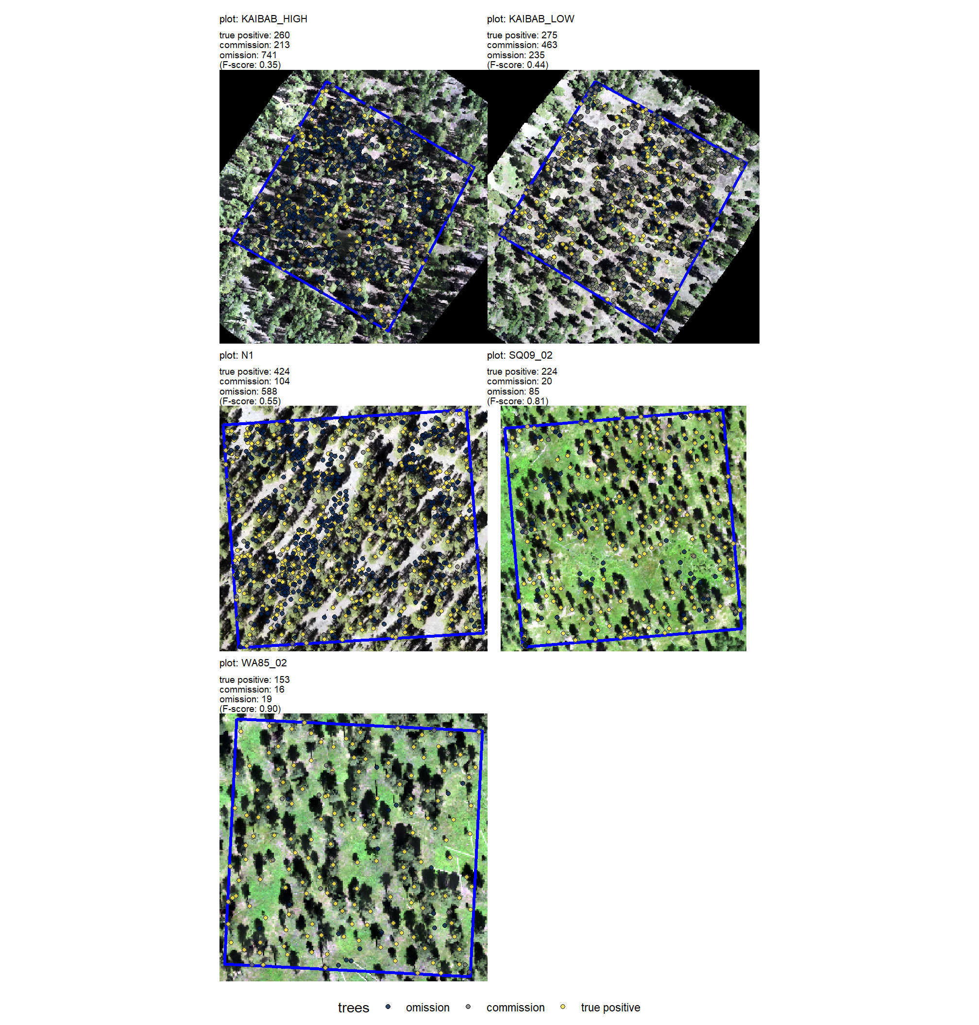
5.9 Field Data Descriptive Statistics

Load and combine all field data sets

field_data = study_site_list %>% 
  purrr::map(function(x){
    read_field_data(x) %>% sf::st_drop_geometry()
  }) %>% 
  dplyr::bind_rows() %>% 
  dplyr::left_join(
    validation_plots %>% 
      dplyr::mutate(ha = sf::st_area(.) %>% as.numeric() %>% `/`(10000)) %>% 
      sf::st_drop_geometry() %>% 
      dplyr::select(study_site, ha)
    , by = dplyr::join_by("study_site")
  )

5.9.1 Table of Height Summary Statistics

field_data %>% 
  dplyr::group_by(study_site,ha) %>% 
  dplyr::summarise(
    n_trees = dplyr::n()
    , min_tree_height_m = min(field_tree_height_m, na.rm = T)
    , max_tree_height_m = max(field_tree_height_m, na.rm = T)
    , median_tree_height_m = median(field_tree_height_m, na.rm = T)
    , tree_height_m_25 = quantile(field_tree_height_m, probs = 0.25)
    , tree_height_m_75 = quantile(field_tree_height_m, probs = 0.75)
  ) %>% 
  dplyr::mutate(
    tph = (n_trees/ha) %>% scales::comma(accuracy = 1)
    ,  n_trees = n_trees %>% scales::comma(accuracy = 1)
  ) %>% 
  dplyr::relocate(tph, .after = n_trees) %>% 
  dplyr::select(-c(ha)) %>% 
  kableExtra::kbl(
    caption = "Field Data: Table of Height Summary Statistics"
    , col.names = c(
      "Site"
      , "# trees"
      , "TPH"
      , "Minimum"
      , "Maximum"
      , "Median"
      , "25th percentile"
      , "75th percentile"
    )
    , digits = 1
  ) %>% 
  kableExtra::add_header_above(
    c(
      " " = 3
      , "Tree Height (meters)"=5
    )
  ) %>%
  kableExtra::kable_styling()

Table 5.2: Field Data: Table of Height Summary Statistics

			Tree Height (meters)
Site	# trees	TPH	Minimum	Maximum	Median	25th percentile	75th percentile
KAIBAB_HIGH	1,001	574	2.1	32.3	11.8	6.8	17.9
KAIBAB_LOW	510	247	2.1	34.7	9.3	4.9	19.9
N1	1,012	639	2.0	26.6	4.9	2.9	14.1
SQ09_02	309	308	2.1	20.7	12.6	7.1	14.7
WA85_02	172	172	2.2	22.9	18.4	10.2	19.9

5.9.2 Table of DBH Summary Statistics

field_data %>% 
  dplyr::group_by(study_site,ha) %>% 
  dplyr::summarise(
    n_trees = dplyr::n()
    , min_dbh_cm = min(field_dbh_cm, na.rm = T)
    , max_dbh_cm = max(field_dbh_cm, na.rm = T)
    , median_dbh_cm = median(field_dbh_cm, na.rm = T)
    , dbh_cm_25 = quantile(field_dbh_cm, probs = 0.25)
    , dbh_cm_75 = quantile(field_dbh_cm, probs = 0.75)
  ) %>% 
  dplyr::mutate(
    tph = (n_trees/ha) %>% scales::comma(accuracy = 1)
    ,  n_trees = n_trees %>% scales::comma(accuracy = 1)
  ) %>% 
  dplyr::relocate(tph, .after = n_trees) %>% 
  dplyr::select(-c(ha)) %>% 
  kableExtra::kbl(
    caption = "Field Data: Table of DBH Summary Statistics"
    , col.names = c(
      "Site"
      , "# trees"
      , "TPH"
      , "Minimum"
      , "Maximum"
      , "Median"
      , "25th percentile"
      , "75th percentile"
    )
    , digits = 1
  ) %>% 
  kableExtra::add_header_above(
    c(
      " " = 3
      , "Tree DBH (cm)"=5
    )
  ) %>%
  kableExtra::kable_styling()

Table 5.3: Field Data: Table of DBH Summary Statistics

			Tree DBH (cm)
Site	# trees	TPH	Minimum	Maximum	Median	25th percentile	75th percentile
KAIBAB_HIGH	1,001	574	1.8	106.7	18.8	11.2	32.5
KAIBAB_LOW	510	247	1.5	86.4	20.3	10.0	41.7
N1	1,012	639	1.0	63.2	7.1	3.3	25.7
SQ09_02	309	308	1.0	41.4	21.6	15.0	25.4
WA85_02	172	172	2.3	53.1	36.1	24.8	39.6

5.9.3 Height and DBH Distribution

field_data %>% 
  dplyr::select(study_site, field_dbh_cm, field_tree_height_m) %>% #
  tidyr::pivot_longer(
    cols = -c(study_site)
  ) %>% 
  dplyr::mutate(
    name = dplyr::case_when(
      name == "field_dbh_cm" ~ "DBH (cm)"
      , name == "field_tree_height_m" ~ "Height (m)"
      , T ~ "error"
    )
  ) %>% 
  # plot
  ggplot(mapping = aes(x = value, y = study_site)) +
    geom_violin(mapping = aes(fill = name), color = NA) +
    geom_boxplot(width = 0.1, outlier.shape = NA, fill = NA, color = "black") +
    facet_grid(cols = vars(name), scales = "free_x") +
    scale_fill_manual(values = c("skyblue4", "skyblue2")) +
    scale_x_continuous(breaks = scales::breaks_extended(8)) +
    labs(x = "", y = "") +
    theme_light() +
    theme(legend.position = "none", strip.text = element_text(color = "black", face = "bold"))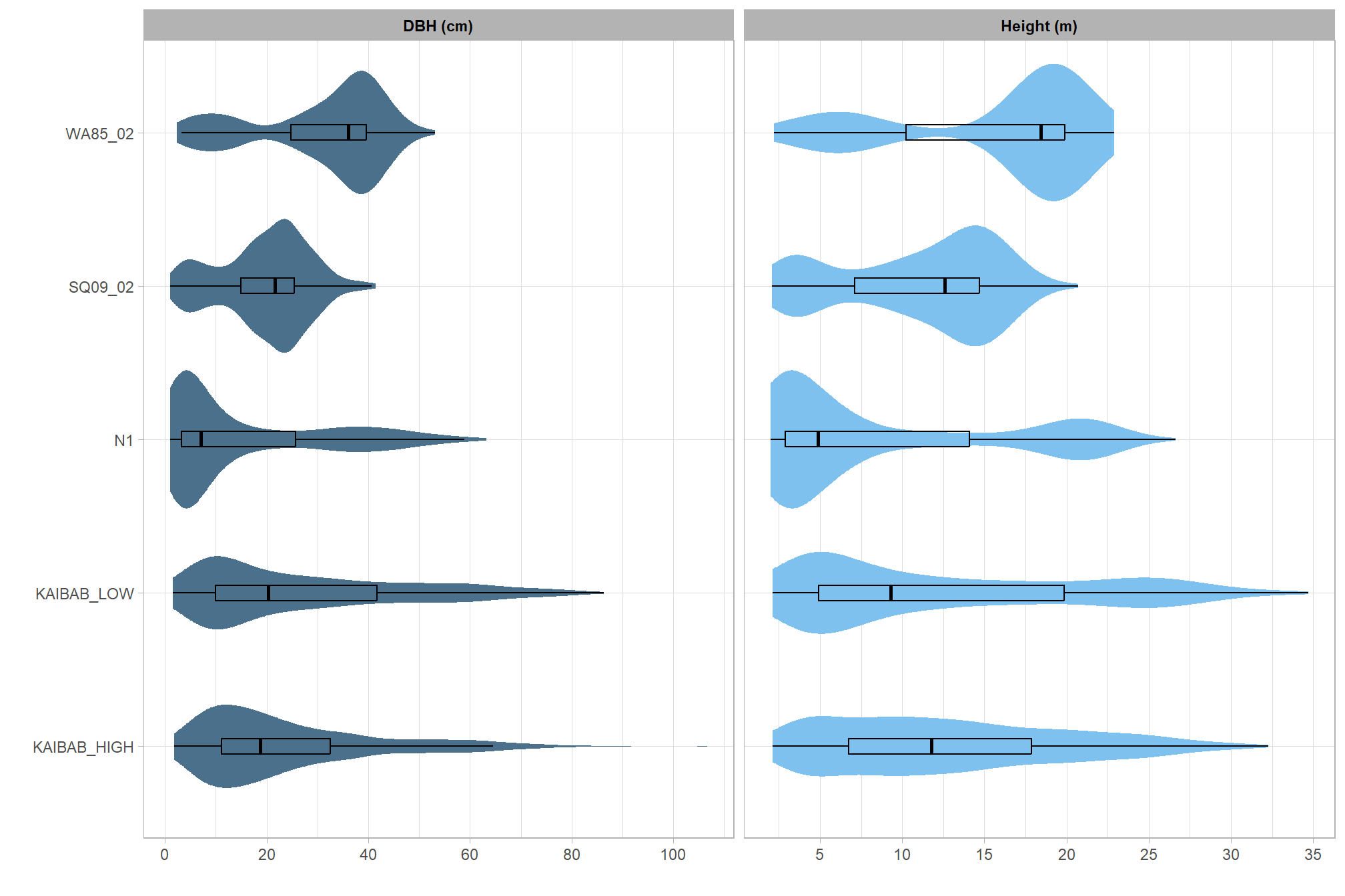

5.10 Summary of Dependent Variables

descriptive statistics of potential dependent variables

ptcld_validation_data %>% 
  dplyr::select(
    f_score, basal_area_pct_error, basal_area_abs_pct_error
    , tree_height_m_me, tree_height_m_rmse, dbh_cm_me, dbh_cm_rmse
  ) %>% 
  dplyr::ungroup() %>% 
  dplyr::summarise(
    dplyr::across(
      .cols = tidyselect::everything()
      , .fns = list(
        mean = ~ mean(.x, na.rm=T)
        , median = ~ median(.x, na.rm=T)
        , sd = ~ sd(.x, na.rm=T)
        , min = ~ min(.x, na.rm=T)
        , max = ~ max(.x, na.rm=T)
      )
      , .names = "{.fn}_xxx_{.col}"
    )
    , n = dplyr::n()
  ) %>% 
  tidyr::pivot_longer(cols = -n) %>% 
  tidyr::separate(col = name, sep = "_xxx_", into = c("stat", "metric")) %>% 
  # format
  dplyr::mutate(
    value = dplyr::case_when(
      stringr::str_detect(metric, "_pct_") ~ scales::percent(value, accuracy = 0.1)
      , metric == "f_score" ~ scales::number(value, accuracy = 0.01)
      , T ~ scales::number(value, accuracy = 0.1)
    )
  ) %>% 
  tidyr::pivot_wider(names_from = stat, values_from = value) %>% 
  dplyr::relocate(c(metric, n)) %>% 
  # dplyr::mutate(
  #   range = paste0(
  #     min, " to ", max
  #   )
  # ) %>% 
  # select(-c(min, max)) 
  kableExtra::kbl(
    digits = 2
    , caption = "SfM data set summary statistics of potential dependent variable metrics"
  ) %>% 
  kableExtra::kable_styling()

Table 5.4: SfM data set summary statistics of potential dependent variable metrics

metric	n	mean	median	sd	min	max
f_score	260	0.46	0.44	0.23	0.00	0.90
basal_area_pct_error	260	-13.1%	-10.4%	33.8%	-100.0%	51.9%
basal_area_abs_pct_error	260	26.3%	19.0%	24.8%	0.3%	100.0%
tree_height_m_me	260	0.1	0.2	0.4	-1.9	0.8
tree_height_m_rmse	260	0.8	0.8	0.2	0.4	1.9
dbh_cm_me	260	0.7	0.1	3.5	-9.7	8.5
dbh_cm_rmse	260	6.3	5.9	2.6	3.3	12.4