Section 7 Statistical Analysis: Detected Tree Reliability
In this section, we’ll evaluate the influence of the processing parameters on UAS-detected tree height and DBH reliability.
The UAS and Field validation data was built and described in this section. For this section we will only look at data from “matched” UAS-field tree pairs (i.e. true positive trees). For successfully matched trees, the UAS tree height and DBH values were compared to field survey tree values to determine the mean error and root mean square error (RMSE). The mean error quantifies the bias of the UAS data while the RMSE quantifies the precision of the UAS data.
We will utilize our “full” model presented in the prior section in which we modeled the F-score which is a measure of how well the UAS detected trees represent the field survey trees.
For a more in-depth review of the traditional treatment of this sort of data structure called multifactor analysis of variance (ANOVA) compared to the Bayesian hierarchical generalization of the traditional ANOVA model used here see this previous section.
7.1 Model Definition
We will used the same model structure for all dependent variables of interest in this section which include:
- Height Mean Error (m)
- Height RMSE (m)
- DBH Mean Error (cm)
- DBH RMSE (cm)
Kruschke (2015) describes the Hierarchical Bayesian approach to describe groups of metric data with multiple nominal predictors when every subject (“study site” in our research) only contributes one observation per cell/condition:
\[\begin{align*} y = & \; \beta_0 \\ & + \overrightarrow \beta_1 \overrightarrow x_1 + \overrightarrow \beta_2 \overrightarrow x_2 + \overrightarrow \beta_{1 \times 2} \overrightarrow x_{1 \times 2} \\ & + \overrightarrow \beta_S \overrightarrow x_S \end{align*}\]
In other words, we assume a main effect of subject, but no interaction of subject with other predictors. In this model, the subject effect (deflection) is constant across treatments, and the treatment effects (deflections) are constant across subjects. Notice that the model makes no requirement that every subject contributes a datum to every condition. Indeed, the model allows zero or multiple data per subject per condition. Bayesian estimation makes no assumptions or requirements that the design is balanced (i.e., has equal numbers of measurement in each cell). (p. 608)
and see section 20 from Kurz’s ebook supplement
The metric predicted variable with three nominal predictor variables and subject-level effects model has the form:
\[\begin{align*} y_{i} \sim & \operatorname{Normal}\bigl(\mu_{i}, \sigma_{y} \bigr) \\ \mu_{i} = & \beta_0 \\ & + \sum_{j=1}^{J=5} \beta_{1[j]} x_{1[j]} + \sum_{k=1}^{K=4} \beta_{2[k]} x_{2[k]} + \sum_{f=1}^{F=3} \beta_{3[f]} x_{3[f]} + \sum_{s=1}^{S=5} \beta_{4[s]} x_{4[s]} \\ & + \sum_{j,k} \beta_{1\times2[j,k]} x_{1\times2[j,k]} + \sum_{j,f} \beta_{1\times3[j,f]} x_{1\times3[j,f]} + \sum_{k,f} \beta_{2\times3[k,f]} x_{2\times3[k,f]} \\ & + \sum_{j,k,f} \beta_{1\times2\times3[j,k,f]} x_{1\times2\times3[j,k,f]} \\ \beta_{0} \sim & \operatorname{Normal}(\bar{y},y_{SD} \times 5) \\ \beta_{1[j]} \sim & \operatorname{Normal}(\bar{y},\sigma_{\beta_{1}}) \\ \beta_{2[k]} \sim & \operatorname{Normal}(\bar{y},\sigma_{\beta_{2}}) \\ \beta_{3[f]} \sim & \operatorname{Normal}(\bar{y},\sigma_{\beta_{3}}) \\ \beta_{4[s]} \sim & \operatorname{Normal}(\bar{y},\sigma_{\beta_{4}}) \\ \beta_{1\times2[j,k]} \sim & \operatorname{Normal}(\bar{y},\sigma_{\beta_{1\times2}}) \\ \beta_{1\times3[j,f]} \sim & \operatorname{Normal}(\bar{y},\sigma_{\beta_{1\times3}}) \\ \beta_{2\times3[k,f]} \sim & \operatorname{Normal}(\bar{y},\sigma_{\beta_{2\times3}}) \\ \sigma_{\beta_{1}} \sim & \operatorname{Gamma}(shape,rate) \\ \sigma_{\beta_{2}} \sim & \operatorname{Gamma}(shape,rate) \\ \sigma_{\beta_{3}} \sim & \operatorname{Gamma}(shape,rate) \\ \sigma_{\beta_{4}} \sim & \operatorname{Gamma}(shape,rate) \\ \sigma_{\beta_{1\times2}} \sim & \operatorname{Gamma}(shape,rate) \\ \sigma_{\beta_{1\times3}} \sim & \operatorname{Gamma}(shape,rate) \\ \sigma_{\beta_{2\times3}} \sim & \operatorname{Gamma}(shape,rate) \\ \sigma_{y} \sim & \operatorname{Cauchy}(0,y_{SD}) \\ \end{align*}\]
, where \(j\) is the depth map generation quality setting corresponding to observation \(i\), \(k\) is the depth map filtering mode setting corresponding to observation \(i\), \(f\) is the processing software corresponding to observation \(i\), and \(s\) is the study site corresponding to observation \(i\)
for this model, we’ll define the priors following Kurz
Kruschke (2015) explains this prior distribution methodology:
we let the data serve as a proxy and we set the prior wide relative to the variance in the data, called
ySD. Analogously, the normal prior for the baselinea0is centered on the data mean and made very wide relative to the variance of the data. The goal is merely to achieve scale invariance, so that whatever is the measurement scale of the data, the prior will be broad and noncommittal on that scale…The prior onaSigmais a gamma distribution that is broad on the scale of the data, and that has a nonzero mode so that its probability density drops to zero asaSigmaapproaches zero. Specifically, the shape and rate parameters of the gamma distribution are set so its mode issd(y)/2and its standard deviation is2*sd(y)(p.560-561)
7.2 Setup
load the data if needed
# load data if needed
if(ls()[ls() %in% "ptcld_validation_data"] %>% length()==0){
 ptcld_validation_data = readr::read_csv("../data/ptcld_full_analysis_data.csv") %>%
   dplyr::mutate(
      depth_maps_generation_quality = factor(
          depth_maps_generation_quality %>%
            tolower() %>%
            stringr::str_replace_all("ultrahigh", "ultra high")
          , ordered = TRUE
          , levels = c(
            "lowest"
            , "low"
            , "medium"
            , "high"
            , "ultra high"
          )
        ) %>% forcats::fct_rev()
      , depth_maps_generation_filtering_mode = factor(
          depth_maps_generation_filtering_mode %>% tolower()
          , ordered = TRUE
          , levels = c(
            "disabled"
            , "mild"
            , "moderate"
            , "aggressive"
          )
        ) %>% forcats::fct_rev()
    )
}
What is this data?
## Rows: 260
## Columns: 114
## $ tracking_file_full_path               <chr> "D:\\SfM_Software_Comparison\\Me…
## $ software                              <chr> "METASHAPE", "METASHAPE", "METAS…
## $ study_site                            <chr> "KAIBAB_HIGH", "KAIBAB_HIGH", "K…
## $ processing_attribute1                 <chr> "HIGH", "HIGH", "HIGH", "HIGH", …
## $ processing_attribute2                 <chr> "AGGRESSIVE", "DISABLED", "MILD"…
## $ processing_attribute3                 <chr> NA, NA, NA, NA, NA, NA, NA, NA, …
## $ file_name                             <chr> "HIGH_AGGRESSIVE", "HIGH_DISABLE…
## $ number_of_points                      <int> 52974294, 72549206, 69858217, 69…
## $ las_area_m2                           <dbl> 86661.27, 87175.42, 86404.78, 86…
## $ timer_tile_time_mins                  <dbl> 0.63600698, 2.49318542, 0.841338…
## $ timer_class_dtm_norm_chm_time_mins    <dbl> 3.6559556, 5.3289152, 5.1638296,…
## $ timer_treels_time_mins                <dbl> 8.9065272, 19.2119663, 12.339179…
## $ timer_itd_time_mins                   <dbl> 0.02202115, 0.02449968, 0.037984…
## $ timer_competition_time_mins           <dbl> 0.10590740, 0.17865245, 0.121248…
## $ timer_estdbh_time_mins                <dbl> 0.02290262, 0.02382533, 0.021991…
## $ timer_silv_time_mins                  <dbl> 0.012565533, 0.015940932, 0.0150…
## $ timer_total_time_mins                 <dbl> 13.361886, 27.276985, 18.540606,…
## $ sttng_input_las_dir                   <chr> "D:/Metashape_Testing_2024", "D:…
## $ sttng_use_parallel_processing         <lgl> FALSE, FALSE, FALSE, FALSE, FALS…
## $ sttng_desired_chm_res                 <dbl> 0.25, 0.25, 0.25, 0.25, 0.25, 0.…
## $ sttng_max_height_threshold_m          <int> 60, 60, 60, 60, 60, 60, 60, 60, …
## $ sttng_minimum_tree_height_m           <int> 2, 2, 2, 2, 2, 2, 2, 2, 2, 2, 2,…
## $ sttng_dbh_max_size_m                  <int> 2, 2, 2, 2, 2, 2, 2, 2, 2, 2, 2,…
## $ sttng_local_dbh_model                 <chr> "rf", "rf", "rf", "rf", "rf", "r…
## $ sttng_user_supplied_epsg              <lgl> NA, NA, NA, NA, NA, NA, NA, NA, …
## $ sttng_accuracy_level                  <int> 2, 2, 2, 2, 2, 2, 2, 2, 2, 2, 2,…
## $ sttng_pts_m2_for_triangulation        <int> 20, 20, 20, 20, 20, 20, 20, 20, …
## $ sttng_normalization_with              <chr> "triangulation", "triangulation"…
## $ sttng_competition_buffer_m            <int> 5, 5, 5, 5, 5, 5, 5, 5, 5, 5, 5,…
## $ depth_maps_generation_quality         <ord> high, high, high, high, low, low…
## $ depth_maps_generation_filtering_mode  <ord> aggressive, disabled, mild, mode…
## $ total_sfm_time_min                    <dbl> 54.800000, 60.316667, 55.933333,…
## $ number_of_points_sfm                  <dbl> 52974294, 72549206, 69858217, 69…
## $ total_sfm_time_norm                   <dbl> 0.1117823680, 0.1237564664, 0.11…
## $ processed_data_dir                    <chr> "D:/SfM_Software_Comparison/Meta…
## $ processing_id                         <int> 1, 2, 3, 4, 5, 6, 7, 8, 9, 10, 1…
## $ true_positive_n_trees                 <dbl> 229, 261, 260, 234, 220, 175, 23…
## $ commission_n_trees                    <dbl> 173, 222, 213, 193, 148, 223, 16…
## $ omission_n_trees                      <dbl> 772, 740, 741, 767, 781, 826, 77…
## $ f_score                               <dbl> 0.3264433, 0.3517520, 0.3527815,…
## $ tree_height_m_me                      <dbl> 0.270336679, 0.283568790, 0.3122…
## $ tree_height_m_mpe                     <dbl> 0.002357383, 0.013286785, 0.0142…
## $ tree_height_m_mae                     <dbl> 0.7873610, 0.6886235, 0.6914983,…
## $ tree_height_m_mape                    <dbl> 0.06624939, 0.06903969, 0.060550…
## $ tree_height_m_smape                   <dbl> 0.06776453, 0.06838733, 0.060410…
## $ tree_height_m_mse                     <dbl> 0.9842433, 0.8507862, 0.8259923,…
## $ tree_height_m_rmse                    <dbl> 0.9920904, 0.9223807, 0.9088412,…
## $ dbh_cm_me                             <dbl> 2.0551269, 1.2718827, 1.7505679,…
## $ dbh_cm_mpe                            <dbl> 0.077076168, 0.056392083, 0.0755…
## $ dbh_cm_mae                            <dbl> 5.091373, 4.375871, 4.674437, 4.…
## $ dbh_cm_mape                           <dbl> 0.2076874, 0.2185989, 0.2110014,…
## $ dbh_cm_smape                          <dbl> 0.1966263, 0.2081000, 0.1986588,…
## $ dbh_cm_mse                            <dbl> 44.38957, 35.29251, 38.33622, 38…
## $ dbh_cm_rmse                           <dbl> 6.662549, 5.940750, 6.191625, 6.…
## $ uas_basal_area_m2                     <dbl> 55.75278, 60.26123, 58.67391, 57…
## $ field_basal_area_m2                   <dbl> 69.04409, 69.04409, 69.04409, 69…
## $ uas_basal_area_m2_per_ha              <dbl> 31.97437, 34.55997, 33.64964, 33…
## $ field_basal_area_m2_per_ha            <dbl> 39.59697, 39.59697, 39.59697, 39…
## $ basal_area_m2_error                   <dbl> -13.291309, -8.782866, -10.37018…
## $ basal_area_m2_per_ha_error            <dbl> -7.622601, -5.036997, -5.947326,…
## $ basal_area_pct_error                  <dbl> -0.19250466, -0.12720663, -0.150…
## $ basal_area_abs_pct_error              <dbl> 0.19250466, 0.12720663, 0.150196…
## $ overstory_commission_n_trees          <dbl> 141, 178, 178, 160, 95, 173, 120…
## $ understory_commission_n_trees         <dbl> 32, 44, 35, 33, 53, 50, 43, 39, …
## $ overstory_omission_n_trees            <dbl> 558, 560, 545, 556, 554, 598, 54…
## $ understory_omission_n_trees           <dbl> 214, 180, 196, 211, 227, 228, 22…
## $ overstory_true_positive_n_trees       <dbl> 185, 183, 198, 187, 189, 145, 19…
## $ understory_true_positive_n_trees      <dbl> 44, 78, 62, 47, 31, 30, 33, 40, …
## $ overstory_f_score                     <dbl> 0.3461179, 0.3315217, 0.3538874,…
## $ understory_f_score                    <dbl> 0.2634731, 0.4105263, 0.3492958,…
## $ overstory_tree_height_m_me            <dbl> 0.41693172, 0.44114110, 0.442167…
## $ understory_tree_height_m_me           <dbl> -0.34602886, -0.08612009, -0.102…
## $ overstory_tree_height_m_mpe           <dbl> 0.020790675, 0.024558478, 0.0241…
## $ understory_tree_height_m_mpe          <dbl> -0.075146232, -0.013158341, -0.0…
## $ overstory_tree_height_m_mae           <dbl> 0.8201433, 0.7820879, 0.7770369,…
## $ understory_tree_height_m_mae          <dbl> 0.6495266, 0.4693415, 0.4183269,…
## $ overstory_tree_height_m_mape          <dbl> 0.04662933, 0.04863237, 0.048708…
## $ understory_tree_height_m_mape         <dbl> 0.14874284, 0.11691842, 0.098369…
## $ overstory_tree_height_m_smape         <dbl> 0.04589942, 0.04776615, 0.047912…
## $ understory_tree_height_m_smape        <dbl> 0.15969736, 0.11676780, 0.100322…
## $ overstory_tree_height_m_mse           <dbl> 1.0623763, 1.0055835, 0.9739823,…
## $ understory_tree_height_m_mse          <dbl> 0.6557300, 0.4876080, 0.3533791,…
## $ overstory_tree_height_m_rmse          <dbl> 1.0307164, 1.0027878, 0.9869054,…
## $ understory_tree_height_m_rmse         <dbl> 0.8097715, 0.6982893, 0.5944570,…
## $ overstory_dbh_cm_me                   <dbl> 2.88225065, 2.37098111, 2.694675…
## $ understory_dbh_cm_me                  <dbl> -1.4225525, -1.3067712, -1.26448…
## $ overstory_dbh_cm_mpe                  <dbl> 0.11199444, 0.09928650, 0.110477…
## $ understory_dbh_cm_mpe                 <dbl> -0.06973931, -0.04424482, -0.035…
## $ overstory_dbh_cm_mae                  <dbl> 5.753010, 5.298094, 5.472454, 5.…
## $ understory_dbh_cm_mae                 <dbl> 2.309487, 2.212192, 2.125931, 2.…
## $ overstory_dbh_cm_mape                 <dbl> 0.1862021, 0.1848729, 0.1898205,…
## $ understory_dbh_cm_mape                <dbl> 0.2980235, 0.2977254, 0.2786439,…
## $ overstory_dbh_cm_smape                <dbl> 0.1686851, 0.1699578, 0.1735200,…
## $ understory_dbh_cm_smape               <dbl> 0.3141064, 0.2975874, 0.2789409,…
## $ overstory_dbh_cm_mse                  <dbl> 52.78250, 46.57941, 47.70797, 46…
## $ understory_dbh_cm_mse                 <dbl> 9.101103, 8.811704, 8.407077, 9.…
## $ overstory_dbh_cm_rmse                 <dbl> 7.265156, 6.824911, 6.907095, 6.…
## $ understory_dbh_cm_rmse                <dbl> 3.016803, 2.968451, 2.899496, 3.…
## $ overstory_uas_basal_area_m2           <dbl> 55.49096, 59.79139, 58.30184, 57…
## $ understory_uas_basal_area_m2          <dbl> 0.2618258, 0.4698415, 0.3720740,…
## $ overstory_field_basal_area_m2         <dbl> 67.50326, 67.50326, 67.50326, 67…
## $ understory_field_basal_area_m2        <dbl> 1.540832, 1.540832, 1.540832, 1.…
## $ overstory_uas_basal_area_m2_per_ha    <dbl> 31.82421, 34.29052, 33.43626, 32…
## $ understory_uas_basal_area_m2_per_ha   <dbl> 0.15015781, 0.26945534, 0.213385…
## $ overstory_field_basal_area_m2_per_ha  <dbl> 38.7133, 38.7133, 38.7133, 38.71…
## $ understory_field_basal_area_m2_per_ha <dbl> 0.883671, 0.883671, 0.883671, 0.…
## $ overstory_basal_area_m2_per_ha_error  <dbl> -6.889088, -4.422782, -5.277041,…
## $ understory_basal_area_m2_per_ha_error <dbl> -0.7335132, -0.6142157, -0.67028…
## $ overstory_basal_area_pct_error        <dbl> -0.17795146, -0.11424450, -0.136…
## $ understory_basal_area_pct_error       <dbl> -0.8300750, -0.6950728, -0.75852…
## $ overstory_basal_area_abs_pct_error    <dbl> 0.17795146, 0.11424450, 0.136310…
## $ understory_basal_area_abs_pct_error   <dbl> 0.8300750, 0.6950728, 0.7585239,…
## $ validation_file_full_path             <chr> "D:/SfM_Software_Comparison/Meta…
## $ overstory_ht_m                        <dbl> 7, 7, 7, 7, 7, 7, 7, 7, 7, 7, 7,…
# a row is unique by...
identical(
nrow(ptcld_validation_data)
, ptcld_validation_data %>%
dplyr::distinct(
study_site, software
, depth_maps_generation_quality
, depth_maps_generation_filtering_mode
, processing_attribute3 # need to align all by software so this will go away or be filled
) %>%
nrow()
)## [1] TRUEload our plotting functions if needed (not showing these functions here but see the prior section for function definitions)
7.3 Tree Height
7.3.1 Summary Statistics
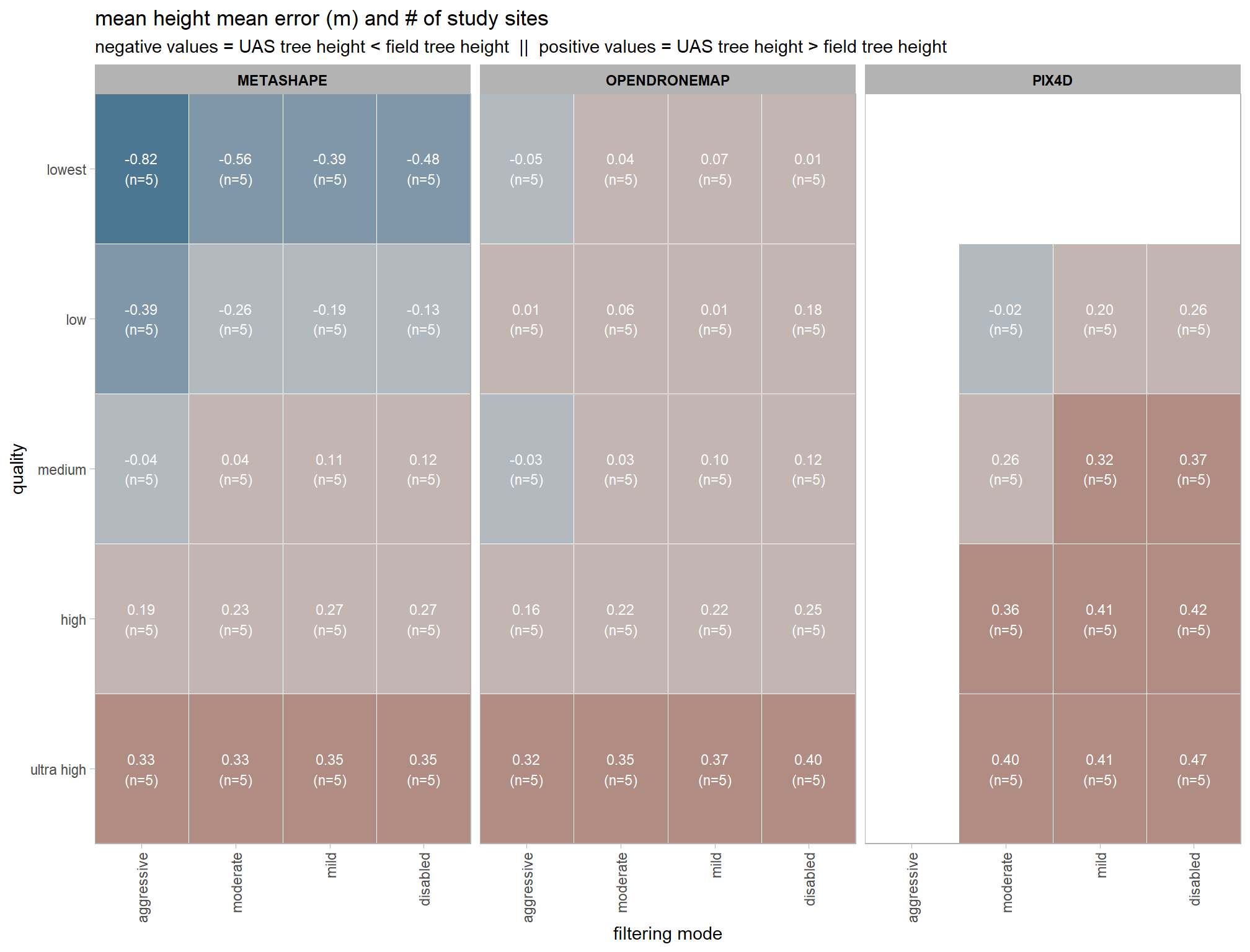
7.3.1.1 Height Mean Error (bias)
  # summarize data
  dta_temp = ptcld_validation_data %>%
    dplyr::group_by(software, depth_maps_generation_quality, depth_maps_generation_filtering_mode) %>%
    # collapse across study site
    dplyr::summarise(
      tree_height_m_me = mean(tree_height_m_me, na.rm = T)
      , n = dplyr::n()
    )
  # set limits for color scale
  lmt_tree_height_m_me = ceiling(10*max(abs(range(dta_temp$tree_height_m_me, na.rm = T))))/10
  # scales::show_col(scales::pal_dichromat("BluetoOrange.10")(10))
  # scales::show_col(scales::pal_div_gradient()(seq(0, 1, length.out = 7)))
  # plot it
  dta_temp %>%
    ggplot(mapping = aes(
      y = depth_maps_generation_quality
      , x = depth_maps_generation_filtering_mode
      , fill = tree_height_m_me
      , label = paste0(scales::comma(tree_height_m_me,accuracy = 0.01), "\n(n=", n,")")
    )) +
    geom_tile(color = "white") +
    geom_text(color = "white", size = 3) +
    facet_grid(cols = vars(software)) +
    scale_x_discrete(expand = c(0, 0)) +
    scale_y_discrete(expand = c(0, 0)) +
    scale_fill_stepsn(
      n.breaks = 7
      , colors = scales::pal_div_gradient()(seq(0, 1, length.out = 7))
      , limits = c(-lmt_tree_height_m_me,lmt_tree_height_m_me)
      , labels = scales::comma_format(accuracy = 0.1)
      , show.limits = T
    ) +
    labs(
      x = "filtering mode"
      , y = "quality"
      , fill = "Height Mean Error (m)"
      , title = "mean height mean error (m) and # of study sites"
      , subtitle = paste(
        "negative values = UAS tree height < field tree height"
        , " || "
        , "positive values = UAS tree height > field tree height"
      )
    ) +
    theme_light() +
    theme(
      legend.position = "none"
      , axis.text.x = element_text(angle = 90, vjust = 0.5, hjust = 1)
      , panel.background = element_blank()
      , panel.grid = element_blank()
      # , plot.title = element_text(hjust = 0.5)
      # , plot.subtitle = element_text(hjust = 0.5)
      , strip.text = element_text(color = "black", face = "bold")
    )
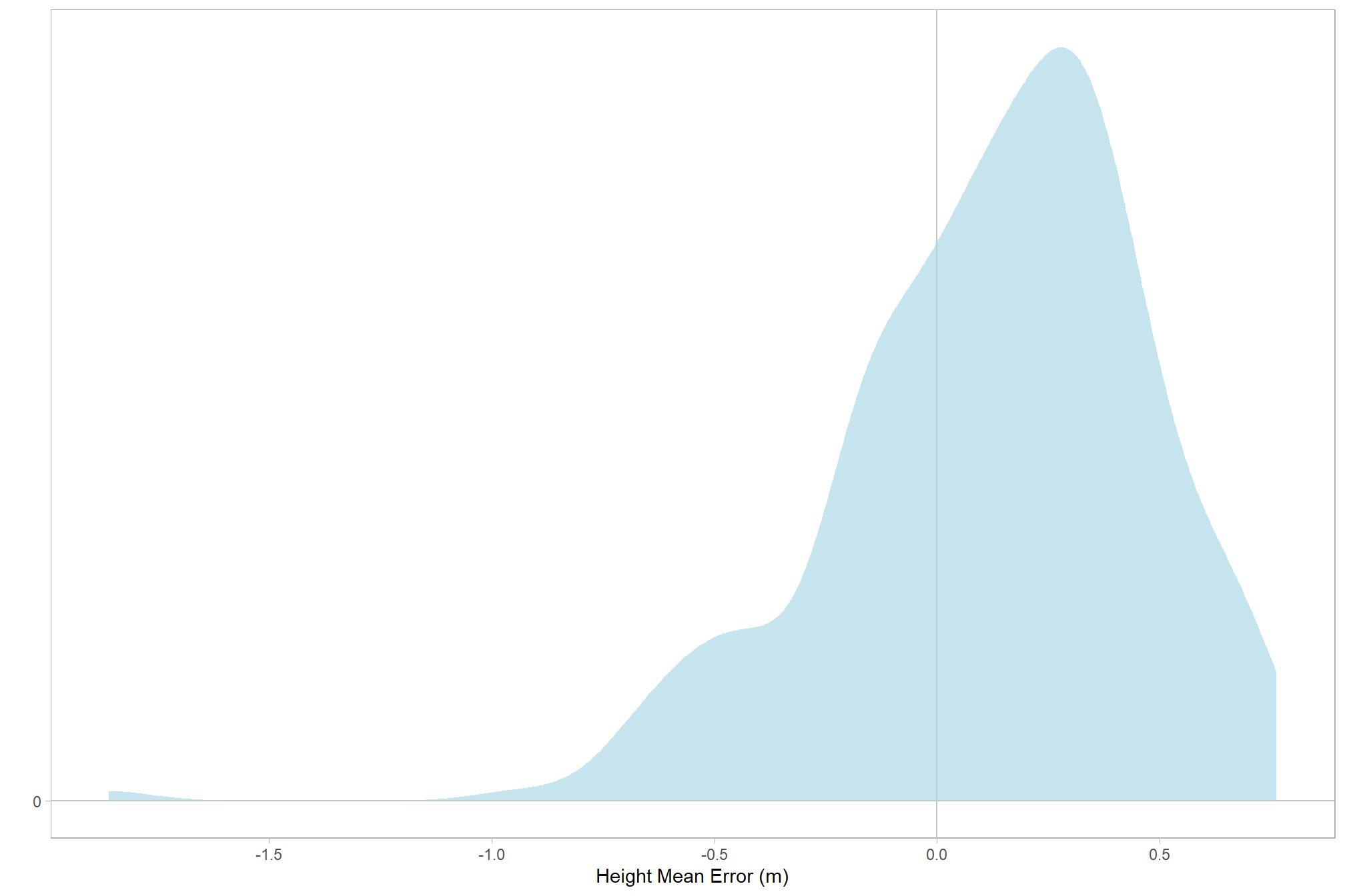
let’s check the distribution (of our dependent or \(y\) variable)
# distribution
ptcld_validation_data %>%
  ggplot(mapping = aes(x = tree_height_m_me)) +
  geom_hline(yintercept = 0, color = "gray77") +
  geom_vline(xintercept = 0, color = "gray77") +
  # geom_vline(xintercept = c(0,1)) +
  geom_density(fill = "lightblue", alpha = 0.7, color = NA) +
  labs(y="",x="Height Mean Error (m)") +
  scale_y_continuous(breaks = c(0)) +
  scale_x_continuous(breaks = scales::extended_breaks(10)) +
  theme_light() +
  theme(panel.grid = element_blank()) +
  labs(
    caption =
  )
and the summary statistics
ptcld_validation_data %>%
  dplyr::ungroup() %>%
  dplyr::select(tree_height_m_me) %>%
  dplyr::summarise(
    dplyr::across(
      dplyr::everything()
      , .fns = list(
        mean = ~ mean(.x,na.rm=T), median = ~ median(.x,na.rm=T), sd = ~ sd(.x,na.rm=T)
        , min = ~ min(.x,na.rm=T), max = ~ max(.x,na.rm=T)
        , q25 = ~ quantile(.x, 0.25, na.rm = T)
        , q75 = ~ quantile(.x, 0.75, na.rm = T)
      )
      , .names = "{.fn}"
    )
  ) %>%
  tidyr::pivot_longer(everything()) %>%
  kableExtra::kbl(caption = "summary: `tree_height_m_me`", digits = 3, col.names = NULL) %>%
kableExtra::kable_styling()| mean | 0.122 |
| median | 0.166 |
| sd | 0.355 |
| min | -1.860 |
| max | 0.763 |
| q25 | -0.088 |
| q75 | 0.356 |
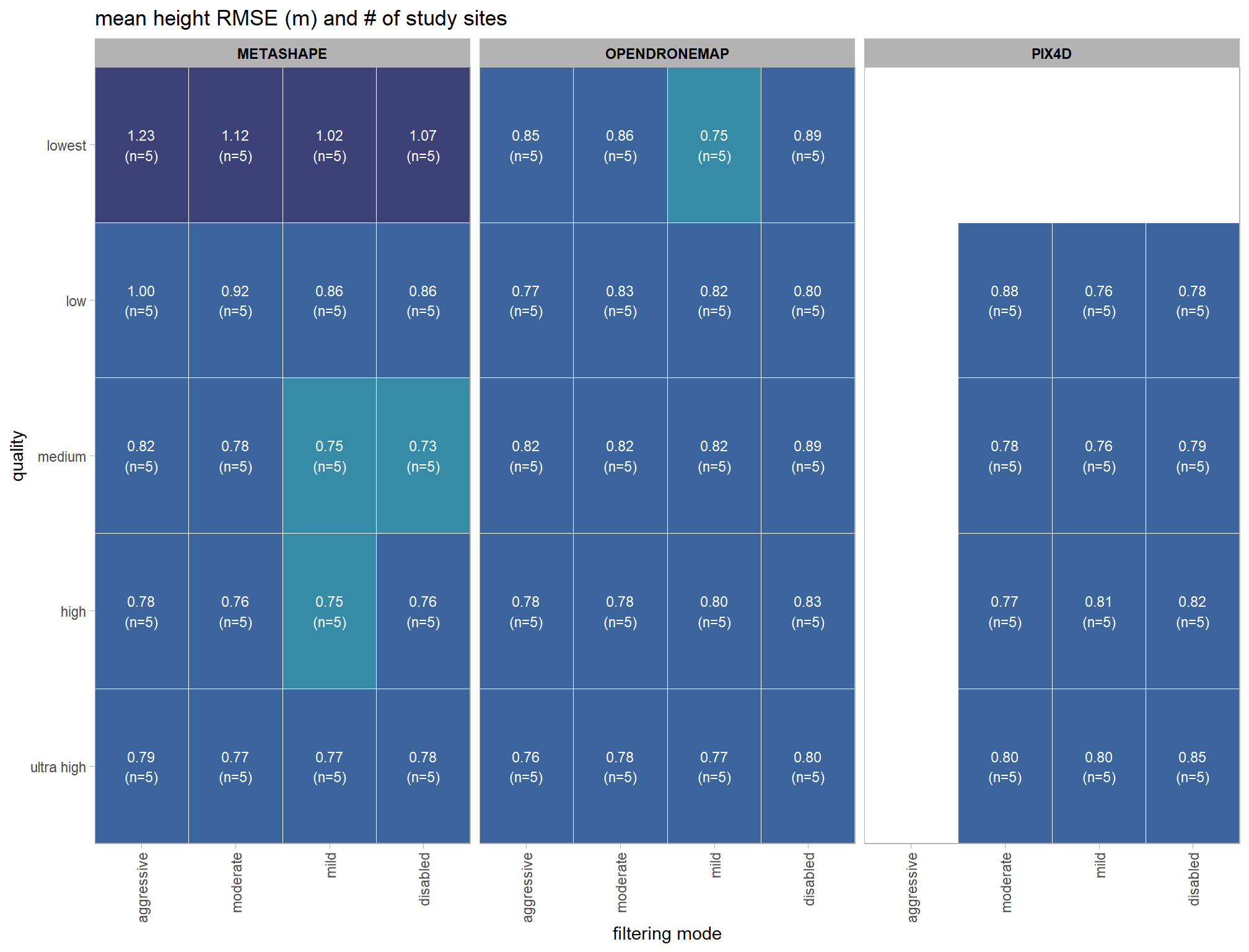
7.3.1.2 Height RMSE (precision)
  # summarize data
  dta_temp = ptcld_validation_data %>%
    dplyr::group_by(software, depth_maps_generation_quality, depth_maps_generation_filtering_mode) %>%
    # collapse across study site
    dplyr::summarise(
      tree_height_m_rmse = mean(tree_height_m_rmse, na.rm = T)
      , n = dplyr::n()
    )
  # set limits for color scale
  lmt_tree_height_m_rmse = ceiling(1.02*10*max(abs(range(dta_temp$tree_height_m_rmse, na.rm = T))))/10
  # scales::show_col(viridis::mako(n = 10, begin = 0.2, end = 0.9, direction = -1))
  # scales::show_col(scales::pal_div_gradient()(seq(0, 1, length.out = 7)))
  # plot it
  dta_temp %>%
    ggplot(mapping = aes(
      y = depth_maps_generation_quality
      , x = depth_maps_generation_filtering_mode
      , fill = tree_height_m_rmse
      , label = paste0(scales::comma(tree_height_m_rmse,accuracy = 0.01), "\n(n=", n,")")
    )) +
    geom_tile(color = "white") +
    geom_text(color = "white", size = 3) +
    facet_grid(cols = vars(software)) +
    scale_x_discrete(expand = c(0, 0)) +
    scale_y_discrete(expand = c(0, 0)) +
    scale_fill_stepsn(
      n.breaks = 5
      , colors = viridis::mako(n = 5, begin = 0.2, end = 0.9, direction = -1)
      , limits = c(0,lmt_tree_height_m_rmse)
      , labels = scales::comma_format(accuracy = 0.01)
      , show.limits = T
    ) +
    labs(
      x = "filtering mode"
      , y = "quality"
      , fill = "Height RMSE (m)"
      , title = "mean height RMSE (m) and # of study sites"
    ) +
    theme_light() +
    theme(
      legend.position = "none"
      , axis.text.x = element_text(angle = 90, vjust = 0.5, hjust = 1)
      , panel.background = element_blank()
      , panel.grid = element_blank()
      # , plot.title = element_text(hjust = 0.5)
      # , plot.subtitle = element_text(hjust = 0.5)
      , strip.text = element_text(color = "black", face = "bold")
    )
let’s check the distribution (of our dependent or \(y\) variable)
# distribution
ptcld_validation_data %>%
  ggplot(mapping = aes(x = tree_height_m_rmse)) +
  geom_hline(yintercept = 0, color = "gray77") +
  geom_vline(xintercept = 0, color = "gray77") +
  # geom_vline(xintercept = c(0,1)) +
  geom_density(fill = "lightblue", alpha = 0.7, color = NA) +
  labs(y="",x="Height RMSE (m)") +
  scale_y_continuous(breaks = c(0)) +
  scale_x_continuous(breaks = scales::extended_breaks(10)) +
  theme_light() +
  theme(panel.grid = element_blank())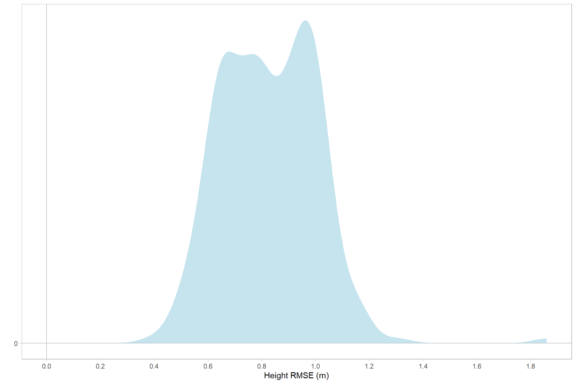
and the summary statistics
ptcld_validation_data %>%
  dplyr::ungroup() %>%
  dplyr::select(tree_height_m_rmse) %>%
  dplyr::summarise(
    dplyr::across(
      dplyr::everything()
      , .fns = list(
        mean = ~ mean(.x,na.rm=T), median = ~ median(.x,na.rm=T), sd = ~ sd(.x,na.rm=T)
        , min = ~ min(.x,na.rm=T), max = ~ max(.x,na.rm=T)
        , q25 = ~ quantile(.x, 0.25, na.rm = T)
        , q75 = ~ quantile(.x, 0.75, na.rm = T)
      )
      , .names = "{.fn}"
    )
  ) %>%
  tidyr::pivot_longer(everything()) %>%
  kableExtra::kbl(caption = "summary: `tree_height_m_rmse`", digits = 3, col.names = NULL) %>%
kableExtra::kable_styling()| mean | 0.827 |
| median | 0.819 |
| sd | 0.179 |
| min | 0.394 |
| max | 1.860 |
| q25 | 0.678 |
| q75 | 0.965 |
7.3.2 Model: Height Mean Error (bias)
# from Kurz:
gamma_a_b_from_omega_sigma = function(mode, sd) {
  if (mode <= 0) stop("mode must be > 0")
  if (sd   <= 0) stop("sd must be > 0")
  rate = (mode + sqrt(mode^2 + 4 * sd^2)) / (2 * sd^2)
  shape = 1 + mode * rate
  return(list(shape = shape, rate = rate))
}

mean_y_temp = mean(ptcld_validation_data$tree_height_m_me, na.rm = T)
sd_y_temp   = sd(ptcld_validation_data$tree_height_m_me, na.rm = T)

omega_temp = sd_y_temp / 2
sigma_temp = 2 * sd_y_temp

s_r_temp = gamma_a_b_from_omega_sigma(mode = omega_temp, sd = sigma_temp)

stanvars_temp =
  brms::stanvar(mean_y_temp,    name = "mean_y") +
  brms::stanvar(sd_y_temp,      name = "sd_y") +
  brms::stanvar(s_r_temp$shape, name = "alpha") +
  brms::stanvar(s_r_temp$rate,  name = "beta")
7.3.2.1 Prior distributions
#### setting priors
# required libraries: tidyverse, tidybayes, brms, palettetown, latex2exp
priors_temp <- c(
    brms::prior(normal(mean_y_temp, sd_y_temp * 5), class = "Intercept")
    , brms::prior(gamma(s_r_temp$shape, s_r_temp$rate), class = "sd")
    , brms::prior(cauchy(0, sd_y_temp), class = "sigma")
  )
# plot
plt_prior1 =
priors_temp %>%
  tidybayes::parse_dist() %>%
  tidybayes::marginalize_lkjcorr(K = 2) %>%
  tidyr::separate(
    .args
    , sep = ","
    , into = c("a","b")
    , remove = F
  ) %>%
  dplyr::mutate(
    distrib = paste0(
      class, " ~ "
      , .dist
      , "("
      , a %>% readr::parse_number() %>% round(2)
      , ","
      , b %>% readr::parse_number() %>% round(2)
      , ")"
    )
  ) %>%
  ggplot(., aes(dist = .dist, args = .args)) +
  facet_grid(cols=vars(distrib), scales = "free") +
  ggdist::stat_halfeye(
    aes(fill = prior),
    n = 10e2,
    show.legend = F
    , fill = "slategray"
  ) +
  coord_flip() +
  theme_light() +
  theme(
    strip.text = element_text(face = "bold", color = "black"),
    axis.text.y = element_blank(),
    axis.ticks = element_blank()
    , axis.text = element_text(size = 6)
  )+
  labs(
    x = ""
    , title = "Priors: Height Mean Error (bias)"
    , y = ""
  )
plt_prior1
7.3.2.2 Fit the model
Now fit the model.
brms_ht_me_mod = brms::brm(
  formula = tree_height_m_me ~
    # baseline
    1 +
    # main effects
    (1 | depth_maps_generation_quality) +
    (1 | depth_maps_generation_filtering_mode) +
    (1 | software) +
    (1 | study_site) + # only fitting main effects of site and not interactions
    # two-way interactions
    (1 | depth_maps_generation_quality:depth_maps_generation_filtering_mode) +
    (1 | depth_maps_generation_quality:software) +
    (1 | depth_maps_generation_filtering_mode:software) +
    # three-way interactions
    (1 | depth_maps_generation_quality:depth_maps_generation_filtering_mode:software)
  , data = ptcld_validation_data
  , family = brms::brmsfamily(family = "gaussian")
  , iter = 20000, warmup = 10000, chains = 4
  , control = list(adapt_delta = 0.999, max_treedepth = 13)
  , cores = round(parallel::detectCores()/2)
  , prior = c(
    brms::prior(normal(mean_y, sd_y * 5), class = "Intercept")
    , brms::prior(gamma(alpha, beta), class = "sd")
    , brms::prior(cauchy(0, sd_y), class = "sigma")
  )
  , stanvars = stanvars_temp
  , file = paste0(rootdir, "/fits/brms_ht_me_mod")
)
7.3.2.3 Quality:Filtering - interaction
draws_temp =
ptcld_validation_data %>%
dplyr::distinct(depth_maps_generation_quality, depth_maps_generation_filtering_mode) %>%
tidybayes::add_epred_draws(
brms_ht_me_mod, allow_new_levels = T
# this part is crucial
, re_formula = ~ (1 | depth_maps_generation_quality) +
(1 | depth_maps_generation_filtering_mode) +
(1 | depth_maps_generation_quality:depth_maps_generation_filtering_mode)
) %>%
dplyr::rename(value = .epred) %>%
dplyr::mutate(med = tidybayes::median_hdci(value)$y)
# plot
draws_temp %>%
dplyr::mutate(depth_maps_generation_quality = depth_maps_generation_quality %>% forcats::fct_rev()) %>%
# plot
ggplot(
mapping = aes(
y = value, x = depth_maps_generation_filtering_mode
, fill = med
)
) +
geom_hline(yintercept = 0, color = "gray33") +
tidybayes::stat_eye(
point_interval = median_hdi, .width = .95
, slab_alpha = 0.98
, interval_color = "black", linewidth = 1
, point_color = "black", point_fill = "black", point_size = 1
) +
scale_fill_stepsn(
n.breaks = 7
, colors = scales::pal_div_gradient()(seq(0, 1, length.out = 7))
, limits = c(-lmt_tree_height_m_me,lmt_tree_height_m_me)
, labels = scales::comma_format(accuracy = 0.1)
, show.limits = T
) +
facet_grid(cols = vars(depth_maps_generation_quality)) +
labs(
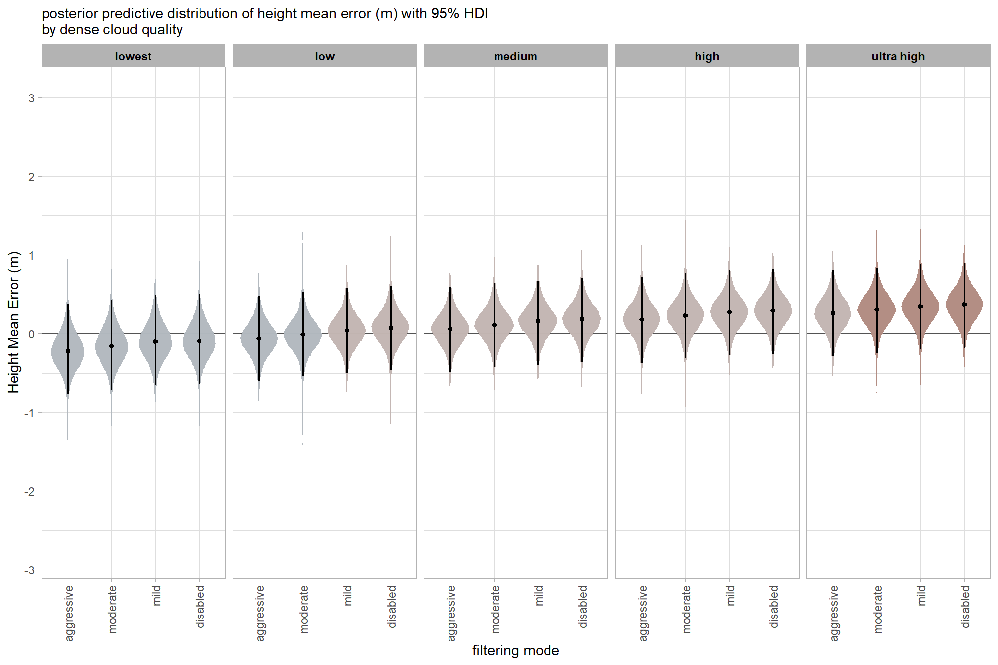
x = "filtering mode", y = "Height Mean Error (m)"
, subtitle = "posterior predictive distribution of height mean error (m) with 95% HDI\nby dense cloud quality"
) +
theme_light() +
theme(
legend.position = "none"
, legend.direction = "horizontal"
, axis.text.x = element_text(angle = 90, vjust = 0.5, hjust = 1)
, strip.text = element_text(color = "black", face = "bold")
) 
and a table of these 95% HDI values
table_temp =
  draws_temp %>%
    tidybayes::median_hdi(value) %>%
    dplyr::select(-c(.point,.interval, .width,.row)) %>%
    dplyr::arrange(depth_maps_generation_quality,depth_maps_generation_filtering_mode)

table_temp %>%
  dplyr::select(-c(depth_maps_generation_quality)) %>%
  kableExtra::kbl(
    digits = 2
    , caption = "Height Mean Error (m)<br>95% HDI of the posterior predictive distribution"
    , col.names = c(
      "filtering mode"
      , "Height Mean Error (m)<br>median"
      , "HDI low", "HDI high"
    )
    , escape = F
  ) %>%
  kableExtra::kable_styling() %>%
  kableExtra::pack_rows(index = table(forcats::fct_inorder(table_temp$depth_maps_generation_quality))) %>%
kableExtra::scroll_box(height = "8in")| filtering mode |
Height Mean Error (m) median |
HDI low | HDI high |
|---|---|---|---|
| ultra high | |||
| aggressive | 0.26 | -0.29 | 0.80 |
| moderate | 0.30 | -0.25 | 0.83 |
| mild | 0.34 | -0.20 | 0.88 |
| disabled | 0.37 | -0.18 | 0.90 |
| high | |||
| aggressive | 0.18 | -0.37 | 0.72 |
| moderate | 0.23 | -0.31 | 0.77 |
| mild | 0.27 | -0.27 | 0.81 |
| disabled | 0.29 | -0.27 | 0.82 |
| medium | |||
| aggressive | 0.06 | -0.49 | 0.59 |
| moderate | 0.11 | -0.43 | 0.64 |
| mild | 0.16 | -0.40 | 0.67 |
| disabled | 0.19 | -0.36 | 0.71 |
| low | |||
| aggressive | -0.06 | -0.61 | 0.47 |
| moderate | -0.01 | -0.54 | 0.53 |
| mild | 0.04 | -0.50 | 0.58 |
| disabled | 0.08 | -0.46 | 0.61 |
| lowest | |||
| aggressive | -0.22 | -0.78 | 0.37 |
| moderate | -0.16 | -0.72 | 0.43 |
| mild | -0.10 | -0.66 | 0.48 |
| disabled | -0.09 | -0.65 | 0.50 |
7.3.2.4 Software:Quality - interaction
draws_temp =
ptcld_validation_data %>%
dplyr::distinct(depth_maps_generation_quality, software) %>%
tidybayes::add_epred_draws(
brms_ht_me_mod, allow_new_levels = T
# this part is crucial
, re_formula = ~ (1 | depth_maps_generation_quality) +
(1 | software) +
(1 | depth_maps_generation_quality:software)
) %>%
dplyr::rename(value = .epred) %>%
dplyr::mutate(med = tidybayes::median_hdci(value)$y)
# plot
draws_temp %>%
dplyr::mutate(depth_maps_generation_quality = depth_maps_generation_quality %>% forcats::fct_rev()) %>%
# plot
ggplot(
mapping = aes(
y = value, x = software
, fill = med
)
) +
geom_hline(yintercept = 0, color = "gray33") +
tidybayes::stat_eye(
point_interval = median_hdi, .width = .95
, slab_alpha = 0.98
, interval_color = "black", linewidth = 1
, point_color = "black", point_fill = "black", point_size = 1
) +
scale_fill_stepsn(
n.breaks = 7
, colors = scales::pal_div_gradient()(seq(0, 1, length.out = 7))
, limits = c(-lmt_tree_height_m_me,lmt_tree_height_m_me)
, labels = scales::comma_format(accuracy = 0.1)
, show.limits = T
) +
facet_grid(cols = vars(depth_maps_generation_quality)) +
labs(
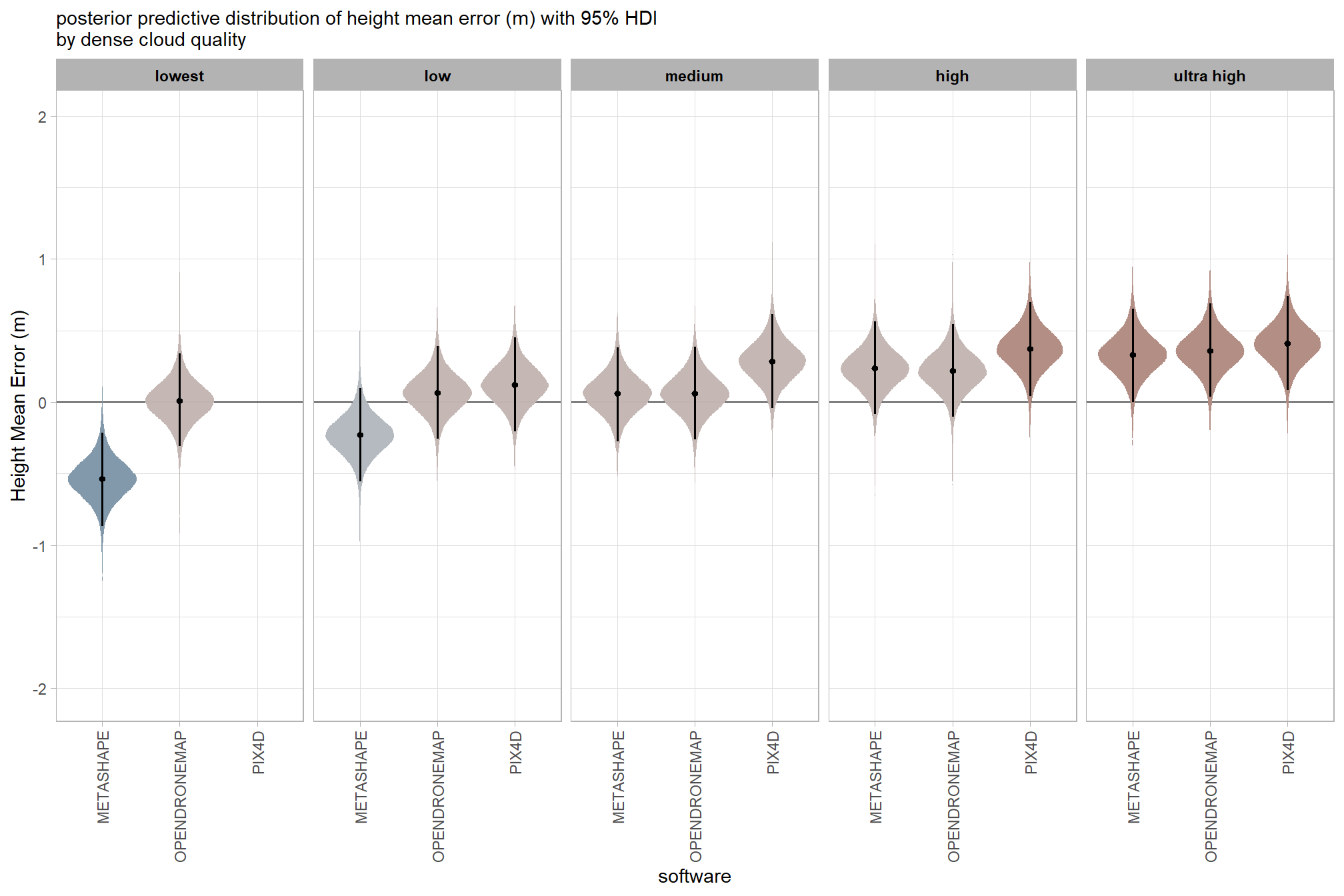
x = "software", y = "Height Mean Error (m)"
, subtitle = "posterior predictive distribution of height mean error (m) with 95% HDI\nby dense cloud quality"
) +
theme_light() +
theme(
legend.position = "none"
, legend.direction = "horizontal"
, axis.text.x = element_text(angle = 90, vjust = 0.5, hjust = 1)
, strip.text = element_text(color = "black", face = "bold")
) 
and a table of these 95% HDI values
table_temp =
  draws_temp %>%
  tidybayes::median_hdi(value) %>%
  # remove out-of-sample obs
    dplyr::inner_join(
      ptcld_validation_data %>% dplyr::distinct(depth_maps_generation_quality, software)
      , by = dplyr::join_by(depth_maps_generation_quality, software)
    ) %>%
  dplyr::select(-c(.point,.interval, .width,.row)) %>%
  dplyr::arrange(software,depth_maps_generation_quality)

table_temp %>%
  dplyr::select(-c(software)) %>%
  kableExtra::kbl(
    digits = 2
    , caption = "Height Mean Error (m)<br>95% HDI of the posterior predictive distribution"
    , col.names = c(
      "quality"
      , "Height Mean Error (m)<br>median"
      , "HDI low", "HDI high"
    )
    , escape = F
  ) %>%
  kableExtra::kable_styling() %>%
  kableExtra::pack_rows(index = table(forcats::fct_inorder(table_temp$software))) %>%
kableExtra::scroll_box(height = "8in")| quality |
Height Mean Error (m) median |
HDI low | HDI high |
|---|---|---|---|
| METASHAPE | |||
| ultra high | 0.33 | 0.00 | 0.65 |
| high | 0.24 | -0.08 | 0.57 |
| medium | 0.06 | -0.27 | 0.38 |
| low | -0.23 | -0.55 | 0.10 |
| lowest | -0.54 | -0.87 | -0.21 |
| OPENDRONEMAP | |||
| ultra high | 0.36 | 0.04 | 0.69 |
| high | 0.22 | -0.10 | 0.54 |
| medium | 0.06 | -0.26 | 0.39 |
| low | 0.07 | -0.26 | 0.39 |
| lowest | 0.01 | -0.31 | 0.34 |
| PIX4D | |||
| ultra high | 0.41 | 0.08 | 0.74 |
| high | 0.37 | 0.04 | 0.70 |
| medium | 0.29 | -0.04 | 0.61 |
| low | 0.12 | -0.21 | 0.45 |
7.3.2.5 Software:Filtering - interaction
draws_temp =
ptcld_validation_data %>%
dplyr::distinct(depth_maps_generation_filtering_mode, software) %>%
tidybayes::add_epred_draws(
brms_ht_me_mod, allow_new_levels = T
# this part is crucial
, re_formula = ~ (1 | depth_maps_generation_filtering_mode) +
(1 | software) +
(1 | depth_maps_generation_filtering_mode:software)
) %>%
dplyr::rename(value = .epred) %>%
dplyr::mutate(med = tidybayes::median_hdci(value)$y)
# plot
draws_temp %>%
# plot
ggplot(
mapping = aes(
y = value, x = software
, fill = med
)
) +
geom_hline(yintercept = 0, color = "gray33") +
tidybayes::stat_eye(
point_interval = median_hdi, .width = .95
, slab_alpha = 0.98
, interval_color = "black", linewidth = 1
, point_color = "black", point_fill = "black", point_size = 1
) +
scale_fill_stepsn(
n.breaks = 7
, colors = scales::pal_div_gradient()(seq(0, 1, length.out = 7))
, limits = c(-lmt_tree_height_m_me,lmt_tree_height_m_me)
, labels = scales::comma_format(accuracy = 0.1)
, show.limits = T
) +
facet_grid(cols = vars(depth_maps_generation_filtering_mode)) +
labs(
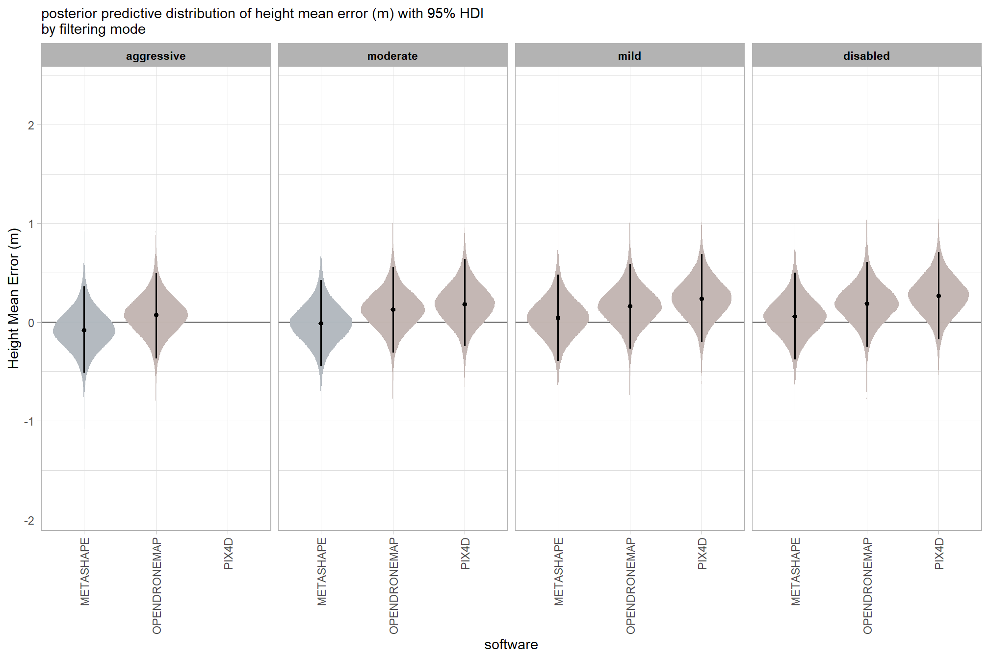
x = "software", y = "Height Mean Error (m)"
, subtitle = "posterior predictive distribution of height mean error (m) with 95% HDI\nby filtering mode"
) +
theme_light() +
theme(
legend.position = "none"
, legend.direction = "horizontal"
, axis.text.x = element_text(angle = 90, vjust = 0.5, hjust = 1)
, strip.text = element_text(color = "black", face = "bold")
) 
and a table of these 95% HDI values
table_temp =
  draws_temp %>%
    tidybayes::median_hdi(value) %>%
    dplyr::select(-c(.point,.interval, .width,.row)) %>%
    dplyr::arrange(software,depth_maps_generation_filtering_mode)

table_temp %>%
  dplyr::select(-c(software)) %>%
  kableExtra::kbl(
    digits = 2
    , caption = "Height Mean Error (m)<br>95% HDI of the posterior predictive distribution"
    , col.names = c(
      "filtering mode"
      , "Height Mean Error (m)<br>median"
      , "HDI low", "HDI high"
    )
    , escape = F
  ) %>%
  kableExtra::kable_styling() %>%
  kableExtra::pack_rows(index = table(forcats::fct_inorder(table_temp$software))) %>%
kableExtra::scroll_box(height = "8in")| filtering mode |
Height Mean Error (m) median |
HDI low | HDI high |
|---|---|---|---|
| METASHAPE | |||
| aggressive | -0.08 | -0.51 | 0.36 |
| moderate | -0.01 | -0.45 | 0.42 |
| mild | 0.04 | -0.40 | 0.48 |
| disabled | 0.06 | -0.38 | 0.50 |
| OPENDRONEMAP | |||
| aggressive | 0.07 | -0.37 | 0.49 |
| moderate | 0.13 | -0.31 | 0.55 |
| mild | 0.16 | -0.27 | 0.59 |
| disabled | 0.19 | -0.25 | 0.61 |
| PIX4D | |||
| moderate | 0.18 | -0.25 | 0.64 |
| mild | 0.24 | -0.20 | 0.69 |
| disabled | 0.27 | -0.17 | 0.71 |
7.3.2.6 Software:Quality:Filtering - interaction
# get draws
fltr_sftwr_draws_temp =
  tidyr::crossing(
    depth_maps_generation_quality = unique(ptcld_validation_data$depth_maps_generation_quality)
    , depth_maps_generation_filtering_mode = unique(ptcld_validation_data$depth_maps_generation_filtering_mode)
    , software = unique(ptcld_validation_data$software)
  ) %>%
  tidybayes::add_epred_draws(
    brms_ht_me_mod, allow_new_levels = T
    # this part is crucial
    , re_formula = ~ (1 | depth_maps_generation_quality) + # main effects
    (1 | depth_maps_generation_quality) +
    (1 | depth_maps_generation_filtering_mode) +
    (1 | software) +
    # two-way interactions
    (1 | depth_maps_generation_quality:depth_maps_generation_filtering_mode) +
    (1 | depth_maps_generation_quality:software) +
    (1 | depth_maps_generation_filtering_mode:software) +
    # three-way interactions
    (1 | depth_maps_generation_quality:depth_maps_generation_filtering_mode:software)
  ) %>%
  dplyr::rename(value = .epred) %>%
  dplyr::mutate(med = tidybayes::median_hdci(value)$y)

# plot
qlty_fltr_sftwr_ht_me =
  fltr_sftwr_draws_temp %>%
    dplyr::inner_join(
      ptcld_validation_data %>% dplyr::distinct(software, depth_maps_generation_quality, depth_maps_generation_filtering_mode)
      , by = dplyr::join_by(software, depth_maps_generation_quality, depth_maps_generation_filtering_mode)
    ) %>%
    dplyr::mutate(depth_maps_generation_quality = depth_maps_generation_quality %>% forcats::fct_rev()) %>%
    ggplot(
      mapping = aes(
        y = value
        , x = depth_maps_generation_filtering_mode
        , fill = med
      )
    ) +
    geom_hline(yintercept = 0, color = "gray33") +
    tidybayes::stat_eye(
      point_interval = median_hdi, .width = .95
      , slab_alpha = 0.98
      , interval_color = "black", linewidth = 1
      , point_color = "black", point_fill = "black", point_size = 1
    ) +
    scale_fill_stepsn(
      n.breaks = 7
      , colors = scales::pal_div_gradient()(seq(0, 1, length.out = 7))
      , limits = c(-lmt_tree_height_m_me,lmt_tree_height_m_me)
      , labels = scales::comma_format(accuracy = 0.1)
      , show.limits = T
    ) +
    facet_grid(
      rows = vars(software)
      , cols = vars(depth_maps_generation_quality)
      # , switch = "y"
    ) +
    labs(
      x = "filtering mode", y = "Height Mean Error (m)"
      , subtitle = "posterior predictive distribution of height mean error (m) with 95% HDI\nby dense cloud quality and software"
      # , caption = form_temp
    ) +
    theme_light() +
    theme(
      legend.position = "none"
      , legend.direction  = "horizontal"
      , axis.text.x = element_text(angle = 90, vjust = 0.5, hjust = 1)
      , strip.text = element_text(color = "black", face = "bold")
      , panel.grid = element_blank()
      # , strip.placement = "outside"
    ) +
    guides(
      fill = guide_legend(override.aes = list(shape = NA, size = 6, alpha = 0.9, lwd = NA))
    )
# print it
qlty_fltr_sftwr_ht_me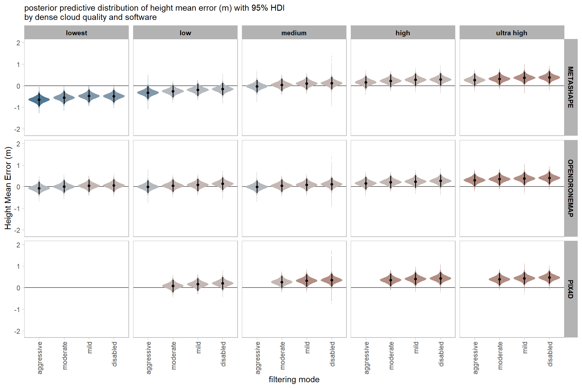
and a table of these 95% HDI values
table_temp =
  fltr_sftwr_draws_temp %>%
  tidybayes::median_hdi(value) %>%
  dplyr::inner_join(
    ptcld_validation_data %>% dplyr::distinct(software, depth_maps_generation_quality, depth_maps_generation_filtering_mode)
    , by = dplyr::join_by(software, depth_maps_generation_quality, depth_maps_generation_filtering_mode)
  ) %>%
  dplyr::mutate(depth_maps_generation_quality = depth_maps_generation_quality %>% forcats::fct_rev()) %>%
  dplyr::select(c(
    software, depth_maps_generation_quality, depth_maps_generation_filtering_mode
    , value, .lower, .upper
  )) %>%
  dplyr::ungroup() %>%
  dplyr::arrange(software, depth_maps_generation_quality, depth_maps_generation_filtering_mode)

table_temp %>%
  # dplyr::select(-c(software)) %>%
  kableExtra::kbl(
    digits = 2
    , caption = "Height Mean Error (m)<br>95% HDI of the posterior predictive distribution"
    , col.names = c(
      "software", "quality", "filtering mode"
      , "Height Mean Error (m)<br>median"
      , "HDI low", "HDI high"
    )
    , escape = F
  ) %>%
  kableExtra::kable_styling() %>%
  # kableExtra::pack_rows(index = table(forcats::fct_inorder(table_temp$software))) %>%
  kableExtra::collapse_rows(columns = 1:2, valign = "top") %>%
kableExtra::scroll_box(height = "8in")| software | quality | filtering mode |
Height Mean Error (m) median |
HDI low | HDI high |
|---|---|---|---|---|---|
| METASHAPE | lowest | aggressive | -0.65 | -0.94 | -0.36 |
| moderate | -0.55 | -0.84 | -0.27 | ||
| mild | -0.48 | -0.77 | -0.20 | ||
| disabled | -0.49 | -0.77 | -0.20 | ||
| low | aggressive | -0.32 | -0.60 | -0.03 | |
| moderate | -0.26 | -0.54 | 0.03 | ||
| mild | -0.19 | -0.48 | 0.09 | ||
| disabled | -0.16 | -0.45 | 0.13 | ||
| medium | aggressive | -0.03 | -0.32 | 0.26 | |
| moderate | 0.04 | -0.25 | 0.32 | ||
| mild | 0.10 | -0.19 | 0.38 | ||
| disabled | 0.12 | -0.16 | 0.41 | ||
| high | aggressive | 0.16 | -0.13 | 0.44 | |
| moderate | 0.22 | -0.06 | 0.51 | ||
| mild | 0.27 | -0.02 | 0.56 | ||
| disabled | 0.28 | 0.00 | 0.57 | ||
| ultra high | aggressive | 0.26 | -0.02 | 0.55 | |
| moderate | 0.32 | 0.04 | 0.61 | ||
| mild | 0.37 | 0.08 | 0.65 | ||
| disabled | 0.38 | 0.09 | 0.67 | ||
| OPENDRONEMAP | lowest | aggressive | -0.07 | -0.36 | 0.21 |
| moderate | 0.00 | -0.27 | 0.30 | ||
| mild | 0.04 | -0.24 | 0.33 | ||
| disabled | 0.05 | -0.23 | 0.33 | ||
| low | aggressive | 0.00 | -0.29 | 0.28 | |
| moderate | 0.05 | -0.24 | 0.33 | ||
| mild | 0.08 | -0.21 | 0.36 | ||
| disabled | 0.14 | -0.15 | 0.42 | ||
| medium | aggressive | -0.01 | -0.30 | 0.28 | |
| moderate | 0.04 | -0.24 | 0.33 | ||
| mild | 0.09 | -0.20 | 0.37 | ||
| disabled | 0.12 | -0.17 | 0.40 | ||
| high | aggressive | 0.16 | -0.12 | 0.45 | |
| moderate | 0.21 | -0.08 | 0.50 | ||
| mild | 0.24 | -0.05 | 0.52 | ||
| disabled | 0.27 | -0.02 | 0.55 | ||
| ultra high | aggressive | 0.30 | 0.01 | 0.58 | |
| moderate | 0.35 | 0.06 | 0.63 | ||
| mild | 0.38 | 0.09 | 0.66 | ||
| disabled | 0.41 | 0.12 | 0.69 | ||
| PIX4D | low | moderate | 0.08 | -0.21 | 0.37 |
| mild | 0.16 | -0.14 | 0.43 | ||
| disabled | 0.20 | -0.09 | 0.49 | ||
| medium | moderate | 0.26 | -0.03 | 0.55 | |
| mild | 0.32 | 0.04 | 0.61 | ||
| disabled | 0.35 | 0.06 | 0.64 | ||
| high | moderate | 0.35 | 0.07 | 0.64 | |
| mild | 0.40 | 0.13 | 0.70 | ||
| disabled | 0.43 | 0.14 | 0.72 | ||
| ultra high | moderate | 0.39 | 0.10 | 0.68 | |
| mild | 0.44 | 0.14 | 0.71 | ||
| disabled | 0.47 | 0.18 | 0.76 |
7.3.3 Model: Height RMSE (precision)
Define priors
# from Kurz:
gamma_a_b_from_omega_sigma = function(mode, sd) {
  if (mode <= 0) stop("mode must be > 0")
  if (sd   <= 0) stop("sd must be > 0")
  rate = (mode + sqrt(mode^2 + 4 * sd^2)) / (2 * sd^2)
  shape = 1 + mode * rate
  return(list(shape = shape, rate = rate))
}

mean_y_temp = mean(ptcld_validation_data$tree_height_m_rmse, na.rm = T)
sd_y_temp   = sd(ptcld_validation_data$tree_height_m_rmse, na.rm = T)

omega_temp = sd_y_temp / 2
sigma_temp = 2 * sd_y_temp

s_r_temp = gamma_a_b_from_omega_sigma(mode = omega_temp, sd = sigma_temp)

stanvars_temp =
  brms::stanvar(mean_y_temp,    name = "mean_y") +
  brms::stanvar(sd_y_temp,      name = "sd_y") +
  brms::stanvar(s_r_temp$shape, name = "alpha") +
  brms::stanvar(s_r_temp$rate,  name = "beta")
7.3.3.1 Prior distributions
#### setting priors
# required libraries: tidyverse, tidybayes, brms, palettetown, latex2exp
priors_temp <- c(
    brms::prior(normal(mean_y_temp, sd_y_temp * 5), class = "Intercept")
    , brms::prior(gamma(s_r_temp$shape, s_r_temp$rate), class = "sd")
    , brms::prior(cauchy(0, sd_y_temp), class = "sigma")
  )
# plot
plt_prior2 =
priors_temp %>%
  tidybayes::parse_dist() %>%
  tidybayes::marginalize_lkjcorr(K = 2) %>%
  tidyr::separate(
    .args
    , sep = ","
    , into = c("a","b")
    , remove = F
  ) %>%
  dplyr::mutate(
    distrib = paste0(
      class, " ~ "
      , .dist
      , "("
      , a %>% readr::parse_number() %>% round(2)
      , ","
      , b %>% readr::parse_number() %>% round(2)
      , ")"
    )
  ) %>%
  ggplot(., aes(dist = .dist, args = .args)) +
  facet_grid(cols=vars(distrib), scales = "free") +
  ggdist::stat_halfeye(
    aes(fill = prior),
    n = 10e2,
    show.legend = F
    , fill = "slategray"
  ) +
  coord_flip() +
  theme_light() +
  theme(
    strip.text = element_text(face = "bold", color = "black"),
    axis.text.y = element_blank(),
    axis.ticks = element_blank()
    , axis.text = element_text(size = 6)
  )+
  labs(
    x = ""
    , title = "Priors: Height RMSE (precision)"
    , y = ""
  )
plt_prior2
7.3.3.2 Fit the model
Now fit the model.
brms_ht_rmse_mod = brms::brm(
  formula = tree_height_m_rmse ~
    # baseline
    1 +
    # main effects
    (1 | depth_maps_generation_quality) +
    (1 | depth_maps_generation_filtering_mode) +
    (1 | software) +
    (1 | study_site) + # only fitting main effects of site and not interactions
    # two-way interactions
    (1 | depth_maps_generation_quality:depth_maps_generation_filtering_mode) +
    (1 | depth_maps_generation_quality:software) +
    (1 | depth_maps_generation_filtering_mode:software) +
    # three-way interactions
    (1 | depth_maps_generation_quality:depth_maps_generation_filtering_mode:software)
  , data = ptcld_validation_data
  , family = brms::brmsfamily(family = "gaussian")
  , iter = 20000, warmup = 10000, chains = 4
  , control = list(adapt_delta = 0.999, max_treedepth = 13)
  , cores = round(parallel::detectCores()/2)
  , prior = c(
    brms::prior(normal(mean_y, sd_y * 5), class = "Intercept")
    , brms::prior(gamma(alpha, beta), class = "sd")
    , brms::prior(cauchy(0, sd_y), class = "sigma")
  )
  , stanvars = stanvars_temp
  , file = paste0(rootdir, "/fits/brms_ht_rmse_mod")
)
7.3.3.3 Quality:Filtering - interaction
draws_temp =
  ptcld_validation_data %>%
    dplyr::distinct(depth_maps_generation_quality, depth_maps_generation_filtering_mode) %>%
    tidybayes::add_epred_draws(
      brms_ht_rmse_mod, allow_new_levels = T
      # this part is crucial
      , re_formula = ~ (1 | depth_maps_generation_quality) +
        (1 | depth_maps_generation_filtering_mode) +
        (1 | depth_maps_generation_quality:depth_maps_generation_filtering_mode)
    ) %>%
    dplyr::rename(value = .epred) %>%
    dplyr::mutate(med = tidybayes::median_hdci(value)$y)
# plot
  draws_temp %>%
    dplyr::mutate(depth_maps_generation_quality = depth_maps_generation_quality %>% forcats::fct_rev()) %>%
  # plot
  ggplot(
    mapping = aes(
      y = value, x = depth_maps_generation_filtering_mode
      , fill = med
    )
  ) +
    geom_hline(yintercept = 0, color = "gray33") +
    tidybayes::stat_eye(
      point_interval = median_hdi, .width = .95
      , slab_alpha = 0.98
      , interval_color = "black", linewidth = 1
      , point_color = "black", point_fill = "black", point_size = 1
    ) +
    scale_fill_stepsn(
      n.breaks = 5
      , colors = viridis::mako(n = 5, begin = 0.2, end = 0.9, direction = -1)
      , limits = c(0,lmt_tree_height_m_rmse)
      , labels = scales::comma_format(accuracy = 0.01)
      , show.limits = T
    ) +
    facet_grid(cols = vars(depth_maps_generation_quality)) +
    scale_y_continuous(limits = c(-0.02,NA)) +
    labs(
      x = "filtering mode", y = "Height RMSE (m)"
      , subtitle = "posterior predictive distribution of height RMSE (m) with 95% HDI\nby dense cloud quality"
    ) +
    theme_light() +
    theme(
      legend.position = "none"
      , legend.direction  = "horizontal"
      , axis.text.x = element_text(angle = 90, vjust = 0.5, hjust = 1)
      , strip.text = element_text(color = "black", face = "bold")
) 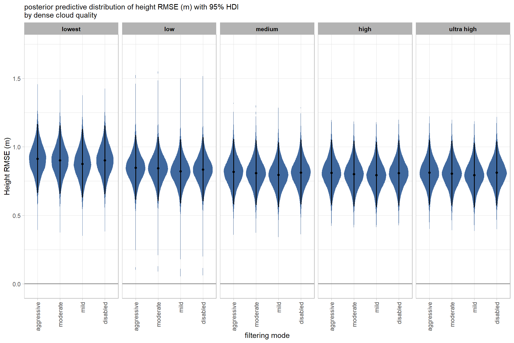
and a table of these 95% HDI values
table_temp =
  draws_temp %>%
    tidybayes::median_hdi(value) %>%
    dplyr::select(-c(.point,.interval, .width,.row)) %>%
    dplyr::arrange(depth_maps_generation_quality,depth_maps_generation_filtering_mode)

table_temp %>%
  dplyr::select(-c(depth_maps_generation_quality)) %>%
  kableExtra::kbl(
    digits = 2
    , caption = "Height RMSE (m)<br>95% HDI of the posterior predictive distribution"
    , col.names = c(
      "filtering mode"
      , "Height RMSE (m)<br>median"
      , "HDI low", "HDI high"
    )
    , escape = F
  ) %>%
  kableExtra::kable_styling() %>%
  kableExtra::pack_rows(index = table(forcats::fct_inorder(table_temp$depth_maps_generation_quality))) %>%
kableExtra::scroll_box(height = "8in")| filtering mode |
Height RMSE (m) median |
HDI low | HDI high |
|---|---|---|---|
| ultra high | |||
| aggressive | 0.81 | 0.58 | 1.05 |
| moderate | 0.81 | 0.57 | 1.04 |
| mild | 0.79 | 0.56 | 1.03 |
| disabled | 0.81 | 0.57 | 1.04 |
| high | |||
| aggressive | 0.81 | 0.57 | 1.04 |
| moderate | 0.80 | 0.57 | 1.04 |
| mild | 0.79 | 0.56 | 1.03 |
| disabled | 0.81 | 0.57 | 1.05 |
| medium | |||
| aggressive | 0.82 | 0.58 | 1.06 |
| moderate | 0.81 | 0.57 | 1.05 |
| mild | 0.80 | 0.56 | 1.03 |
| disabled | 0.81 | 0.58 | 1.05 |
| low | |||
| aggressive | 0.85 | 0.62 | 1.09 |
| moderate | 0.84 | 0.61 | 1.08 |
| mild | 0.82 | 0.59 | 1.06 |
| disabled | 0.83 | 0.60 | 1.07 |
| lowest | |||
| aggressive | 0.91 | 0.66 | 1.17 |
| moderate | 0.90 | 0.66 | 1.16 |
| mild | 0.88 | 0.63 | 1.13 |
| disabled | 0.90 | 0.66 | 1.16 |
we can also make pairwise comparisons
# first we need to define the contrasts to make
contrast_list =
  tidyr::crossing(
    x1 = unique(ptcld_validation_data$depth_maps_generation_quality)
    , x2 = unique(ptcld_validation_data$depth_maps_generation_quality)
  ) %>%
  dplyr::mutate(
    dplyr::across(
      dplyr::everything()
      , .fns = function(x){factor(
        x, ordered = T
        , levels = levels(ptcld_validation_data$depth_maps_generation_quality)
      )}
    )
  ) %>%
  dplyr::filter(x1<x2) %>%
  dplyr::arrange(x1,x2) %>%
  dplyr::mutate(dplyr::across(dplyr::everything(), as.character)) %>%
  purrr::transpose()
# make the contrasts using compare_levels
brms_contrast_temp = draws_temp %>%
    tidybayes::compare_levels(
      value
      , by = depth_maps_generation_quality
      , comparison =
        contrast_list
        # tidybayes::emmeans_comparison("revpairwise")
        #"pairwise"
    ) %>%
    dplyr::rename(contrast = depth_maps_generation_quality)

# separate contrast
brms_contrast_temp = brms_contrast_temp %>%
  dplyr::ungroup() %>%
  tidyr::separate_wider_delim(
    cols = contrast
    , delim = " - "
    , names = paste0(
        "sorter"
        , 1:(max(stringr::str_count(brms_contrast_temp$contrast, "-"))+1)
      )
    , too_few = "align_start"
    , cols_remove = F
  ) %>%
  dplyr::filter(sorter1!=sorter2) %>%
  dplyr::mutate(
    dplyr::across(
      tidyselect::starts_with("sorter")
      , .fns = function(x){factor(
        x, ordered = T
        , levels = levels(ptcld_validation_data$depth_maps_generation_quality)
      )}
    )
    , contrast = contrast %>%
      forcats::fct_reorder(
        paste0(as.numeric(sorter1), as.numeric(sorter2)) %>%
        as.numeric()
      )
    , depth_maps_generation_filtering_mode = depth_maps_generation_filtering_mode %>%
      factor(
        levels = levels(ptcld_validation_data$depth_maps_generation_filtering_mode)
        , ordered = T
      )
  ) %>%
  # median_hdi summary for coloring
  dplyr::group_by(contrast,depth_maps_generation_filtering_mode) %>%
  make_contrast_vars()

# what?
brms_contrast_temp %>% dplyr::glimpse()
## Rows: 1,600,000
## Columns: 19
## Groups: contrast, depth_maps_generation_filtering_mode [40]
## $ depth_maps_generation_filtering_mode <ord> aggressive, aggressive, aggressiv…
## $ .chain <int> NA, NA, NA, NA, NA, NA, NA, NA, N…
## $ .iteration <int> NA, NA, NA, NA, NA, NA, NA, NA, N…
## $ .draw <int> 1, 2, 3, 4, 5, 6, 7, 8, 9, 10, 11…
## $ sorter1 <ord> ultra high, ultra high, ultra hig…
## $ sorter2 <ord> high, high, high, high, high, hig…
## $ contrast <fct> ultra high - high, ultra high - h…
## $ value <dbl> 0.0077250485, -0.0013793018, -0.0…
## $ median_hdi_est <dbl> 0.001902155, 0.001902155, 0.00190…
## $ median_hdi_lower <dbl> -0.109832, -0.109832, -0.109832, …
## $ median_hdi_upper <dbl> 0.1195857, 0.1195857, 0.1195857, …
## $ pr_gt_zero <chr> "52%", "52%", "52%", "52%", "52%"…
## $ pr_lt_zero <chr> "48%", "48%", "48%", "48%", "48%"…
## $ is_diff_dir <lgl> TRUE, FALSE, FALSE, FALSE, TRUE, …
## $ pr_diff <dbl> 0.5158, 0.5158, 0.5158, 0.5158, 0…
## $ pr_diff_lab <chr> "Pr(ultra high>high)=52%", "Pr(ul…
## $ pr_diff_lab_sm <chr> "Pr(>0)=52%", "Pr(>0)=52%", "Pr(>…
## $ pr_diff_lab_pos <dbl> 0.1285546, 0.1285546, 0.1285546, …
## $ sig_level <ord> <80%, <80%, <80%, <80%, <80%, <80…plot it
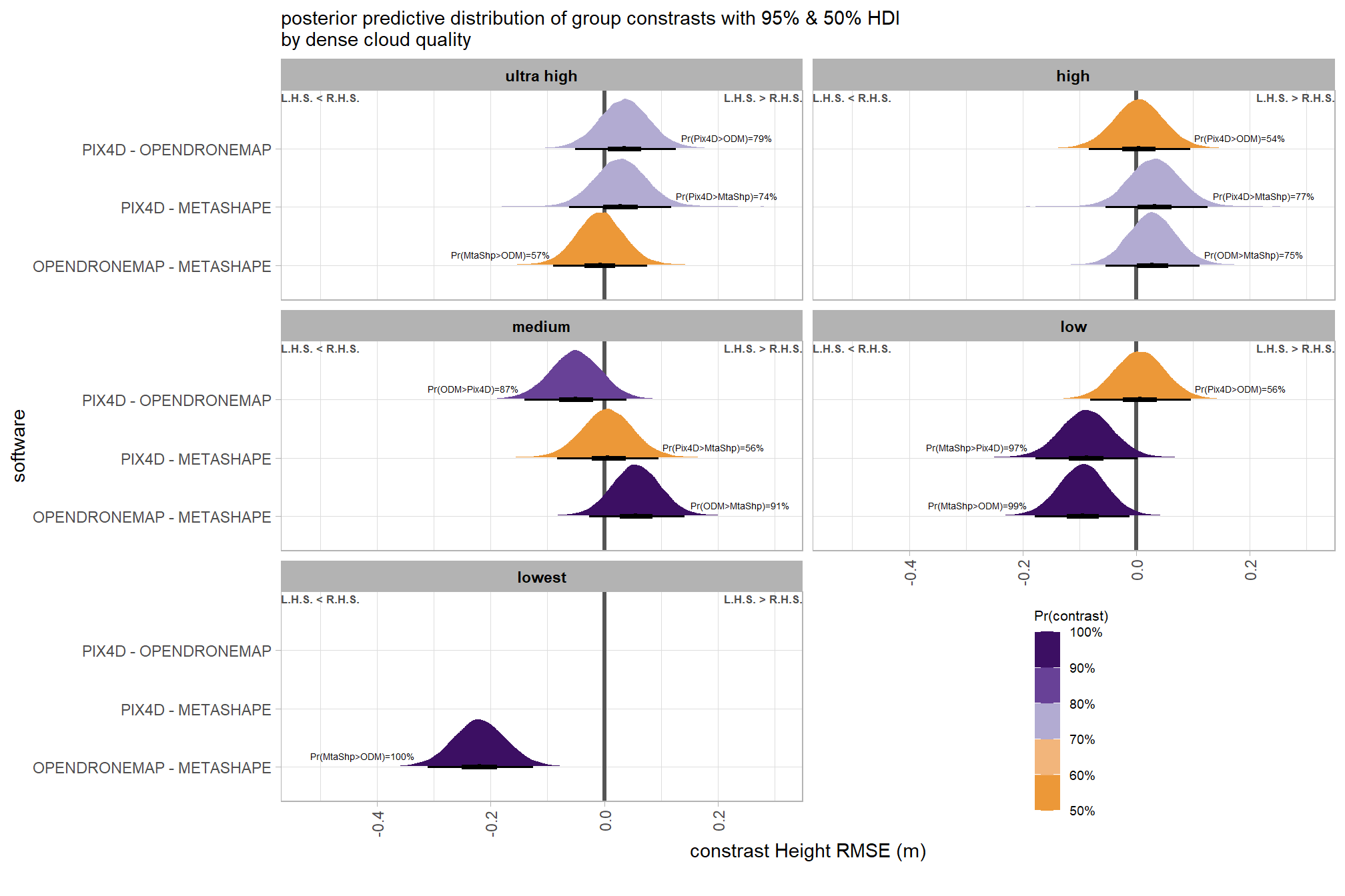
plt_contrast(
brms_contrast_temp
# , caption_text = form_temp
, y_axis_title = "quality"
, facet = "depth_maps_generation_filtering_mode"
, label_size = 1.9
, x_expand = c(1,0.95)
) +
labs(
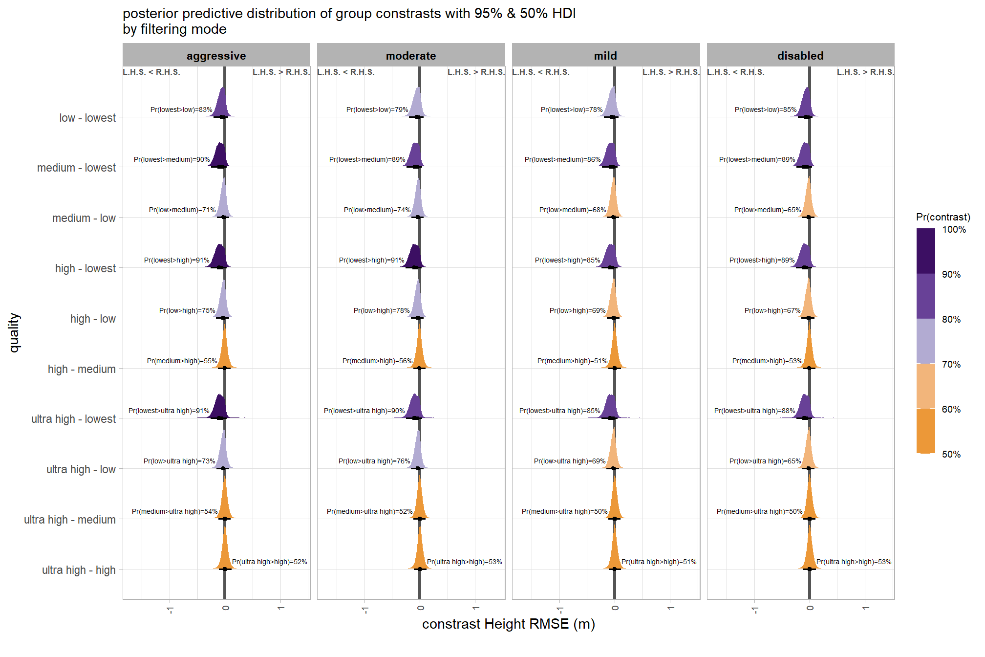
subtitle = "posterior predictive distribution of group constrasts with 95% & 50% HDI\nby filtering mode"
, x = "constrast Height RMSE (m)"
) +
theme(
axis.text.x = element_text(size = 7)
)
ggplot2::ggsave(
  "../data/qlty_fltr_comp_ht_rmse.png"
  , plot = ggplot2::last_plot() + labs(subtitle = "")
  , height = 7, width = 10.5
)
and summarize these contrasts
brms_contrast_temp %>%
  dplyr::group_by(contrast, depth_maps_generation_filtering_mode, pr_lt_zero) %>%
  tidybayes::median_hdi(value) %>%
  dplyr::arrange(contrast, depth_maps_generation_filtering_mode) %>%
  dplyr::select(contrast, depth_maps_generation_filtering_mode, value, .lower, .upper, pr_lt_zero) %>%
kableExtra::kbl(
    digits = 2
    , caption = "Height RMSE (m)<br>95% HDI of the posterior predictive distribution of group contrasts"
    , col.names = c(
      "quality contrast"
      , "filtering mode"
      , "median difference<br>Height RMSE (m)"
      , "HDI low", "HDI high"
      , "Pr(diff<0)"
    )
    , escape = F
  ) %>%
  kableExtra::kable_styling() %>%
kableExtra::scroll_box(height = "8in")| quality contrast | filtering mode |
median difference Height RMSE (m) |
HDI low | HDI high | Pr(diff<0) |
|---|---|---|---|---|---|
| ultra high - high | aggressive | 0.00 | -0.11 | 0.12 | 48% |
| ultra high - high | moderate | 0.00 | -0.11 | 0.12 | 47% |
| ultra high - high | mild | 0.00 | -0.11 | 0.11 | 49% |
| ultra high - high | disabled | 0.00 | -0.11 | 0.12 | 47% |
| ultra high - medium | aggressive | 0.00 | -0.12 | 0.11 | 54% |
| ultra high - medium | moderate | 0.00 | -0.12 | 0.11 | 52% |
| ultra high - medium | mild | 0.00 | -0.11 | 0.11 | 50% |
| ultra high - medium | disabled | 0.00 | -0.12 | 0.11 | 50% |
| ultra high - low | aggressive | -0.03 | -0.16 | 0.07 | 73% |
| ultra high - low | moderate | -0.04 | -0.16 | 0.07 | 76% |
| ultra high - low | mild | -0.02 | -0.15 | 0.08 | 69% |
| ultra high - low | disabled | -0.02 | -0.14 | 0.09 | 65% |
| ultra high - lowest | aggressive | -0.10 | -0.25 | 0.03 | 91% |
| ultra high - lowest | moderate | -0.09 | -0.25 | 0.04 | 90% |
| ultra high - lowest | mild | -0.08 | -0.23 | 0.05 | 85% |
| ultra high - lowest | disabled | -0.09 | -0.24 | 0.05 | 88% |
| high - medium | aggressive | -0.01 | -0.12 | 0.10 | 55% |
| high - medium | moderate | -0.01 | -0.12 | 0.11 | 56% |
| high - medium | mild | 0.00 | -0.11 | 0.11 | 51% |
| high - medium | disabled | 0.00 | -0.11 | 0.11 | 53% |
| high - low | aggressive | -0.03 | -0.16 | 0.07 | 75% |
| high - low | moderate | -0.04 | -0.16 | 0.07 | 78% |
| high - low | mild | -0.03 | -0.15 | 0.09 | 69% |
| high - low | disabled | -0.02 | -0.15 | 0.09 | 67% |
| high - lowest | aggressive | -0.10 | -0.26 | 0.04 | 91% |
| high - lowest | moderate | -0.10 | -0.25 | 0.04 | 91% |
| high - lowest | mild | -0.08 | -0.24 | 0.06 | 85% |
| high - lowest | disabled | -0.09 | -0.25 | 0.04 | 89% |
| medium - low | aggressive | -0.03 | -0.15 | 0.08 | 71% |
| medium - low | moderate | -0.03 | -0.15 | 0.07 | 74% |
| medium - low | mild | -0.02 | -0.14 | 0.08 | 68% |
| medium - low | disabled | -0.02 | -0.14 | 0.09 | 65% |
| medium - lowest | aggressive | -0.09 | -0.25 | 0.04 | 90% |
| medium - lowest | moderate | -0.09 | -0.24 | 0.04 | 89% |
| medium - lowest | mild | -0.08 | -0.23 | 0.06 | 86% |
| medium - lowest | disabled | -0.09 | -0.24 | 0.05 | 89% |
| low - lowest | aggressive | -0.06 | -0.21 | 0.06 | 83% |
| low - lowest | moderate | -0.05 | -0.19 | 0.07 | 79% |
| low - lowest | mild | -0.05 | -0.19 | 0.07 | 78% |
| low - lowest | disabled | -0.06 | -0.21 | 0.05 | 85% |
7.3.3.4 Software:Quality - interaction
draws_temp =
tidyr::crossing(
depth_maps_generation_quality = unique(ptcld_validation_data$depth_maps_generation_quality)
, software = unique(ptcld_validation_data$software)
) %>%
tidybayes::add_epred_draws(
brms_ht_rmse_mod, allow_new_levels = T
# this part is crucial
, re_formula = ~ (1 | depth_maps_generation_quality) +
(1 | software) +
(1 | depth_maps_generation_quality:software)
) %>%
dplyr::rename(value = .epred) %>%
dplyr::mutate(med = tidybayes::median_hdci(value)$y)
# plot
draws_temp %>%
# remove out-of-sample obs
dplyr::inner_join(
ptcld_validation_data %>% dplyr::distinct(depth_maps_generation_quality, software)
, by = dplyr::join_by(depth_maps_generation_quality, software)
) %>%
dplyr::mutate(depth_maps_generation_quality = depth_maps_generation_quality %>% forcats::fct_rev()) %>%
# plot
ggplot(
mapping = aes(
y = value, x = software
, fill = med
)
) +
geom_hline(yintercept = 0, color = "gray33") +
tidybayes::stat_eye(
point_interval = median_hdi, .width = .95
, slab_alpha = 0.98
, interval_color = "black", linewidth = 1
, point_color = "black", point_fill = "black", point_size = 1
) +
scale_fill_stepsn(
n.breaks = 5
, colors = viridis::mako(n = 5, begin = 0.2, end = 0.9, direction = -1)
, limits = c(0,lmt_tree_height_m_rmse)
, labels = scales::comma_format(accuracy = 0.01)
, show.limits = T
) +
facet_grid(cols = vars(depth_maps_generation_quality)) +
scale_y_continuous(limits = c(-0.02,NA)) +
labs(
x = "software", y = "Height RMSE (m)"
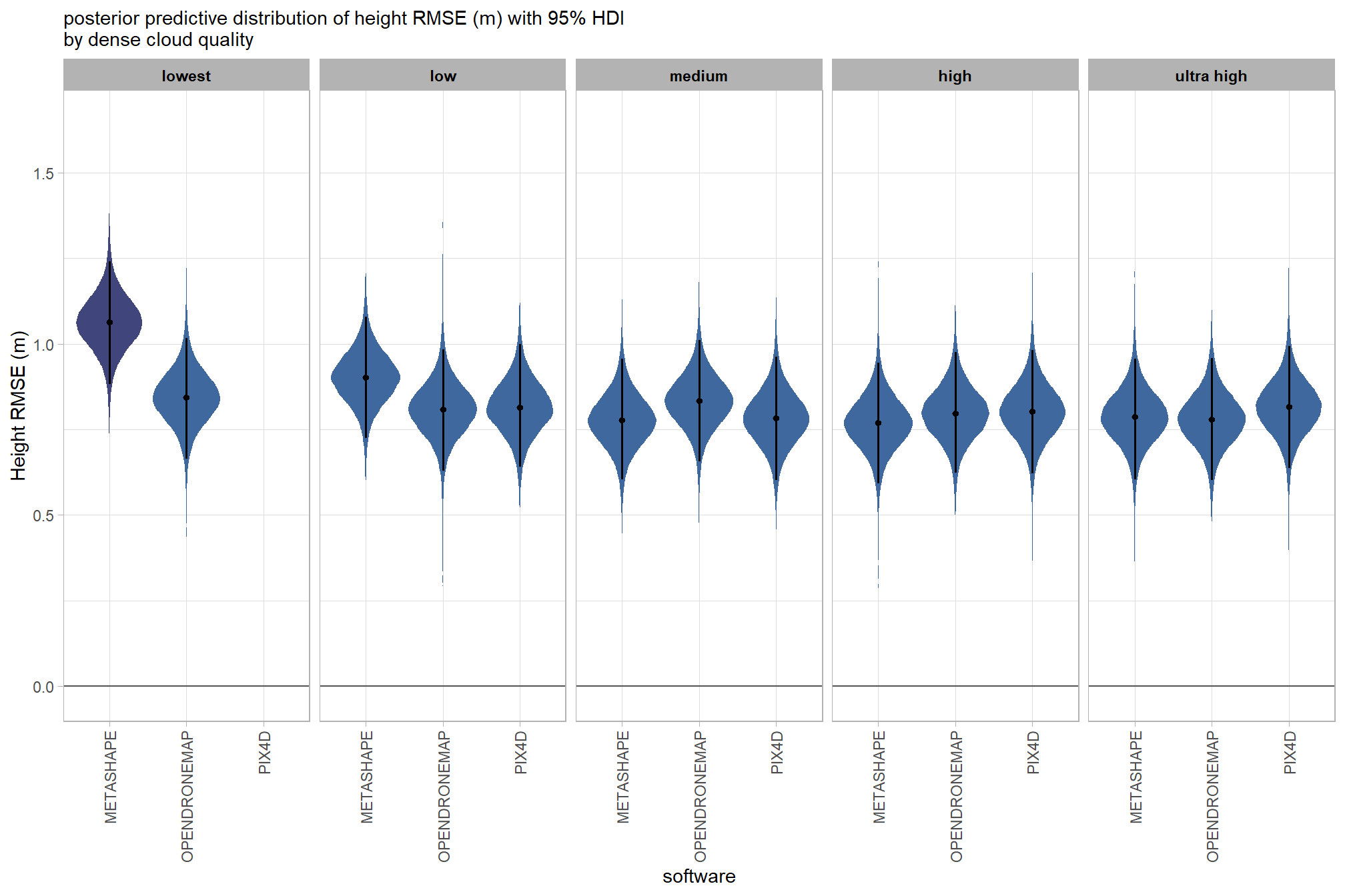
, subtitle = "posterior predictive distribution of height RMSE (m) with 95% HDI\nby dense cloud quality"
) +
theme_light() +
theme(
legend.position = "none"
, legend.direction = "horizontal"
, axis.text.x = element_text(angle = 90, vjust = 0.5, hjust = 1)
, strip.text = element_text(color = "black", face = "bold")
) 
and a table of these 95% HDI values
table_temp =
  draws_temp %>%
  tidybayes::median_hdi(value) %>%
  # remove out-of-sample obs
    dplyr::inner_join(
      ptcld_validation_data %>% dplyr::distinct(depth_maps_generation_quality, software)
      , by = dplyr::join_by(depth_maps_generation_quality, software)
    ) %>%
  dplyr::select(-c(.point,.interval, .width,.row)) %>%
  dplyr::arrange(software,depth_maps_generation_quality)

table_temp %>%
  dplyr::select(-c(software)) %>%
  kableExtra::kbl(
    digits = 2
    , caption = "Height RMSE (m)<br>95% HDI of the posterior predictive distribution"
    , col.names = c(
      "quality"
      , "Height RMSE (m)<br>median"
      , "HDI low", "HDI high"
    )
    , escape = F
  ) %>%
  kableExtra::kable_styling() %>%
  kableExtra::pack_rows(index = table(forcats::fct_inorder(table_temp$software))) %>%
kableExtra::scroll_box(height = "8in")| quality |
Height RMSE (m) median |
HDI low | HDI high |
|---|---|---|---|
| METASHAPE | |||
| ultra high | 0.79 | 0.60 | 0.96 |
| high | 0.77 | 0.59 | 0.94 |
| medium | 0.78 | 0.60 | 0.96 |
| low | 0.90 | 0.73 | 1.08 |
| lowest | 1.06 | 0.88 | 1.24 |
| OPENDRONEMAP | |||
| ultra high | 0.78 | 0.60 | 0.96 |
| high | 0.80 | 0.62 | 0.97 |
| medium | 0.83 | 0.66 | 1.01 |
| low | 0.81 | 0.63 | 0.98 |
| lowest | 0.84 | 0.66 | 1.02 |
| PIX4D | |||
| ultra high | 0.82 | 0.64 | 0.99 |
| high | 0.80 | 0.62 | 0.98 |
| medium | 0.78 | 0.60 | 0.96 |
| low | 0.81 | 0.64 | 1.00 |
we can also make pairwise comparisons
# calculate contrast
brms_contrast_temp = draws_temp %>%
  tidybayes::compare_levels(
    value
    , by = depth_maps_generation_quality
    , comparison = contrast_list
  ) %>%
  dplyr::rename(contrast = depth_maps_generation_quality)

# separate contrast
brms_contrast_temp = brms_contrast_temp %>%
  dplyr::ungroup() %>%
  tidyr::separate_wider_delim(
    cols = contrast
    , delim = " - "
    , names = paste0(
      "sorter"
      , 1:(max(stringr::str_count(brms_contrast_temp$contrast, "-"))+1)
    )
    , too_few = "align_start"
    , cols_remove = F
  ) %>%
  dplyr::filter(sorter1!=sorter2) %>%
  dplyr::mutate(
    dplyr::across(
      tidyselect::starts_with("sorter")
      , .fns = function(x){factor(
        x, ordered = T
        , levels = levels(ptcld_validation_data$depth_maps_generation_quality)
      )}
    )
    , contrast = contrast %>%
      forcats::fct_reorder(
        paste0(as.numeric(sorter1), as.numeric(sorter2)) %>%
          as.numeric()
      )
  ) %>%
  # median_hdi summary for coloring
  dplyr::group_by(contrast, software) %>%
  make_contrast_vars()

# remove out-of-sample obs
brms_contrast_temp = brms_contrast_temp %>%
  dplyr::inner_join(
    ptcld_validation_data %>% dplyr::distinct(software, depth_maps_generation_quality)
    , by = dplyr::join_by(software, sorter1 == depth_maps_generation_quality)
  ) %>%
  dplyr::inner_join(
    ptcld_validation_data %>% dplyr::distinct(software, depth_maps_generation_quality)
    , by = dplyr::join_by(software, sorter2 == depth_maps_generation_quality)
  )
plot it
plt_contrast(
brms_contrast_temp
# , caption_text = form_temp
, y_axis_title = "quality"
, facet = "software"
, label_size = 1.9
, x_expand = c(0.83,0.82)
) +
labs(
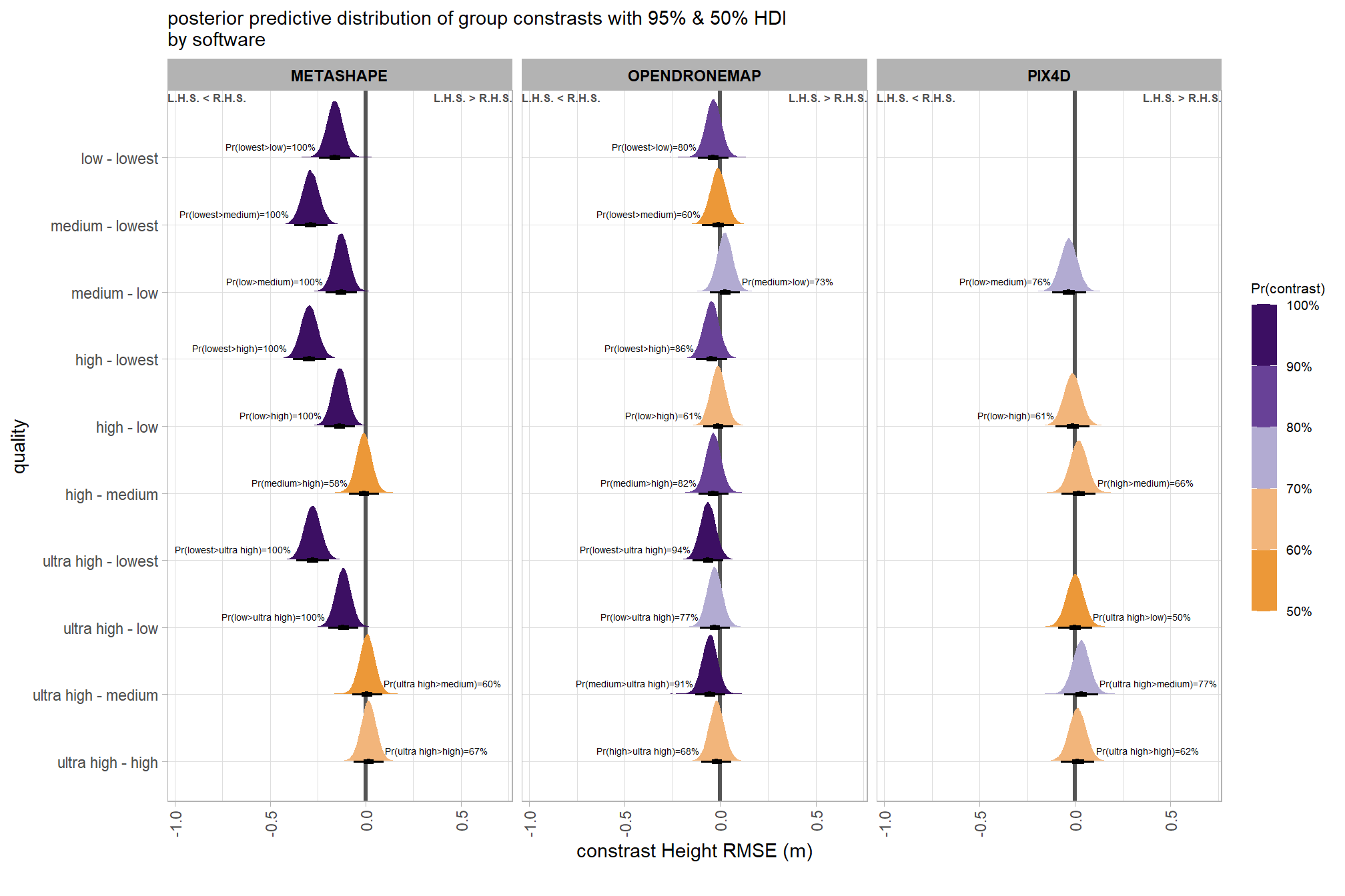
subtitle = "posterior predictive distribution of group constrasts with 95% & 50% HDI\nby software"
, x = "constrast Height RMSE (m)"
)
ggplot2::ggsave(
  "../data/qlty_sftwr_comp_ht_rmse.png"
  , plot = ggplot2::last_plot() + labs(subtitle = "")
  , height = 7, width = 10.5
)
create plot for combining with other RMSE contrasts for publication
ptchwrk_qlty_sftwr_comp_ht_rmse =
  plt_contrast(
    brms_contrast_temp
    , y_axis_title = "quality contrast"
    , facet = "software"
    , label_size = 1.5
    , label = "pr_diff_lab_sm"
    , annotate_size = 1.6
  ) +
    labs(
      subtitle = "" # "constrast Height RMSE (m)"
      , x = "Height RMSE (m) constrast"
    ) +
    theme(
      legend.position="none"
      , axis.title.y = element_text(size = 10, face = "bold")
      , axis.title.x = element_text(size = 8)
    )
# ptchwrk_qlty_sftwr_comp_ht_rmse
and summarize these contrasts
table_temp = brms_contrast_temp %>%
  dplyr::group_by(contrast, software, pr_lt_zero) %>%
  tidybayes::median_hdi(value) %>%
  dplyr::arrange(contrast, software) %>%
  dplyr::select(contrast, software, value, .lower, .upper, pr_lt_zero) %>%
  dplyr::arrange(software, contrast)

table_temp %>%
  dplyr::select(-c(software)) %>%
  kableExtra::kbl(
    digits = 2
    , caption = "Height RMSE (m)<br>95% HDI of the posterior predictive distribution of group contrasts"
    , col.names = c(
      "quality contrast"
      , "median difference<br>Height RMSE (m)"
      , "HDI low", "HDI high"
      , "Pr(diff<0)"
    )
    , escape = F
  ) %>%
  kableExtra::kable_styling() %>%
  kableExtra::pack_rows(index = table(forcats::fct_inorder(table_temp$software))) %>%
kableExtra::scroll_box(height = "8in")| quality contrast |
median difference Height RMSE (m) |
HDI low | HDI high | Pr(diff<0) |
|---|---|---|---|---|
| METASHAPE | ||||
| ultra high - high | 0.02 | -0.06 | 0.10 | 33% |
| ultra high - medium | 0.01 | -0.07 | 0.09 | 40% |
| ultra high - low | -0.12 | -0.20 | -0.04 | 100% |
| ultra high - lowest | -0.28 | -0.36 | -0.19 | 100% |
| high - medium | -0.01 | -0.09 | 0.07 | 58% |
| high - low | -0.13 | -0.21 | -0.05 | 100% |
| high - lowest | -0.29 | -0.38 | -0.21 | 100% |
| medium - low | -0.13 | -0.21 | -0.05 | 100% |
| medium - lowest | -0.29 | -0.37 | -0.20 | 100% |
| low - lowest | -0.16 | -0.24 | -0.08 | 100% |
| OPENDRONEMAP | ||||
| ultra high - high | -0.02 | -0.10 | 0.06 | 68% |
| ultra high - medium | -0.05 | -0.13 | 0.03 | 91% |
| ultra high - low | -0.03 | -0.11 | 0.05 | 77% |
| ultra high - lowest | -0.06 | -0.15 | 0.02 | 94% |
| high - medium | -0.04 | -0.11 | 0.04 | 82% |
| high - low | -0.01 | -0.09 | 0.07 | 61% |
| high - lowest | -0.05 | -0.13 | 0.04 | 86% |
| medium - low | 0.02 | -0.05 | 0.10 | 27% |
| medium - lowest | -0.01 | -0.10 | 0.07 | 60% |
| low - lowest | -0.04 | -0.12 | 0.04 | 80% |
| PIX4D | ||||
| ultra high - high | 0.01 | -0.08 | 0.10 | 38% |
| ultra high - medium | 0.03 | -0.06 | 0.12 | 23% |
| ultra high - low | 0.00 | -0.09 | 0.09 | 50% |
| high - medium | 0.02 | -0.07 | 0.11 | 34% |
| high - low | -0.01 | -0.10 | 0.08 | 61% |
| medium - low | -0.03 | -0.12 | 0.06 | 76% |
The contrasts above address the question “are there differences in RMSE based on dense point cloud generation quality within each software?”.
To address the different question of “are there differences in RMSE based on the processing software used at a given dense point cloud generation quality?” we need to utilize a different formulation of the comparison parameter within our call to the tidybayes::compare_levels function and calculate the contrast by software instead
# calculate contrast
brms_contrast_temp = draws_temp %>%
  tidybayes::compare_levels(
    value
    , by = software
    , comparison = "pairwise"
  ) %>%
  dplyr::rename(contrast = software) %>%
  # median_hdi summary for coloring
  dplyr::group_by(contrast, depth_maps_generation_quality) %>%
  make_contrast_vars()

# remove out-of-sample obs
brms_contrast_temp = brms_contrast_temp %>%
  tidyr::separate_wider_delim(
    cols = contrast
    , delim = " - "
    , names = paste0(
      "sorter"
      , 1:(max(stringr::str_count(brms_contrast_temp$contrast, "-"))+1)
    )
    , too_few = "align_start"
    , cols_remove = F
  ) %>%
  dplyr::filter(sorter1!=sorter2) %>%
  dplyr::inner_join(
    ptcld_validation_data %>% dplyr::distinct(software, depth_maps_generation_quality)
    , by = dplyr::join_by(sorter1 == software, depth_maps_generation_quality)
  ) %>%
  dplyr::inner_join(
    ptcld_validation_data %>% dplyr::distinct(software, depth_maps_generation_quality)
    , by = dplyr::join_by(sorter2 == software, depth_maps_generation_quality)
  )
plot it
plt_contrast(
  brms_contrast_temp
  # , caption_text = form_temp
  , y_axis_title = "software"
  , facet = "depth_maps_generation_quality"
  , label_size = 1.9
  , x_expand = c(0.25,0.1)
) +
  facet_wrap(facets = vars(depth_maps_generation_quality), ncol = 2) +
  labs(
    subtitle = "posterior predictive distribution of group constrasts with 95% & 50% HDI\nby dense cloud quality"
    , x = "constrast Height RMSE (m)"
  ) +
  theme(
    legend.position = c(.75, .13)
  ) +
  guides(fill = guide_colorbar(theme = theme(
    legend.key.width  = unit(1, "lines"),
    legend.key.height = unit(7, "lines")
  )))
ggplot2::ggsave(
  "../data/sftwr_qlty_comp_ht_rmse.png"
  , plot = ggplot2::last_plot() + labs(subtitle = "")
  , height = 7, width = 10.5
)
create plot for combining with other RMSE contrasts for publication
ptchwrk_sftwr_qlty_comp_ht_rmse =
  plt_contrast(
    brms_contrast_temp
    , y_axis_title = "software contrast"
    , facet = "depth_maps_generation_quality"
    , label_size = 1.7
    , label = "pr_diff_lab_sm"
    , annotate_size = 1.8
  ) +
    facet_wrap(facets = vars(depth_maps_generation_quality), ncol = 3) +
    labs(
      subtitle = ""
      , x = "Height RMSE (m) constrast"
    ) +
    theme(
      legend.position = "inside"
      , legend.position.inside = c(.8, .10)
      , axis.title.y = element_text(size = 10, face = "bold")
      , axis.title.x = element_text(size = 8)
    ) +
    guides(fill = guide_colorbar(theme = theme(
      legend.key.width  = unit(1, "lines"),
      legend.key.height = unit(6.5, "lines")
    )))
# ptchwrk_sftwr_qlty_comp_ht_rmse
and summarize these contrasts
table_temp = brms_contrast_temp %>%
  dplyr::group_by(contrast, depth_maps_generation_quality, pr_lt_zero) %>%
  tidybayes::median_hdi(value) %>%
  dplyr::arrange(contrast, depth_maps_generation_quality) %>%
  dplyr::select(contrast, depth_maps_generation_quality, value, .lower, .upper, pr_lt_zero)

table_temp %>%
  dplyr::select(-c(contrast)) %>%
  kableExtra::kbl(
    digits = 2
    , caption = "Height RMSE (m)<br>95% HDI of the posterior predictive distribution of group contrasts"
    , col.names = c(
      "quality"
      , "median difference<br>Height RMSE (m)"
      , "HDI low", "HDI high"
      , "Pr(diff<0)"
    )
    , escape = F
  ) %>%
  kableExtra::kable_styling() %>%
  kableExtra::pack_rows(index = table(forcats::fct_inorder(table_temp$contrast))) %>%
kableExtra::scroll_box(height = "8in")| quality |
median difference Height RMSE (m) |
HDI low | HDI high | Pr(diff<0) |
|---|---|---|---|---|
| OPENDRONEMAP - METASHAPE | ||||
| ultra high | -0.01 | -0.09 | 0.08 | 57% |
| high | 0.03 | -0.05 | 0.11 | 25% |
| medium | 0.06 | -0.03 | 0.14 | 9% |
| low | -0.09 | -0.18 | -0.01 | 99% |
| lowest | -0.22 | -0.31 | -0.13 | 100% |
| PIX4D - METASHAPE | ||||
| ultra high | 0.03 | -0.06 | 0.12 | 26% |
| high | 0.03 | -0.05 | 0.13 | 23% |
| medium | 0.01 | -0.08 | 0.10 | 44% |
| low | -0.09 | -0.18 | 0.00 | 97% |
| PIX4D - OPENDRONEMAP | ||||
| ultra high | 0.04 | -0.05 | 0.13 | 21% |
| high | 0.00 | -0.08 | 0.10 | 46% |
| medium | -0.05 | -0.14 | 0.04 | 87% |
| low | 0.01 | -0.08 | 0.10 | 44% |
7.3.3.5 Software:Filtering - interaction
draws_temp =
tidyr::crossing(
depth_maps_generation_filtering_mode = unique(ptcld_validation_data$depth_maps_generation_filtering_mode)
, software = unique(ptcld_validation_data$software)
) %>%
tidybayes::add_epred_draws(
brms_ht_rmse_mod, allow_new_levels = T
# this part is crucial
, re_formula = ~ (1 | depth_maps_generation_filtering_mode) +
(1 | software) +
(1 | depth_maps_generation_filtering_mode:software)
) %>%
dplyr::rename(value = .epred) %>%
dplyr::mutate(med = tidybayes::median_hdci(value)$y)
# plot
draws_temp %>%
# remove out-of-sample obs
dplyr::inner_join(
ptcld_validation_data %>% dplyr::distinct(depth_maps_generation_filtering_mode, software)
, by = dplyr::join_by(depth_maps_generation_filtering_mode, software)
) %>%
# plot
ggplot(
mapping = aes(
y = value, x = software
, fill = med
)
) +
geom_hline(yintercept = 0, color = "gray33") +
tidybayes::stat_eye(
point_interval = median_hdi, .width = .95
, slab_alpha = 0.98
, interval_color = "black", linewidth = 1
, point_color = "black", point_fill = "black", point_size = 1
) +
scale_fill_stepsn(
n.breaks = 5
, colors = viridis::mako(n = 5, begin = 0.2, end = 0.9, direction = -1)
, limits = c(0,lmt_tree_height_m_rmse)
, labels = scales::comma_format(accuracy = 0.01)
, show.limits = T
) +
facet_grid(cols = vars(depth_maps_generation_filtering_mode)) +
scale_y_continuous(limits = c(-0.02,NA)) +
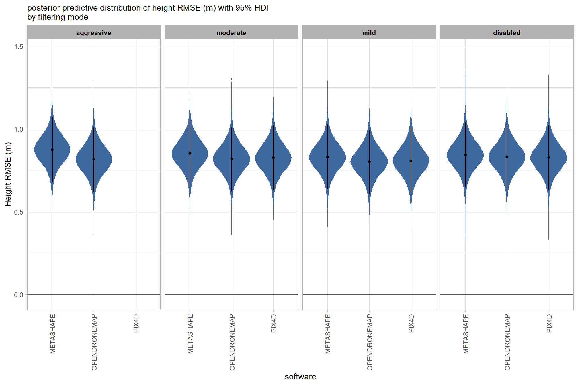
labs(
x = "software", y = "Height RMSE (m)"
, subtitle = "posterior predictive distribution of height RMSE (m) with 95% HDI\nby filtering mode"
) +
theme_light() +
theme(
legend.position = "none"
, legend.direction = "horizontal"
, axis.text.x = element_text(angle = 90, vjust = 0.5, hjust = 1)
, strip.text = element_text(color = "black", face = "bold")
) 
and a table of these 95% HDI values
table_temp =
  draws_temp %>%
    tidybayes::median_hdi(value) %>%
    dplyr::select(-c(.point,.interval, .width,.row)) %>%
    dplyr::arrange(software,depth_maps_generation_filtering_mode)

table_temp %>%
  dplyr::select(-c(software)) %>%
  kableExtra::kbl(
    digits = 2
    , caption = "Height RMSE (m)<br>95% HDI of the posterior predictive distribution"
    , col.names = c(
      "filtering mode"
      , "Height RMSE (m)<br>median"
      , "HDI low", "HDI high"
    )
    , escape = F
  ) %>%
  kableExtra::kable_styling() %>%
  kableExtra::pack_rows(index = table(forcats::fct_inorder(table_temp$software))) %>%
kableExtra::scroll_box(height = "8in")| filtering mode |
Height RMSE (m) median |
HDI low | HDI high |
|---|---|---|---|
| METASHAPE | |||
| aggressive | 0.88 | 0.68 | 1.07 |
| moderate | 0.85 | 0.66 | 1.05 |
| mild | 0.83 | 0.64 | 1.03 |
| disabled | 0.84 | 0.65 | 1.04 |
| OPENDRONEMAP | |||
| aggressive | 0.82 | 0.62 | 1.01 |
| moderate | 0.82 | 0.62 | 1.01 |
| mild | 0.80 | 0.61 | 0.99 |
| disabled | 0.83 | 0.64 | 1.02 |
| PIX4D | |||
| aggressive | 0.83 | 0.63 | 1.04 |
| moderate | 0.83 | 0.63 | 1.02 |
| mild | 0.81 | 0.61 | 1.01 |
| disabled | 0.83 | 0.63 | 1.02 |
we can also make pairwise comparisons
# calculate contrast
brms_contrast_temp = draws_temp %>%
  tidybayes::compare_levels(
    value
    , by = depth_maps_generation_filtering_mode
    , comparison = "pairwise"
  ) %>%
  dplyr::rename(contrast = depth_maps_generation_filtering_mode)

# separate contrast
brms_contrast_temp = brms_contrast_temp %>%
  dplyr::ungroup() %>%
  tidyr::separate_wider_delim(
    cols = contrast
    , delim = " - "
    , names = paste0(
      "sorter"
      , 1:(max(stringr::str_count(brms_contrast_temp$contrast, "-"))+1)
    )
    , too_few = "align_start"
    , cols_remove = F
  ) %>%
  dplyr::filter(sorter1!=sorter2) %>%
  dplyr::mutate(
    dplyr::across(
      tidyselect::starts_with("sorter")
      , .fns = function(x){factor(
        x, ordered = T
        , levels = levels(ptcld_validation_data$depth_maps_generation_filtering_mode)
      )}
    )
    , contrast = contrast %>%
      forcats::fct_reorder(
        paste0(as.numeric(sorter1), as.numeric(sorter2)) %>%
          as.numeric()
      ) %>%
      # re order for filtering mode
      forcats::fct_rev()
  ) %>%
  # median_hdi summary for coloring
  dplyr::group_by(contrast, software) %>%
  make_contrast_vars()

# remove out-of-sample obs
brms_contrast_temp = brms_contrast_temp %>%
  dplyr::inner_join(
    ptcld_validation_data %>% dplyr::distinct(software, depth_maps_generation_filtering_mode)
    , by = dplyr::join_by(software, sorter1 == depth_maps_generation_filtering_mode)
  ) %>%
  dplyr::inner_join(
    ptcld_validation_data %>% dplyr::distinct(software, depth_maps_generation_filtering_mode)
    , by = dplyr::join_by(software, sorter2 == depth_maps_generation_filtering_mode)
  )
plot it
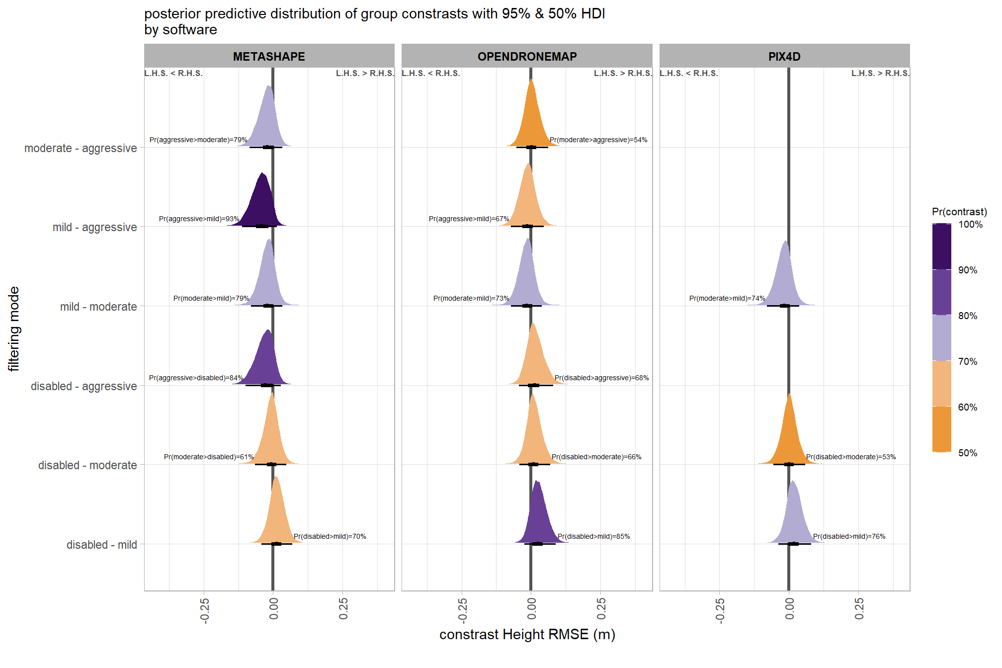
plt_contrast(
  brms_contrast_temp
  # , caption_text = form_temp
  , y_axis_title = "filtering mode"
  , facet = "software"
  , label_size = 1.9
  , x_expand = c(0.6,0.45)
) +
  labs(
    subtitle = "posterior predictive distribution of group constrasts with 95% & 50% HDI\nby software"
    , x = "constrast Height RMSE (m)"
  )
ggplot2::ggsave(
  "../data/fltr_sftwr_comp_ht_rmse.png"
  , plot = ggplot2::last_plot() + labs(subtitle = "")
  , height = 7, width = 10.5
)
create plot for combining with other RMSE contrasts for publication
ptchwrk_fltr_sftwr_comp_ht_rmse =
  plt_contrast(
    brms_contrast_temp
    , y_axis_title = "filtering mode contrast"
    , facet = "software"
    , label_size = 1.7
    , label = "pr_diff_lab_sm"
    , annotate_size = 1.6
  ) +
    labs(
      subtitle = "" # "constrast Height RMSE (m)"
      , x = "Height RMSE (m) constrast"
    ) +
    theme(
      legend.position="none"
      , axis.title.y = element_text(size = 10, face = "bold")
      , axis.title.x = element_text(size = 8)
    )
# ptchwrk_fltr_sftwr_comp_ht_rmse
and summarize these contrasts
table_temp = brms_contrast_temp %>%
  dplyr::group_by(contrast, software, pr_lt_zero) %>%
  tidybayes::median_hdi(value) %>%
  dplyr::arrange(contrast, software) %>%
  dplyr::select(contrast, software, value, .lower, .upper, pr_lt_zero) %>%
  dplyr::arrange(software, contrast)

table_temp %>%
  dplyr::select(-c(software)) %>%
  kableExtra::kbl(
    digits = 2
    , caption = "Height RMSE (m)<br>95% HDI of the posterior predictive distribution of group contrasts"
    , col.names = c(
      "filtering contrast"
      , "median difference<br>Height RMSE (m)"
      , "HDI low", "HDI high"
      , "Pr(diff<0)"
    )
    , escape = F
  ) %>%
  kableExtra::kable_styling() %>%
  kableExtra::pack_rows(index = table(forcats::fct_inorder(table_temp$software))) %>%
kableExtra::scroll_box(height = "8in")| filtering contrast |
median difference Height RMSE (m) |
HDI low | HDI high | Pr(diff<0) |
|---|---|---|---|---|
| METASHAPE | ||||
| disabled - mild | 0.01 | -0.04 | 0.07 | 30% |
| disabled - moderate | -0.01 | -0.06 | 0.05 | 61% |
| disabled - aggressive | -0.03 | -0.10 | 0.03 | 84% |
| mild - moderate | -0.02 | -0.08 | 0.03 | 79% |
| mild - aggressive | -0.04 | -0.11 | 0.01 | 93% |
| moderate - aggressive | -0.02 | -0.09 | 0.03 | 79% |
| OPENDRONEMAP | ||||
| disabled - mild | 0.03 | -0.02 | 0.09 | 15% |
| disabled - moderate | 0.01 | -0.04 | 0.07 | 34% |
| disabled - aggressive | 0.01 | -0.04 | 0.08 | 32% |
| mild - moderate | -0.02 | -0.07 | 0.04 | 73% |
| mild - aggressive | -0.01 | -0.07 | 0.05 | 67% |
| moderate - aggressive | 0.00 | -0.05 | 0.06 | 46% |
| PIX4D | ||||
| disabled - mild | 0.02 | -0.04 | 0.08 | 24% |
| disabled - moderate | 0.00 | -0.06 | 0.06 | 47% |
| mild - moderate | -0.02 | -0.08 | 0.04 | 74% |
7.3.3.6 Software:Quality:Filtering - interaction
# get draws
fltr_sftwr_draws_temp =
  tidyr::crossing(
    depth_maps_generation_quality = unique(ptcld_validation_data$depth_maps_generation_quality)
    , depth_maps_generation_filtering_mode = unique(ptcld_validation_data$depth_maps_generation_filtering_mode)
    , software = unique(ptcld_validation_data$software)
  ) %>%
  tidybayes::add_epred_draws(
    brms_ht_rmse_mod, allow_new_levels = T
    # this part is crucial
    , re_formula = ~ (1 | depth_maps_generation_quality) + # main effects
    (1 | depth_maps_generation_quality) +
    (1 | depth_maps_generation_filtering_mode) +
    (1 | software) +
    # two-way interactions
    (1 | depth_maps_generation_quality:depth_maps_generation_filtering_mode) +
    (1 | depth_maps_generation_quality:software) +
    (1 | depth_maps_generation_filtering_mode:software) +
    # three-way interactions
    (1 | depth_maps_generation_quality:depth_maps_generation_filtering_mode:software)
  ) %>%
  dplyr::rename(value = .epred) %>%
  dplyr::mutate(med = tidybayes::median_hdci(value)$y)

# plot
qlty_fltr_sftwr_ht_rmse =
  fltr_sftwr_draws_temp %>%
    dplyr::inner_join(
      ptcld_validation_data %>% dplyr::distinct(software, depth_maps_generation_quality, depth_maps_generation_filtering_mode)
      , by = dplyr::join_by(software, depth_maps_generation_quality, depth_maps_generation_filtering_mode)
    ) %>%
    dplyr::mutate(depth_maps_generation_quality = depth_maps_generation_quality %>% forcats::fct_rev()) %>%
    ggplot(
      mapping = aes(
        y = value
        , x = depth_maps_generation_filtering_mode
        , fill = med
      )
    ) +
    geom_hline(yintercept = 0, color = "gray33") +
    tidybayes::stat_eye(
      point_interval = median_hdi, .width = .95
      , slab_alpha = 0.98
      , interval_color = "black", linewidth = 1
      , point_color = "black", point_fill = "black", point_size = 1
    ) +
    scale_fill_stepsn(
      n.breaks = 5
      , colors = viridis::mako(n = 5, begin = 0.2, end = 0.9, direction = -1)
      , limits = c(0,lmt_tree_height_m_rmse)
      , labels = scales::comma_format(accuracy = 0.01)
      , show.limits = T
    ) +
    facet_grid(
      rows = vars(software)
      , cols = vars(depth_maps_generation_quality)
      # , switch = "y"
    ) +
    scale_y_continuous(limits = c(-0.02,NA)) +
    labs(
      x = "filtering mode", y = "Height RMSE (m)"
      , subtitle = "posterior predictive distribution of height RMSE (m) with 95% HDI\nby dense cloud quality and software"
      # , caption = form_temp
    ) +
    theme_light() +
    theme(
      legend.position = "none"
      , legend.direction  = "horizontal"
      , axis.text.x = element_text(angle = 90, vjust = 0.5, hjust = 1)
      , strip.text = element_text(color = "black", face = "bold")
      , panel.grid = element_blank()
      # , strip.placement = "outside"
    ) +
    guides(
      fill = guide_legend(override.aes = list(shape = NA, size = 6, alpha = 0.9, lwd = NA))
    )
# print it
qlty_fltr_sftwr_ht_rmse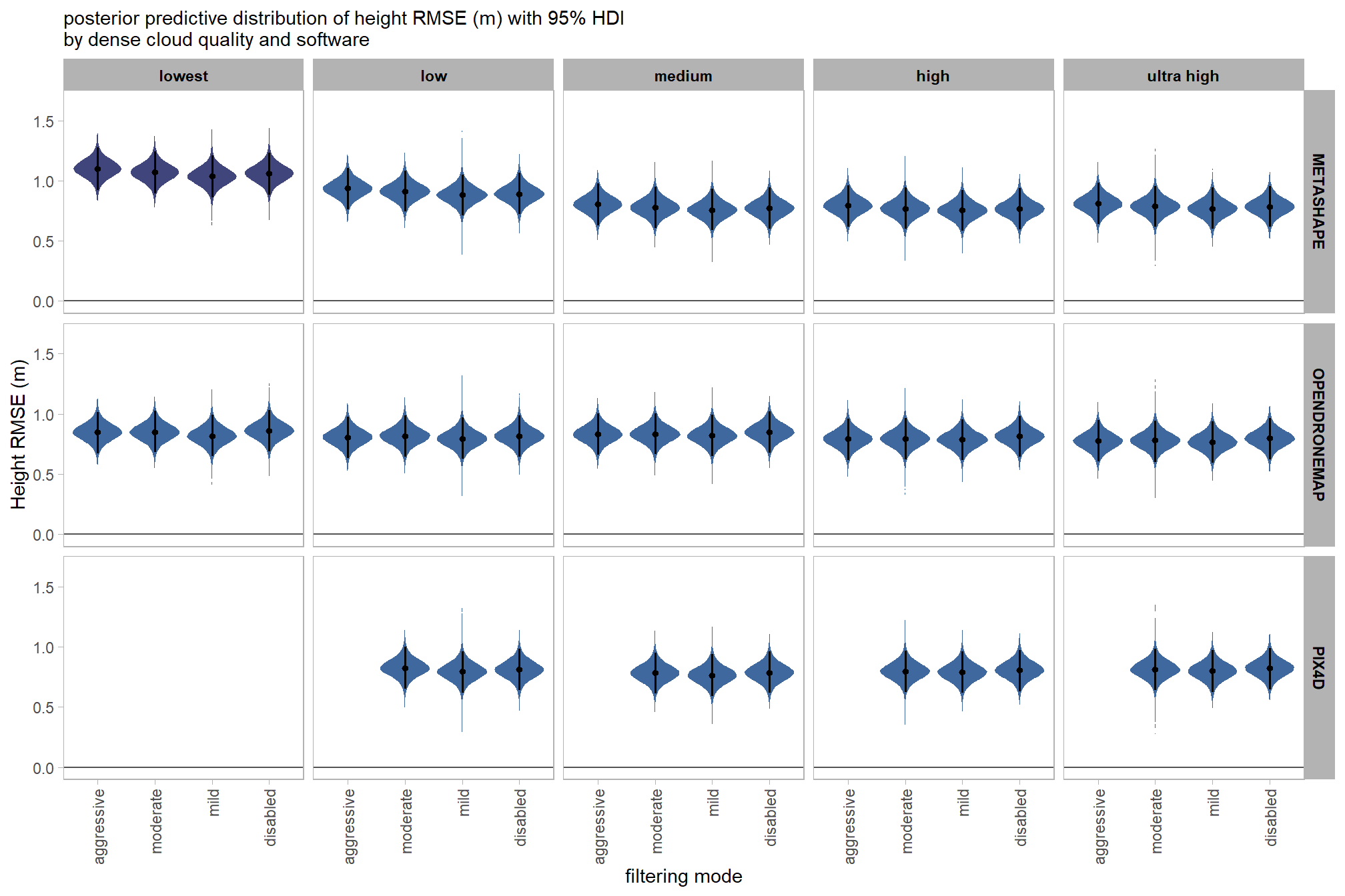
and a table of these 95% HDI values
table_temp =
  fltr_sftwr_draws_temp %>%
  tidybayes::median_hdi(value) %>%
  dplyr::inner_join(
    ptcld_validation_data %>% dplyr::distinct(software, depth_maps_generation_quality, depth_maps_generation_filtering_mode)
    , by = dplyr::join_by(software, depth_maps_generation_quality, depth_maps_generation_filtering_mode)
  ) %>%
  dplyr::mutate(depth_maps_generation_quality = depth_maps_generation_quality %>% forcats::fct_rev()) %>%
  dplyr::select(c(
    software, depth_maps_generation_quality, depth_maps_generation_filtering_mode
    , value, .lower, .upper
  )) %>%
  dplyr::ungroup() %>%
  dplyr::arrange(software, depth_maps_generation_quality, depth_maps_generation_filtering_mode)

table_temp %>%
  # dplyr::select(-c(software)) %>%
  kableExtra::kbl(
    digits = 2
    , caption = "Height RMSE (m)<br>95% HDI of the posterior predictive distribution"
    , col.names = c(
      "software", "quality", "filtering mode"
      , "Height RMSE (m)<br>median"
      , "HDI low", "HDI high"
    )
    , escape = F
  ) %>%
  kableExtra::kable_styling() %>%
  # kableExtra::pack_rows(index = table(forcats::fct_inorder(table_temp$software))) %>%
  kableExtra::collapse_rows(columns = 1:2, valign = "top") %>%
kableExtra::scroll_box(height = "8in")| software | quality | filtering mode |
Height RMSE (m) median |
HDI low | HDI high |
|---|---|---|---|---|---|
| METASHAPE | lowest | aggressive | 1.10 | 0.92 | 1.27 |
| moderate | 1.07 | 0.90 | 1.24 | ||
| mild | 1.04 | 0.86 | 1.21 | ||
| disabled | 1.06 | 0.88 | 1.23 | ||
| low | aggressive | 0.94 | 0.76 | 1.11 | |
| moderate | 0.91 | 0.74 | 1.08 | ||
| mild | 0.88 | 0.71 | 1.05 | ||
| disabled | 0.89 | 0.72 | 1.06 | ||
| medium | aggressive | 0.80 | 0.63 | 0.98 | |
| moderate | 0.78 | 0.61 | 0.95 | ||
| mild | 0.76 | 0.59 | 0.93 | ||
| disabled | 0.77 | 0.60 | 0.94 | ||
| high | aggressive | 0.79 | 0.62 | 0.96 | |
| moderate | 0.77 | 0.60 | 0.94 | ||
| mild | 0.75 | 0.58 | 0.92 | ||
| disabled | 0.77 | 0.59 | 0.94 | ||
| ultra high | aggressive | 0.81 | 0.64 | 0.98 | |
| moderate | 0.79 | 0.61 | 0.96 | ||
| mild | 0.77 | 0.60 | 0.94 | ||
| disabled | 0.78 | 0.61 | 0.96 | ||
| OPENDRONEMAP | lowest | aggressive | 0.85 | 0.67 | 1.02 |
| moderate | 0.85 | 0.68 | 1.03 | ||
| mild | 0.82 | 0.65 | 0.99 | ||
| disabled | 0.86 | 0.69 | 1.03 | ||
| low | aggressive | 0.81 | 0.63 | 0.98 | |
| moderate | 0.82 | 0.64 | 0.99 | ||
| mild | 0.79 | 0.63 | 0.97 | ||
| disabled | 0.82 | 0.65 | 0.99 | ||
| medium | aggressive | 0.83 | 0.66 | 1.00 | |
| moderate | 0.83 | 0.66 | 1.00 | ||
| mild | 0.82 | 0.65 | 0.99 | ||
| disabled | 0.85 | 0.68 | 1.02 | ||
| high | aggressive | 0.79 | 0.62 | 0.96 | |
| moderate | 0.79 | 0.62 | 0.96 | ||
| mild | 0.79 | 0.61 | 0.95 | ||
| disabled | 0.81 | 0.64 | 0.98 | ||
| ultra high | aggressive | 0.77 | 0.60 | 0.95 | |
| moderate | 0.78 | 0.60 | 0.94 | ||
| mild | 0.77 | 0.59 | 0.94 | ||
| disabled | 0.80 | 0.62 | 0.97 | ||
| PIX4D | low | moderate | 0.83 | 0.65 | 1.00 |
| mild | 0.79 | 0.62 | 0.97 | ||
| disabled | 0.81 | 0.64 | 0.99 | ||
| medium | moderate | 0.78 | 0.61 | 0.95 | |
| mild | 0.77 | 0.59 | 0.94 | ||
| disabled | 0.79 | 0.62 | 0.96 | ||
| high | moderate | 0.80 | 0.63 | 0.97 | |
| mild | 0.79 | 0.62 | 0.96 | ||
| disabled | 0.81 | 0.63 | 0.98 | ||
| ultra high | moderate | 0.81 | 0.64 | 0.98 | |
| mild | 0.80 | 0.63 | 0.97 | ||
| disabled | 0.82 | 0.65 | 0.99 |
we can also make pairwise comparisons
# calculate contrast
brms_contrast_temp = fltr_sftwr_draws_temp %>%
  tidybayes::compare_levels(
    value
    , by = depth_maps_generation_filtering_mode
    , comparison = "pairwise"
  ) %>%
  dplyr::rename(contrast = depth_maps_generation_filtering_mode)

# separate contrast
brms_contrast_temp = brms_contrast_temp %>%
  dplyr::ungroup() %>%
  tidyr::separate_wider_delim(
    cols = contrast
    , delim = " - "
    , names = paste0(
      "sorter"
      , 1:(max(stringr::str_count(brms_contrast_temp$contrast, "-"))+1)
    )
    , too_few = "align_start"
    , cols_remove = F
  ) %>%
  dplyr::filter(sorter1!=sorter2) %>%
  dplyr::mutate(
    dplyr::across(
      tidyselect::starts_with("sorter")
      , .fns = function(x){factor(
        x, ordered = T
        , levels = levels(ptcld_validation_data$depth_maps_generation_filtering_mode)
      )}
    )
    , contrast = contrast %>%
      forcats::fct_reorder(
        paste0(as.numeric(sorter1), as.numeric(sorter2)) %>%
          as.numeric()
      ) %>%
      # re order for filtering mode
      forcats::fct_rev()
  ) %>%
  # median_hdi summary for coloring
  dplyr::group_by(contrast, software, depth_maps_generation_quality) %>%
  make_contrast_vars()

# remove out-of-sample obs
brms_contrast_temp = brms_contrast_temp %>%
  dplyr::inner_join(
    ptcld_validation_data %>% dplyr::distinct(software, depth_maps_generation_quality, depth_maps_generation_filtering_mode)
    , by = dplyr::join_by(software, depth_maps_generation_quality, sorter1==depth_maps_generation_filtering_mode)
  ) %>%
  dplyr::inner_join(
    ptcld_validation_data %>% dplyr::distinct(software, depth_maps_generation_quality, depth_maps_generation_filtering_mode)
    , by = dplyr::join_by(software, depth_maps_generation_quality, sorter2==depth_maps_generation_filtering_mode)
  ) %>%
  dplyr::mutate(depth_maps_generation_quality = depth_maps_generation_quality %>% forcats::fct_rev())
plot it
brms_contrast_temp %>%
  plt_contrast(
    facet = c("depth_maps_generation_quality", "software")
    , y_axis_title = "filtering mode"
    , label_size = 0
    , x_expand = c(-0.1,-0.1)
  ) +
  facet_grid(
    rows = vars(software)
    , cols = vars(depth_maps_generation_quality)
  ) +
  labs(
    subtitle = "posterior predictive distribution of group constrasts with 95% & 50% HDI\nby dense cloud quality and software"
    , x = "constrast Height RMSE (m)"
  )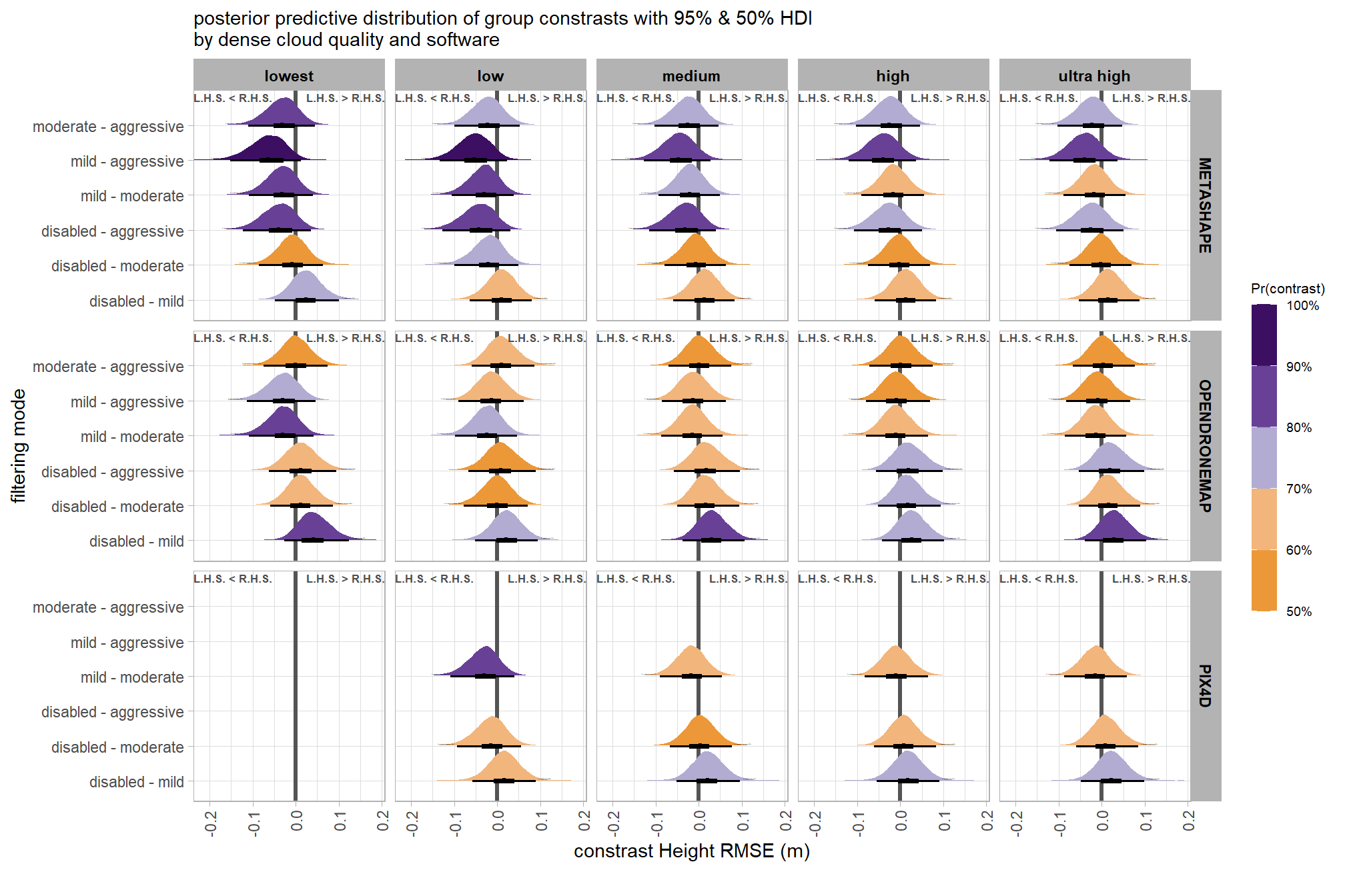
ggplot2::ggsave(
  "../data/qlty_fltr_sftwr_comp_ht_rmse.png"
  , plot = ggplot2::last_plot() + labs(subtitle = "")
  , height = 7, width = 10.5
)
Export some final images for publication
p1_temp = qlty_fltr_sftwr_ht_me + labs(subtitle = "A: Height Mean Error (m)") + theme(plot.subtitle = element_text(face="bold"))
p2_temp = qlty_fltr_sftwr_ht_rmse + labs(subtitle = "B: Height RMSE (m)") + theme(plot.subtitle = element_text(face="bold"))
# export
p1_temp / p2_temp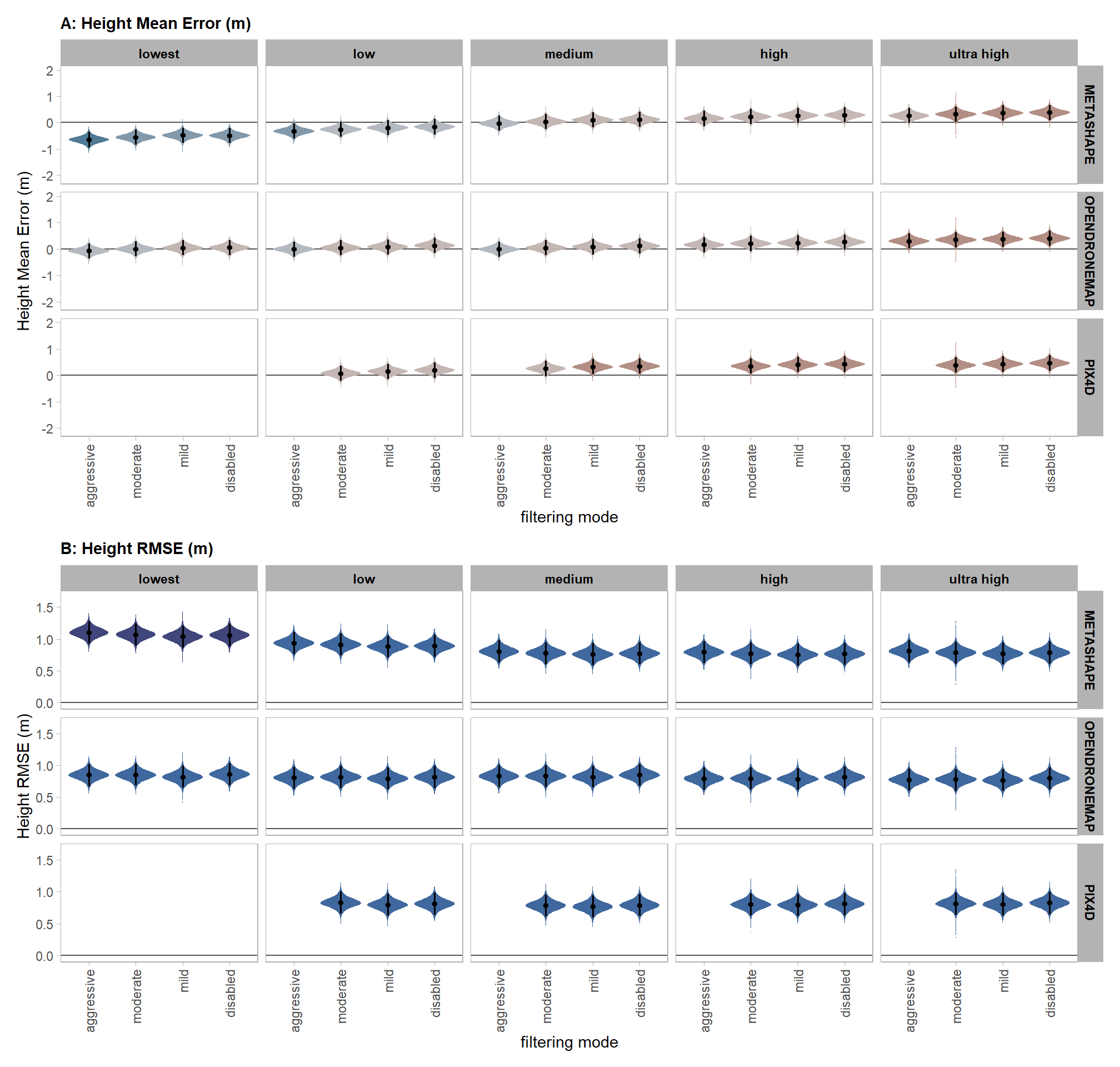
7.4 Tree DBH
7.4.1 Summary Statistics
7.4.1.1 DBH Mean Error (bias)
  # summarize data
  dta_temp = ptcld_validation_data %>%
    dplyr::group_by(software, depth_maps_generation_quality, depth_maps_generation_filtering_mode) %>%
    # collapse across study site
    dplyr::summarise(
      dbh_cm_me = mean(dbh_cm_me, na.rm = T)
      , n = dplyr::n()
    )
  # set limits for color scale
  lmt_dbh_cm_me = ceiling(10*max(abs(range(dta_temp$dbh_cm_me, na.rm = T))))/10
  # scales::show_col(scales::pal_dichromat("BluetoOrange.10")(10))
  # scales::show_col(scales::pal_div_gradient()(seq(0, 1, length.out = 7)))
  # plot it
  dta_temp %>%
    ggplot(mapping = aes(
      y = depth_maps_generation_quality
      , x = depth_maps_generation_filtering_mode
      , fill = dbh_cm_me
      , label = paste0(scales::comma(dbh_cm_me,accuracy = 0.01), "\n(n=", n,")")
    )) +
    geom_tile(color = "white") +
    geom_text(color = "white", size = 3) +
    facet_grid(cols = vars(software)) +
    scale_x_discrete(expand = c(0, 0)) +
    scale_y_discrete(expand = c(0, 0)) +
    scale_fill_stepsn(
      n.breaks = 7
      , colors = scales::pal_div_gradient()(seq(0, 1, length.out = 7))
      , limits = c(-lmt_dbh_cm_me,lmt_dbh_cm_me)
      , labels = scales::comma_format(accuracy = 0.1)
      , show.limits = T
    ) +
    labs(
      x = "filtering mode"
      , y = "quality"
      , fill = "DBH Mean Error (cm)"
      , title = "mean DBH mean error (cm) and # of study sites"
      , subtitle = paste(
        "negative values = UAS tree DBH < field tree DBH"
        , " || "
        , "positive values = UAS tree DBH > field tree DBH"
      )
    ) +
    theme_light() +
    theme(
      legend.position = "none"
      , axis.text.x = element_text(angle = 90, vjust = 0.5, hjust = 1)
      , panel.background = element_blank()
      , panel.grid = element_blank()
      # , plot.title = element_text(hjust = 0.5)
      # , plot.subtitle = element_text(hjust = 0.5)
      , strip.text = element_text(color = "black", face = "bold")
    )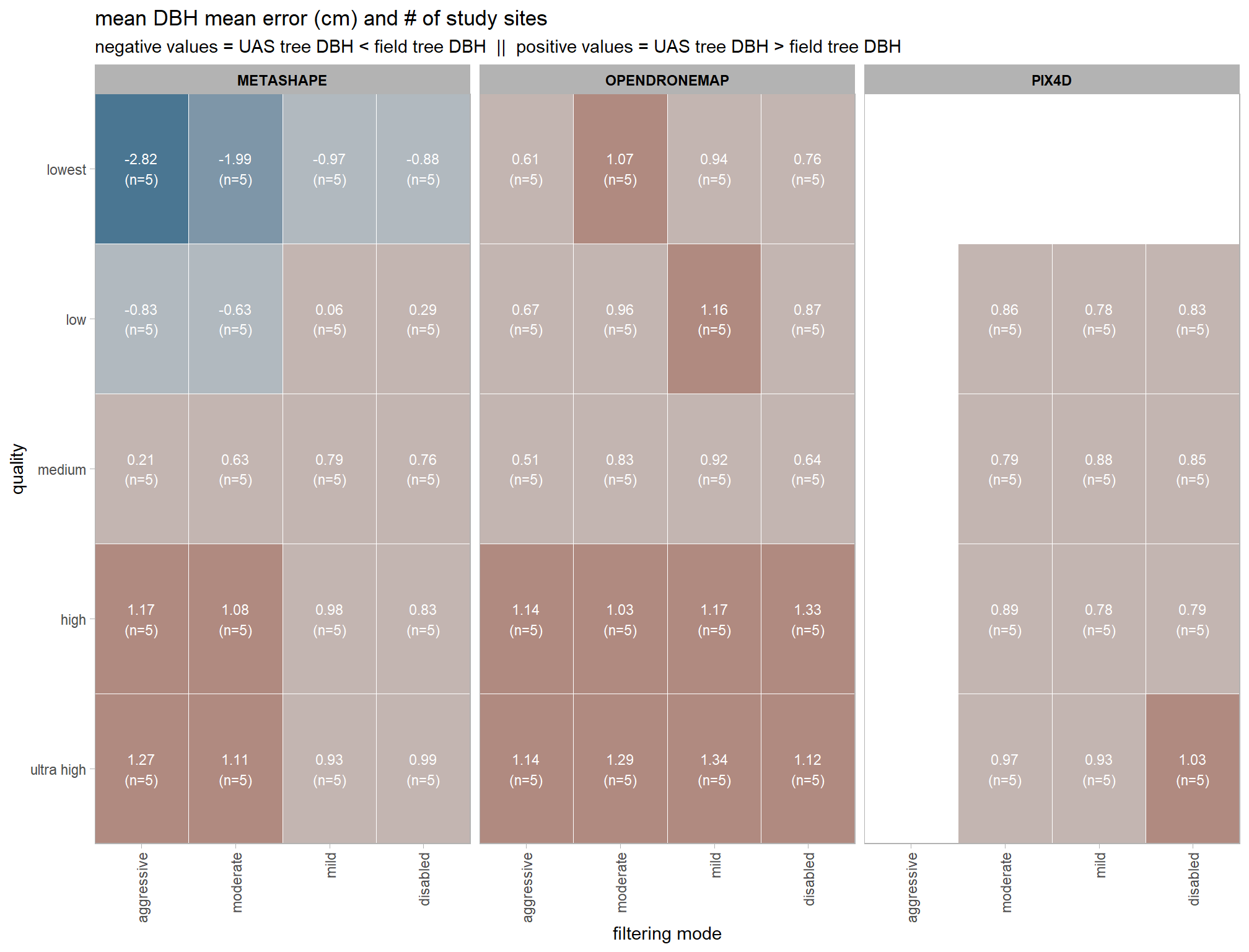
let’s check the distribution (of our dependent or \(y\) variable)
# distribution
ptcld_validation_data %>%
  ggplot(mapping = aes(x = dbh_cm_me)) +
  geom_hline(yintercept = 0, color = "gray77") +
  geom_vline(xintercept = 0, color = "gray77") +
  # geom_vline(xintercept = c(0,1)) +
  geom_density(fill = "lightblue", alpha = 0.7, color = NA) +
  labs(y="",x="DBH Mean Error (cm)") +
  scale_y_continuous(breaks = c(0)) +
  scale_x_continuous(breaks = scales::extended_breaks(10)) +
  theme_light() +
  theme(panel.grid = element_blank())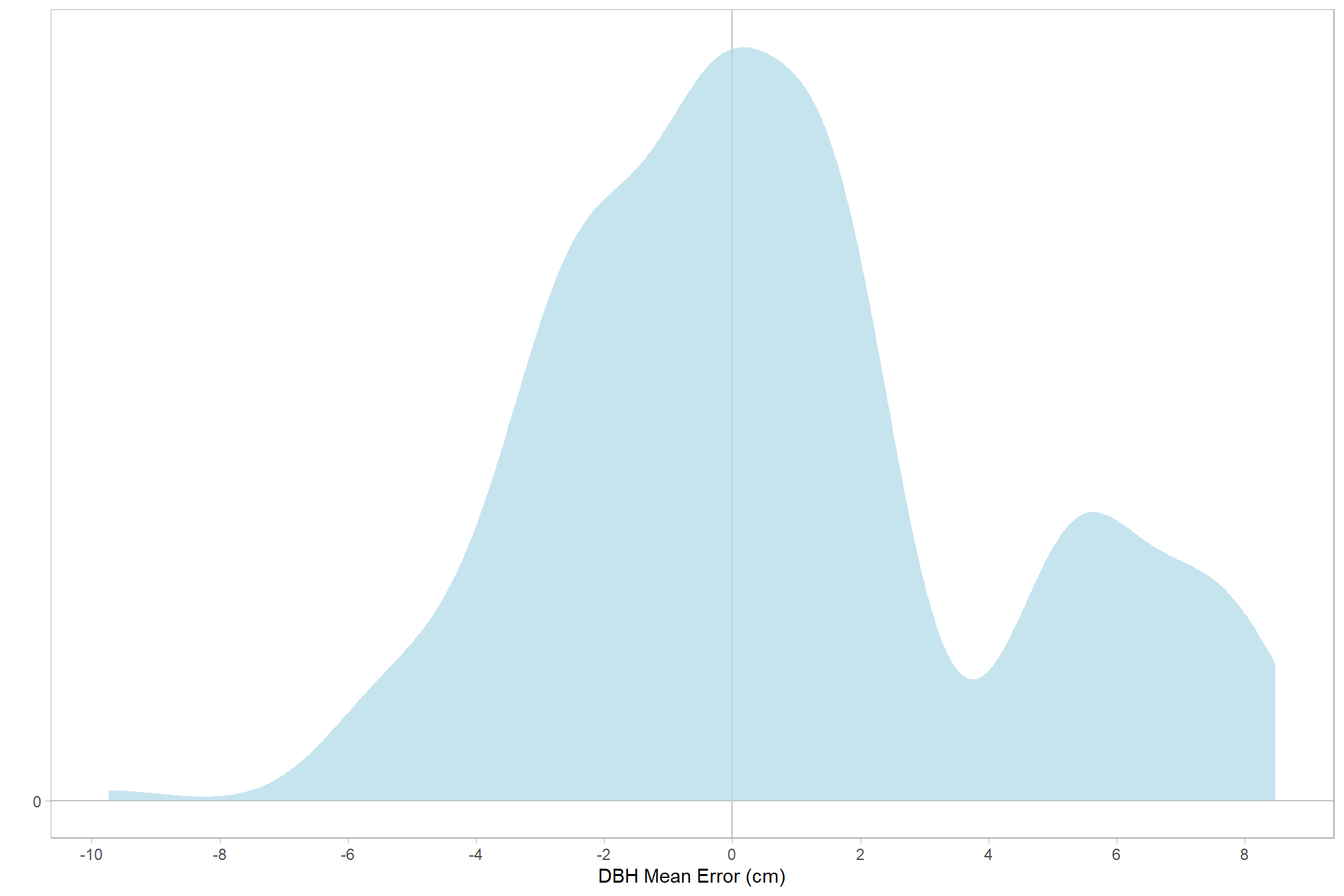
and the summary statistics
ptcld_validation_data %>%
  dplyr::ungroup() %>%
  dplyr::select(dbh_cm_me) %>%
  dplyr::summarise(
    dplyr::across(
      dplyr::everything()
      , .fns = list(
        mean = ~ mean(.x,na.rm=T), median = ~ median(.x,na.rm=T), sd = ~ sd(.x,na.rm=T)
        , min = ~ min(.x,na.rm=T), max = ~ max(.x,na.rm=T)
        , q25 = ~ quantile(.x, 0.25, na.rm = T)
        , q75 = ~ quantile(.x, 0.75, na.rm = T)
      )
      , .names = "{.fn}"
    )
  ) %>%
  tidyr::pivot_longer(everything()) %>%
  kableExtra::kbl(caption = "summary: `dbh_cm_me`", digits = 3, col.names = NULL) %>%
kableExtra::kable_styling()| mean | 0.655 |
| median | 0.149 |
| sd | 3.506 |
| min | -9.733 |
| max | 8.480 |
| q25 | -1.964 |
| q75 | 2.003 |
7.4.1.2 DBH RMSE (precision)
  # summarize data
  dta_temp = ptcld_validation_data %>%
    dplyr::group_by(software, depth_maps_generation_quality, depth_maps_generation_filtering_mode) %>%
    # collapse across study site
    dplyr::summarise(
      dbh_cm_rmse = mean(dbh_cm_rmse, na.rm = T)
      , n = dplyr::n()
    )
  # set limits for color scale
  lmt_dbh_cm_rmse = ceiling(1.02*10*max(abs(range(dta_temp$dbh_cm_rmse, na.rm = T))))/10
  # scales::show_col(viridis::mako(n = 10, begin = 0.2, end = 0.9, direction = -1))
  # scales::show_col(scales::pal_div_gradient()(seq(0, 1, length.out = 7)))
  # plot it
  dta_temp %>%
    ggplot(mapping = aes(
      y = depth_maps_generation_quality
      , x = depth_maps_generation_filtering_mode
      , fill = dbh_cm_rmse
      , label = paste0(scales::comma(dbh_cm_rmse,accuracy = 0.1), "\n(n=", n,")")
    )) +
    geom_tile(color = "white") +
    geom_text(color = "white", size = 3) +
    facet_grid(cols = vars(software)) +
    scale_x_discrete(expand = c(0, 0)) +
    scale_y_discrete(expand = c(0, 0)) +
    scale_fill_stepsn(
      n.breaks = 5
      , colors = viridis::mako(n = 5, begin = 0.2, end = 0.9, direction = -1)
      , limits = c(0,lmt_dbh_cm_rmse)
      , labels = scales::comma_format(accuracy = 0.1)
      , show.limits = T
    ) +
    labs(
      x = "filtering mode"
      , y = "quality"
      , fill = "DBH RMSE (cm)"
      , title = "mean DBH RMSE (cm) and # of study sites"
    ) +
    theme_light() +
    theme(
      legend.position = "none"
      , axis.text.x = element_text(angle = 90, vjust = 0.5, hjust = 1)
      , panel.background = element_blank()
      , panel.grid = element_blank()
      # , plot.title = element_text(hjust = 0.5)
      # , plot.subtitle = element_text(hjust = 0.5)
      , strip.text = element_text(color = "black", face = "bold")
    )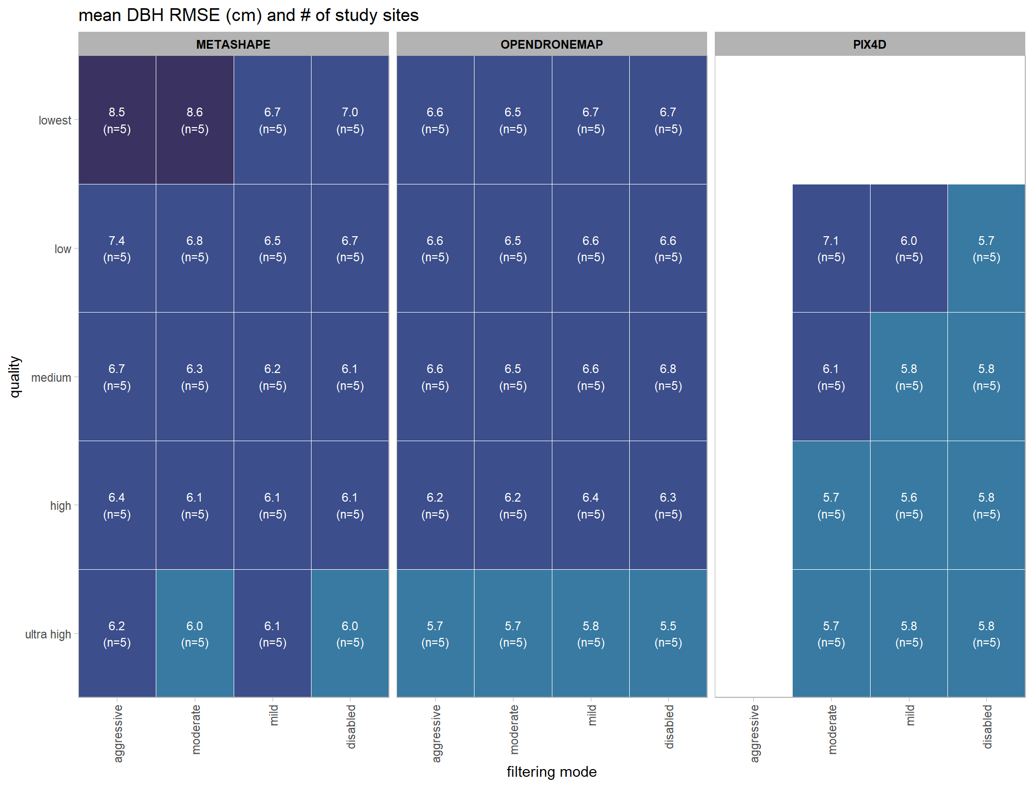
let’s check the distribution (of our dependent or \(y\) variable)
# distribution
ptcld_validation_data %>%
  ggplot(mapping = aes(x = dbh_cm_rmse)) +
  geom_hline(yintercept = 0, color = "gray77") +
  geom_vline(xintercept = 0, color = "gray77") +
  # geom_vline(xintercept = c(0,1)) +
  geom_density(fill = "lightblue", alpha = 0.7, color = NA) +
  labs(y="",x="DBH RMSE (cm)") +
  scale_y_continuous(breaks = c(0)) +
  scale_x_continuous(breaks = scales::extended_breaks(10)) +
  theme_light() +
  theme(panel.grid = element_blank())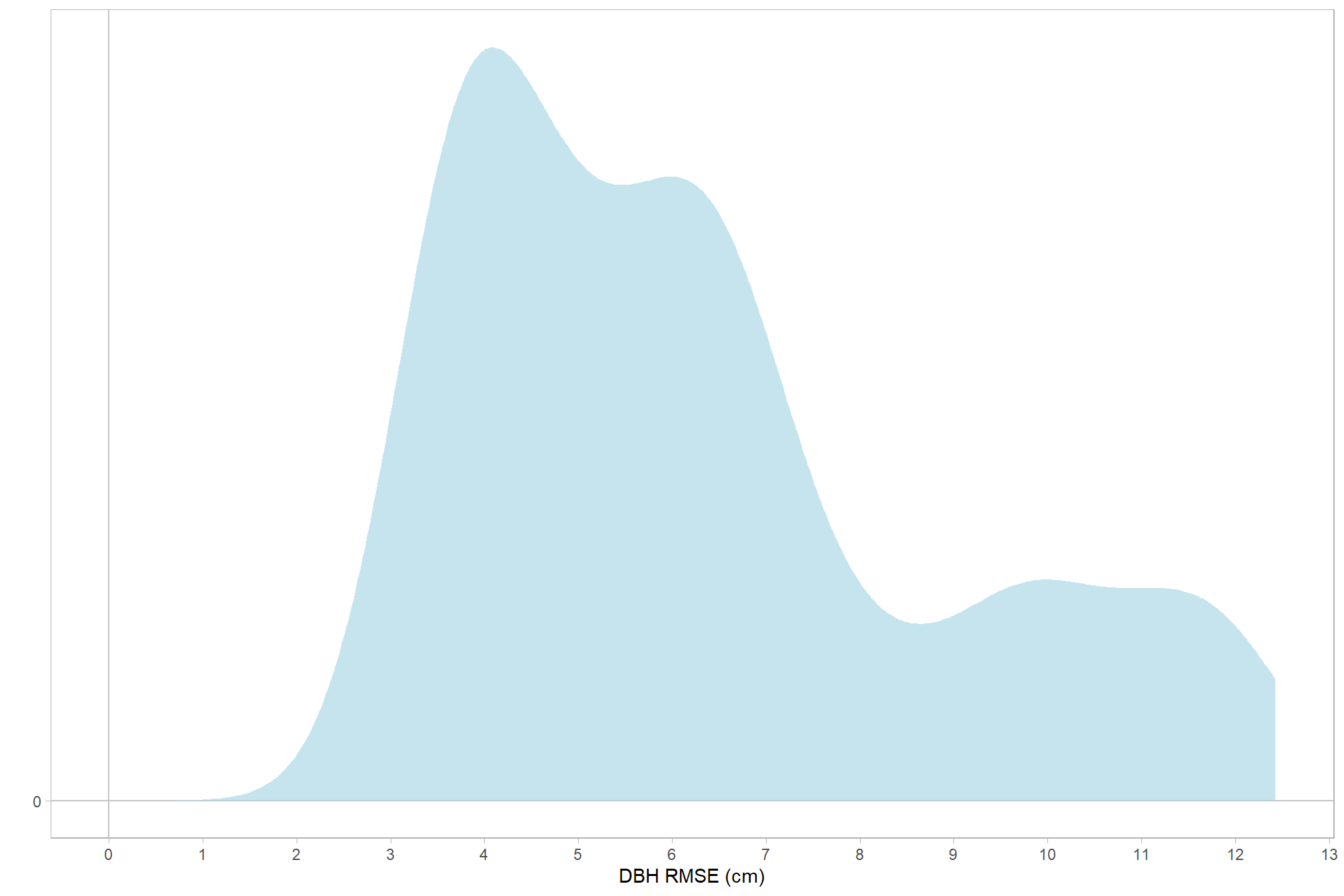
and the summary statistics
ptcld_validation_data %>%
  dplyr::ungroup() %>%
  dplyr::select(dbh_cm_rmse) %>%
  dplyr::summarise(
    dplyr::across(
      dplyr::everything()
      , .fns = list(
        mean = ~ mean(.x,na.rm=T), median = ~ median(.x,na.rm=T), sd = ~ sd(.x,na.rm=T)
        , min = ~ min(.x,na.rm=T), max = ~ max(.x,na.rm=T)
        , q25 = ~ quantile(.x, 0.25, na.rm = T)
        , q75 = ~ quantile(.x, 0.75, na.rm = T)
      )
      , .names = "{.fn}"
    )
  ) %>%
  tidyr::pivot_longer(everything()) %>%
  kableExtra::kbl(caption = "summary: `dbh_cm_rmse`", digits = 3, col.names = NULL) %>%
kableExtra::kable_styling()| mean | 6.337 |
| median | 5.869 |
| sd | 2.566 |
| min | 3.272 |
| max | 12.430 |
| q25 | 4.080 |
| q75 | 7.414 |
7.4.2 Model: DBH Mean Error (bias)
Define priors
# from Kurz:
gamma_a_b_from_omega_sigma = function(mode, sd) {
  if (mode <= 0) stop("mode must be > 0")
  if (sd   <= 0) stop("sd must be > 0")
  rate = (mode + sqrt(mode^2 + 4 * sd^2)) / (2 * sd^2)
  shape = 1 + mode * rate
  return(list(shape = shape, rate = rate))
}

mean_y_temp = mean(ptcld_validation_data$dbh_cm_me, na.rm = T)
sd_y_temp   = sd(ptcld_validation_data$dbh_cm_me, na.rm = T)

omega_temp = sd_y_temp / 2
sigma_temp = 2 * sd_y_temp

s_r_temp = gamma_a_b_from_omega_sigma(mode = omega_temp, sd = sigma_temp)

stanvars_temp =
  brms::stanvar(mean_y_temp,    name = "mean_y") +
  brms::stanvar(sd_y_temp,      name = "sd_y") +
  brms::stanvar(s_r_temp$shape, name = "alpha") +
  brms::stanvar(s_r_temp$rate,  name = "beta")
7.4.2.1 Prior distributions
#### setting priors
# required libraries: tidyverse, tidybayes, brms, palettetown, latex2exp
priors_temp <- c(
    brms::prior(normal(mean_y_temp, sd_y_temp * 5), class = "Intercept")
    , brms::prior(gamma(s_r_temp$shape, s_r_temp$rate), class = "sd")
    , brms::prior(cauchy(0, sd_y_temp), class = "sigma")
  )
# plot
plt_prior3 =
priors_temp %>%
  tidybayes::parse_dist() %>%
  tidybayes::marginalize_lkjcorr(K = 2) %>%
  tidyr::separate(
    .args
    , sep = ","
    , into = c("a","b")
    , remove = F
  ) %>%
  dplyr::mutate(
    distrib = paste0(
      class, " ~ "
      , .dist
      , "("
      , a %>% readr::parse_number() %>% round(2)
      , ","
      , b %>% readr::parse_number() %>% round(2)
      , ")"
    )
  ) %>%
  ggplot(., aes(dist = .dist, args = .args)) +
  facet_grid(cols=vars(distrib), scales = "free") +
  ggdist::stat_halfeye(
    aes(fill = prior),
    n = 10e2,
    show.legend = F
    , fill = "slategray"
  ) +
  coord_flip() +
  theme_light() +
  theme(
    strip.text = element_text(face = "bold", color = "black"),
    axis.text.y = element_blank(),
    axis.ticks = element_blank()
    , axis.text = element_text(size = 6)
  )+
  labs(
    x = ""
    , title = "Priors: DBH Mean Error (bias)"
    , y = ""
  )
plt_prior3
7.4.2.2 Fit the model
Now fit the model.
brms_dbh_me_mod = brms::brm(
  formula = dbh_cm_me ~
    # baseline
    1 +
    # main effects
    (1 | depth_maps_generation_quality) +
    (1 | depth_maps_generation_filtering_mode) +
    (1 | software) +
    (1 | study_site) + # only fitting main effects of site and not interactions
    # two-way interactions
    (1 | depth_maps_generation_quality:depth_maps_generation_filtering_mode) +
    (1 | depth_maps_generation_quality:software) +
    (1 | depth_maps_generation_filtering_mode:software) +
    # three-way interactions
    (1 | depth_maps_generation_quality:depth_maps_generation_filtering_mode:software)
  , data = ptcld_validation_data
  , family = brms::brmsfamily(family = "gaussian")
  , iter = 20000, warmup = 10000, chains = 4
  , control = list(adapt_delta = 0.999, max_treedepth = 13)
  , cores = round(parallel::detectCores()/2)
  , prior = c(
    brms::prior(normal(mean_y, sd_y * 5), class = "Intercept")
    , brms::prior(gamma(alpha, beta), class = "sd")
    , brms::prior(cauchy(0, sd_y), class = "sigma")
  )
  , stanvars = stanvars_temp
  , file = paste0(rootdir, "/fits/brms_dbh_me_mod")
)
7.4.2.3 Quality:Filtering - interaction
draws_temp =
  ptcld_validation_data %>%
    dplyr::distinct(depth_maps_generation_quality, depth_maps_generation_filtering_mode) %>%
    tidybayes::add_epred_draws(
      brms_dbh_me_mod, allow_new_levels = T
      # this part is crucial
      , re_formula = ~ (1 | depth_maps_generation_quality) +
        (1 | depth_maps_generation_filtering_mode) +
        (1 | depth_maps_generation_quality:depth_maps_generation_filtering_mode)
    ) %>%
    dplyr::rename(value = .epred) %>%
    dplyr::mutate(med = tidybayes::median_hdci(value)$y)
# plot
  draws_temp %>%
    dplyr::mutate(depth_maps_generation_quality = depth_maps_generation_quality %>% forcats::fct_rev()) %>%
  # plot
  ggplot(
    mapping = aes(
      y = value, x = depth_maps_generation_filtering_mode
      , fill = med
    )
  ) +
    geom_hline(yintercept = 0, color = "gray33") +
    # tidybayes::stat_dotsinterval(
    #   point_interval = median_hdi, .width = .95
    #   , justification = -0.04
    #   , slab_alpha = 0.98
    #   , shape = 21, point_size = 3
    #   , quantiles = 100
    # ) +
    tidybayes::stat_eye(
      point_interval = median_hdi, .width = .95
      , slab_alpha = 0.98
      , interval_color = "black", linewidth = 1
      , point_color = "black", point_fill = "black", point_size = 1
    ) +
    scale_fill_stepsn(
      n.breaks = 7
      , colors = scales::pal_div_gradient()(seq(0, 1, length.out = 7))
      , limits = c(-lmt_dbh_cm_me*0.7,lmt_dbh_cm_me*0.7)
      , labels = scales::comma_format(accuracy = 0.1)
      , show.limits = T
    ) +
    scale_y_continuous(breaks = scales::extended_breaks(n=8)) +
    facet_grid(cols = vars(depth_maps_generation_quality)) +
    labs(
      x = "filtering mode", y = "DBH Mean Error (cm)"
      , subtitle = "posterior predictive distribution of DBH mean error (cm) with 95% HDI\nby dense cloud quality"
    ) +
    theme_light() +
    theme(
      legend.position = "none"
      , legend.direction  = "horizontal"
      , axis.text.x = element_text(angle = 90, vjust = 0.5, hjust = 1)
      , strip.text = element_text(color = "black", face = "bold")
) 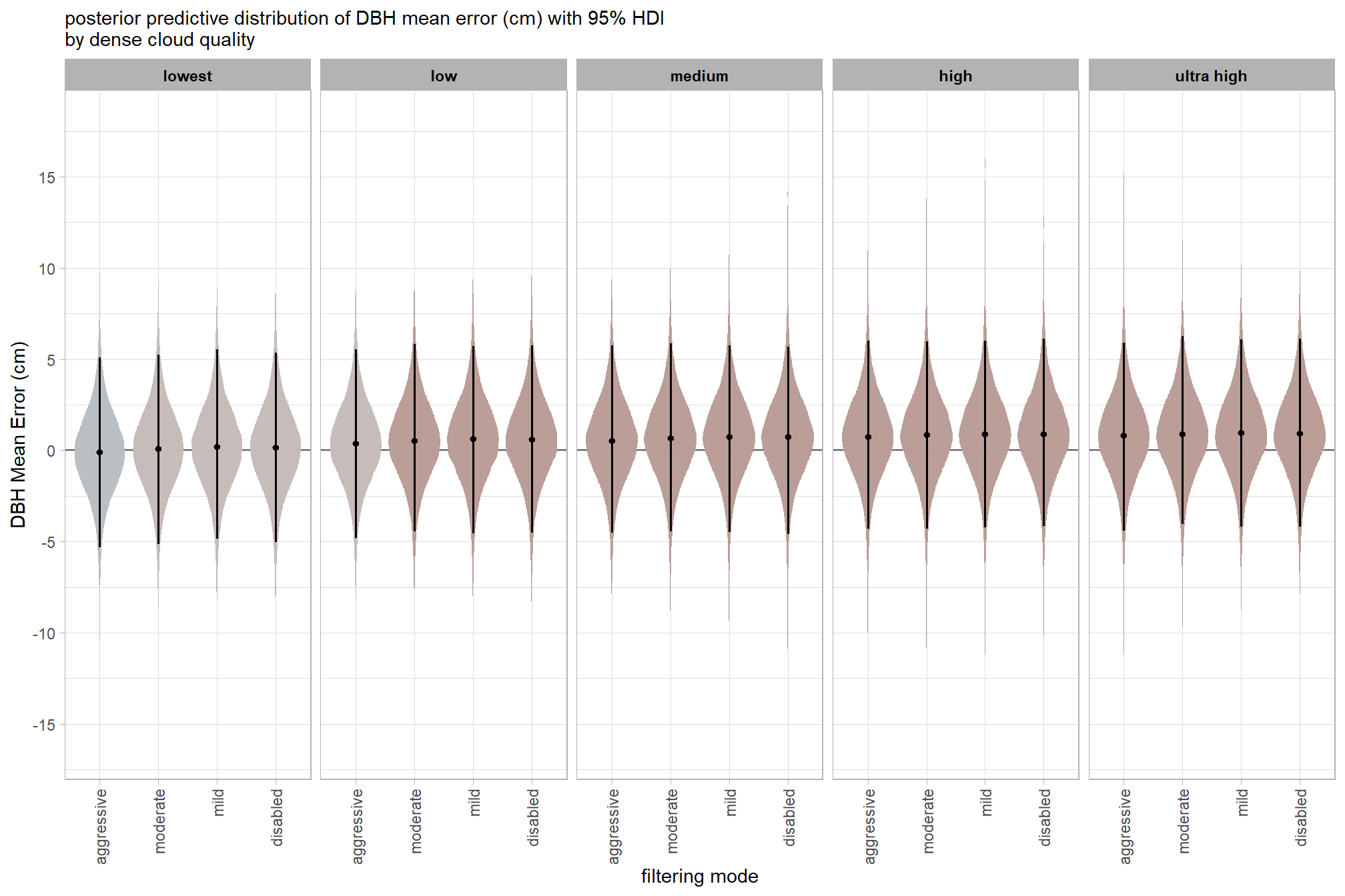
and a table of these 95% HDI values
table_temp =
  draws_temp %>%
    tidybayes::median_hdi(value) %>%
    dplyr::select(-c(.point,.interval, .width,.row)) %>%
    dplyr::arrange(depth_maps_generation_quality,depth_maps_generation_filtering_mode)

table_temp %>%
  dplyr::select(-c(depth_maps_generation_quality)) %>%
  kableExtra::kbl(
    digits = 2
    , caption = "DBH Mean Error (cm)<br>95% HDI of the posterior predictive distribution"
    , col.names = c(
      "filtering mode"
      , "DBH Mean Error (cm)<br>median"
      , "HDI low", "HDI high"
    )
    , escape = F
  ) %>%
  kableExtra::kable_styling() %>%
  kableExtra::pack_rows(index = table(forcats::fct_inorder(table_temp$depth_maps_generation_quality))) %>%
kableExtra::scroll_box(height = "8in")| filtering mode |
DBH Mean Error (cm) median |
HDI low | HDI high |
|---|---|---|---|
| ultra high | |||
| aggressive | 0.82 | -4.39 | 5.91 |
| moderate | 0.91 | -4.03 | 6.25 |
| mild | 0.96 | -4.20 | 6.07 |
| disabled | 0.94 | -4.19 | 6.11 |
| high | |||
| aggressive | 0.75 | -4.28 | 6.02 |
| moderate | 0.85 | -4.29 | 5.98 |
| mild | 0.90 | -4.23 | 6.02 |
| disabled | 0.89 | -4.17 | 6.12 |
| medium | |||
| aggressive | 0.54 | -4.51 | 5.76 |
| moderate | 0.69 | -4.43 | 5.85 |
| mild | 0.76 | -4.48 | 5.77 |
| disabled | 0.73 | -4.60 | 5.67 |
| low | |||
| aggressive | 0.38 | -4.80 | 5.54 |
| moderate | 0.52 | -4.45 | 5.83 |
| mild | 0.62 | -4.56 | 5.73 |
| disabled | 0.61 | -4.53 | 5.76 |
| lowest | |||
| aggressive | -0.11 | -5.34 | 5.10 |
| moderate | 0.07 | -5.14 | 5.24 |
| mild | 0.19 | -4.85 | 5.53 |
| disabled | 0.17 | -5.03 | 5.35 |
7.4.2.4 Software:Quality - interaction
draws_temp =
  ptcld_validation_data %>%
    dplyr::distinct(depth_maps_generation_quality, software) %>%
    tidybayes::add_epred_draws(
      brms_dbh_me_mod, allow_new_levels = T
      # this part is crucial
      , re_formula = ~ (1 | depth_maps_generation_quality) +
        (1 | software) +
        (1 | depth_maps_generation_quality:software)
    ) %>%
    dplyr::rename(value = .epred) %>%
    dplyr::mutate(med = tidybayes::median_hdci(value)$y)
# plot
  draws_temp %>%
    dplyr::mutate(depth_maps_generation_quality = depth_maps_generation_quality %>% forcats::fct_rev()) %>%
  # plot
  ggplot(
    mapping = aes(
      y = value, x = software
      , fill = med
    )
  ) +
    geom_hline(yintercept = 0, color = "gray33") +
    tidybayes::stat_eye(
      point_interval = median_hdi, .width = .95
      , slab_alpha = 0.98
      , interval_color = "black", linewidth = 1
      , point_color = "black", point_fill = "black", point_size = 1
    ) +
    scale_fill_stepsn(
      n.breaks = 7
      , colors = scales::pal_div_gradient()(seq(0, 1, length.out = 7))
      , limits = c(-lmt_dbh_cm_me*0.7,lmt_dbh_cm_me*0.7)
      , labels = scales::comma_format(accuracy = 0.1)
      , show.limits = T
    ) +
    scale_y_continuous(breaks = scales::extended_breaks(n=8)) +
    facet_grid(cols = vars(depth_maps_generation_quality)) +
    labs(
      x = "software", y = "DBH Mean Error (cm)"
      , subtitle = "posterior predictive distribution of DBH mean error (cm) with 95% HDI\nby dense cloud quality"
    ) +
    theme_light() +
    theme(
      legend.position = "none"
      , legend.direction  = "horizontal"
      , axis.text.x = element_text(angle = 90, vjust = 0.5, hjust = 1)
      , strip.text = element_text(color = "black", face = "bold")
) 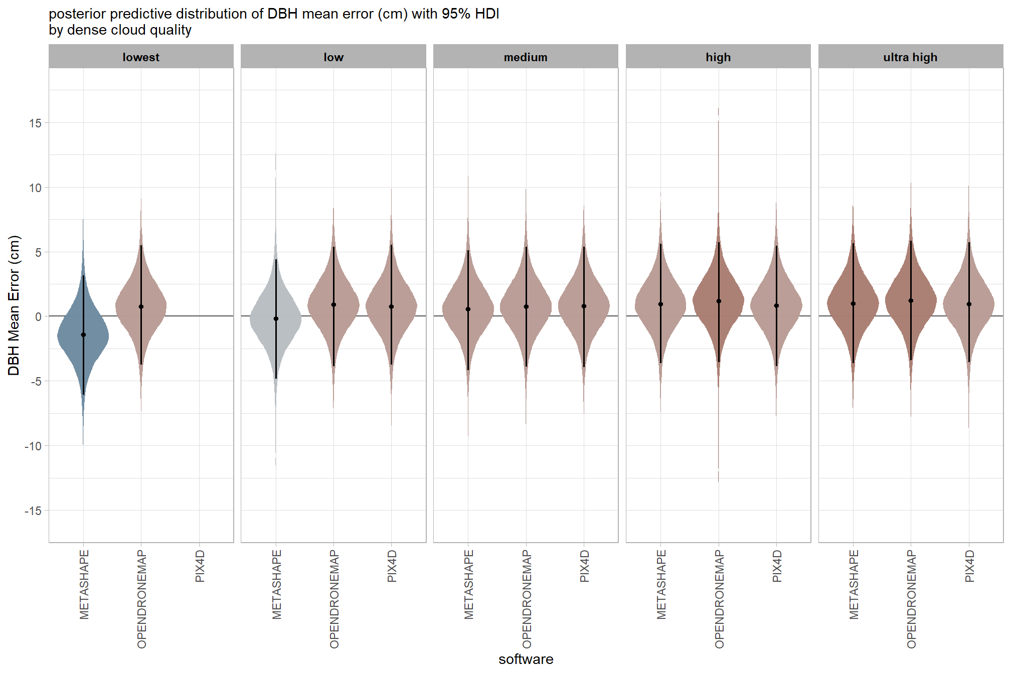
and a table of these 95% HDI values
table_temp =
  draws_temp %>%
  tidybayes::median_hdi(value) %>%
  # remove out-of-sample obs
    dplyr::inner_join(
      ptcld_validation_data %>% dplyr::distinct(depth_maps_generation_quality, software)
      , by = dplyr::join_by(depth_maps_generation_quality, software)
    ) %>%
  dplyr::select(-c(.point,.interval, .width,.row)) %>%
  dplyr::arrange(software,depth_maps_generation_quality)

table_temp %>%
  dplyr::select(-c(software)) %>%
  kableExtra::kbl(
    digits = 2
    , caption = "DBH Mean Error (cm)<br>95% HDI of the posterior predictive distribution"
    , col.names = c(
      "quality"
      , "DBH Mean Error (cm)<br>median"
      , "HDI low", "HDI high"
    )
    , escape = F
  ) %>%
  kableExtra::kable_styling() %>%
  kableExtra::pack_rows(index = table(forcats::fct_inorder(table_temp$software))) %>%
kableExtra::scroll_box(height = "8in")| quality |
DBH Mean Error (cm) median |
HDI low | HDI high |
|---|---|---|---|
| METASHAPE | |||
| ultra high | 1.00 | -3.64 | 5.65 |
| high | 0.95 | -3.62 | 5.61 |
| medium | 0.57 | -4.19 | 5.08 |
| low | -0.18 | -4.83 | 4.42 |
| lowest | -1.42 | -6.09 | 3.16 |
| OPENDRONEMAP | |||
| ultra high | 1.23 | -3.40 | 5.85 |
| high | 1.17 | -3.54 | 5.73 |
| medium | 0.76 | -3.90 | 5.38 |
| low | 0.90 | -3.86 | 5.38 |
| lowest | 0.77 | -3.76 | 5.48 |
| PIX4D | |||
| ultra high | 0.95 | -3.55 | 5.71 |
| high | 0.82 | -3.86 | 5.45 |
| medium | 0.79 | -3.96 | 5.35 |
| low | 0.75 | -3.74 | 5.54 |
7.4.2.5 Software:Filtering - interaction
draws_temp =
  ptcld_validation_data %>%
    dplyr::distinct(depth_maps_generation_filtering_mode, software) %>%
    tidybayes::add_epred_draws(
      brms_dbh_me_mod, allow_new_levels = T
      # this part is crucial
      , re_formula = ~ (1 | depth_maps_generation_filtering_mode) +
        (1 | software) +
        (1 | depth_maps_generation_filtering_mode:software)
    ) %>%
    dplyr::rename(value = .epred) %>%
    dplyr::mutate(med = tidybayes::median_hdci(value)$y)
# plot
  draws_temp %>%
  # plot
  ggplot(
    mapping = aes(
      y = value, x = software
      , fill = med
    )
  ) +
    geom_hline(yintercept = 0, color = "gray33") +
    tidybayes::stat_eye(
      point_interval = median_hdi, .width = .95
      , slab_alpha = 0.98
      , interval_color = "black", linewidth = 1
      , point_color = "black", point_fill = "black", point_size = 1
    ) +
    scale_fill_stepsn(
      n.breaks = 7
      , colors = scales::pal_div_gradient()(seq(0, 1, length.out = 7))
      , limits = c(-lmt_dbh_cm_me*0.7,lmt_dbh_cm_me*0.7)
      , labels = scales::comma_format(accuracy = 0.1)
      , show.limits = T
    ) +
    scale_y_continuous(breaks = scales::extended_breaks(n=8)) +
    facet_grid(cols = vars(depth_maps_generation_filtering_mode)) +
    labs(
      x = "software", y = "DBH Mean Error (cm)"
      , subtitle = "posterior predictive distribution of DBH mean error (cm) with 95% HDI\nby filtering mode"
    ) +
    theme_light() +
    theme(
      legend.position = "none"
      , legend.direction  = "horizontal"
      , axis.text.x = element_text(angle = 90, vjust = 0.5, hjust = 1)
      , strip.text = element_text(color = "black", face = "bold")
) 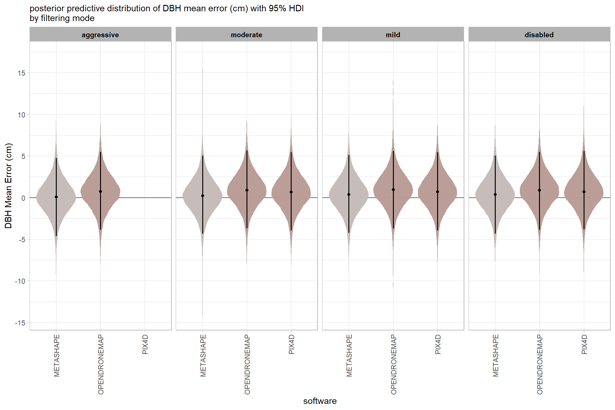
and a table of these 95% HDI values
table_temp =
  draws_temp %>%
    tidybayes::median_hdi(value) %>%
    dplyr::select(-c(.point,.interval, .width,.row)) %>%
    dplyr::arrange(software,depth_maps_generation_filtering_mode)

table_temp %>%
  dplyr::select(-c(software)) %>%
  kableExtra::kbl(
    digits = 2
    , caption = "DBH Mean Error (cm)<br>95% HDI of the posterior predictive distribution"
    , col.names = c(
      "filtering mode"
      , "DBH Mean Error (cm)<br>median"
      , "HDI low", "HDI high"
    )
    , escape = F
  ) %>%
  kableExtra::kable_styling() %>%
  kableExtra::pack_rows(index = table(forcats::fct_inorder(table_temp$software))) %>%
kableExtra::scroll_box(height = "8in")| filtering mode |
DBH Mean Error (cm) median |
HDI low | HDI high |
|---|---|---|---|
| METASHAPE | |||
| aggressive | 0.09 | -4.63 | 4.74 |
| moderate | 0.24 | -4.35 | 5.03 |
| mild | 0.38 | -4.25 | 5.12 |
| disabled | 0.37 | -4.33 | 5.03 |
| OPENDRONEMAP | |||
| aggressive | 0.76 | -3.87 | 5.47 |
| moderate | 0.90 | -3.68 | 5.66 |
| mild | 0.97 | -3.73 | 5.60 |
| disabled | 0.91 | -3.88 | 5.48 |
| PIX4D | |||
| moderate | 0.68 | -3.95 | 5.43 |
| mild | 0.73 | -3.93 | 5.43 |
| disabled | 0.72 | -3.79 | 5.59 |
7.4.2.6 Software:Quality:Filtering - interaction
# get draws
fltr_sftwr_draws_temp =
  tidyr::crossing(
    depth_maps_generation_quality = unique(ptcld_validation_data$depth_maps_generation_quality)
    , depth_maps_generation_filtering_mode = unique(ptcld_validation_data$depth_maps_generation_filtering_mode)
    , software = unique(ptcld_validation_data$software)
  ) %>%
  tidybayes::add_epred_draws(
    brms_dbh_me_mod, allow_new_levels = T
    # this part is crucial
    , re_formula = ~ (1 | depth_maps_generation_quality) + # main effects
    (1 | depth_maps_generation_quality) +
    (1 | depth_maps_generation_filtering_mode) +
    (1 | software) +
    # two-way interactions
    (1 | depth_maps_generation_quality:depth_maps_generation_filtering_mode) +
    (1 | depth_maps_generation_quality:software) +
    (1 | depth_maps_generation_filtering_mode:software) +
    # three-way interactions
    (1 | depth_maps_generation_quality:depth_maps_generation_filtering_mode:software)
  ) %>%
  dplyr::rename(value = .epred) %>%
  dplyr::mutate(med = tidybayes::median_hdci(value)$y)

# plot
qlty_fltr_sftwr_dbh_me =
  fltr_sftwr_draws_temp %>%
    dplyr::inner_join(
      ptcld_validation_data %>% dplyr::distinct(software, depth_maps_generation_quality, depth_maps_generation_filtering_mode)
      , by = dplyr::join_by(software, depth_maps_generation_quality, depth_maps_generation_filtering_mode)
    ) %>%
    dplyr::mutate(depth_maps_generation_quality = depth_maps_generation_quality %>% forcats::fct_rev()) %>%
    ggplot(
      mapping = aes(
        y = value
        , x = depth_maps_generation_filtering_mode
        , fill = med
      )
    ) +
    geom_hline(yintercept = 0, color = "gray33") +
    tidybayes::stat_eye(
      point_interval = median_hdi, .width = .95
      , slab_alpha = 0.98
      , interval_color = "black", linewidth = 1
      , point_color = "black", point_fill = "black", point_size = 1
    ) +
    scale_fill_stepsn(
      n.breaks = 7
      , colors = scales::pal_div_gradient()(seq(0, 1, length.out = 7))
      , limits = c(-lmt_dbh_cm_me*0.7,lmt_dbh_cm_me*0.7)
      , labels = scales::comma_format(accuracy = 0.1)
      , show.limits = T
    ) +
    facet_grid(
      rows = vars(software)
      , cols = vars(depth_maps_generation_quality)
      # , switch = "y"
    ) +
    labs(
      x = "filtering mode", y = "DBH Mean Error (cm)"
      , subtitle = "posterior predictive distribution of DBH mean error (cm) with 95% HDI\nby dense cloud quality and software"
      # , caption = form_temp
    ) +
    theme_light() +
    theme(
      legend.position = "none"
      , legend.direction  = "horizontal"
      , axis.text.x = element_text(angle = 90, vjust = 0.5, hjust = 1)
      , strip.text = element_text(color = "black", face = "bold")
      , panel.grid = element_blank()
      # , strip.placement = "outside"
    ) +
    guides(
      fill = guide_legend(override.aes = list(shape = NA, size = 6, alpha = 0.9, lwd = NA))
    )
# print it
qlty_fltr_sftwr_dbh_me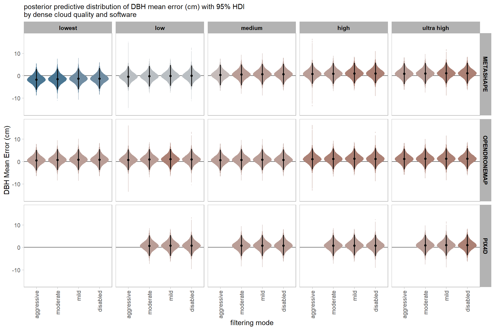
and a table of these 95% HDI values
table_temp =
  fltr_sftwr_draws_temp %>%
  tidybayes::median_hdi(value) %>%
  dplyr::inner_join(
    ptcld_validation_data %>% dplyr::distinct(software, depth_maps_generation_quality, depth_maps_generation_filtering_mode)
    , by = dplyr::join_by(software, depth_maps_generation_quality, depth_maps_generation_filtering_mode)
  ) %>%
  dplyr::mutate(depth_maps_generation_quality = depth_maps_generation_quality %>% forcats::fct_rev()) %>%
  dplyr::select(c(
    software, depth_maps_generation_quality, depth_maps_generation_filtering_mode
    , value, .lower, .upper
  )) %>%
  dplyr::ungroup() %>%
  dplyr::arrange(software, depth_maps_generation_quality, depth_maps_generation_filtering_mode)

table_temp %>%
  # dplyr::select(-c(software)) %>%
  kableExtra::kbl(
    digits = 2
    , caption = "DBH Mean Error (cm)<br>95% HDI of the posterior predictive distribution"
    , col.names = c(
      "software", "quality", "filtering mode"
      , "DBH Mean Error (cm)<br>median"
      , "HDI low", "HDI high"
    )
    , escape = F
  ) %>%
  kableExtra::kable_styling() %>%
  # kableExtra::pack_rows(index = table(forcats::fct_inorder(table_temp$software))) %>%
  kableExtra::collapse_rows(columns = 1:2, valign = "top") %>%
kableExtra::scroll_box(height = "8in")| software | quality | filtering mode |
DBH Mean Error (cm) median |
HDI low | HDI high |
|---|---|---|---|---|---|
| METASHAPE | lowest | aggressive | -1.74 | -6.24 | 2.98 |
| moderate | -1.50 | -6.10 | 3.10 | ||
| mild | -1.27 | -6.03 | 3.17 | ||
| disabled | -1.28 | -5.85 | 3.36 | ||
| low | aggressive | -0.43 | -5.02 | 4.15 | |
| moderate | -0.26 | -4.86 | 4.30 | ||
| mild | -0.07 | -4.47 | 4.70 | ||
| disabled | -0.05 | -4.68 | 4.51 | ||
| medium | aggressive | 0.36 | -4.32 | 4.86 | |
| moderate | 0.54 | -4.28 | 4.92 | ||
| mild | 0.68 | -3.99 | 5.19 | ||
| disabled | 0.67 | -3.93 | 5.24 | ||
| high | aggressive | 0.81 | -3.66 | 5.54 | |
| moderate | 0.92 | -3.60 | 5.55 | ||
| mild | 1.03 | -3.43 | 5.72 | ||
| disabled | 1.03 | -3.44 | 5.72 | ||
| ultra high | aggressive | 0.87 | -3.72 | 5.43 | |
| moderate | 0.98 | -3.63 | 5.57 | ||
| mild | 1.09 | -3.39 | 5.78 | ||
| disabled | 1.09 | -3.55 | 5.65 | ||
| OPENDRONEMAP | lowest | aggressive | 0.57 | -4.01 | 5.15 |
| moderate | 0.78 | -3.73 | 5.45 | ||
| mild | 0.88 | -3.74 | 5.40 | ||
| disabled | 0.82 | -3.76 | 5.42 | ||
| low | aggressive | 0.74 | -3.88 | 5.30 | |
| moderate | 0.92 | -3.68 | 5.48 | ||
| mild | 1.02 | -3.57 | 5.57 | ||
| disabled | 0.96 | -3.63 | 5.54 | ||
| medium | aggressive | 0.61 | -3.96 | 5.22 | |
| moderate | 0.79 | -3.77 | 5.42 | ||
| mild | 0.87 | -3.77 | 5.39 | ||
| disabled | 0.78 | -3.80 | 5.39 | ||
| high | aggressive | 1.08 | -3.45 | 5.78 | |
| moderate | 1.18 | -3.37 | 5.77 | ||
| mild | 1.24 | -3.46 | 5.73 | ||
| disabled | 1.21 | -3.34 | 5.88 | ||
| ultra high | aggressive | 1.13 | -3.45 | 5.72 | |
| moderate | 1.25 | -3.35 | 5.83 | ||
| mild | 1.31 | -3.42 | 5.75 | ||
| disabled | 1.24 | -3.33 | 5.85 | ||
| PIX4D | low | moderate | 0.75 | -3.82 | 5.33 |
| mild | 0.81 | -3.73 | 5.43 | ||
| disabled | 0.83 | -3.80 | 5.38 | ||
| medium | moderate | 0.81 | -3.78 | 5.43 | |
| mild | 0.87 | -3.78 | 5.43 | ||
| disabled | 0.84 | -3.60 | 5.58 | ||
| high | moderate | 0.84 | -3.75 | 5.47 | |
| mild | 0.86 | -3.53 | 5.69 | ||
| disabled | 0.87 | -3.74 | 5.49 | ||
| ultra high | moderate | 0.97 | -3.61 | 5.58 | |
| mild | 0.99 | -3.70 | 5.45 | ||
| disabled | 1.00 | -3.45 | 5.70 |
7.4.3 Model: DBH RMSE (precision)
Define priors
# from Kurz:
gamma_a_b_from_omega_sigma = function(mode, sd) {
  if (mode <= 0) stop("mode must be > 0")
  if (sd   <= 0) stop("sd must be > 0")
  rate = (mode + sqrt(mode^2 + 4 * sd^2)) / (2 * sd^2)
  shape = 1 + mode * rate
  return(list(shape = shape, rate = rate))
}

mean_y_temp = mean(ptcld_validation_data$dbh_cm_rmse, na.rm = T)
sd_y_temp   = sd(ptcld_validation_data$dbh_cm_rmse, na.rm = T)

omega_temp = sd_y_temp / 2
sigma_temp = 2 * sd_y_temp

s_r_temp = gamma_a_b_from_omega_sigma(mode = omega_temp, sd = sigma_temp)

stanvars_temp =
  brms::stanvar(mean_y_temp,    name = "mean_y") +
  brms::stanvar(sd_y_temp,      name = "sd_y") +
  brms::stanvar(s_r_temp$shape, name = "alpha") +
  brms::stanvar(s_r_temp$rate,  name = "beta")
7.4.3.1 Prior distributions
#### setting priors
# required libraries: tidyverse, tidybayes, brms, palettetown, latex2exp
priors_temp <- c(
    brms::prior(normal(mean_y_temp, sd_y_temp * 5), class = "Intercept")
    , brms::prior(gamma(s_r_temp$shape, s_r_temp$rate), class = "sd")
    , brms::prior(cauchy(0, sd_y_temp), class = "sigma")
  )
# plot
plt_prior4 =
priors_temp %>%
  tidybayes::parse_dist() %>%
  tidybayes::marginalize_lkjcorr(K = 2) %>%
  tidyr::separate(
    .args
    , sep = ","
    , into = c("a","b")
    , remove = F
  ) %>%
  dplyr::mutate(
    distrib = paste0(
      class, " ~ "
      , .dist
      , "("
      , a %>% readr::parse_number() %>% round(2)
      , ","
      , b %>% readr::parse_number() %>% round(2)
      , ")"
    )
  ) %>%
  ggplot(., aes(dist = .dist, args = .args)) +
  facet_grid(cols=vars(distrib), scales = "free") +
  ggdist::stat_halfeye(
    aes(fill = prior),
    n = 10e2,
    show.legend = F
    , fill = "slategray"
  ) +
  coord_flip() +
  theme_light() +
  theme(
    strip.text = element_text(face = "bold", color = "black"),
    axis.text.y = element_blank(),
    axis.ticks = element_blank()
    , axis.text = element_text(size = 6)
  )+
  labs(
    x = ""
    , title = "Priors: DBH RMSE (precision)"
    , y = ""
  )
plt_prior4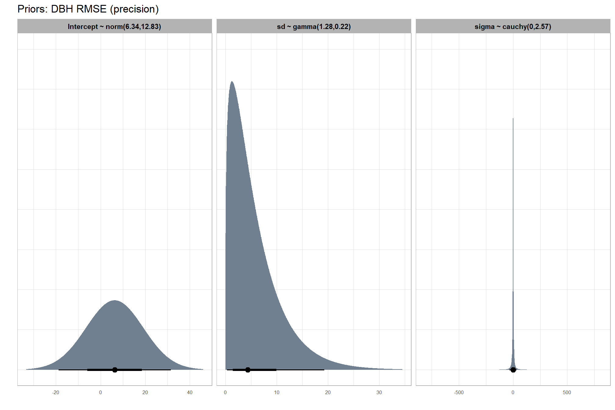
7.4.3.2 Fit the model
Now fit the model.
brms_dbh_rmse_mod = brms::brm(
  formula = dbh_cm_rmse ~
    # baseline
    1 +
    # main effects
    (1 | depth_maps_generation_quality) +
    (1 | depth_maps_generation_filtering_mode) +
    (1 | software) +
    (1 | study_site) + # only fitting main effects of site and not interactions
    # two-way interactions
    (1 | depth_maps_generation_quality:depth_maps_generation_filtering_mode) +
    (1 | depth_maps_generation_quality:software) +
    (1 | depth_maps_generation_filtering_mode:software) +
    # three-way interactions
    (1 | depth_maps_generation_quality:depth_maps_generation_filtering_mode:software)
  , data = ptcld_validation_data
  , family = brms::brmsfamily(family = "gaussian")
  , iter = 20000, warmup = 10000, chains = 4
  , control = list(adapt_delta = 0.999, max_treedepth = 13)
  , cores = round(parallel::detectCores()/2)
  , prior = c(
    brms::prior(normal(mean_y, sd_y * 5), class = "Intercept")
    , brms::prior(gamma(alpha, beta), class = "sd")
    , brms::prior(cauchy(0, sd_y), class = "sigma")
  )
  , stanvars = stanvars_temp
  , file = paste0(rootdir, "/fits/brms_dbh_rmse_mod")
)
7.4.3.3 Quality:Filtering - interaction
draws_temp =
  ptcld_validation_data %>%
    dplyr::distinct(depth_maps_generation_quality, depth_maps_generation_filtering_mode) %>%
    tidybayes::add_epred_draws(
      brms_dbh_rmse_mod, allow_new_levels = T
      # this part is crucial
      , re_formula = ~ (1 | depth_maps_generation_quality) +
        (1 | depth_maps_generation_filtering_mode) +
        (1 | depth_maps_generation_quality:depth_maps_generation_filtering_mode)
    ) %>%
    dplyr::rename(value = .epred) %>%
    dplyr::mutate(med = tidybayes::median_hdci(value)$y)
# plot
  draws_temp %>%
    dplyr::mutate(depth_maps_generation_quality = depth_maps_generation_quality %>% forcats::fct_rev()) %>%
  # plot
  ggplot(
    mapping = aes(
      y = value, x = depth_maps_generation_filtering_mode
      , fill = med
    )
  ) +
    geom_hline(yintercept = 0, color = "gray33") +
    tidybayes::stat_eye(
      point_interval = median_hdi, .width = .95
      , slab_alpha = 0.98
      , interval_color = "black", linewidth = 1
      , point_color = "black", point_fill = "black", point_size = 1
    ) +
    scale_fill_stepsn(
      n.breaks = 5
      , colors = viridis::mako(n = 5, begin = 0.2, end = 0.9, direction = -1)
      , limits = c(0,lmt_dbh_cm_rmse)
      , labels = scales::comma_format(accuracy = 0.01)
      , show.limits = T
    ) +
    facet_grid(cols = vars(depth_maps_generation_quality)) +
    scale_y_continuous(limits = c(-0.02,NA)) +
    labs(
      x = "filtering mode", y = "DBH RMSE (cm)"
      , subtitle = "posterior predictive distribution of DBH RMSE (cm) with 95% HDI\nby dense cloud quality"
    ) +
    theme_light() +
    theme(
      legend.position = "none"
      , legend.direction  = "horizontal"
      , axis.text.x = element_text(angle = 90, vjust = 0.5, hjust = 1)
      , strip.text = element_text(color = "black", face = "bold")
) 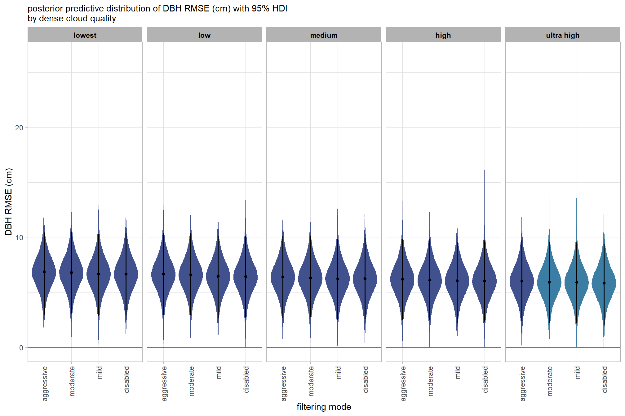
and a table of these 95% HDI values
table_temp =
  draws_temp %>%
    tidybayes::median_hdi(value) %>%
    dplyr::select(-c(.point,.interval, .width,.row)) %>%
    dplyr::arrange(depth_maps_generation_quality,depth_maps_generation_filtering_mode)

table_temp %>%
  dplyr::select(-c(depth_maps_generation_quality)) %>%
  kableExtra::kbl(
    digits = 2
    , caption = "DBH RMSE (cm)<br>95% HDI of the posterior predictive distribution"
    , col.names = c(
      "filtering mode"
      , "DBH RMSE (cm)<br>median"
      , "HDI low", "HDI high"
    )
    , escape = F
  ) %>%
  kableExtra::kable_styling() %>%
  kableExtra::pack_rows(index = table(forcats::fct_inorder(table_temp$depth_maps_generation_quality))) %>%
kableExtra::scroll_box(height = "8in")| filtering mode |
DBH RMSE (cm) median |
HDI low | HDI high |
|---|---|---|---|
| ultra high | |||
| aggressive | 6.00 | 2.19 | 9.79 |
| moderate | 5.93 | 2.11 | 9.71 |
| mild | 5.88 | 2.04 | 9.66 |
| disabled | 5.85 | 2.11 | 9.72 |
| high | |||
| aggressive | 6.19 | 2.43 | 10.00 |
| moderate | 6.10 | 2.21 | 9.81 |
| mild | 6.05 | 2.21 | 9.79 |
| disabled | 6.04 | 2.19 | 9.78 |
| medium | |||
| aggressive | 6.39 | 2.65 | 10.25 |
| moderate | 6.31 | 2.53 | 10.13 |
| mild | 6.23 | 2.47 | 10.07 |
| disabled | 6.23 | 2.43 | 10.04 |
| low | |||
| aggressive | 6.64 | 2.81 | 10.43 |
| moderate | 6.59 | 2.75 | 10.36 |
| mild | 6.45 | 2.69 | 10.31 |
| disabled | 6.44 | 2.62 | 10.24 |
| lowest | |||
| aggressive | 6.85 | 2.93 | 10.55 |
| moderate | 6.79 | 2.95 | 10.54 |
| mild | 6.66 | 2.82 | 10.44 |
| disabled | 6.67 | 2.81 | 10.44 |
we can also make pairwise comparisons
# make the contrasts using compare_levels
brms_contrast_temp = draws_temp %>%
    tidybayes::compare_levels(
      value
      , by = depth_maps_generation_quality
      , comparison =
        contrast_list
        # tidybayes::emmeans_comparison("revpairwise")
        #"pairwise"
    ) %>%
    dplyr::rename(contrast = depth_maps_generation_quality)

# separate contrast
brms_contrast_temp = brms_contrast_temp %>%
  dplyr::ungroup() %>%
  tidyr::separate_wider_delim(
    cols = contrast
    , delim = " - "
    , names = paste0(
        "sorter"
        , 1:(max(stringr::str_count(brms_contrast_temp$contrast, "-"))+1)
      )
    , too_few = "align_start"
    , cols_remove = F
  ) %>%
  dplyr::filter(sorter1!=sorter2) %>%
  dplyr::mutate(
    dplyr::across(
      tidyselect::starts_with("sorter")
      , .fns = function(x){factor(
        x, ordered = T
        , levels = levels(ptcld_validation_data$depth_maps_generation_quality)
      )}
    )
    , contrast = contrast %>%
      forcats::fct_reorder(
        paste0(as.numeric(sorter1), as.numeric(sorter2)) %>%
        as.numeric()
      )
    , depth_maps_generation_filtering_mode = depth_maps_generation_filtering_mode %>%
      factor(
        levels = levels(ptcld_validation_data$depth_maps_generation_filtering_mode)
        , ordered = T
      )
  ) %>%
  # median_hdi summary for coloring
  dplyr::group_by(contrast,depth_maps_generation_filtering_mode) %>%
  make_contrast_vars()
plot it
plt_contrast(
  brms_contrast_temp
  # , caption_text = form_temp
  , y_axis_title = "quality"
  , facet = "depth_maps_generation_filtering_mode"
  , label_size = 1.7
  , x_expand = c(0.2,0.05)
) +
  labs(
    subtitle = "posterior predictive distribution of group constrasts with 95% & 50% HDI\nby filtering mode"
    , x = "constrast DBH RMSE (cm)"
  ) +
  theme(
    axis.text.x = element_text(size = 7)
  )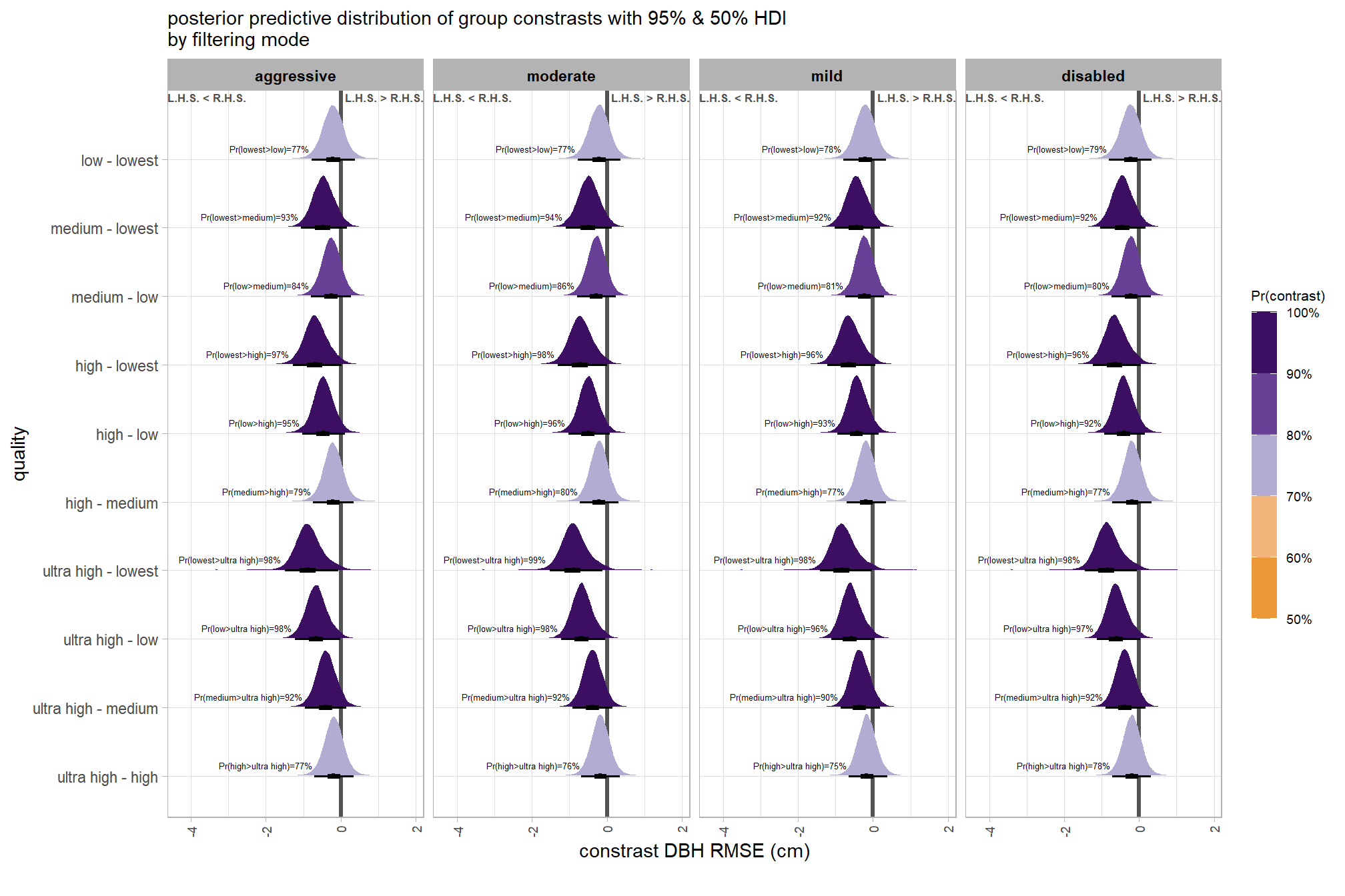
ggplot2::ggsave(
  "../data/qlty_fltr_comp_dbh_rmse.png"
  , plot = ggplot2::last_plot() + labs(subtitle = "")
  , height = 7, width = 10.5
)
and summarize these contrasts
brms_contrast_temp %>%
  dplyr::group_by(contrast, depth_maps_generation_filtering_mode, pr_lt_zero) %>%
  tidybayes::median_hdi(value) %>%
  dplyr::arrange(contrast, depth_maps_generation_filtering_mode) %>%
  dplyr::select(contrast, depth_maps_generation_filtering_mode, value, .lower, .upper, pr_lt_zero) %>%

kableExtra::kbl(
    digits = 2
    , caption = "DBH RMSE (cm)<br>95% HDI of the posterior predictive distribution of group contrasts"
    , col.names = c(
      "quality contrast"
      , "filtering mode"
      , "median difference<br>DBH RMSE (cm)"
      , "HDI low", "HDI high"
      , "Pr(diff<0)"
    )
    , escape = F
  ) %>%
  kableExtra::kable_styling() %>%
kableExtra::scroll_box(height = "8in")| quality contrast | filtering mode |
median difference DBH RMSE (cm) |
HDI low | HDI high | Pr(diff<0) |
|---|---|---|---|---|---|
| ultra high - high | aggressive | -0.18 | -0.72 | 0.35 | 77% |
| ultra high - high | moderate | -0.17 | -0.68 | 0.34 | 76% |
| ultra high - high | mild | -0.16 | -0.65 | 0.39 | 75% |
| ultra high - high | disabled | -0.19 | -0.71 | 0.32 | 78% |
| ultra high - medium | aggressive | -0.39 | -0.95 | 0.14 | 92% |
| ultra high - medium | moderate | -0.38 | -0.92 | 0.15 | 92% |
| ultra high - medium | mild | -0.35 | -0.87 | 0.19 | 90% |
| ultra high - medium | disabled | -0.38 | -0.90 | 0.17 | 92% |
| ultra high - low | aggressive | -0.65 | -1.22 | -0.01 | 98% |
| ultra high - low | moderate | -0.66 | -1.22 | -0.05 | 98% |
| ultra high - low | mild | -0.59 | -1.12 | 0.04 | 96% |
| ultra high - low | disabled | -0.60 | -1.13 | 0.03 | 97% |
| ultra high - lowest | aggressive | -0.87 | -1.49 | -0.07 | 98% |
| ultra high - lowest | moderate | -0.88 | -1.52 | -0.11 | 99% |
| ultra high - lowest | mild | -0.80 | -1.42 | -0.02 | 98% |
| ultra high - lowest | disabled | -0.84 | -1.46 | -0.06 | 98% |
| high - medium | aggressive | -0.21 | -0.74 | 0.34 | 79% |
| high - medium | moderate | -0.21 | -0.72 | 0.31 | 80% |
| high - medium | mild | -0.19 | -0.70 | 0.34 | 77% |
| high - medium | disabled | -0.19 | -0.71 | 0.33 | 77% |
| high - low | aggressive | -0.46 | -1.03 | 0.11 | 95% |
| high - low | moderate | -0.49 | -1.03 | 0.07 | 96% |
| high - low | mild | -0.42 | -0.94 | 0.15 | 93% |
| high - low | disabled | -0.40 | -0.94 | 0.16 | 92% |
| high - lowest | aggressive | -0.68 | -1.28 | 0.02 | 97% |
| high - lowest | moderate | -0.70 | -1.31 | 0.00 | 98% |
| high - lowest | mild | -0.63 | -1.23 | 0.07 | 96% |
| high - lowest | disabled | -0.64 | -1.24 | 0.05 | 96% |
| medium - low | aggressive | -0.25 | -0.80 | 0.28 | 84% |
| medium - low | moderate | -0.27 | -0.80 | 0.24 | 86% |
| medium - low | mild | -0.23 | -0.74 | 0.29 | 81% |
| medium - low | disabled | -0.21 | -0.73 | 0.31 | 80% |
| medium - lowest | aggressive | -0.46 | -1.06 | 0.16 | 93% |
| medium - lowest | moderate | -0.48 | -1.10 | 0.13 | 94% |
| medium - lowest | mild | -0.44 | -1.03 | 0.18 | 92% |
| medium - lowest | disabled | -0.44 | -1.04 | 0.17 | 92% |
| low - lowest | aggressive | -0.21 | -0.78 | 0.38 | 77% |
| low - lowest | moderate | -0.20 | -0.78 | 0.37 | 77% |
| low - lowest | mild | -0.21 | -0.79 | 0.36 | 78% |
| low - lowest | disabled | -0.23 | -0.80 | 0.34 | 79% |
7.4.3.4 Software:Quality - interaction
draws_temp =
  tidyr::crossing(
    depth_maps_generation_quality = unique(ptcld_validation_data$depth_maps_generation_quality)
    , software = unique(ptcld_validation_data$software)
  ) %>%
    tidybayes::add_epred_draws(
      brms_dbh_rmse_mod, allow_new_levels = T
      # this part is crucial
      , re_formula = ~ (1 | depth_maps_generation_quality) +
        (1 | software) +
        (1 | depth_maps_generation_quality:software)
    ) %>%
    dplyr::rename(value = .epred) %>%
    dplyr::mutate(med = tidybayes::median_hdci(value)$y)
# plot
  draws_temp %>%
    # remove out-of-sample obs
    dplyr::inner_join(
      ptcld_validation_data %>% dplyr::distinct(depth_maps_generation_quality, software)
      , by = dplyr::join_by(depth_maps_generation_quality, software)
    ) %>%
    dplyr::mutate(depth_maps_generation_quality = depth_maps_generation_quality %>% forcats::fct_rev()) %>%
  # plot
  ggplot(
    mapping = aes(
      y = value, x = software
      , fill = med
    )
  ) +
    geom_hline(yintercept = 0, color = "gray33") +
    tidybayes::stat_eye(
      point_interval = median_hdi, .width = .95
      , slab_alpha = 0.98
      , interval_color = "black", linewidth = 1
      , point_color = "black", point_fill = "black", point_size = 1
    ) +
    scale_fill_stepsn(
      n.breaks = 5
      , colors = viridis::mako(n = 5, begin = 0.2, end = 0.9, direction = -1)
      , limits = c(0,lmt_dbh_cm_rmse)
      , labels = scales::comma_format(accuracy = 0.01)
      , show.limits = T
    ) +
    facet_grid(cols = vars(depth_maps_generation_quality)) +
    scale_y_continuous(limits = c(-0.02,NA)) +
    labs(
      x = "software", y = "DBH RMSE (cm)"
      , subtitle = "posterior predictive distribution of DBH RMSE (cm) with 95% HDI\nby dense cloud quality"
    ) +
    theme_light() +
    theme(
      legend.position = "none"
      , legend.direction  = "horizontal"
      , axis.text.x = element_text(angle = 90, vjust = 0.5, hjust = 1)
      , strip.text = element_text(color = "black", face = "bold")
) 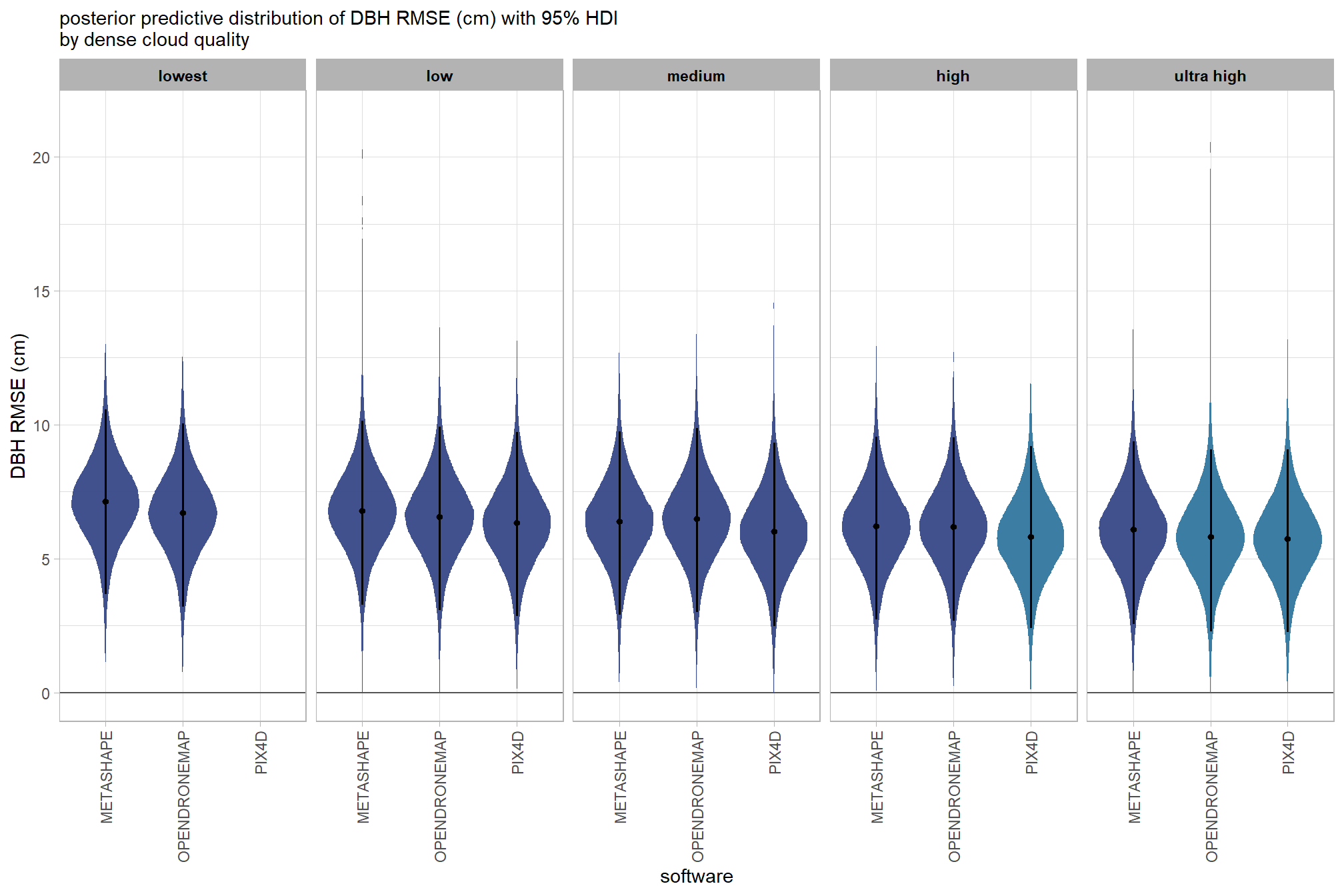
and a table of these 95% HDI values
table_temp =
  draws_temp %>%
  tidybayes::median_hdi(value) %>%
  # remove out-of-sample obs
    dplyr::inner_join(
      ptcld_validation_data %>% dplyr::distinct(depth_maps_generation_quality, software)
      , by = dplyr::join_by(depth_maps_generation_quality, software)
    ) %>%
  dplyr::select(-c(.point,.interval, .width,.row)) %>%
  dplyr::arrange(software,depth_maps_generation_quality)

table_temp %>%
  dplyr::select(-c(software)) %>%
  kableExtra::kbl(
    digits = 2
    , caption = "DBH RMSE (cm)<br>95% HDI of the posterior predictive distribution"
    , col.names = c(
      "quality"
      , "DBH RMSE (cm)<br>median"
      , "HDI low", "HDI high"
    )
    , escape = F
  ) %>%
  kableExtra::kable_styling() %>%
  kableExtra::pack_rows(index = table(forcats::fct_inorder(table_temp$software))) %>%
kableExtra::scroll_box(height = "8in")| quality |
DBH RMSE (cm) median |
HDI low | HDI high |
|---|---|---|---|
| METASHAPE | |||
| ultra high | 6.07 | 2.54 | 9.49 |
| high | 6.21 | 2.61 | 9.54 |
| medium | 6.39 | 2.99 | 9.91 |
| low | 6.78 | 3.27 | 10.22 |
| lowest | 7.14 | 3.65 | 10.59 |
| OPENDRONEMAP | |||
| ultra high | 5.81 | 2.28 | 9.23 |
| high | 6.19 | 2.62 | 9.56 |
| medium | 6.47 | 2.93 | 9.88 |
| low | 6.57 | 3.03 | 9.97 |
| lowest | 6.70 | 3.16 | 10.10 |
| PIX4D | |||
| ultra high | 5.74 | 2.30 | 9.27 |
| high | 5.81 | 2.29 | 9.24 |
| medium | 6.00 | 2.44 | 9.38 |
| low | 6.32 | 2.77 | 9.73 |
we can also make pairwise comparisons
# calculate contrast
brms_contrast_temp = draws_temp %>%
  tidybayes::compare_levels(
    value
    , by = depth_maps_generation_quality
    , comparison = contrast_list
  ) %>%
  dplyr::rename(contrast = depth_maps_generation_quality)

# separate contrast
brms_contrast_temp = brms_contrast_temp %>%
  dplyr::ungroup() %>%
  tidyr::separate_wider_delim(
    cols = contrast
    , delim = " - "
    , names = paste0(
      "sorter"
      , 1:(max(stringr::str_count(brms_contrast_temp$contrast, "-"))+1)
    )
    , too_few = "align_start"
    , cols_remove = F
  ) %>%
  dplyr::filter(sorter1!=sorter2) %>%
  dplyr::mutate(
    dplyr::across(
      tidyselect::starts_with("sorter")
      , .fns = function(x){factor(
        x, ordered = T
        , levels = levels(ptcld_validation_data$depth_maps_generation_quality)
      )}
    )
    , contrast = contrast %>%
      forcats::fct_reorder(
        paste0(as.numeric(sorter1), as.numeric(sorter2)) %>%
          as.numeric()
      )
  ) %>%
  # median_hdi summary for coloring
  dplyr::group_by(contrast, software) %>%
  make_contrast_vars()

# remove out-of-sample obs
brms_contrast_temp = brms_contrast_temp %>%
  dplyr::inner_join(
    ptcld_validation_data %>% dplyr::distinct(software, depth_maps_generation_quality)
    , by = dplyr::join_by(software, sorter1 == depth_maps_generation_quality)
  ) %>%
  dplyr::inner_join(
    ptcld_validation_data %>% dplyr::distinct(software, depth_maps_generation_quality)
    , by = dplyr::join_by(software, sorter2 == depth_maps_generation_quality)
  )
plot it
plt_contrast(
  brms_contrast_temp
  # , caption_text = form_temp
  , y_axis_title = "quality"
  , facet = "software"
  , label_size = 1.8
  , x_expand = c(0.33,0.05)
) +
  labs(
    subtitle = "posterior predictive distribution of group constrasts with 95% & 50% HDI\nby software"
    , x = "constrast DBH RMSE (cm)"
  )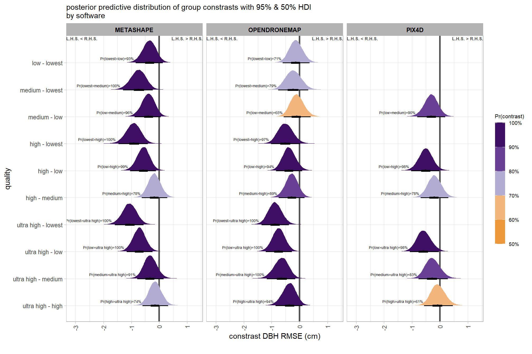
ggplot2::ggsave(
  "../data/qlty_sftwr_comp_dbh_rmse.png"
  , plot = ggplot2::last_plot() + labs(subtitle = "")
  , height = 7, width = 10.5
)
create plot for combining with other RMSE contrasts for publication
ptchwrk_qlty_sftwr_comp_dbh_rmse =
  plt_contrast(
    brms_contrast_temp
    , y_axis_title = "quality contrast"
    , facet = "software"
    , label_size = 1.5
    , label = "pr_diff_lab_sm"
    , annotate_size = 1.8
  ) +
    labs(
      subtitle = "" # "constrast Height RMSE (m)"
      , x = "DBH RMSE (cm) constrast"
    ) +
    theme(
      legend.position="none"
      , axis.title.y = element_text(size = 10, face = "bold")
      , axis.title.x = element_text(size = 8)
    )
# ptchwrk_qlty_sftwr_comp_dbh_rmse
and summarize these contrasts
table_temp = brms_contrast_temp %>%
  dplyr::group_by(contrast, software, pr_lt_zero) %>%
  tidybayes::median_hdi(value) %>%
  dplyr::arrange(contrast, software) %>%
  dplyr::select(contrast, software, value, .lower, .upper, pr_lt_zero) %>%
  dplyr::arrange(software, contrast)

table_temp %>%
  dplyr::select(-c(software)) %>%
  kableExtra::kbl(
    digits = 1
    , caption = "DBH RMSE (cm)<br>95% HDI of the posterior predictive distribution of group contrasts"
    , col.names = c(
      "quality contrast"
      , "median difference<br>DBH RMSE (cm)"
      , "HDI low", "HDI high"
      , "Pr(diff<0)"
    )
    , escape = F
  ) %>%
  kableExtra::kable_styling() %>%
  kableExtra::pack_rows(index = table(forcats::fct_inorder(table_temp$software))) %>%
kableExtra::scroll_box(height = "8in")| quality contrast |
median difference DBH RMSE (cm) |
HDI low | HDI high | Pr(diff<0) |
|---|---|---|---|---|
| METASHAPE | ||||
| ultra high - high | -0.1 | -0.6 | 0.3 | 74% |
| ultra high - medium | -0.3 | -0.8 | 0.2 | 91% |
| ultra high - low | -0.7 | -1.2 | -0.2 | 100% |
| ultra high - lowest | -1.1 | -1.6 | -0.6 | 100% |
| high - medium | -0.2 | -0.6 | 0.3 | 78% |
| high - low | -0.6 | -1.0 | -0.1 | 99% |
| high - lowest | -0.9 | -1.5 | -0.4 | 100% |
| medium - low | -0.4 | -0.9 | 0.1 | 96% |
| medium - lowest | -0.7 | -1.3 | -0.2 | 100% |
| low - lowest | -0.4 | -0.8 | 0.1 | 93% |
| OPENDRONEMAP | ||||
| ultra high - high | -0.4 | -0.9 | 0.1 | 94% |
| ultra high - medium | -0.6 | -1.2 | -0.2 | 100% |
| ultra high - low | -0.7 | -1.2 | -0.3 | 100% |
| ultra high - lowest | -0.9 | -1.4 | -0.4 | 100% |
| high - medium | -0.3 | -0.8 | 0.2 | 89% |
| high - low | -0.4 | -0.8 | 0.1 | 94% |
| high - lowest | -0.5 | -1.0 | 0.0 | 97% |
| medium - low | -0.1 | -0.6 | 0.4 | 65% |
| medium - lowest | -0.2 | -0.8 | 0.3 | 79% |
| low - lowest | -0.1 | -0.6 | 0.4 | 71% |
| PIX4D | ||||
| ultra high - high | -0.1 | -0.6 | 0.5 | 61% |
| ultra high - medium | -0.3 | -0.8 | 0.3 | 83% |
| ultra high - low | -0.6 | -1.1 | 0.0 | 98% |
| high - medium | -0.2 | -0.7 | 0.3 | 78% |
| high - low | -0.5 | -1.0 | 0.0 | 98% |
| medium - low | -0.3 | -0.8 | 0.2 | 90% |
The contrasts above address the question “are there differences in RMSE based on dense point cloud generation quality within each software?”.
To address the different question of “are there differences in RMSE based on the processing software used at a given dense point cloud generation quality?” we need to utilize a different formulation of the comparison parameter within our call to the tidybayes::compare_levels function and calculate the contrast by software instead
# calculate contrast
brms_contrast_temp = draws_temp %>%
  tidybayes::compare_levels(
    value
    , by = software
    , comparison = "pairwise"
  ) %>%
  dplyr::rename(contrast = software) %>%
  # median_hdi summary for coloring
  dplyr::group_by(contrast, depth_maps_generation_quality) %>%
  make_contrast_vars()

# remove out-of-sample obs
brms_contrast_temp = brms_contrast_temp %>%
  tidyr::separate_wider_delim(
    cols = contrast
    , delim = " - "
    , names = paste0(
      "sorter"
      , 1:(max(stringr::str_count(brms_contrast_temp$contrast, "-"))+1)
    )
    , too_few = "align_start"
    , cols_remove = F
  ) %>%
  dplyr::filter(sorter1!=sorter2) %>%
  dplyr::inner_join(
    ptcld_validation_data %>% dplyr::distinct(software, depth_maps_generation_quality)
    , by = dplyr::join_by(sorter1 == software, depth_maps_generation_quality)
  ) %>%
  dplyr::inner_join(
    ptcld_validation_data %>% dplyr::distinct(software, depth_maps_generation_quality)
    , by = dplyr::join_by(sorter2 == software, depth_maps_generation_quality)
  )
plot it
plt_contrast(
  brms_contrast_temp
  # , caption_text = form_temp
  , y_axis_title = "software"
  , facet = "depth_maps_generation_quality"
  , label_size = 1.9
  # , x_expand = c(0.25,0.1)
) +
  facet_wrap(facets = vars(depth_maps_generation_quality), ncol = 2) +
  labs(
    subtitle = "posterior predictive distribution of group constrasts with 95% & 50% HDI\nby dense cloud quality"
    , x = "constrast DBH RMSE (cm)"
  ) +
  theme(
    legend.position = c(.75, .13)
  ) +
  guides(fill = guide_colorbar(theme = theme(
    legend.key.width  = unit(1, "lines"),
    legend.key.height = unit(7, "lines")
  )))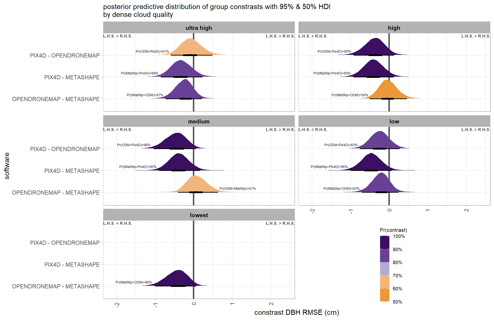
ggplot2::ggsave(
  "../data/sftwr_qlty_comp_dbh_rmse.png"
  , plot = ggplot2::last_plot() + labs(subtitle = "")
  , height = 7, width = 10.5
)
create plot for combining with other RMSE contrasts for publication
ptchwrk_sftwr_qlty_comp_dbh_rmse =
  plt_contrast(
    brms_contrast_temp
    , y_axis_title = "software contrast"
    , facet = "depth_maps_generation_quality"
    , label_size = 1.7
    , label = "pr_diff_lab_sm"
    , annotate_size = 1.8
  ) +
    facet_wrap(facets = vars(depth_maps_generation_quality), ncol = 3) +
    labs(
      subtitle = ""
      , x = "DBH RMSE (cm) constrast"
    ) +
    theme(
      legend.position = "inside"
      , legend.position.inside = c(.8, .13)
      , axis.title.y = element_text(size = 10, face = "bold")
      , axis.title.x = element_text(size = 8)
    ) +
    guides(fill = guide_colorbar(theme = theme(
      legend.key.width  = unit(1, "lines"),
      legend.key.height = unit(6.5, "lines")
    )))
# ptchwrk_sftwr_qlty_comp_dbh_rmse
and summarize these contrasts
table_temp = brms_contrast_temp %>%
  dplyr::group_by(contrast, depth_maps_generation_quality, pr_lt_zero) %>%
  tidybayes::median_hdi(value) %>%
  dplyr::arrange(contrast, depth_maps_generation_quality) %>%
  dplyr::select(contrast, depth_maps_generation_quality, value, .lower, .upper, pr_lt_zero)

table_temp %>%
  dplyr::select(-c(contrast)) %>%
  kableExtra::kbl(
    digits = 1
    , caption = "DBH RMSE (cm)<br>95% HDI of the posterior predictive distribution of group contrasts"
    , col.names = c(
      "quality contrast"
      , "median difference<br>DBH RMSE (cm)"
      , "HDI low", "HDI high"
      , "Pr(diff<0)"
    )
    , escape = F
  ) %>%
  kableExtra::kable_styling() %>%
  kableExtra::pack_rows(index = table(forcats::fct_inorder(table_temp$contrast))) %>%
kableExtra::scroll_box(height = "8in")| quality contrast |
median difference DBH RMSE (cm) |
HDI low | HDI high | Pr(diff<0) |
|---|---|---|---|---|
| OPENDRONEMAP - METASHAPE | ||||
| ultra high | -0.2 | -0.7 | 0.2 | 87% |
| high | 0.0 | -0.5 | 0.5 | 56% |
| medium | 0.1 | -0.4 | 0.6 | 39% |
| low | -0.2 | -0.7 | 0.2 | 83% |
| lowest | -0.4 | -1.0 | 0.1 | 96% |
| PIX4D - METASHAPE | ||||
| ultra high | -0.3 | -0.9 | 0.2 | 88% |
| high | -0.4 | -0.9 | 0.1 | 93% |
| medium | -0.4 | -0.9 | 0.2 | 92% |
| low | -0.5 | -1.0 | 0.1 | 96% |
| PIX4D - OPENDRONEMAP | ||||
| ultra high | -0.1 | -0.6 | 0.5 | 61% |
| high | -0.4 | -0.9 | 0.1 | 93% |
| medium | -0.5 | -1.0 | 0.1 | 96% |
| low | -0.2 | -0.8 | 0.3 | 83% |
7.4.3.5 Software:Filtering - interaction
draws_temp =
  tidyr::crossing(
      depth_maps_generation_filtering_mode = unique(ptcld_validation_data$depth_maps_generation_filtering_mode)
      , software = unique(ptcld_validation_data$software)
    ) %>%
    tidybayes::add_epred_draws(
      brms_dbh_rmse_mod, allow_new_levels = T
      # this part is crucial
      , re_formula = ~ (1 | depth_maps_generation_filtering_mode) +
        (1 | software) +
        (1 | depth_maps_generation_filtering_mode:software)
    ) %>%
    dplyr::rename(value = .epred) %>%
    dplyr::mutate(med = tidybayes::median_hdci(value)$y)
# plot
  draws_temp %>%
  # remove out-of-sample obs
  dplyr::inner_join(
    ptcld_validation_data %>% dplyr::distinct(depth_maps_generation_filtering_mode, software)
    , by = dplyr::join_by(depth_maps_generation_filtering_mode, software)
  ) %>%
  # plot
  ggplot(
    mapping = aes(
      y = value, x = software
      , fill = med
    )
  ) +
    geom_hline(yintercept = 0, color = "gray33") +
    tidybayes::stat_eye(
      point_interval = median_hdi, .width = .95
      , slab_alpha = 0.98
      , interval_color = "black", linewidth = 1
      , point_color = "black", point_fill = "black", point_size = 1
    ) +
    scale_fill_stepsn(
      n.breaks = 5
      , colors = viridis::mako(n = 5, begin = 0.2, end = 0.9, direction = -1)
      , limits = c(0,lmt_dbh_cm_rmse)
      , labels = scales::comma_format(accuracy = 0.01)
      , show.limits = T
    ) +
    facet_grid(cols = vars(depth_maps_generation_filtering_mode)) +
    scale_y_continuous(limits = c(-0.02,NA)) +
    labs(
      x = "software", y = "DBH RMSE (cm)"
      , subtitle = "posterior predictive distribution of DBH RMSE (cm) with 95% HDI\nby filtering mode"
    ) +
    theme_light() +
    theme(
      legend.position = "none"
      , legend.direction  = "horizontal"
      , axis.text.x = element_text(angle = 90, vjust = 0.5, hjust = 1)
      , strip.text = element_text(color = "black", face = "bold")
) 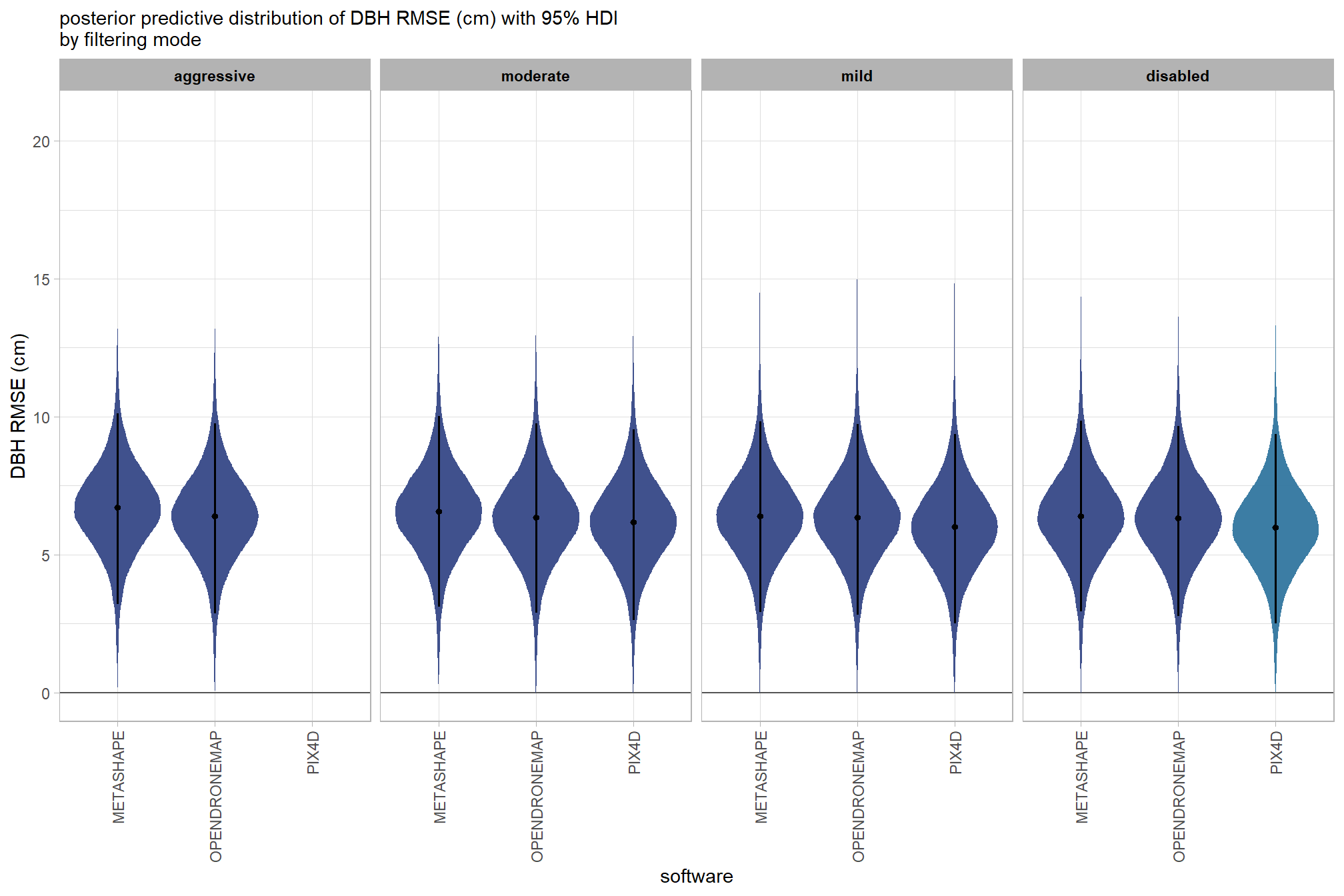
and a table of these 95% HDI values
table_temp =
  draws_temp %>%
    tidybayes::median_hdi(value) %>%
    dplyr::select(-c(.point,.interval, .width,.row)) %>%
    dplyr::arrange(software,depth_maps_generation_filtering_mode)

table_temp %>%
  dplyr::select(-c(software)) %>%
  kableExtra::kbl(
    digits = 2
    , caption = "DBH RMSE (cm)<br>95% HDI of the posterior predictive distribution"
    , col.names = c(
      "filtering mode"
      , "DBH RMSE (cm)<br>median"
      , "HDI low", "HDI high"
    )
    , escape = F
  ) %>%
  kableExtra::kable_styling() %>%
  kableExtra::pack_rows(index = table(forcats::fct_inorder(table_temp$software))) %>%
kableExtra::scroll_box(height = "8in")| filtering mode |
DBH RMSE (cm) median |
HDI low | HDI high |
|---|---|---|---|
| METASHAPE | |||
| aggressive | 6.70 | 3.12 | 10.10 |
| moderate | 6.55 | 3.02 | 10.01 |
| mild | 6.39 | 2.85 | 9.84 |
| disabled | 6.39 | 2.90 | 9.88 |
| OPENDRONEMAP | |||
| aggressive | 6.40 | 2.86 | 9.83 |
| moderate | 6.34 | 2.79 | 9.74 |
| mild | 6.34 | 2.82 | 9.82 |
| disabled | 6.31 | 2.77 | 9.76 |
| PIX4D | |||
| aggressive | 6.19 | 2.68 | 9.71 |
| moderate | 6.17 | 2.61 | 9.61 |
| mild | 6.01 | 2.45 | 9.45 |
| disabled | 5.98 | 2.42 | 9.43 |
we can also make pairwise comparisons
# calculate contrast
brms_contrast_temp = draws_temp %>%
  tidybayes::compare_levels(
    value
    , by = depth_maps_generation_filtering_mode
    , comparison = "pairwise"
  ) %>%
  dplyr::rename(contrast = depth_maps_generation_filtering_mode)

# separate contrast
brms_contrast_temp = brms_contrast_temp %>%
  dplyr::ungroup() %>%
  tidyr::separate_wider_delim(
    cols = contrast
    , delim = " - "
    , names = paste0(
      "sorter"
      , 1:(max(stringr::str_count(brms_contrast_temp$contrast, "-"))+1)
    )
    , too_few = "align_start"
    , cols_remove = F
  ) %>%
  dplyr::filter(sorter1!=sorter2) %>%
  dplyr::mutate(
    dplyr::across(
      tidyselect::starts_with("sorter")
      , .fns = function(x){factor(
        x, ordered = T
        , levels = levels(ptcld_validation_data$depth_maps_generation_filtering_mode)
      )}
    )
    , contrast = contrast %>%
      forcats::fct_reorder(
        paste0(as.numeric(sorter1), as.numeric(sorter2)) %>%
          as.numeric()
      ) %>%
      # re order for filtering mode
      forcats::fct_rev()
  ) %>%
  # median_hdi summary for coloring
  dplyr::group_by(contrast, software) %>%
  make_contrast_vars()

# remove out-of-sample obs
brms_contrast_temp = brms_contrast_temp %>%
  dplyr::inner_join(
    ptcld_validation_data %>% dplyr::distinct(software, depth_maps_generation_filtering_mode)
    , by = dplyr::join_by(software, sorter1 == depth_maps_generation_filtering_mode)
  ) %>%
  dplyr::inner_join(
    ptcld_validation_data %>% dplyr::distinct(software, depth_maps_generation_filtering_mode)
    , by = dplyr::join_by(software, sorter2 == depth_maps_generation_filtering_mode)
  )
plot it
plt_contrast(
  brms_contrast_temp
  # , caption_text = form_temp
  , y_axis_title = "filtering mode"
  , facet = "software"
  , label_size = 1.8
  , x_expand = c(0.33,0.1)
) +
  labs(
    subtitle = "posterior predictive distribution of group constrasts with 95% & 50% HDI\nby software"
    , x = "constrast DBH RMSE (cm)"
  )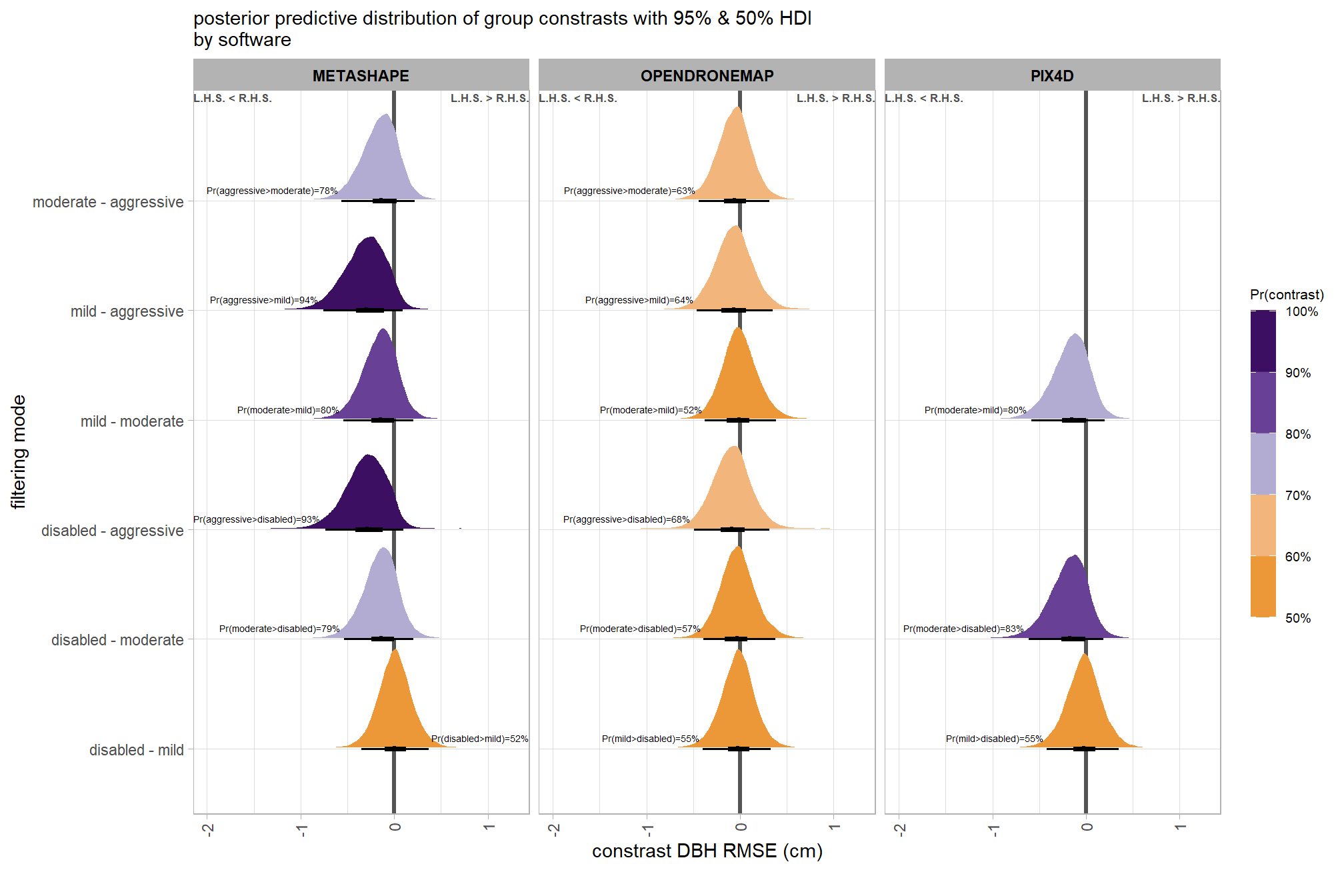
ggplot2::ggsave(
  "../data/fltr_sftwr_comp_dbh_rmse.png"
  , plot = ggplot2::last_plot() + labs(subtitle = "")
  , height = 7, width = 10.5
)
create plot for combining with other RMSE contrasts for publication
ptchwrk_fltr_sftwr_comp_dbh_rmse =
  plt_contrast(
    brms_contrast_temp
    , y_axis_title = "filtering mode contrast"
    , facet = "software"
    , label_size = 1.7
    , label = "pr_diff_lab_sm"
    , annotate_size = 1.8
  ) +
    labs(
      subtitle = "" # "constrast Height RMSE (m)"
      , x = "DBH RMSE (cm) constrast"
    ) +
    theme(
      legend.position="none"
      , axis.title.y = element_text(size = 10, face = "bold")
      , axis.title.x = element_text(size = 8)
    )
# ptchwrk_fltr_sftwr_comp_dbh_rmse
and summarize these contrasts
table_temp = brms_contrast_temp %>%
  dplyr::group_by(contrast, software, pr_lt_zero) %>%
  tidybayes::median_hdi(value) %>%
  dplyr::arrange(contrast, software) %>%
  dplyr::select(contrast, software, value, .lower, .upper, pr_lt_zero) %>%
  dplyr::arrange(software, contrast)

table_temp %>%
  dplyr::select(-c(software)) %>%
  kableExtra::kbl(
    digits = 1
    , caption = "DBH RMSE (cm)<br>95% HDI of the posterior predictive distribution of group contrasts"
    , col.names = c(
      "filtering contrast"
      , "median difference<br>DBH RMSE (cm)"
      , "HDI low", "HDI high"
      , "Pr(diff<0)"
    )
    , escape = F
  ) %>%
  kableExtra::kable_styling() %>%
  kableExtra::pack_rows(index = table(forcats::fct_inorder(table_temp$software))) %>%
kableExtra::scroll_box(height = "8in")| filtering contrast |
median difference DBH RMSE (cm) |
HDI low | HDI high | Pr(diff<0) |
|---|---|---|---|---|
| METASHAPE | ||||
| disabled - mild | 0.0 | -0.4 | 0.4 | 48% |
| disabled - moderate | -0.1 | -0.5 | 0.2 | 79% |
| disabled - aggressive | -0.3 | -0.7 | 0.1 | 93% |
| mild - moderate | -0.1 | -0.5 | 0.2 | 80% |
| mild - aggressive | -0.3 | -0.8 | 0.1 | 94% |
| moderate - aggressive | -0.1 | -0.6 | 0.2 | 78% |
| OPENDRONEMAP | ||||
| disabled - mild | 0.0 | -0.4 | 0.3 | 55% |
| disabled - moderate | 0.0 | -0.4 | 0.4 | 57% |
| disabled - aggressive | -0.1 | -0.5 | 0.3 | 68% |
| mild - moderate | 0.0 | -0.4 | 0.4 | 52% |
| mild - aggressive | -0.1 | -0.5 | 0.4 | 64% |
| moderate - aggressive | -0.1 | -0.4 | 0.3 | 63% |
| PIX4D | ||||
| disabled - mild | 0.0 | -0.4 | 0.3 | 55% |
| disabled - moderate | -0.2 | -0.6 | 0.2 | 83% |
| mild - moderate | -0.1 | -0.6 | 0.2 | 80% |
7.4.3.6 Software:Quality:Filtering - interaction
# get draws
fltr_sftwr_draws_temp =
  tidyr::crossing(
    depth_maps_generation_quality = unique(ptcld_validation_data$depth_maps_generation_quality)
    , depth_maps_generation_filtering_mode = unique(ptcld_validation_data$depth_maps_generation_filtering_mode)
    , software = unique(ptcld_validation_data$software)
  ) %>%
  tidybayes::add_epred_draws(
    brms_dbh_rmse_mod, allow_new_levels = T
    # this part is crucial
    , re_formula = ~ (1 | depth_maps_generation_quality) + # main effects
    (1 | depth_maps_generation_quality) +
    (1 | depth_maps_generation_filtering_mode) +
    (1 | software) +
    # two-way interactions
    (1 | depth_maps_generation_quality:depth_maps_generation_filtering_mode) +
    (1 | depth_maps_generation_quality:software) +
    (1 | depth_maps_generation_filtering_mode:software) +
    # three-way interactions
    (1 | depth_maps_generation_quality:depth_maps_generation_filtering_mode:software)
  ) %>%
  dplyr::rename(value = .epred) %>%
  dplyr::mutate(med = tidybayes::median_hdci(value)$y)

# plot
qlty_fltr_sftwr_dbh_rmse =
  fltr_sftwr_draws_temp %>%
    dplyr::inner_join(
      ptcld_validation_data %>% dplyr::distinct(software, depth_maps_generation_quality, depth_maps_generation_filtering_mode)
      , by = dplyr::join_by(software, depth_maps_generation_quality, depth_maps_generation_filtering_mode)
    ) %>%
    dplyr::mutate(depth_maps_generation_quality = depth_maps_generation_quality %>% forcats::fct_rev()) %>%
    ggplot(
      mapping = aes(
        y = value
        , x = depth_maps_generation_filtering_mode
        , fill = med
      )
    ) +
    geom_hline(yintercept = 0, color = "gray33") +
    tidybayes::stat_eye(
      point_interval = median_hdi, .width = .95
      , slab_alpha = 0.98
      , interval_color = "black", linewidth = 1
      , point_color = "black", point_fill = "black", point_size = 1
    ) +
    scale_fill_stepsn(
      n.breaks = 5
      , colors = viridis::mako(n = 5, begin = 0.2, end = 0.9, direction = -1)
      , limits = c(0,lmt_dbh_cm_rmse)
      , labels = scales::comma_format(accuracy = 0.01)
      , show.limits = T
    ) +
    facet_grid(
      rows = vars(software)
      , cols = vars(depth_maps_generation_quality)
      # , switch = "y"
    ) +
    scale_y_continuous(limits = c(-0.02,NA)) +
    labs(
      x = "filtering mode", y = "DBH RMSE (cm)"
      , subtitle = "posterior predictive distribution of DBH RMSE (cm) with 95% HDI\nby dense cloud quality and software"
      # , caption = form_temp
    ) +
    theme_light() +
    theme(
      legend.position = "none"
      , legend.direction  = "horizontal"
      , axis.text.x = element_text(angle = 90, vjust = 0.5, hjust = 1)
      , strip.text = element_text(color = "black", face = "bold")
      , panel.grid = element_blank()
      # , strip.placement = "outside"
    ) +
    guides(
      fill = guide_legend(override.aes = list(shape = NA, size = 6, alpha = 0.9, lwd = NA))
    )
# print it
qlty_fltr_sftwr_dbh_rmse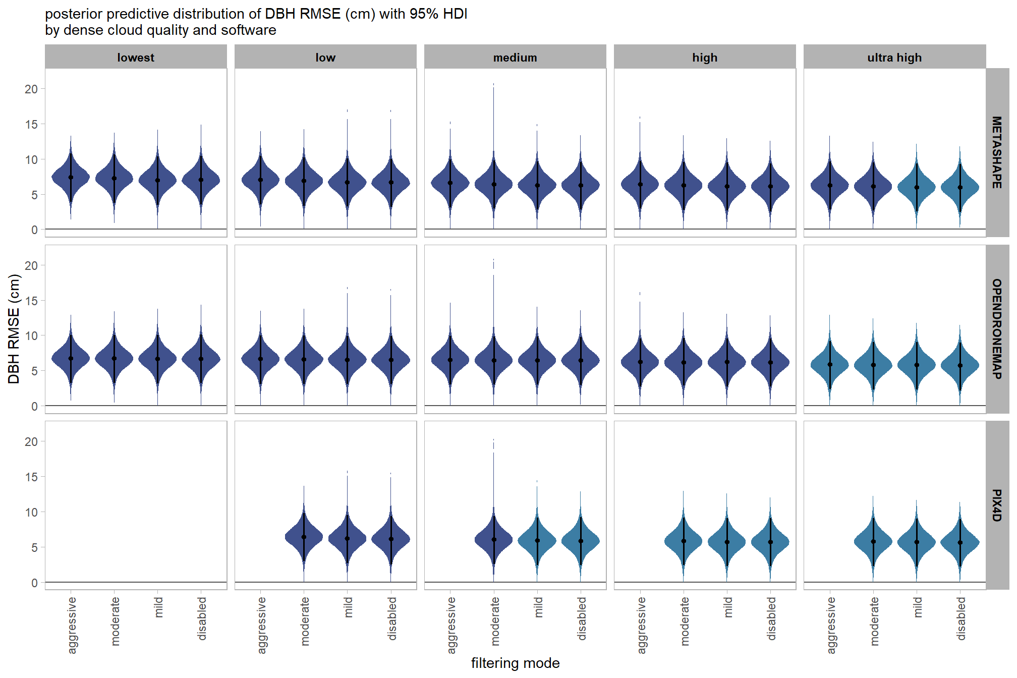
and a table of these 95% HDI values
table_temp =
  fltr_sftwr_draws_temp %>%
  tidybayes::median_hdi(value) %>%
  dplyr::inner_join(
    ptcld_validation_data %>% dplyr::distinct(software, depth_maps_generation_quality, depth_maps_generation_filtering_mode)
    , by = dplyr::join_by(software, depth_maps_generation_quality, depth_maps_generation_filtering_mode)
  ) %>%
  dplyr::mutate(depth_maps_generation_quality = depth_maps_generation_quality %>% forcats::fct_rev()) %>%
  dplyr::select(c(
    software, depth_maps_generation_quality, depth_maps_generation_filtering_mode
    , value, .lower, .upper
  )) %>%
  dplyr::ungroup() %>%
  dplyr::arrange(software, depth_maps_generation_quality, depth_maps_generation_filtering_mode)

table_temp %>%
  # dplyr::select(-c(software)) %>%
  kableExtra::kbl(
    digits = 2
    , caption = "DBH RMSE (cm)<br>95% HDI of the posterior predictive distribution"
    , col.names = c(
      "software", "quality", "filtering mode"
      , "DBH RMSE (cm)<br>median"
      , "HDI low", "HDI high"
    )
    , escape = F
  ) %>%
  kableExtra::kable_styling() %>%
  # kableExtra::pack_rows(index = table(forcats::fct_inorder(table_temp$software))) %>%
  kableExtra::collapse_rows(columns = 1:2, valign = "top") %>%
kableExtra::scroll_box(height = "8in")| software | quality | filtering mode |
DBH RMSE (cm) median |
HDI low | HDI high |
|---|---|---|---|---|---|
| METASHAPE | lowest | aggressive | 7.40 | 3.85 | 10.73 |
| moderate | 7.26 | 3.76 | 10.66 | ||
| mild | 6.99 | 3.51 | 10.43 | ||
| disabled | 7.03 | 3.55 | 10.44 | ||
| low | aggressive | 7.04 | 3.49 | 10.37 | |
| moderate | 6.87 | 3.34 | 10.25 | ||
| mild | 6.65 | 3.13 | 10.02 | ||
| disabled | 6.66 | 3.15 | 10.01 | ||
| medium | aggressive | 6.60 | 3.09 | 9.99 | |
| moderate | 6.42 | 2.92 | 9.80 | ||
| mild | 6.28 | 2.78 | 9.66 | ||
| disabled | 6.28 | 2.78 | 9.65 | ||
| high | aggressive | 6.42 | 2.91 | 9.78 | |
| moderate | 6.23 | 2.72 | 9.62 | ||
| mild | 6.11 | 2.61 | 9.52 | ||
| disabled | 6.12 | 2.61 | 9.52 | ||
| ultra high | aggressive | 6.25 | 2.72 | 9.59 | |
| moderate | 6.09 | 2.59 | 9.50 | ||
| mild | 5.99 | 2.50 | 9.39 | ||
| disabled | 5.97 | 2.46 | 9.35 | ||
| OPENDRONEMAP | lowest | aggressive | 6.76 | 3.20 | 10.08 |
| moderate | 6.71 | 3.12 | 10.02 | ||
| mild | 6.67 | 3.17 | 10.08 | ||
| disabled | 6.66 | 3.13 | 10.06 | ||
| low | aggressive | 6.65 | 3.10 | 9.99 | |
| moderate | 6.59 | 3.09 | 9.96 | ||
| mild | 6.54 | 3.01 | 9.90 | ||
| disabled | 6.51 | 3.01 | 9.89 | ||
| medium | aggressive | 6.54 | 3.01 | 9.92 | |
| moderate | 6.46 | 2.98 | 9.87 | ||
| mild | 6.47 | 2.95 | 9.86 | ||
| disabled | 6.46 | 2.96 | 9.87 | ||
| high | aggressive | 6.24 | 2.73 | 9.60 | |
| moderate | 6.16 | 2.73 | 9.62 | ||
| mild | 6.20 | 2.68 | 9.57 | ||
| disabled | 6.18 | 2.66 | 9.57 | ||
| ultra high | aggressive | 5.85 | 2.30 | 9.21 | |
| moderate | 5.78 | 2.27 | 9.15 | ||
| mild | 5.82 | 2.27 | 9.15 | ||
| disabled | 5.76 | 2.21 | 9.10 | ||
| PIX4D | low | moderate | 6.46 | 2.96 | 9.87 |
| mild | 6.20 | 2.62 | 9.52 | ||
| disabled | 6.15 | 2.64 | 9.57 | ||
| medium | moderate | 6.06 | 2.59 | 9.46 | |
| mild | 5.90 | 2.42 | 9.30 | ||
| disabled | 5.88 | 2.38 | 9.28 | ||
| high | moderate | 5.84 | 2.30 | 9.19 | |
| mild | 5.72 | 2.31 | 9.21 | ||
| disabled | 5.71 | 2.34 | 9.24 | ||
| ultra high | moderate | 5.79 | 2.22 | 9.13 | |
| mild | 5.68 | 2.09 | 9.01 | ||
| disabled | 5.63 | 2.05 | 8.97 |
we can also make pairwise comparisons
# calculate contrast
brms_contrast_temp = fltr_sftwr_draws_temp %>%
  tidybayes::compare_levels(
    value
    , by = depth_maps_generation_filtering_mode
    , comparison = "pairwise"
  ) %>%
  dplyr::rename(contrast = depth_maps_generation_filtering_mode)

# separate contrast
brms_contrast_temp = brms_contrast_temp %>%
  dplyr::ungroup() %>%
  tidyr::separate_wider_delim(
    cols = contrast
    , delim = " - "
    , names = paste0(
      "sorter"
      , 1:(max(stringr::str_count(brms_contrast_temp$contrast, "-"))+1)
    )
    , too_few = "align_start"
    , cols_remove = F
  ) %>%
  dplyr::filter(sorter1!=sorter2) %>%
  dplyr::mutate(
    dplyr::across(
      tidyselect::starts_with("sorter")
      , .fns = function(x){factor(
        x, ordered = T
        , levels = levels(ptcld_validation_data$depth_maps_generation_filtering_mode)
      )}
    )
    , contrast = contrast %>%
      forcats::fct_reorder(
        paste0(as.numeric(sorter1), as.numeric(sorter2)) %>%
          as.numeric()
      ) %>%
      # re order for filtering mode
      forcats::fct_rev()
  ) %>%
  # median_hdi summary for coloring
  dplyr::group_by(contrast, software, depth_maps_generation_quality) %>%
  make_contrast_vars()

# remove out-of-sample obs
brms_contrast_temp = brms_contrast_temp %>%
  dplyr::inner_join(
    ptcld_validation_data %>% dplyr::distinct(software, depth_maps_generation_quality, depth_maps_generation_filtering_mode)
    , by = dplyr::join_by(software, depth_maps_generation_quality, sorter1==depth_maps_generation_filtering_mode)
  ) %>%
  dplyr::inner_join(
    ptcld_validation_data %>% dplyr::distinct(software, depth_maps_generation_quality, depth_maps_generation_filtering_mode)
    , by = dplyr::join_by(software, depth_maps_generation_quality, sorter2==depth_maps_generation_filtering_mode)
  ) %>%
  dplyr::mutate(depth_maps_generation_quality = depth_maps_generation_quality %>% forcats::fct_rev())
plot it
brms_contrast_temp %>%
  plt_contrast(
    facet = c("depth_maps_generation_quality", "software")
    , y_axis_title = "filtering mode"
    , label_size = 0
    , x_expand = c(-0.1,-0.1)
  ) +
  facet_grid(
    rows = vars(software)
    , cols = vars(depth_maps_generation_quality)
  ) +
  labs(
    subtitle = "posterior predictive distribution of group constrasts with 95% & 50% HDI\nby dense cloud quality and software"
    , x = "constrast DBH RMSE (cm)"
  )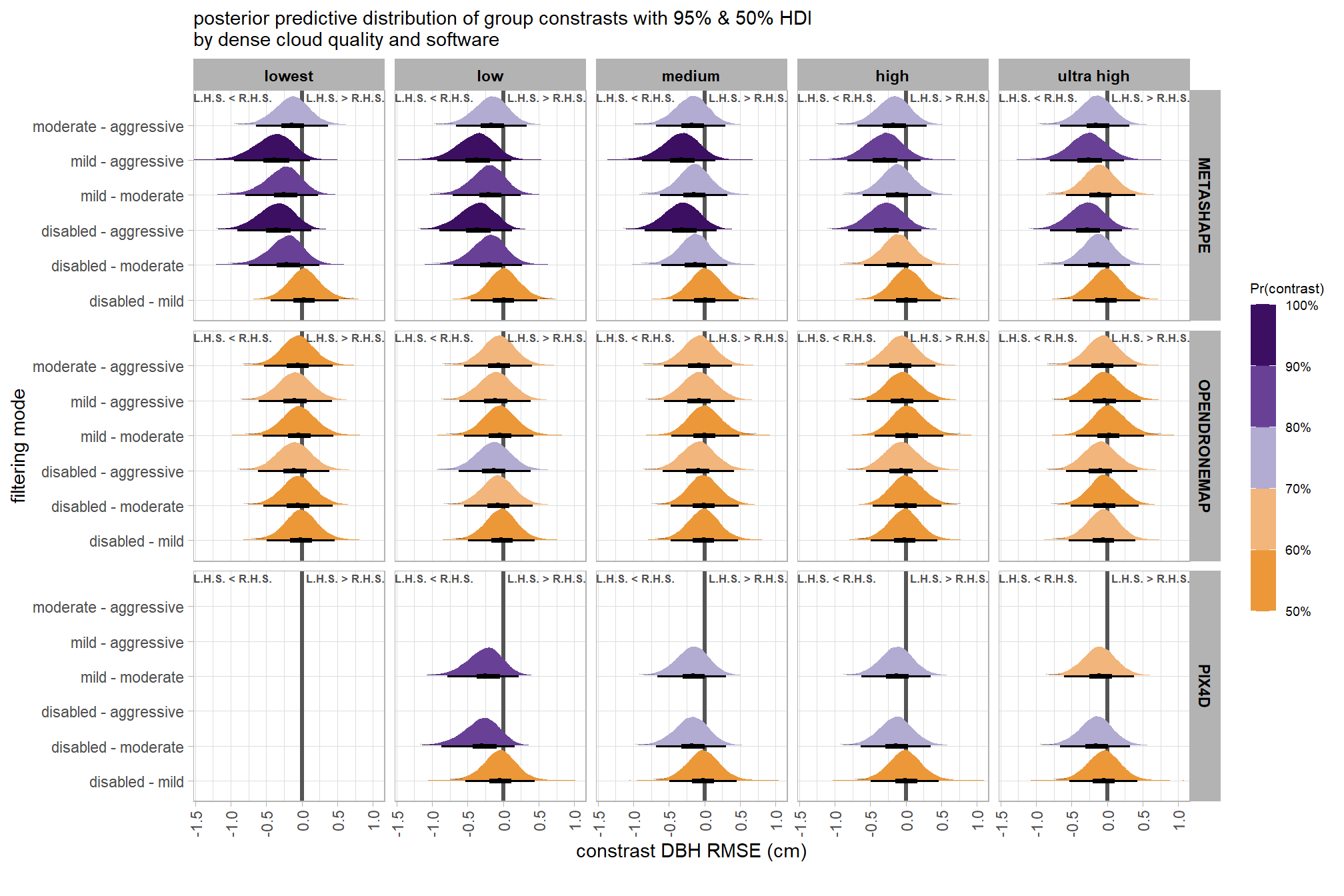
ggplot2::ggsave(
  "../data/qlty_fltr_sftwr_comp_dbh_rmse.png"
  , plot = ggplot2::last_plot() + labs(subtitle = "")
  , height = 7, width = 10.5
)
Export some final images for publication
p1_temp = qlty_fltr_sftwr_dbh_me + labs(subtitle = "A: DBH Mean Error (cm)") + theme(plot.subtitle = element_text(face="bold"))
p2_temp = qlty_fltr_sftwr_dbh_rmse + labs(subtitle = "B: DBH RMSE (cm)") + theme(plot.subtitle = element_text(face="bold"))
# export
p1_temp / p2_temp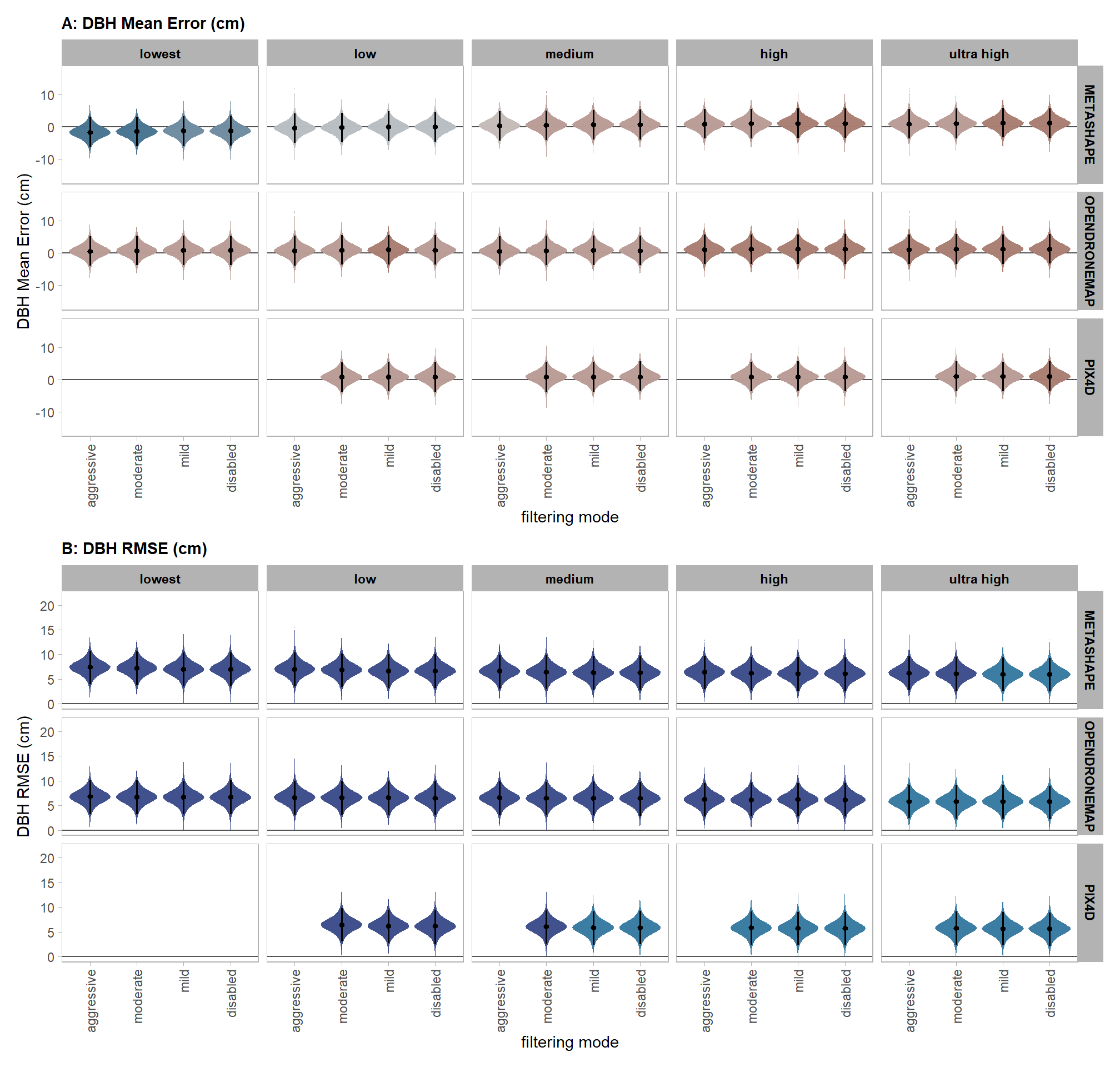
ggplot2::ggsave(
    filename = paste0("../data/qlty_fltr_sftwr_dbh_comb.jpeg")
    , plot = ggplot2::last_plot()
    , width = 8.5
    , height = 11
    , units = "in"
    , dpi = "print"
  )
patchwork of Height RMSE contrasts
layout_temp = c(
    # area(t, l, b, r)
    patchwork::area(2, 1, 2, 1)
    , patchwork::area(2, 3, 2, 3)
    , patchwork::area(4, 1, 4, 3)
  )
  # check the layout
  # plot(layout_temp)
############################
# patchwork for height
############################
  ptchwrk_qlty_sftwr_comp_ht_rmse +
    labs(subtitle = "A: Quality Contrast by Software") +
    theme(plot.background = element_rect(colour = "gray88", fill=NA, size=3)) +
  ptchwrk_fltr_sftwr_comp_ht_rmse +
    labs(subtitle = "B: Filtering Mode Contrast by Software") +
    theme(plot.background = element_rect(colour = "gray88", fill=NA, size=3)) +
  patchwork::free(
    ptchwrk_sftwr_qlty_comp_ht_rmse +
    labs(subtitle = "C: Software Contrast by Quality") +
    theme(plot.background = element_rect(colour = "gray88", fill=NA, size=3)) ) +
  # plot_annotation(tag_levels = list(c('#', '&'), '1')) +
  patchwork::plot_layout(
    design = layout_temp
    , widths = c(1,0.01,1)
    , heights = c(0.01,1,0.01,1,0.01)
  ) &
  scale_x_continuous(
    limits = c(-0.7,0.45)
    , breaks = seq(-0.8,0.4,0.2)
    , labels = seq(-0.8,0.4,0.2) %>% scales::number(accuracy = 0.1)
  ) &
  theme(
    axis.title.y = element_blank()
    , plot.subtitle = element_text(face = "bold", hjust = 0.0)
    # , plot.background = element_rect(colour = "gray88", fill=NA, size=3)
  )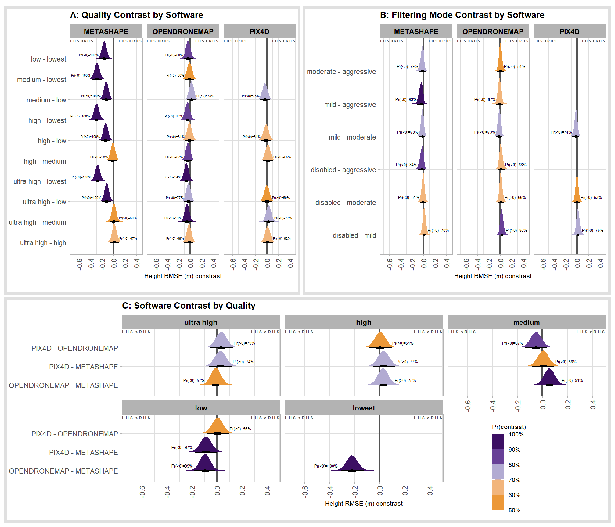
ggplot2::ggsave(
    filename = paste0("../data/all_ht_rmse_contrasts.jpeg")
    , plot = ggplot2::last_plot()
    , width = 11
    , height = 8.5
    , units = "in"
    , dpi = "print"
  )
patchwork of DBH RMSE contrasts
layout_temp = c(
    # area(t, l, b, r)
    patchwork::area(2, 1, 2, 1)
    , patchwork::area(2, 3, 2, 3)
    , patchwork::area(4, 1, 4, 3)
  )
  # check the layout
  # plot(layout_temp)
############################
# patchwork for height
############################
  ptchwrk_qlty_sftwr_comp_dbh_rmse +
    labs(subtitle = "A: Quality Contrast by Software") +
    theme(plot.background = element_rect(colour = "gray88", fill=NA, size=3)) +
  ptchwrk_fltr_sftwr_comp_dbh_rmse +
    labs(subtitle = "B: Filtering Mode Contrast by Software") +
    theme(plot.background = element_rect(colour = "gray88", fill=NA, size=3)) +
  patchwork::free(
    ptchwrk_sftwr_qlty_comp_dbh_rmse +
    labs(subtitle = "C: Software Contrast by Quality") +
    theme(plot.background = element_rect(colour = "gray88", fill=NA, size=3)) ) +
  # plot_annotation(tag_levels = list(c('#', '&'), '1')) +
  patchwork::plot_layout(
    design = layout_temp
    , widths = c(1,0.01,1)
    , heights = c(0.01,1,0.01,1,0.01)
  ) &
  scale_x_continuous(
    limits = c(-3,2)
    , breaks = seq(-4,2,2)
    , labels = seq(-4,2,2) %>% scales::number(accuracy = 1)
  ) &
  theme(
    axis.title.y = element_blank()
    , plot.subtitle = element_text(face = "bold", hjust = 0.0)
    # , plot.background = element_rect(colour = "gray88", fill=NA, size=3)
  )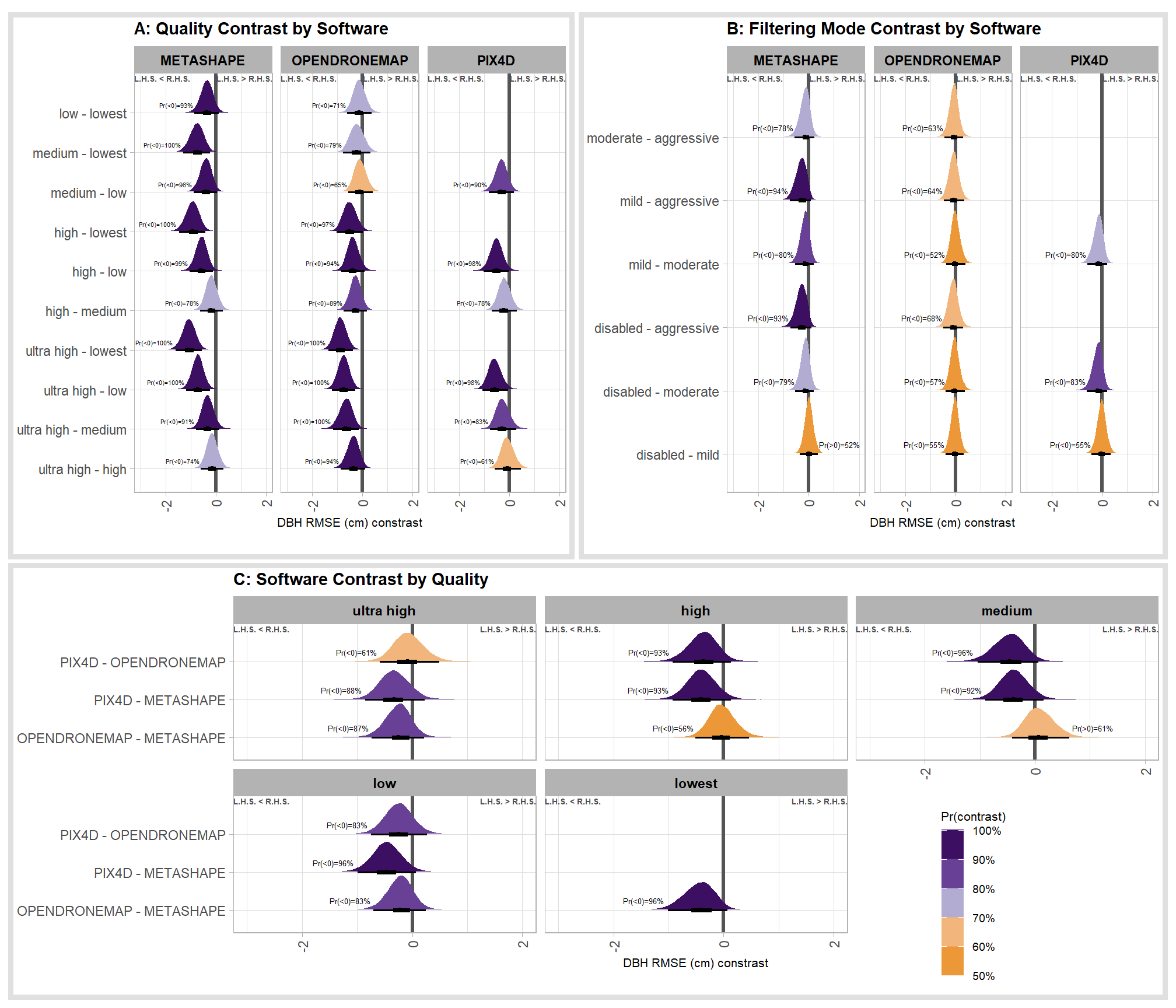
7.5 Posterior Predictive Checks
Markov chain Monte Carlo (MCMC) simulations were conducted using the brms package (Bürkner 2017) to estimate posterior predictive distributions of the parameters of interest. We ran three chains of 100,000 iterations with the first 50,000 discarded as burn-in. Trace-plots were utilized to visually assess model convergence and sufficient convergence was checked with \(\hat{R}\) values near 1 (Brooks & Gelman, 1998). Posterior predictive checks were used to evaluate model goodness-of-fit by comparing data simulated from the model with the observed data used to estimate the model parameters (Hobbs & Hooten, 2015). Calculating the proportion of MCMC iterations in which the test statistic (i.e., mean and sum of squares) from the simulated data and observed data are more extreme than one another provides the Bayesian P-value. Lack of fit is indicated by a value close to 0 or 1 while a value of 0.5 indicates perfect fit (Hobbs & Hooten, 2015).
To learn more about this approach to posterior predictive checks, check out Gabry’s (2022) vignette, Graphical posterior predictive checks using the bayesplot package.
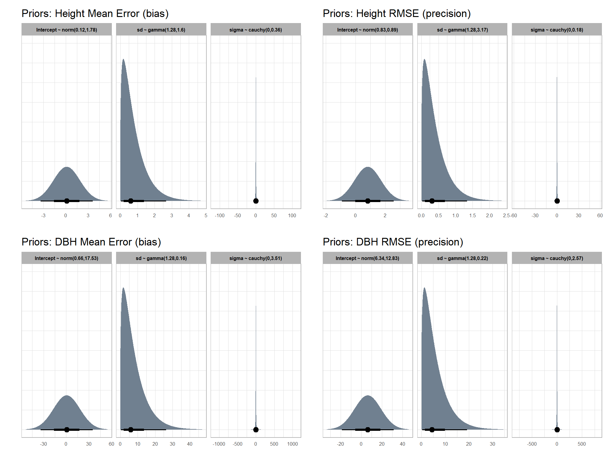
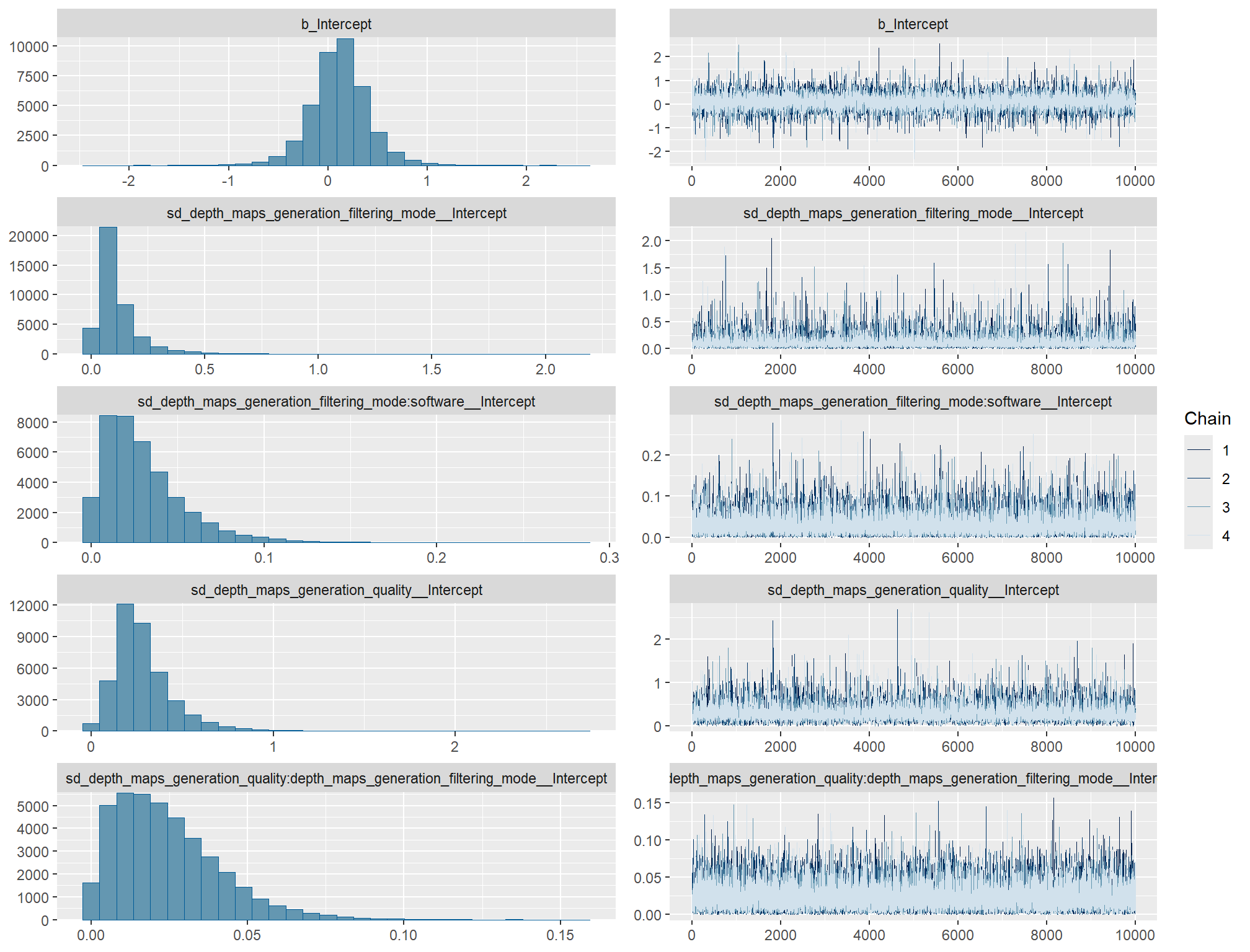
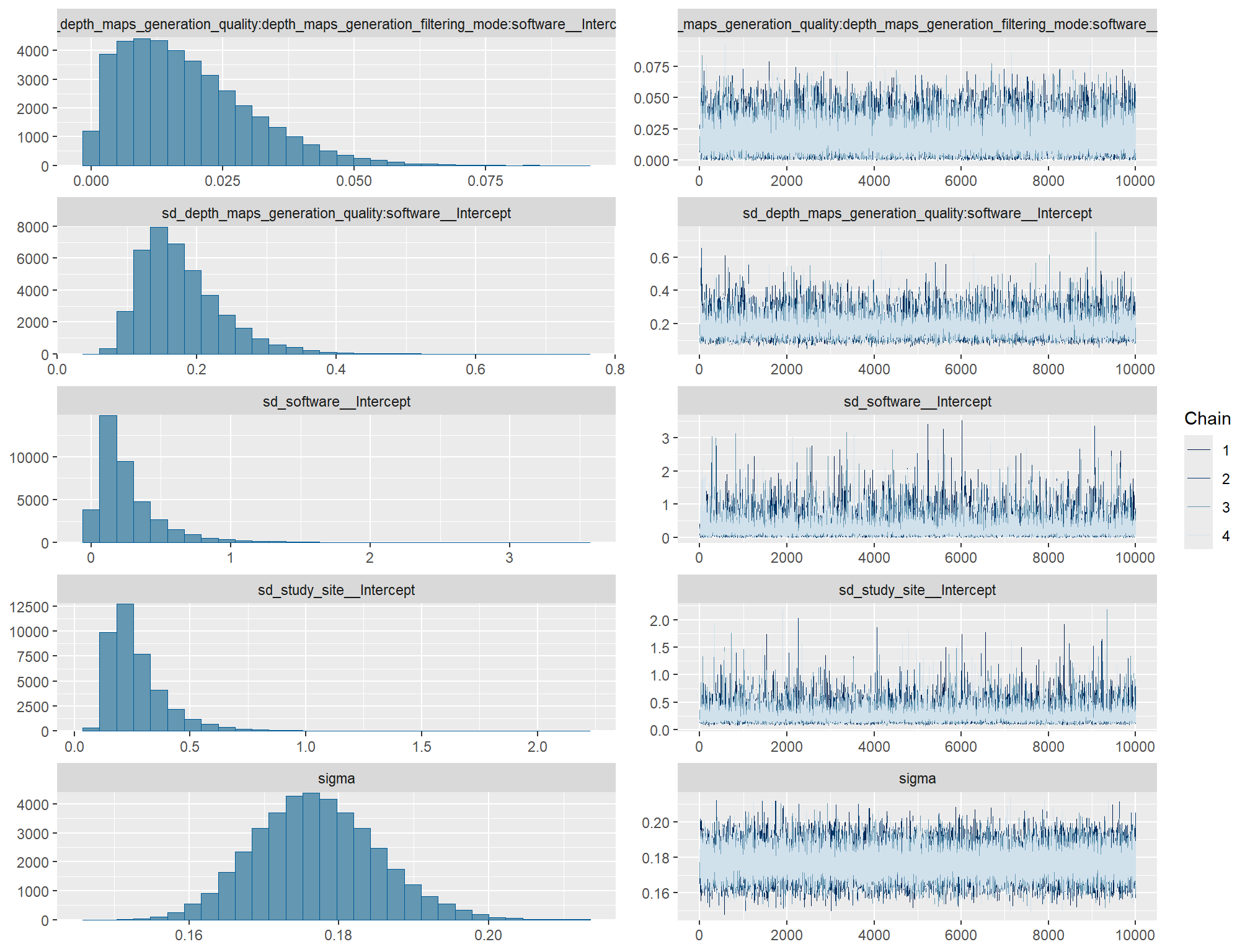
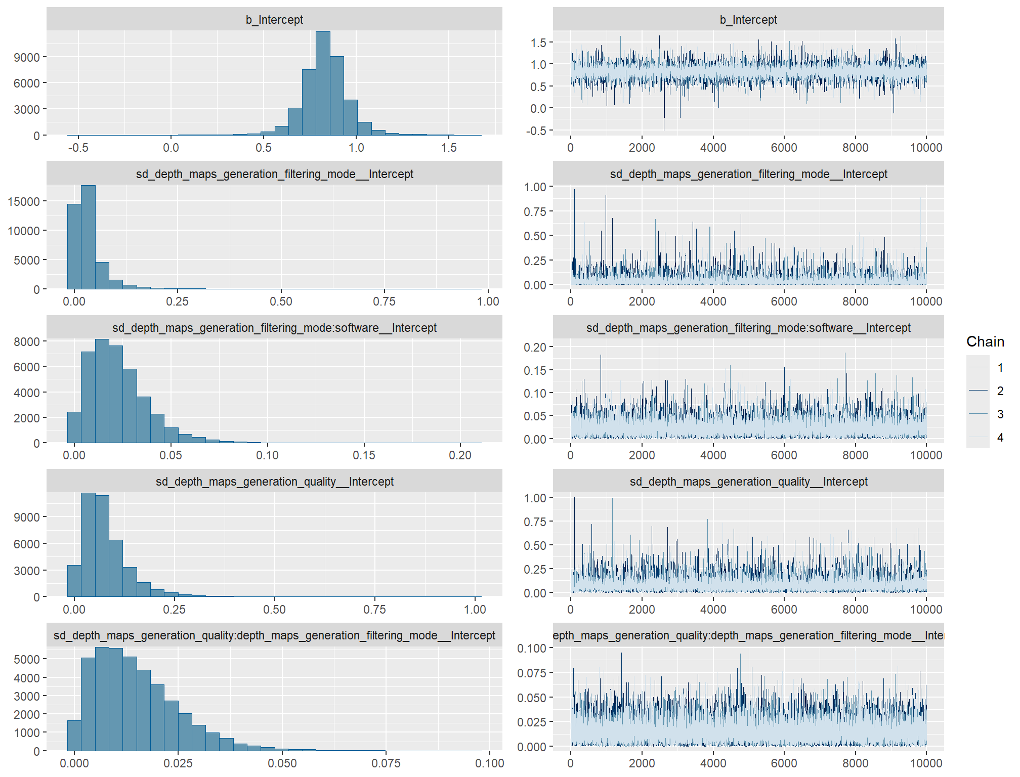
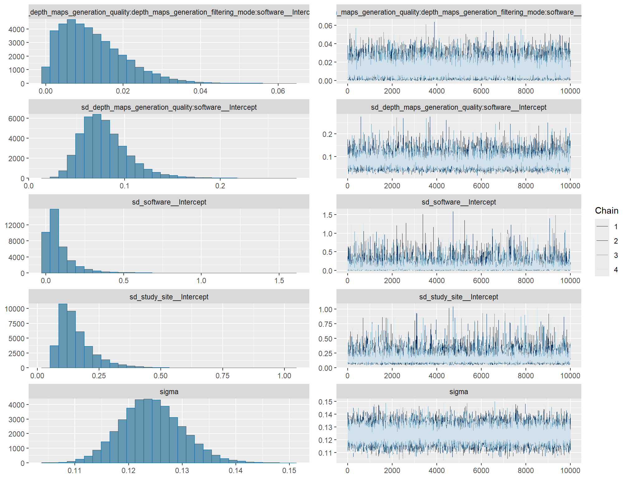
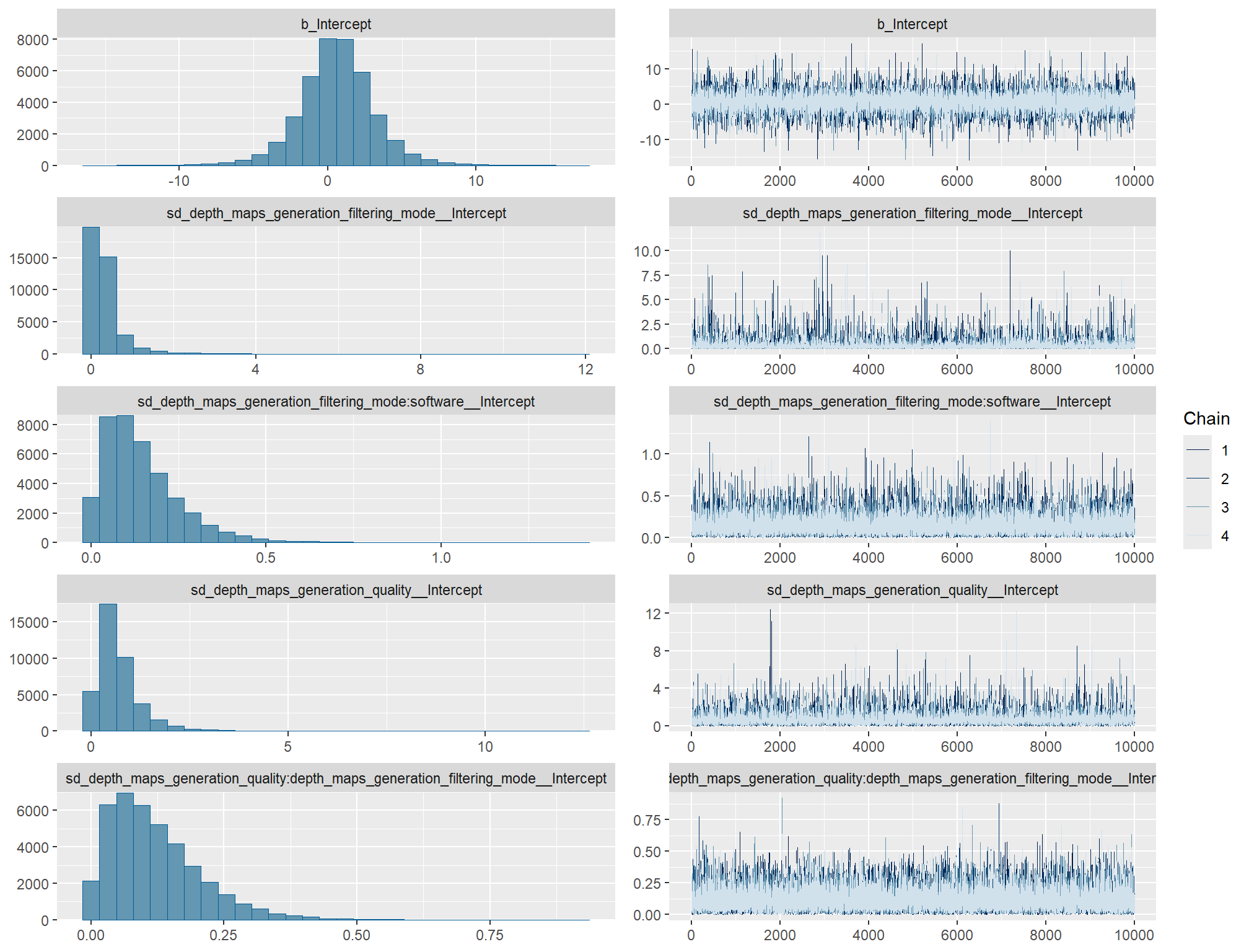
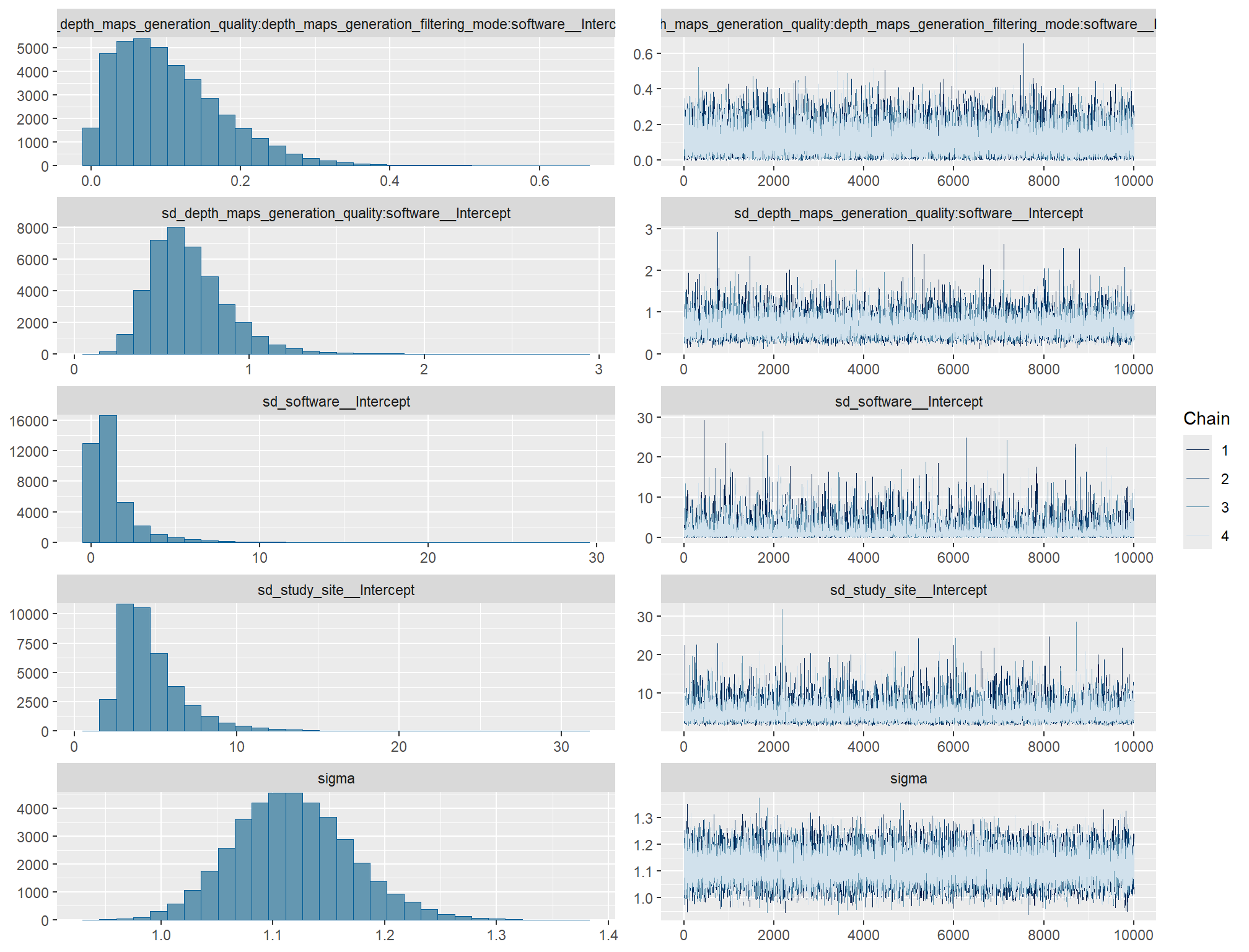
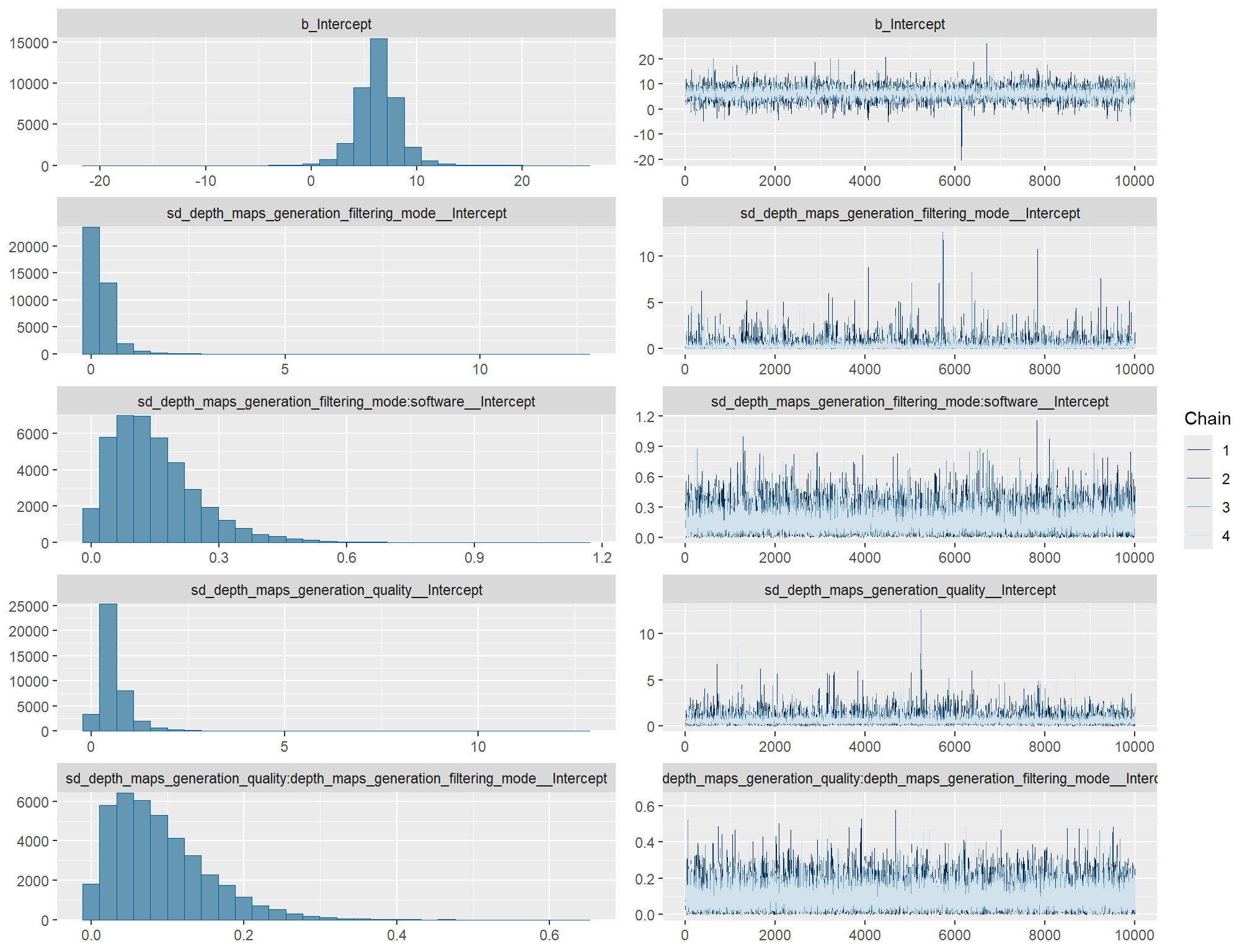
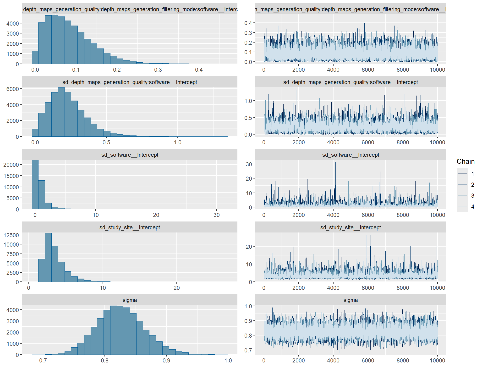
7.5.3 \(\hat{R}\) values
plt_rhat_temp <- function(my_mod) {
  my_mod %>%
    brms::rhat() %>%
    as.data.frame() %>%
    tibble::rownames_to_column(var = "parameter") %>%
    dplyr::rename_with(tolower) %>%
    dplyr::rename(rhat = 2) %>%
    dplyr::filter(
      stringr::str_starts(parameter, "b_")
      | stringr::str_starts(parameter, "r_")
      | stringr::str_starts(parameter, "sd_")
      | parameter == "phi"
      | parameter == "sigma"
    ) %>%
    dplyr::mutate(
      parameter = parameter %>%
        stringr::str_replace_all("depth_maps_generation_quality", "quality") %>%
        stringr::str_replace_all("depth_maps_generation_filtering_mode", "filtering")
      , chk = (rhat <= 1*0.998 | rhat >= 1*1.002)
    ) %>%
    ggplot(aes(x = rhat, y = parameter, color = chk, fill = chk)) +
    geom_vline(xintercept = 1, linetype = "dashed", color = "gray44", lwd = 1.2) +
    geom_vline(xintercept = 1*0.998, lwd = 1.5) +
    geom_vline(xintercept = 1*1.002, lwd = 1.5) +
    geom_vline(xintercept = 1*0.999, lwd = 1.2, color = "gray33") +
    geom_vline(xintercept = 1*1.001, lwd = 1.2, color = "gray33") +
    geom_point() +
    scale_fill_manual(values = c("navy", "firebrick")) +
    scale_color_manual(values = c("navy", "firebrick")) +
    scale_y_discrete(NULL, breaks = NULL) +
    labs(
      x = latex2exp::TeX("$\\hat{R}$")
      , subtitle = latex2exp::TeX("MCMC chain convergence check for $\\hat{R}$ values")
    ) +
    theme_light() +
    theme(
      legend.position = "none"
      , axis.text.y = element_text(size = 3)
      , panel.grid.major.x = element_blank()
      , panel.grid.minor.x = element_blank()
      , plot.title = element_text(size = 9)
      , plot.subtitle = element_text(size = 8)
      , axis.title.y = element_blank()
      , axis.title.x = element_text(size = 9)
      , panel.grid = element_blank()
      , axis.text.x = element_text(size = 6.5)
    )
}
# plot together with patchwork
# height mean error
brms_ht_me_mod %>% plt_rhat_temp() + labs(title = "Height Mean Error (bias)") +
# height rmse
brms_ht_rmse_mod %>% plt_rhat_temp() + labs(title = "Height RMSE (precision)") +
# dbh me
brms_dbh_me_mod %>% plt_rhat_temp() + labs(title = "DBH Mean Error (bias)") +
# dbh rmse
brms_dbh_rmse_mod %>% plt_rhat_temp() + labs(title = "DBH RMSE (precision)") &
  theme(plot.subtitle = element_blank())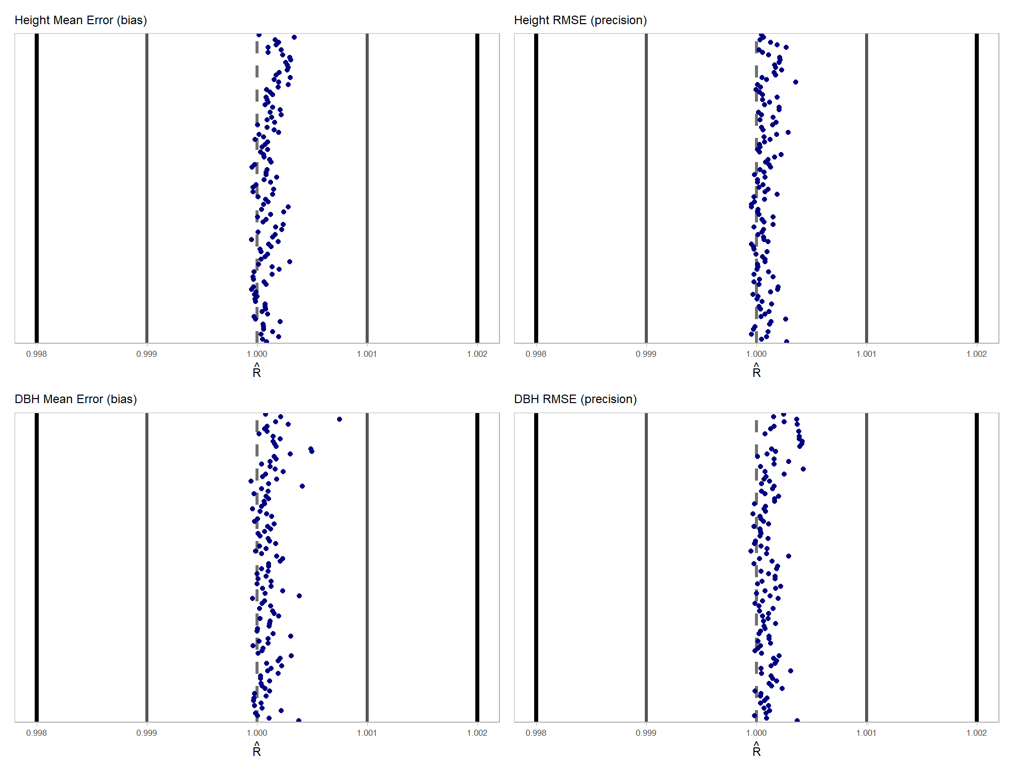
7.5.4 ESS values
The effective length of an MCMC chain is indicated by the effective sample size (ESS), which refers to the sample size of the MCMC chain not to the sample size of the data Kruschke (2015) notes:
One simple guideline is this: For reasonably accurate and stable estimates of the limits of the 95% HDI, an ESS of 10,000 is recommended. This is merely a heuristic based on experience with practical applications, it is not a requirement. If accuracy of the HDI limits is not crucial for your application, then a smaller ESS may be sufficient. (p.184)
plt_ess_temp <- function(my_mod) {
# get ess values from model summary
dplyr::bind_rows(
    summary(my_mod) %>%
      purrr::pluck("random") %>%
      purrr::flatten() %>%
      purrr::keep_at(~ .x == "Bulk_ESS") %>%
      unlist() %>%
      dplyr::as_tibble()
    , summary(my_mod) %>%
      purrr::pluck("fixed") %>%
      purrr::flatten() %>%
      purrr::keep_at(~ .x == "Bulk_ESS") %>%
      unlist() %>%
      dplyr::as_tibble()
  ) %>%
  dplyr::rename(ess = 1) %>%
  dplyr::mutate(parameter = dplyr::row_number(), chk = ess<10000) %>%
  ggplot(aes(x = ess, y = parameter, color = chk, fill = chk)) +
  geom_vline(xintercept = 10000, linetype = "dashed", color = "gray44", lwd = 1.2) +
  geom_segment( aes(x = 0, xend=ess, yend=parameter), color="black") +
  geom_point() +
  scale_fill_manual(values = c("blue4", "blue3")) +
  scale_color_manual(values = c("blue4", "blue3")) +
  scale_y_continuous(NULL, breaks = NULL) +
  scale_x_continuous(labels = scales::comma) +
  labs(
    x = "ESS"
    , subtitle = "MCMC chain resolution check for effective sample size (ESS) values"
    , y = ""
  ) +
  theme_light() +
  theme(
    legend.position = "none"
    , axis.text.y = element_text(size = 4)
    , panel.grid.major.x = element_blank()
    , panel.grid.minor.x = element_blank()
    , plot.title = element_text(size = 9)
    , plot.subtitle = element_text(size = 8)
    , axis.title.y = element_blank()
    , axis.title.x = element_text(size = 9)
    , axis.text.x = element_text(size = 6.5)
  )
}

# plot together with patchwork
# height mean error
brms_ht_me_mod %>% plt_ess_temp() + labs(title = "Height Mean Error (bias)") +
# height rmse
brms_ht_rmse_mod %>% plt_ess_temp() + labs(title = "Height RMSE (precision)") +
# dbh me
brms_dbh_me_mod %>% plt_ess_temp() + labs(title = "DBH Mean Error (bias)") +
# dbh rmse
brms_dbh_rmse_mod %>% plt_ess_temp() + labs(title = "DBH RMSE (precision)") &
  theme(plot.subtitle = element_blank())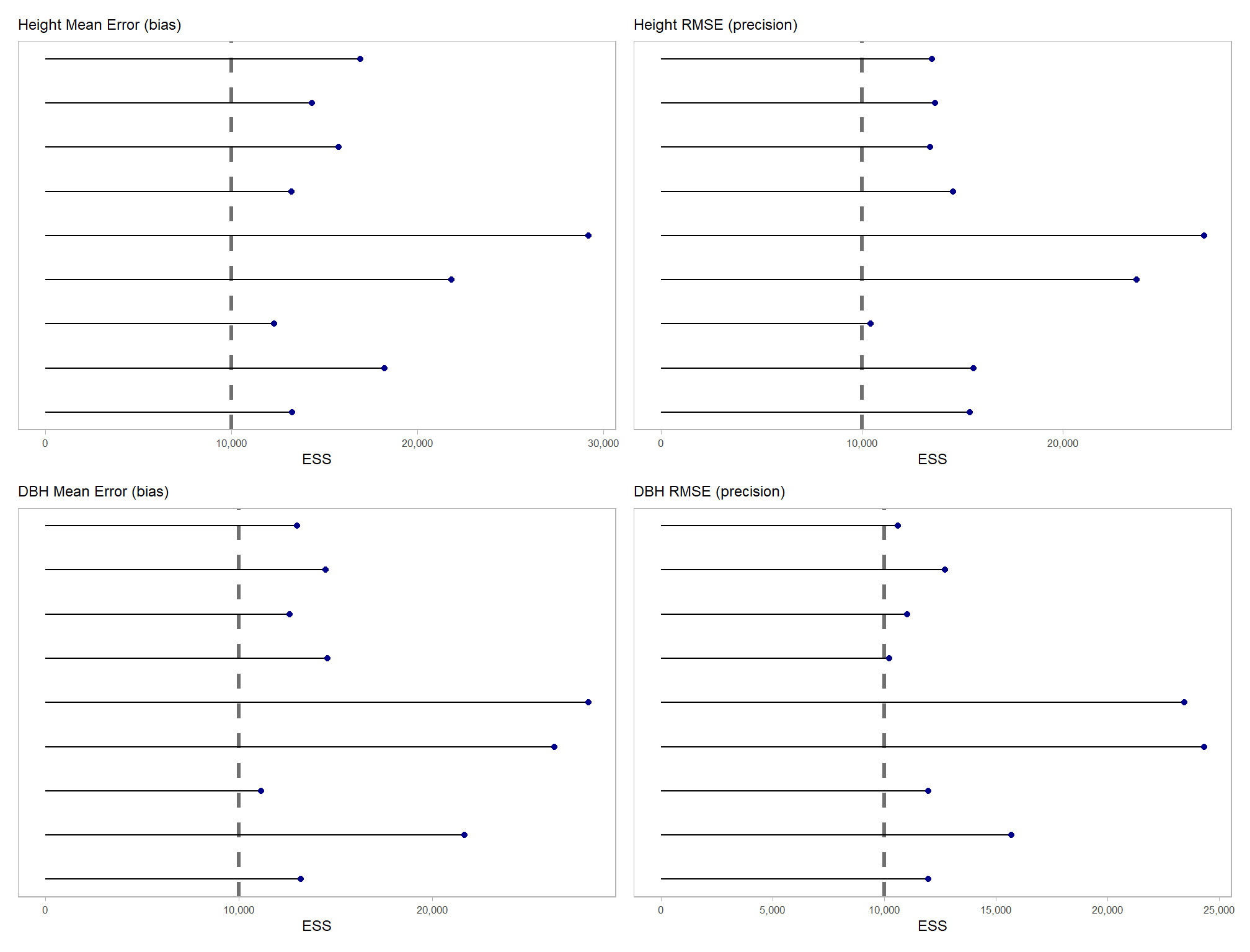
7.5.5 Mean and SD
posterior predictive check for the overall model combining mean and sd
plt_pp_temp <- function(my_mod) {
  my_mod %>%
  brms::pp_check(type = "stat_2d", ndraws = 5000) +
    theme_light() +
    theme(
      legend.position = "top", legend.direction = "horizontal"
      , legend.text = element_text(size = 8)
      , plot.title = element_text(size = 9)
    )
}
# plot together with patchwork
# height mean error
brms_ht_me_mod %>% plt_pp_temp() + labs(title = "Height Mean Error (bias)") +
# height rmse
brms_ht_rmse_mod %>% plt_pp_temp() + labs(title = "Height RMSE (precision)") +
# dbh me
brms_dbh_me_mod %>% plt_pp_temp() + labs(title = "DBH Mean Error (bias)") +
# dbh rmse
brms_dbh_rmse_mod %>% plt_pp_temp() + labs(title = "DBH RMSE (precision)")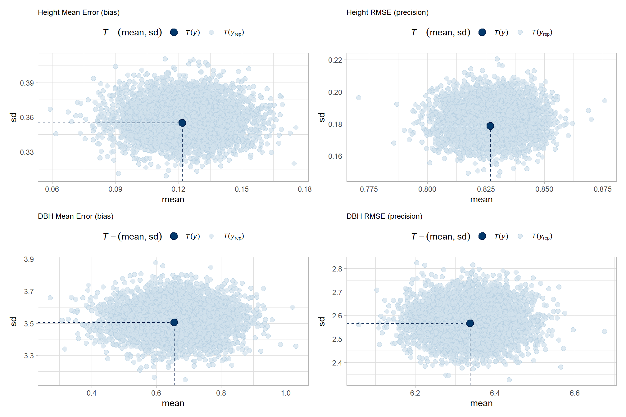
7.5.5.1 Bayesian p-value
The Bayesian p-value is the probability that a test statistic in the reference distribution exceeds its value in the data. The Bayesian p-value is calculated from the posterior predictive distribution of the new data and the distribution of the observed data. We estimate the probability that the test statistic calculated from “new” data arising from our model (\(y_{new}\)) is more extreme than the test statistic calculated from the observed data (\(y\)): \(\text{P-value}(y) = Pr(T(y_{new}) > T(y))\) where the test statistic \(T(y)\) describes the distribution of the data as a summary of the data; it could be the mean, variance, the coefficient of variation, the kurtosis, the maximum, or the minimum of the observed data set, or it might be an “omnibus” statistic like a squared discrepancy or a chi-square value Hobbs and Hooten (2015, p. 188)
Bayesian P values for mean and standard deviation test statistics The P values for the mean (P mean) give the probability that the mean of the data of new, out-of-sample observations simulated from the model exceeds the mean of the observed data. The P values for the standard deviation (P SD) give the probability that the standard deviation of new, out-of-sample observations simulated from the model exceeds the standard deviation of the observed data. Large (\(\gtrapprox 0.90\)) or small (\(\lessapprox 0.10\)) values indicate lack of fit. Hobbs and Hooten (2015);Hobbs et al. (2024, Appendix S2 p. 8)
Check the Bayesian p-values between the models
# get the model p-values
set.seed(16) # replicate results
dplyr::bind_rows(
    get_mod_p_val(brms_ht_me_mod, ndraws = 5000) %>%
      dplyr::mutate(model = "brms_ht_me_mod")
    , get_mod_p_val(brms_ht_rmse_mod, ndraws = 5000) %>%
      dplyr::mutate(model = "brms_ht_rmse_mod")
    , get_mod_p_val(brms_dbh_me_mod, ndraws = 5000) %>%
      dplyr::mutate(model = "brms_dbh_me_mod")
    , get_mod_p_val(brms_dbh_rmse_mod, ndraws = 5000) %>%
      dplyr::mutate(model = "brms_dbh_rmse_mod")
  ) %>%
  dplyr::relocate(model) %>%
  kableExtra::kbl(digits = 3) %>%
kableExtra::kable_styling()| model | P.mean | P.sd |
|---|---|---|
| brms_ht_me_mod | 0.500 | 0.575 |
| brms_ht_rmse_mod | 0.502 | 0.628 |
| brms_dbh_me_mod | 0.506 | 0.557 |
| brms_dbh_rmse_mod | 0.491 | 0.557 |