Section 4 Statistical Analysis: Processing Time
In this section, we’ll evaluate the influence of the processing parameters on point cloud processing time. This data was described in this section.
The objective of this study is to determine the influence of different structure from motion (SfM) software (e.g. Agisoft Metashap, OpenDroneMap, Pix4D) and processing parameters on processing time needed to create the data required for quantifying forest structure from UAS imagery. The data required includes: i) SfM-derived point cloud(s) in .laz or .las format, and ii) data extracted from these point clouds such as canopy height models (CHM), tree locations, and tree measurements (height and diameter).
All of the predictor variables of interest in this study are categorical (a.k.a. factor or nominal) while the predicted variables are metric and include processing time (continuous > 0) and F-score (ranges from 0-1). This type of statistical analysis is described in the second edition of Kruschke’s Doing Bayesian data analysis (2015):
This chapter considers data structures that consist of a metric predicted variable and two (or more) nominal predictors….Data structures of the type considered in this chapter are often encountered in real research. For example, we might want to predict monetary income from political party affiliation and religious affiliation, or we might want to predict galvanic skin response to different combinations of categories of visual stimulus and categories of auditory stimulus. As mentioned in the previous chapter, this type of data structure can arise from experiments or from observational studies. In experiments, the researcher assigns the categories (at random) to the experimental subjects. In observational studies, both the nominal predictor values and the metric predicted value are generated by processes outside the direct control of the researcher.
The traditional treatment of this sort of data structure is called multifactor analysis of variance (ANOVA). Our Bayesian approach will be a hierarchical generalization of the traditional ANOVA model. The chapter also considers generalizations of the traditional models, because it is straight forward in Bayesian software to implement heavy-tailed distributions to accommodate outliers, along with hierarchical structure to accommodate heterogeneous variances in the different groups. Kruschke (2015, pp.583–584)
The following analysis will expand the traditional mixed ANOVA approach following the methods outlined by Kassambara in the Comparing Multiple Means in R online course to build a Bayesian approach based on Kruschke (2015). This analysis was greatly enhanced by A. Solomon Kurz’s ebook supplement to Kruschke (2015).
For this example we’ll use data from Agisoft Metashape only
4.1 One Nominal Predictor
We’ll start by exploring the influence of the depth map generation quality parameter on the point cloud processing time.
4.1.1 Summary Statistics
Summary statistics by group:
ptime_data %>%
  dplyr::group_by(depth_maps_generation_quality) %>%
  dplyr::summarise(
    mean_processing_mins = mean(timer_total_time_mins, na.rm = T)
    # , med_processing_mins = median(timer_total_time_mins, na.rm = T)
    , sd_processing_mins = sd(timer_total_time_mins, na.rm = T)
    , n = dplyr::n()
  ) %>%
  kableExtra::kbl(digits = 1, caption = "summary statistics: point cloud processing time by depth map quality") %>%
kableExtra::kable_styling()| depth_maps_generation_quality | mean_processing_mins | sd_processing_mins | n |
|---|---|---|---|
| ultra high | 83.5 | 27.5 | 20 |
| high | 20.2 | 6.1 | 20 |
| medium | 6.7 | 1.6 | 20 |
| low | 2.2 | 0.3 | 20 |
| lowest | 1.0 | 0.1 | 20 |
4.1.2 Linear Model
We can use a linear model to obtain means by group:
lm1_temp = lm(
  timer_total_time_mins ~ 0 + depth_maps_generation_quality
  , data = ptime_data
)
# summary
lm1_temp %>%
  broom::tidy() %>%
  mutate(term = stringr::str_remove_all(term, "depth_maps_generation_quality")) %>%
  kableExtra::kbl(digits = 2, caption = "linear model: point cloud processing time by depth map quality") %>%
kableExtra::kable_styling()| term | estimate | std.error | statistic | p.value |
|---|---|---|---|---|
| ultra high | 83.49 | 2.82 | 29.61 | 0.00 |
| high | 20.22 | 2.82 | 7.17 | 0.00 |
| medium | 6.70 | 2.82 | 2.38 | 0.02 |
| low | 2.18 | 2.82 | 0.77 | 0.44 |
| lowest | 1.04 | 2.82 | 0.37 | 0.71 |
and plot these means with 95% confidence interval
lm1_temp %>%
  broom::tidy() %>%
  dplyr::bind_cols(
    lm1_temp %>%
      confint() %>%
      dplyr::as_tibble() %>%
      dplyr::rename(lower = 1, upper = 2)
  ) %>%
  mutate(
    term = term %>%
      stringr::str_remove_all("depth_maps_generation_quality") %>%
      factor(
          ordered = TRUE
          , levels = c(
            "lowest"
            , "low"
            , "medium"
            , "high"
            , "ultra high"
          )
        ) %>% forcats::fct_rev()
  ) %>%
  ggplot(
    mapping = aes(x = term, y = estimate, fill = term)
  ) +
  geom_col() +
  geom_errorbar(aes(ymin = lower, ymax = upper), width = 0.2, color = "gray66") +
  scale_fill_viridis_d(option = "inferno", drop = F) +
  scale_y_continuous(breaks = scales::extended_breaks(n=8)) +
  labs(x = "depth map quality", y = "point cloud processing mins.") +
  theme_light() +
  theme(legend.position = "none", panel.grid.major = element_blank(), panel.grid.minor = element_blank())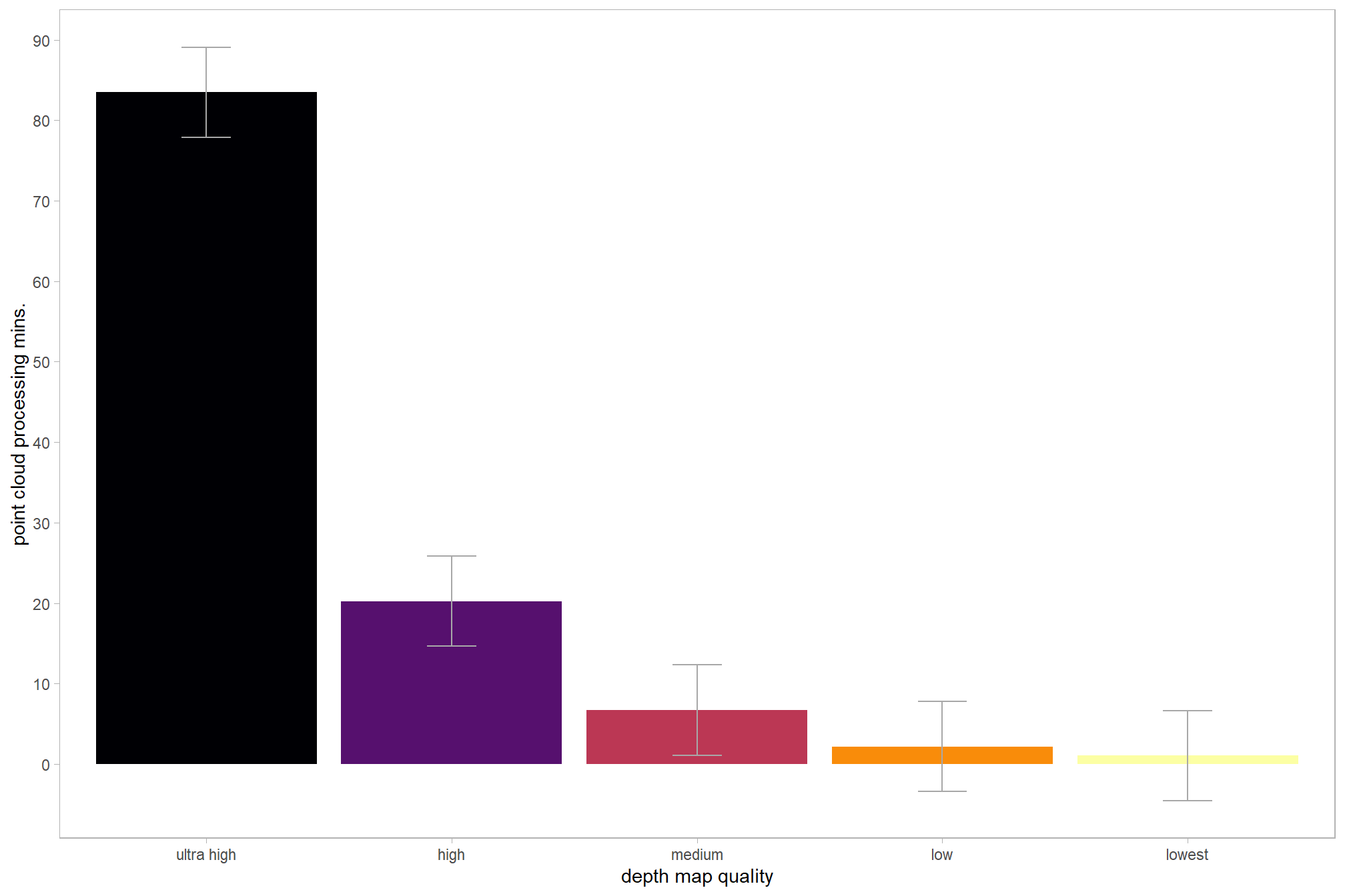
4.1.3 ANOVA
One-way ANOVA to test for differences in group means
aov1_temp = aov(
  timer_total_time_mins ~ 0 + depth_maps_generation_quality
  , data = ptime_data
)
# summary
aov1_temp %>%
  broom::tidy() %>%
  kableExtra::kbl(digits = 2, caption = "one-way ANOVA: point cloud processing time by depth map quality") %>%
kableExtra::kable_styling()| term | df | sumsq | meansq | statistic | p.value |
|---|---|---|---|---|---|
| depth_maps_generation_quality | 5 | 148594.20 | 29718.84 | 186.85 | 0 |
| Residuals | 95 | 15109.77 | 159.05 | NA | NA |
The sum of squared residuals is the same between the linear model and the ANOVA model
# RSS
identical(
  # linear model
  lm1_temp$residuals %>%
    dplyr::as_tibble() %>%
    mutate(value=value^2) %>%
    dplyr::pull(value) %>%
    sum()
  # anova
  , summary(aov1_temp)[[1]][["Sum Sq"]][[2]]
)
## [1] TRUE# F value
identical(
# linear model
summary(lm1_temp)$fstatistic["value"] %>% unname() %>% round(6)
# anova
, summary(aov1_temp)[[1]][["F value"]][[1]] %>% unname() %>% round(6)
)## [1] TRUEwe can use the marginaleffects package to compare and contrast the mean estimates by group.
# calculate average group effects
contrast_temp =
  marginaleffects::avg_comparisons(
    model = lm1_temp
    , variables = list(depth_maps_generation_quality = "revpairwise")
    , comparison = "difference"
  ) %>%
  dplyr::mutate(
    contrast = contrast %>%
      stringr::str_remove_all("mean\\(") %>%
      stringr::str_remove_all("\\)")
  )

# separate contrast
contrast_temp =
  contrast_temp %>%
  tidyr::separate_wider_delim(
    cols = contrast
    , delim = " - "
    , names = paste0(
        "sorter"
        , 1:(max(stringr::str_count(contrast_temp$contrast, "-"))+1)
      )
    , too_few = "align_start"
    , cols_remove = F
  ) %>%
  dplyr::filter(sorter1!=sorter2) %>%
  dplyr::mutate(
    dplyr::across(
      tidyselect::starts_with("sorter")
      , .fns = function(x){factor(
        x, ordered = T
        , levels = levels(ptime_data$depth_maps_generation_quality)
      )}
    )
    , contrast = contrast %>% forcats::fct_reorder(
        paste0(as.numeric(sorter1), as.numeric(sorter2)) %>%
        as.numeric()
      )
    , sig_lvl = dplyr::case_when(
        p.value <= 0.01 ~ "0.01"
        , p.value <= 0.05 ~ "0.05"
        , p.value <= 0.1 ~ "0.10"
        , T ~ "not significant"
      ) %>%
      factor(
        ordered = T
        , levels = c(
          "0.01"
          , "0.05"
          , "0.10"
          , "not significant"
        )
      )
  ) %>%
  dplyr::arrange(contrast)

# plot
contrast_temp %>%
  # plot
  ggplot(mapping = aes(y = contrast)) +
    geom_linerange(
      mapping = aes(xmin = conf.low, xmax = conf.high, color = sig_lvl)
      , linewidth = 5
      , alpha = 0.9
    ) +
    geom_point(mapping = aes(x = estimate)) +
    geom_vline(xintercept = 0, linetype = "dashed", color = "gray44") +
    scale_color_viridis_d(option = "mako", begin = 0.3, drop = F) +
    scale_x_continuous(breaks = scales::extended_breaks(n=8)) +
    labs(
      y = "depth map quality"
      , x = "constrast (mins.)"
      , subtitle = "Mean group constrasts"
      , color = "sig. level"
    ) +
    theme_light() +
    theme(
      legend.position = "top"
      , legend.direction = "horizontal"
    )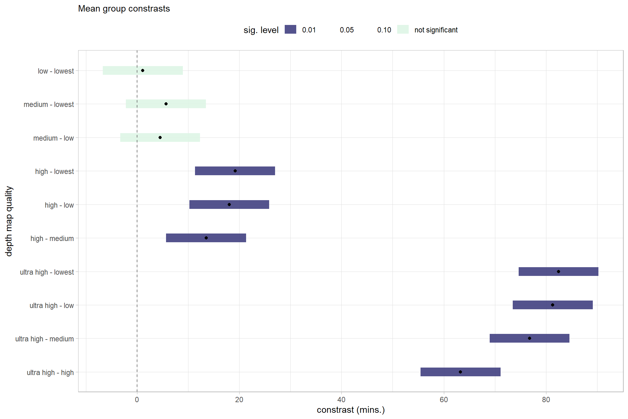
and view the contrasts in a table
contrast_temp %>%
  dplyr::arrange(contrast) %>%
  dplyr::select(contrast, estimate, conf.low, conf.high, p.value) %>%
  dplyr::rename(difference=estimate) %>%
kableExtra::kbl(
    digits = 2, caption = "Mean group effects: depth map quality processing time constrasts"
  ) %>%
  kableExtra::kable_styling() %>%
kableExtra::scroll_box(height = "6in")| contrast | difference | conf.low | conf.high | p.value |
|---|---|---|---|---|
| ultra high - high | 63.27 | 55.46 | 71.09 | 0.00 |
| ultra high - medium | 76.78 | 68.97 | 84.60 | 0.00 |
| ultra high - low | 81.31 | 73.50 | 89.13 | 0.00 |
| ultra high - lowest | 82.45 | 74.63 | 90.26 | 0.00 |
| high - medium | 13.51 | 5.70 | 21.33 | 0.00 |
| high - low | 18.04 | 10.22 | 25.86 | 0.00 |
| high - lowest | 19.18 | 11.36 | 26.99 | 0.00 |
| medium - low | 4.53 | -3.29 | 12.35 | 0.26 |
| medium - lowest | 5.66 | -2.15 | 13.48 | 0.16 |
| low - lowest | 1.14 | -6.68 | 8.95 | 0.78 |
4.1.4 Bayesian
Kruschke (2015) notes:
The terminology, “analysis of variance,” comes from a decomposition of overall data variance into within-group variance and between-group variance (Fisher, 1925). Algebraically, the sum of squared deviations of the scores from their overall mean equals the sum of squared deviations of the scores from their respective group means plus the sum of squared deviations of the group means from the overall mean. In other words, the total variance can be partitioned into within-group variance plus between-group variance. Because one definition of the word “analysis” is separation into constituent parts, the term ANOVA accurately describes the underlying algebra in the traditional methods. That algebraic relation is not used in the hierarchical Bayesian approach presented here. The Bayesian method can estimate component variances, however. Therefore, the Bayesian approach is not ANOVA, but is analogous to ANOVA. (p. 556)
and see section 19 from Kurz’s ebook supplement
The metric predicted variable with one nominal predictor variable model has the form:
\[\begin{align*} y_{i} &\sim {\sf Normal} \bigl(\mu_{i}, \sigma_{y} \bigr) \\ \mu_{i} &= \beta_0 + \sum_{j=1}^{J} \beta_{1[j]} x_{1[j]} \bigl(i\bigr) \\ \beta_{0} &\sim {\sf Normal} (0,10) \\ \beta_{1[j]} &\sim {\sf Normal} (0,\sigma_{\beta_{1}}) \\ \sigma_{\beta_{1}} &\sim {\sf uniform} (0,100) \\ \sigma_{y} &\sim {\sf uniform} (0,100) \\ \end{align*}\]
, where \(j\) is the depth map generation quality setting corresponding to observation \(i\)
to start, we’ll use the default brms::brm prior settings which may not match those described in the model specification above
brms1_mod = brms::brm(
formula = timer_total_time_mins ~ 1 + (1 | depth_maps_generation_quality)
, data = ptime_data
, family = brms::brmsfamily(family = "gaussian")
, iter = 3000, warmup = 1000, chains = 4
, cores = round(parallel::detectCores()/2)
, file = paste0(rootdir, "/fits/brms1_mod")
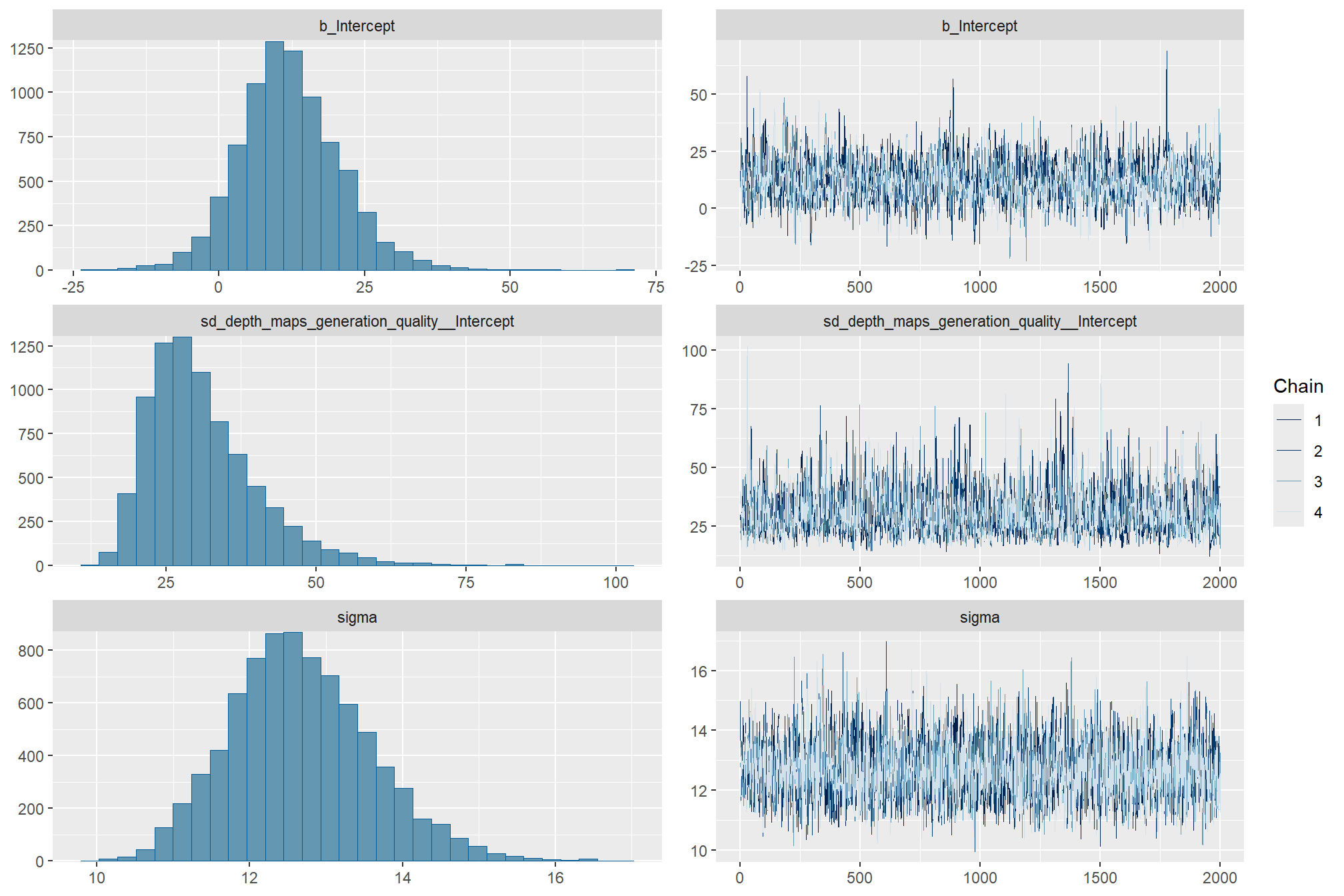
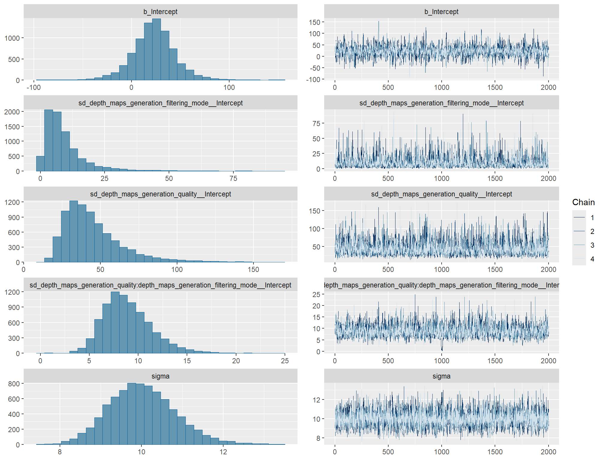
)check the trace plots for problems with convergence of the Markov chains
check the prior distributions
| prior | class | coef | group | resp | dpar | nlpar | lb | ub | source |
|---|---|---|---|---|---|---|---|---|---|
| student_t(3, 6.6, 8.2) | Intercept | default | |||||||
| student_t(3, 0, 8.2) | sd | 0 | default | ||||||
| sd | depth_maps_generation_quality | default | |||||||
| sd | Intercept | depth_maps_generation_quality | default | ||||||
| student_t(3, 0, 8.2) | sigma | 0 | default |
The brms::brm model summary
brms1_mod %>%
  brms::posterior_summary() %>%
  as.data.frame() %>%
  tibble::rownames_to_column(var = "parameter") %>%
  dplyr::rename_with(tolower) %>%
  dplyr::filter(
    stringr::str_starts(parameter, "b_")
    | stringr::str_starts(parameter, "r_")
    | parameter == "sigma"
  ) %>%
  dplyr::mutate(
    parameter = parameter %>%
      stringr::str_remove_all("b_depth_maps_generation_quality") %>%
      stringr::str_remove_all("r_depth_maps_generation_quality")
  ) %>%
  kableExtra::kbl(digits = 2, caption = "Bayesian one nominal predictor: point cloud processing time by depth map quality") %>%
kableExtra::kable_styling()| parameter | estimate | est.error | q2.5 | q97.5 |
|---|---|---|---|---|
| b_Intercept | 12.09 | 8.69 | -3.91 | 30.55 |
| sigma | 12.67 | 0.93 | 11.00 | 14.65 |
| [ultra.high,Intercept] | 70.66 | 9.13 | 51.67 | 87.34 |
| [high,Intercept] | 8.10 | 9.15 | -10.79 | 25.05 |
| [medium,Intercept] | -5.33 | 9.00 | -24.25 | 11.58 |
| [low,Intercept] | -9.81 | 9.09 | -28.62 | 7.16 |
| [lowest,Intercept] | -10.87 | 9.10 | -29.81 | 5.89 |
With the stats::coef function, we can get the group-level summaries in a “non-deflection” metric. In the model, the group means represented by \(\beta_{1[j]}\) are deflections from overall baseline, such that the deflections sum to zero (see Kruschke (2015, p.554)). Summaries of the group-specific deflections are available via the brms::ranef function.
stats::coef(brms1_mod) %>%
  as.data.frame() %>%
  tibble::rownames_to_column(var = "group") %>%
  dplyr::rename_with(
    .cols = -c("group")
    , .fn = ~ stringr::str_remove_all(.x, "depth_maps_generation_quality.")
  ) %>%
  kableExtra::kbl(digits = 2, caption = "brms::brm model: point cloud processing time by depth map quality") %>%
kableExtra::kable_styling()| group | Estimate.Intercept | Est.Error.Intercept | Q2.5.Intercept | Q97.5.Intercept |
|---|---|---|---|---|
| ultra high | 82.75 | 2.90 | 76.96 | 88.42 |
| high | 20.19 | 2.85 | 14.58 | 25.77 |
| medium | 6.76 | 2.88 | 1.02 | 12.36 |
| low | 2.28 | 2.90 | -3.45 | 7.92 |
| lowest | 1.21 | 2.85 | -4.33 | 6.81 |
We can look at the model noise standard deviation \(\sigma_y\)
# extract the posterior draws
brms::as_draws_df(brms1_mod) %>%
# plot
  ggplot(aes(x = sigma, y = 0)) +
  tidybayes::stat_dotsinterval(
    point_interval = median_hdi, .width = .95
    , justification = -0.04
    , shape = 21, point_size = 3
    , quantiles = 100
  ) +
  scale_y_continuous(NULL, breaks = NULL) +
  xlab(latex2exp::TeX("$\\sigma_y$")) +
  theme_light()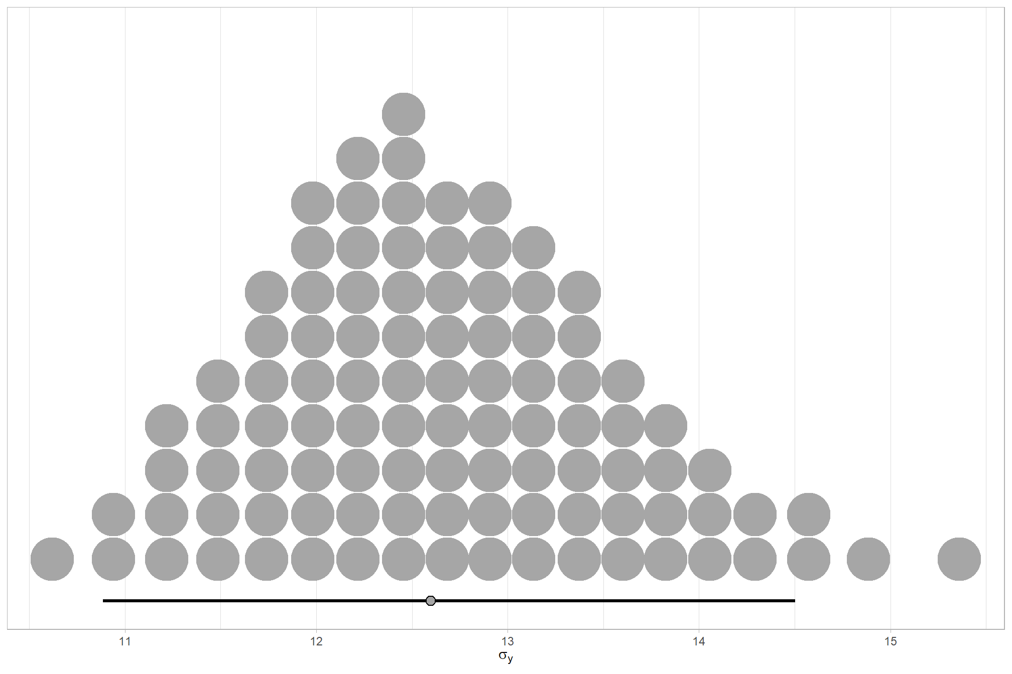
plot the posterior distributions of the conditional means with the median processing time and the 95% highest posterior density interval (HDI)
ptime_data %>%
  dplyr::distinct(depth_maps_generation_quality) %>%
  tidybayes::add_epred_draws(brms1_mod) %>%
  dplyr::mutate(value = .epred) %>%
  # plot
  ggplot(
    mapping = aes(
      x = value, y = depth_maps_generation_quality
      , fill = depth_maps_generation_quality
    )
  ) +
    tidybayes::stat_halfeye(
      point_interval = median_hdi, .width = .95
      , interval_color = "gray66"
      , shape = 21, point_color = "gray66", point_fill = "black"
      , justification = -0.01
    ) +
    # tidybayes::stat_dotsinterval(
    #   point_interval = median_hdi, .width = .95
    #   , shape = 21, point_fill = "gray", justification = -0.04
    #   , quantiles = 100
    # ) +
    scale_fill_viridis_d(option = "inferno", drop = F) +
    scale_x_continuous(breaks = scales::extended_breaks(n=8)) +
    labs(
      y = "depth map quality", x = "point cloud processing mins."
      , subtitle = "posterior distribution of conditional means with 95% HDI"
    ) +
    theme_light() +
    theme(legend.position = "none")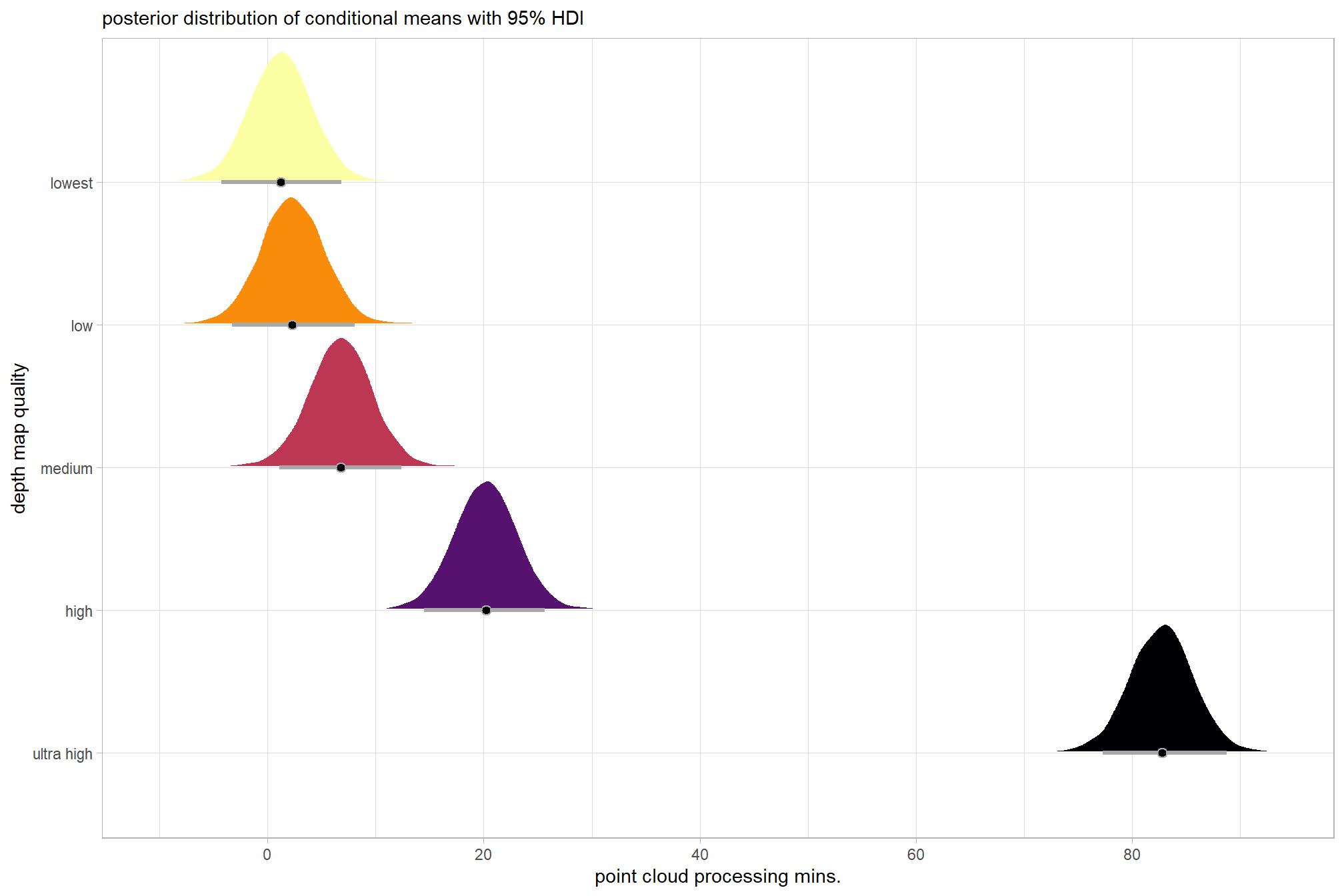
we can also make pairwise comparisons
# define comparisons to make
contrast_temp = contrast_temp %>% dplyr::arrange(contrast)
contrast_list =
  1:nrow(contrast_temp) %>%
  purrr::map(function(x){
    c(contrast_temp$sorter1[x],contrast_temp$sorter2[x])
  }) %>%
  list() %>%
  purrr::list_flatten()

# obtain posterior draws and calculate contrasts using tidybayes::compare_levels
brms_contrast_temp =
  brms1_mod %>%
    tidybayes::spread_draws(r_depth_maps_generation_quality[depth_maps_generation_quality]) %>%
    dplyr::mutate(
      depth_maps_generation_quality = depth_maps_generation_quality %>%
        stringr::str_replace_all("\\.", " ") %>%
        factor(
          levels = levels(ptime_data$depth_maps_generation_quality)
          , ordered = T
        )
    ) %>%
    dplyr::rename(value = r_depth_maps_generation_quality) %>%
    tidybayes::compare_levels(
      value
      , by = depth_maps_generation_quality
      , comparison =
        contrast_list
        # tidybayes::emmeans_comparison("revpairwise")
        #"pairwise"
    ) %>%
    dplyr::mutate(
      contrast = depth_maps_generation_quality %>%
        factor(
          levels = levels(contrast_temp$contrast)
          , ordered = T
        )
    )

# median_hdi summary for coloring
brms_contrast_temp = brms_contrast_temp %>%
  dplyr::inner_join(
    brms_contrast_temp %>%
      dplyr::group_by(contrast) %>%
      tidybayes::median_hdi(value, .width = c(0.5,0.95)) %>%
      dplyr::mutate(
        sig_level = dplyr::case_when(
          .lower<0 & .upper>0 ~ 1
          , T ~ 0
        )
      ) %>%
      dplyr::select(.width,sig_level,contrast) %>%
      tidyr::pivot_wider(names_from = .width, values_from = sig_level) %>%
      dplyr::mutate(
        sig_level = dplyr::case_when(
          `0.5` == 1 ~ 0
          , `0.95` == 1 ~ 1
          , T ~ 2
        ) %>%
        factor(levels = c(0,1,2), labels = c("50%","5%","0%")) %>%
        forcats::fct_rev()
      ) %>%
      dplyr::select(contrast, sig_level)
    , by = dplyr::join_by(contrast)
  ) %>%
  dplyr::group_by(contrast) %>%
  dplyr::mutate(
    is_gt_zero = value > 0
    , pct_gt_zero = sum(is_gt_zero)/dplyr::n()
    , sig_level2 = dplyr::case_when(
      pct_gt_zero > 0.99 ~ 0
      , pct_gt_zero > 0.95 ~ 1
      , pct_gt_zero > 0.9 ~ 2
      , pct_gt_zero > 0.8 ~ 3
      , T ~ 4
    ) %>%
    factor(levels = c(0:4), labels = c(">99%","95%","90%","80%","<80%"), ordered = T)
  )
# what?
brms_contrast_temp %>% dplyr::glimpse()
## Rows: 80,000
## Columns: 10
## Groups: contrast [10]
## $ .chain <int> 1, 1, 1, 1, 1, 1, 1, 1, 1, 1, 1, 1, 1, 1…
## $ .iteration <int> 1, 2, 3, 4, 5, 6, 7, 8, 9, 10, 11, 12, 1…
## $ .draw <int> 1, 2, 3, 4, 5, 6, 7, 8, 9, 10, 11, 12, 1…
## $ depth_maps_generation_quality <chr> "ultra high - high", "ultra high - high"…
## $ value <dbl> 58.31630, 69.37204, 54.19820, 60.82334, …
## $ contrast <ord> ultra high - high, ultra high - high, ul…
## $ sig_level <fct> 0%, 0%, 0%, 0%, 0%, 0%, 0%, 0%, 0%, 0%, …
## $ is_gt_zero <lgl> TRUE, TRUE, TRUE, TRUE, TRUE, TRUE, TRUE…
## $ pct_gt_zero <dbl> 1, 1, 1, 1, 1, 1, 1, 1, 1, 1, 1, 1, 1, 1…
## $ sig_level2 <ord> >99%, >99%, >99%, >99%, >99%, >99%, >99%…plot it
# plot, finally
brms_contrast_temp %>%
  ggplot(aes(x = value, y = contrast, fill = sig_level2)) +
    tidybayes::stat_halfeye(
      point_interval = median_hdi, .width = c(0.5,0.95)
      # , slab_fill = "gray22", slab_alpha = 1
      , interval_color = "black", point_color = "black", point_fill = "black"
      , justification = -0.01
    ) +
    geom_vline(xintercept = 0, linetype = "dashed", color = "gray44") +
    scale_fill_viridis_d(
      option = "mako", begin = 0.3
      , drop = F
      # , labels = scales::percent
    ) +
    scale_x_continuous(breaks = scales::extended_breaks(n=8)) +
    labs(
      y = "depth map quality"
      , x = "constrast (mins.)"
      , fill = "Pr(contrast > 0)"
      , subtitle = "95% & 50% HDI of the posterior distribution of conditional mean group constrasts"
    ) +
    theme_light() +
    theme(legend.position = "top", legend.direction = "horizontal") +
    guides(
      fill = guide_legend(reverse = T, override.aes = list(alpha = 1, color = NA, shape = NA, lwd = NA))
    )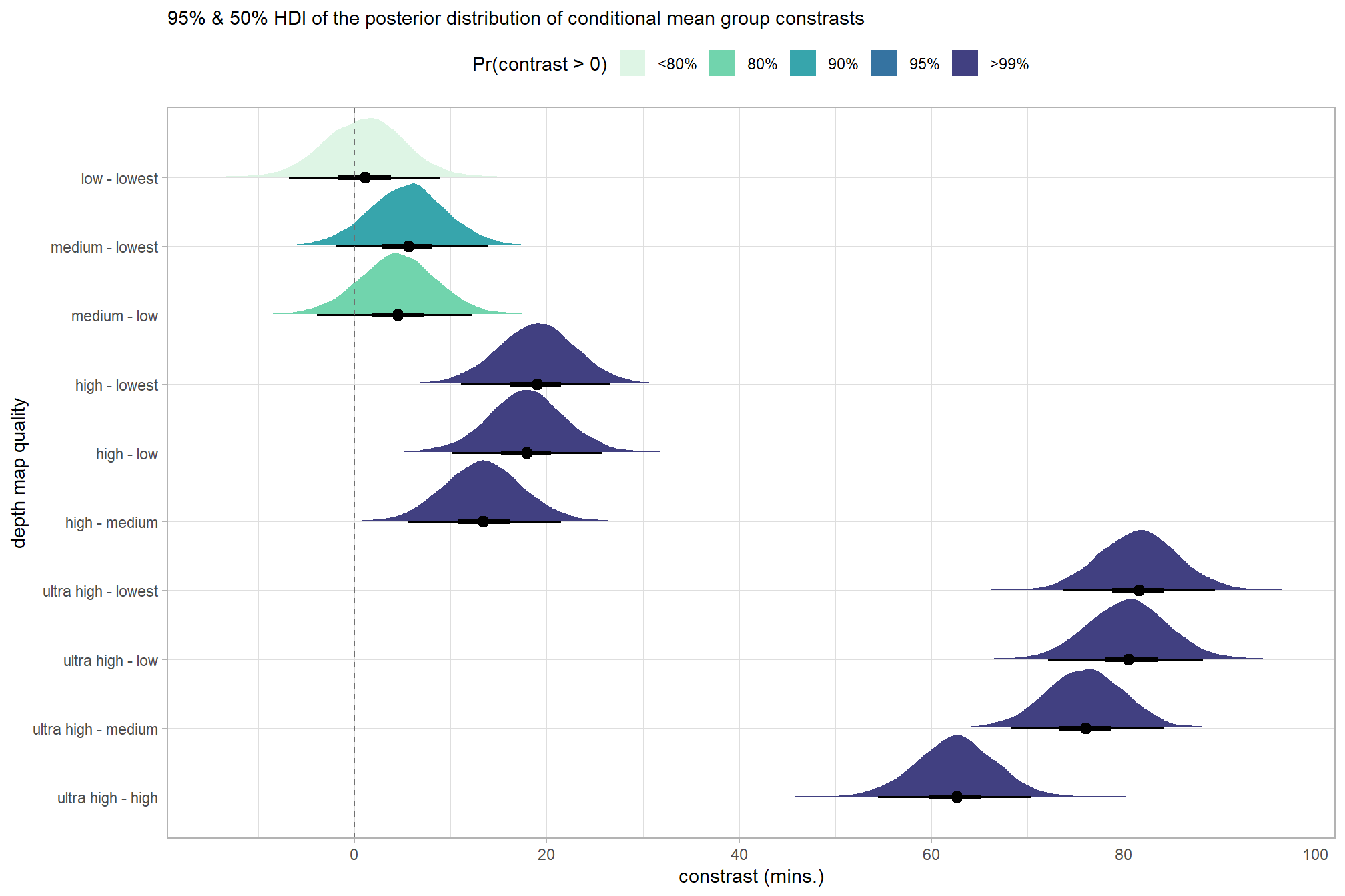
and summarize these contrasts
# # can also use the following as substitute for the "tidybayes::spread_draws" used above to get same result
brms_contrast_temp %>%
  dplyr::group_by(contrast) %>%
  tidybayes::median_hdi(value) %>%
  select(-c(.point,.interval)) %>%
  dplyr::arrange(desc(contrast)) %>%
  dplyr::rename(difference=value) %>%
  kableExtra::kbl(digits = 1, caption = "brms::brm model: 95% HDI of the posterior distribution of conditional mean group constrasts") %>%
kableExtra::kable_styling()| contrast | difference | .lower | .upper | .width |
|---|---|---|---|---|
| low - lowest | 1.1 | -6.8 | 8.9 | 0.9 |
| medium - lowest | 5.6 | -2.0 | 13.9 | 0.9 |
| medium - low | 4.5 | -3.9 | 12.3 | 0.9 |
| high - lowest | 19.0 | 11.1 | 26.7 | 0.9 |
| high - low | 17.9 | 10.1 | 25.8 | 0.9 |
| high - medium | 13.4 | 5.6 | 21.5 | 0.9 |
| ultra high - lowest | 81.6 | 73.6 | 89.5 | 0.9 |
| ultra high - low | 80.5 | 72.1 | 88.2 | 0.9 |
| ultra high - medium | 76.0 | 68.2 | 84.1 | 0.9 |
| ultra high - high | 62.6 | 54.5 | 70.4 | 0.9 |
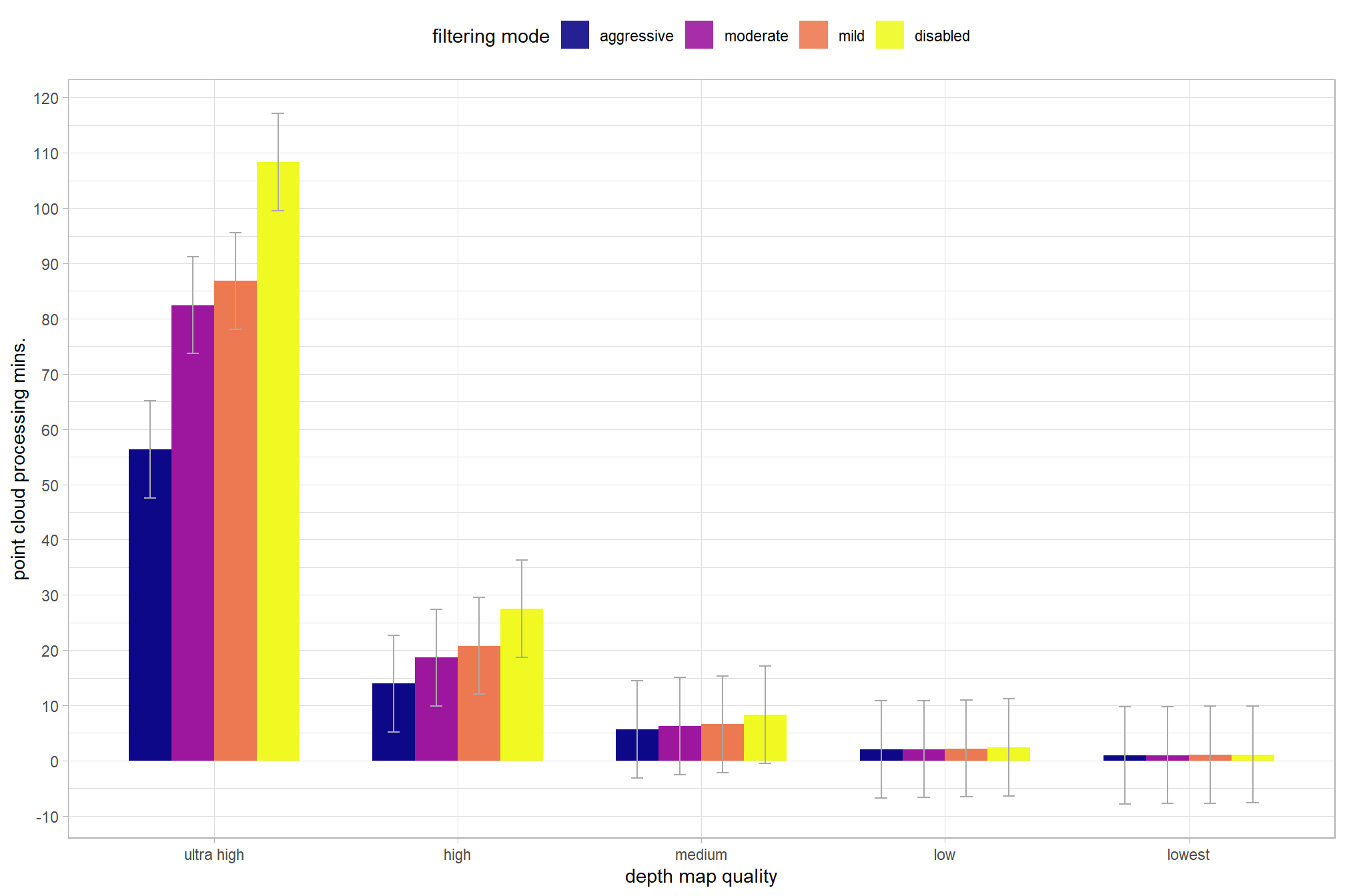
4.2 Two Nominal Predictors
Now, we’ll determine the combined influence of the depth map generation quality and the depth map filtering parameters on the point cloud processing time.
4.2.1 Summary Statistics
Summary statistics by group:
ptime_data %>%
  dplyr::group_by(depth_maps_generation_quality, depth_maps_generation_filtering_mode) %>%
  dplyr::summarise(
    mean_processing_mins = mean(timer_total_time_mins, na.rm = T)
    # , med_processing_mins = median(timer_total_time_mins, na.rm = T)
    , sd_processing_mins = sd(timer_total_time_mins, na.rm = T)
    , n = dplyr::n()
  ) %>%
  kableExtra::kbl(
    digits = 1
    , caption = "summary statistics: point cloud processing time by depth map quality and filtering mode"
    , col.names = c(
      "depth map quality"
      , "filtering mode"
      , "mean time"
      , "sd"
      , "n"
    )
  ) %>%
  kableExtra::kable_styling() %>%
kableExtra::scroll_box(height = "6in")| depth map quality | filtering mode | mean time | sd | n |
|---|---|---|---|---|
| ultra high | aggressive | 56.3 | 14.8 | 5 |
| ultra high | moderate | 82.5 | 19.7 | 5 |
| ultra high | mild | 86.8 | 20.0 | 5 |
| ultra high | disabled | 108.3 | 29.5 | 5 |
| high | aggressive | 13.9 | 3.3 | 5 |
| high | moderate | 18.6 | 3.2 | 5 |
| high | mild | 20.8 | 4.7 | 5 |
| high | disabled | 27.5 | 3.5 | 5 |
| medium | aggressive | 5.7 | 1.3 | 5 |
| medium | moderate | 6.3 | 1.2 | 5 |
| medium | mild | 6.6 | 1.7 | 5 |
| medium | disabled | 8.3 | 1.4 | 5 |
| low | aggressive | 2.0 | 0.2 | 5 |
| low | moderate | 2.1 | 0.3 | 5 |
| low | mild | 2.2 | 0.2 | 5 |
| low | disabled | 2.4 | 0.3 | 5 |
| lowest | aggressive | 1.0 | 0.1 | 5 |
| lowest | moderate | 1.0 | 0.1 | 5 |
| lowest | mild | 1.1 | 0.1 | 5 |
| lowest | disabled | 1.1 | 0.2 | 5 |
4.2.2 Linear Model
We can use a linear model to obtain means by group:
lm2_temp = lm(
  timer_total_time_mins ~ 1 +
    depth_maps_generation_quality +
    depth_maps_generation_filtering_mode +
    depth_maps_generation_quality:depth_maps_generation_filtering_mode
  , data = ptime_data
)
# summary
predict(
    lm2_temp
    , newdata = ptime_data %>%
        dplyr::distinct(depth_maps_generation_quality, depth_maps_generation_filtering_mode)
    , interval = "confidence"
  ) %>%
  dplyr::as_tibble() %>%
  dplyr::bind_cols(
    ptime_data %>%
      dplyr::distinct(depth_maps_generation_quality, depth_maps_generation_filtering_mode)
  ) %>%
  dplyr::relocate(depth_maps_generation_quality, depth_maps_generation_filtering_mode) %>%
  dplyr::arrange(depth_maps_generation_quality, depth_maps_generation_filtering_mode) %>%
  kableExtra::kbl(
    digits = 1
    , caption = "linear model: point cloud processing time by depth map quality and filtering mode"
    , col.names = c(
      "depth map quality"
      , "filtering mode"
      , "y_hat"
      , "q2.5"
      , "q97.5"
    )
  ) %>%
  kableExtra::kable_styling() %>%
kableExtra::scroll_box(height = "6in")| depth map quality | filtering mode | y_hat | q2.5 | q97.5 |
|---|---|---|---|---|
| ultra high | aggressive | 56.3 | 47.6 | 65.1 |
| ultra high | moderate | 82.5 | 73.7 | 91.2 |
| ultra high | mild | 86.8 | 78.1 | 95.6 |
| ultra high | disabled | 108.3 | 99.6 | 117.1 |
| high | aggressive | 13.9 | 5.2 | 22.7 |
| high | moderate | 18.6 | 9.9 | 27.4 |
| high | mild | 20.8 | 12.0 | 29.5 |
| high | disabled | 27.5 | 18.7 | 36.3 |
| medium | aggressive | 5.7 | -3.1 | 14.4 |
| medium | moderate | 6.3 | -2.5 | 15.0 |
| medium | mild | 6.6 | -2.2 | 15.4 |
| medium | disabled | 8.3 | -0.5 | 17.1 |
| low | aggressive | 2.0 | -6.7 | 10.8 |
| low | moderate | 2.1 | -6.7 | 10.8 |
| low | mild | 2.2 | -6.6 | 11.0 |
| low | disabled | 2.4 | -6.4 | 11.2 |
| lowest | aggressive | 1.0 | -7.8 | 9.7 |
| lowest | moderate | 1.0 | -7.8 | 9.8 |
| lowest | mild | 1.1 | -7.7 | 9.8 |
| lowest | disabled | 1.1 | -7.6 | 9.9 |
and plot these means with 95% confidence interval
predict(
    lm2_temp
    , newdata = ptime_data %>%
        dplyr::distinct(depth_maps_generation_quality, depth_maps_generation_filtering_mode)
    , interval = "confidence"
  ) %>%
  dplyr::as_tibble() %>%
  dplyr::bind_cols(
    ptime_data %>%
      dplyr::distinct(depth_maps_generation_quality, depth_maps_generation_filtering_mode)
  ) %>%
  ggplot(
    mapping = aes(
      y = fit
      , x = depth_maps_generation_quality
      , fill = depth_maps_generation_filtering_mode
      , group = depth_maps_generation_filtering_mode
    )
  ) +
  geom_col(width = 0.7, position = "dodge") +
  geom_errorbar(
    mapping = aes(ymin = lwr, ymax = upr)
    , width = 0.2, color = "gray66"
    , position = position_dodge(width = 0.7)
  ) +
  scale_fill_viridis_d(option = "plasma", drop = F) +
  scale_y_continuous(breaks = scales::extended_breaks(n=14)) +
  labs(
    fill = "filtering mode"
    , x = "depth map quality"
    , y = "point cloud processing mins."
  ) +
  theme_light() +
  theme(
    legend.position = "top"
    , legend.direction  = "horizontal"
  ) +
  guides(
    fill = guide_legend(override.aes = list(alpha = 0.9))
  )
4.2.3 ANOVA
ANOVA to test for differences in group means
aov2_temp = aov(
  timer_total_time_mins ~ 1 +
    depth_maps_generation_quality +
    depth_maps_generation_filtering_mode +
    depth_maps_generation_quality:depth_maps_generation_filtering_mode
  , data = ptime_data
)
# summary
aov2_temp %>%
  broom::tidy() %>%
  kableExtra::kbl(digits = 2, caption = "two-way ANOVA: point cloud processing time by depth map quality and filtering mode") %>%
kableExtra::kable_styling()| term | df | sumsq | meansq | statistic | p.value |
|---|---|---|---|---|---|
| depth_maps_generation_quality | 4 | 96952.48 | 24238.12 | 249.35 | 0 |
| depth_maps_generation_filtering_mode | 3 | 2387.66 | 795.89 | 8.19 | 0 |
| depth_maps_generation_quality:depth_maps_generation_filtering_mode | 12 | 4945.59 | 412.13 | 4.24 | 0 |
| Residuals | 80 | 7776.52 | 97.21 | NA | NA |
We can perform pairwise comparisons of the filtering mode between at each depth map quality level
# Pairwise comparisons between group levels
ptime_data %>%
  group_by(depth_maps_generation_quality) %>%
  rstatix::pairwise_t_test(
    timer_total_time_mins ~ depth_maps_generation_filtering_mode
    , p.adjust.method = "bonferroni"
  ) %>%
  dplyr::select(-c(n1,p,p.signif,.y.)) %>%
  kableExtra::kbl(
    digits = 1
    , caption = "Pairwise comparisons between filtering mode at each depth map quality group"
  ) %>%
  kableExtra::kable_styling() %>%
kableExtra::scroll_box(height = "6in")| depth_maps_generation_quality | group1 | group2 | n2 | p.adj | p.adj.signif |
|---|---|---|---|---|---|
| ultra high | aggressive | moderate | 5 | 0.4 | ns |
| ultra high | aggressive | mild | 5 | 0.2 | ns |
| ultra high | moderate | mild | 5 | 1.0 | ns |
| ultra high | aggressive | disabled | 5 | 0.0 | ** |
| ultra high | moderate | disabled | 5 | 0.5 | ns |
| ultra high | mild | disabled | 5 | 0.8 | ns |
| high | aggressive | moderate | 5 | 0.4 | ns |
| high | aggressive | mild | 5 | 0.1 | ns |
| high | moderate | mild | 5 | 1.0 | ns |
| high | aggressive | disabled | 5 | 0.0 | *** |
| high | moderate | disabled | 5 | 0.0 |
|
| high | mild | disabled | 5 | 0.1 | ns |
| medium | aggressive | moderate | 5 | 1.0 | ns |
| medium | aggressive | mild | 5 | 1.0 | ns |
| medium | moderate | mild | 5 | 1.0 | ns |
| medium | aggressive | disabled | 5 | 0.1 | ns |
| medium | moderate | disabled | 5 | 0.2 | ns |
| medium | mild | disabled | 5 | 0.4 | ns |
| low | aggressive | moderate | 5 | 1.0 | ns |
| low | aggressive | mild | 5 | 1.0 | ns |
| low | moderate | mild | 5 | 1.0 | ns |
| low | aggressive | disabled | 5 | 0.3 | ns |
| low | moderate | disabled | 5 | 0.5 | ns |
| low | mild | disabled | 5 | 1.0 | ns |
| lowest | aggressive | moderate | 5 | 1.0 | ns |
| lowest | aggressive | mild | 5 | 1.0 | ns |
| lowest | moderate | mild | 5 | 1.0 | ns |
| lowest | aggressive | disabled | 5 | 0.3 | ns |
| lowest | moderate | disabled | 5 | 0.7 | ns |
| lowest | mild | disabled | 5 | 1.0 | ns |
we can use the emmeans package to perform interaction analysis of the mean estimates using Tukey’s Honest Significant Differences method.
we can use the marginaleffects package to compare and contrast the mean estimates by group.
# calculate average group effects
# ... for a "cross-contrast" use cross = T (code below) where...
# ......contrasts represent the changes in adjusted predictions when
# ......all the predictors specified in the variables argument are manipulated simultaneously
# avg_comparisons(mod, variables = c("cyl", "gear"), cross = TRUE)
contrast_temp =
  marginaleffects::avg_comparisons(
    model = lm2_temp
    , variables = list(depth_maps_generation_quality = "revpairwise")
    , comparison = "difference"
    , by = "depth_maps_generation_filtering_mode"
  ) %>%
  dplyr::mutate(
    contrast = contrast %>%
      stringr::str_remove_all("mean\\(") %>%
      stringr::str_remove_all("\\)")
  )

# separate contrast
contrast_temp = contrast_temp %>%
  dplyr::mutate(
    contrast = contrast %>%
      stringr::str_remove_all("mean\\(") %>%
      stringr::str_remove_all("\\)")
  ) %>%
  tidyr::separate_wider_delim(
    cols = contrast
    , delim = " - "
    , names = paste0(
        "sorter"
        , 1:(max(stringr::str_count(contrast_temp$contrast, "-"))+1)
      )
    , too_few = "align_start"
    , cols_remove = F
  ) %>%
  dplyr::filter(sorter1!=sorter2) %>%
  dplyr::mutate(
    dplyr::across(
      tidyselect::starts_with("sorter")
      , .fns = function(x){factor(
        x, ordered = T
        , levels = levels(ptime_data$depth_maps_generation_quality)
      )}
    )
    , contrast = contrast %>% forcats::fct_reorder(
        paste0(as.numeric(sorter1), as.numeric(sorter2)) %>%
        as.numeric()
      )
    , sig_lvl = dplyr::case_when(
        p.value <= 0.01 ~ "0.01"
        , p.value <= 0.05 ~ "0.05"
        , p.value <= 0.1 ~ "0.10"
        , T ~ "not significant"
      ) %>%
      factor(
        ordered = T
        , levels = c(
          "0.01"
          , "0.05"
          , "0.10"
          , "not significant"
        )
      )
    , depth_maps_generation_filtering_mode = depth_maps_generation_filtering_mode %>%
      factor(
        ordered = T
        , levels = levels(ptime_data$depth_maps_generation_filtering_mode)
      )
  ) %>%
  dplyr::arrange(contrast, depth_maps_generation_filtering_mode)

# what?
contrast_temp %>% dplyr::ungroup() %>% dplyr::glimpse()
## Rows: 40
## Columns: 16
## $ term <chr> "depth_maps_generation_quality", …
## $ sorter1 <ord> ultra high, ultra high, ultra hig…
## $ sorter2 <ord> high, high, high, high, medium, m…
## $ contrast <fct> ultra high - high, ultra high - h…
## $ depth_maps_generation_filtering_mode <ord> aggressive, moderate, mild, disab…
## $ estimate <dbl> 42.39916, 63.80675, 66.06454, 80.…
## $ std.error <dbl> 6.235593, 6.235587, 6.235590, 6.2…
## $ statistic <dbl> 6.799539, 10.232677, 10.594754, 1…
## $ p.value <dbl> 1.049541e-11, 1.415513e-24, 3.151…
## $ s.value <dbl> 36.471450, 79.224949, 84.714012, …
## $ conf.low <dbl> 30.1776215, 51.5852240, 53.843009…
## $ conf.high <dbl> 54.62070, 76.02828, 78.28607, 93.…
## $ predicted_lo <dbl> 13.9287619, 18.6492584, 20.771895…
## $ predicted_hi <dbl> 56.32792, 82.45601, 86.83644, 108…
## $ predicted <dbl> 13.92876, 18.64926, 20.77190, 27.…
## $ sig_lvl <ord> 0.01, 0.01, 0.01, 0.01, 0.01, 0.0…plot it
contrast_temp %>%
  # plot
  ggplot(mapping = aes(y = contrast)) +
    geom_linerange(
      mapping = aes(xmin = conf.low, xmax = conf.high, color = sig_lvl)
      , linewidth = 5
      , alpha = 0.9
    ) +
    geom_point(mapping = aes(x = estimate)) +
    geom_vline(xintercept = 0, linetype = "dashed", color = "gray44") +
    scale_color_viridis_d(option = "mako", begin = 0.3, drop = F) +
    scale_x_continuous(breaks = scales::extended_breaks(n=8)) +
    facet_grid(cols = vars(depth_maps_generation_filtering_mode)) +
    labs(
      y = "depth map quality"
      , x = "constrast (mins.)"
      , subtitle = "Mean group constrasts"
      , color = "sig. level"
    ) +
    theme_light() +
    theme(
      legend.position = "top"
      , legend.direction = "horizontal"
      , strip.text = element_text(color = "black", face = "bold")
    )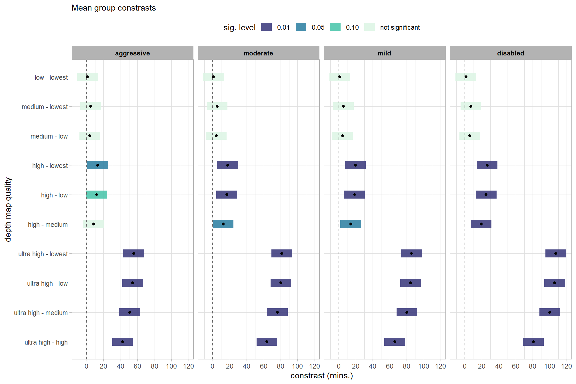
and view the contrasts in a table
contrast_temp %>%
  dplyr::arrange(contrast, depth_maps_generation_filtering_mode) %>%
  dplyr::select(contrast, depth_maps_generation_filtering_mode, estimate, conf.low, conf.high, p.value) %>%
  dplyr::rename(difference=estimate) %>%
kableExtra::kbl(
    digits = 2, caption = "Mean group effects: depth map quality processing time constrasts"
    , col.names = c(
      "quality contrast"
      , "filtering mode"
      , "difference (mins.)"
      , "conf.low", "conf.high", "p.value"
    )
  ) %>%
  kableExtra::kable_styling() %>%
kableExtra::scroll_box(height = "6in")| quality contrast | filtering mode | difference (mins.) | conf.low | conf.high | p.value |
|---|---|---|---|---|---|
| ultra high - high | aggressive | 42.40 | 30.18 | 54.62 | 0.00 |
| ultra high - high | moderate | 63.81 | 51.59 | 76.03 | 0.00 |
| ultra high - high | mild | 66.06 | 53.84 | 78.29 | 0.00 |
| ultra high - high | disabled | 80.82 | 68.60 | 93.04 | 0.00 |
| ultra high - medium | aggressive | 50.67 | 38.44 | 62.89 | 0.00 |
| ultra high - medium | moderate | 76.18 | 63.96 | 88.40 | 0.00 |
| ultra high - medium | mild | 80.25 | 68.03 | 92.48 | 0.00 |
| ultra high - medium | disabled | 100.03 | 87.81 | 112.26 | 0.00 |
| ultra high - low | aggressive | 54.29 | 42.07 | 66.51 | 0.00 |
| ultra high - low | moderate | 80.38 | 68.16 | 92.61 | 0.00 |
| ultra high - low | mild | 84.63 | 72.41 | 96.85 | 0.00 |
| ultra high - low | disabled | 105.95 | 93.73 | 118.17 | 0.00 |
| ultra high - lowest | aggressive | 55.37 | 43.15 | 67.59 | 0.00 |
| ultra high - lowest | moderate | 81.45 | 69.23 | 93.67 | 0.00 |
| ultra high - lowest | mild | 85.77 | 73.55 | 98.00 | 0.00 |
| ultra high - lowest | disabled | 107.20 | 94.98 | 119.42 | 0.00 |
| high - medium | aggressive | 8.27 | -3.95 | 20.49 | 0.18 |
| high - medium | moderate | 12.37 | 0.15 | 24.60 | 0.05 |
| high - medium | mild | 14.19 | 1.97 | 26.41 | 0.02 |
| high - medium | disabled | 19.22 | 7.00 | 31.44 | 0.00 |
| high - low | aggressive | 11.89 | -0.33 | 24.11 | 0.06 |
| high - low | moderate | 16.58 | 4.36 | 28.80 | 0.01 |
| high - low | mild | 18.57 | 6.34 | 30.79 | 0.00 |
| high - low | disabled | 25.13 | 12.91 | 37.35 | 0.00 |
| high - lowest | aggressive | 12.97 | 0.75 | 25.19 | 0.04 |
| high - lowest | moderate | 17.65 | 5.42 | 29.87 | 0.00 |
| high - lowest | mild | 19.71 | 7.49 | 31.93 | 0.00 |
| high - lowest | disabled | 26.38 | 14.16 | 38.60 | 0.00 |
| medium - low | aggressive | 3.62 | -8.60 | 15.84 | 0.56 |
| medium - low | moderate | 4.20 | -8.02 | 16.42 | 0.50 |
| medium - low | mild | 4.38 | -7.85 | 16.60 | 0.48 |
| medium - low | disabled | 5.91 | -6.31 | 18.14 | 0.34 |
| medium - lowest | aggressive | 4.70 | -7.52 | 16.92 | 0.45 |
| medium - lowest | moderate | 5.27 | -6.95 | 17.49 | 0.40 |
| medium - lowest | mild | 5.52 | -6.70 | 17.74 | 0.38 |
| medium - lowest | disabled | 7.16 | -5.06 | 19.39 | 0.25 |
| low - lowest | aggressive | 1.08 | -11.14 | 13.30 | 0.86 |
| low - lowest | moderate | 1.07 | -11.15 | 13.29 | 0.86 |
| low - lowest | mild | 1.14 | -11.08 | 13.37 | 0.85 |
| low - lowest | disabled | 1.25 | -10.97 | 13.47 | 0.84 |
4.2.4 Bayesian
Kruschke (2015) describes the Hierarchical Bayesian approach to describe groups of metric data with multiple nominal predictors:
This chapter considers data structures that consist of a metric predicted variable and two (or more) nominal predictors….The traditional treatment of this sort of data structure is called multifactor analysis of variance (ANOVA). Our Bayesian approach will be a hierarchical generalization of the traditional ANOVA model. The chapter also considers generalizations of the traditional models, because it is straight forward in Bayesian software to implement heavy-tailed distributions to accommodate outliers, along with hierarchical structure to accommodate heterogeneous variances in the different groups. (pp. 583–584)
and see section 20 from Kurz’s ebook supplement
The metric predicted variable with two nominal predictor variables model has the form:
\[\begin{align*} y_{i} &\sim {\sf Normal} \bigl(\mu_{i}, \sigma_{y} \bigr) \\ \mu_{i} &= \beta_0 + \sum_{j} \beta_{1[j]} x_{1[j]} + \sum_{k} \beta_{2[k]} x_{2[k]} + \sum_{j,k} \beta_{1\times2[j,k]} x_{1\times2[j,k]} \\ \beta_{0} &\sim {\sf Normal} (0,100) \\ \beta_{1[j]} &\sim {\sf Normal} (0,\sigma_{\beta_{1}}) \\ \beta_{2[k]} &\sim {\sf Normal} (0,\sigma_{\beta_{2}}) \\ \beta_{1\times2[j,k]} &\sim {\sf Normal} (0,\sigma_{\beta_{1\times2}}) \\ \sigma_{\beta_{1}} &\sim {\sf Gamma} (1.28,0.005) \\ \sigma_{\beta_{2}} &\sim {\sf Gamma} (1.28,0.005) \\ \sigma_{\beta_{1\times2}} &\sim {\sf Gamma} (1.28,0.005) \\ \sigma_{y} &\sim {\sf Cauchy} (0,109) \\ \end{align*}\]
, where \(j\) is the depth map generation quality setting corresponding to observation \(i\) and \(k\) is the depth map filtering mode setting corresponding to observation \(i\)
for this model, we’ll define the priors following Kurz who notes that:
The noise standard deviation \(\sigma_y\) is depicted in the prior statement including the argument
class = sigma…in order to be weakly informative, we will use the half-Cauchy. Recall that since the brms default is to set the lower bound for any variance parameter to 0, there’s no need to worry about doing so ourselves. So even though the syntax only indicatescauchy, it’s understood to mean Cauchy with a lower bound at zero; since the mean is usually 0, that makes this a half-Cauchy…The tails of the half-Cauchy are sufficiently fat that, in practice, I’ve found it doesn’t matter much what you set the \(SD\) of its prior to.
# from Kurz:
gamma_a_b_from_omega_sigma <- function(mode, sd) {
  if (mode <= 0) stop("mode must be > 0")
  if (sd   <= 0) stop("sd must be > 0")
  rate <- (mode + sqrt(mode^2 + 4 * sd^2)) / (2 * sd^2)
  shape <- 1 + mode * rate
  return(list(shape = shape, rate = rate))
}

mean_y_temp <- mean(ptime_data$timer_total_time_mins)
sd_y_temp   <- sd(ptime_data$timer_total_time_mins)

omega_temp <- sd_y_temp / 2
sigma_temp <- 2 * sd_y_temp

s_r_temp <- gamma_a_b_from_omega_sigma(mode = omega_temp, sd = sigma_temp)

stanvars_temp <-
  brms::stanvar(mean_y_temp,    name = "mean_y") +
  brms::stanvar(sd_y_temp,      name = "sd_y") +
  brms::stanvar(s_r_temp$shape, name = "alpha") +
  brms::stanvar(s_r_temp$rate,  name = "beta")
Now fit the model.
brms2_mod = brms::brm(
  formula = timer_total_time_mins ~ 1 +
    (1 | depth_maps_generation_quality) +
    (1 | depth_maps_generation_filtering_mode) +
    (1 | depth_maps_generation_quality:depth_maps_generation_filtering_mode)
  , data = ptime_data
  , family = brms::brmsfamily(family = "gaussian")
  , iter = 4000, warmup = 2000, chains = 4
  , cores = round(parallel::detectCores()/2)
  , prior = c(
    brms::prior(normal(mean_y, sd_y * 5), class = "Intercept")
    , brms::prior(gamma(alpha, beta), class = "sd")
    , brms::prior(cauchy(0, sd_y), class = "sigma")
  )
  , stanvars = stanvars_temp
  , file = paste0(rootdir, "/fits/brms2_mod")
)
check the trace plots for problems with convergence of the Markov chains
check the prior distributions
| prior | class | coef | group | resp | dpar | nlpar | lb | ub | source |
|---|---|---|---|---|---|---|---|---|---|
| normal(mean_y, sd_y * 5) | Intercept | user | |||||||
| gamma(alpha, beta) | sd | 0 | user | ||||||
| sd | depth_maps_generation_filtering_mode | default | |||||||
| sd | Intercept | depth_maps_generation_filtering_mode | default | ||||||
| sd | depth_maps_generation_quality | default | |||||||
| sd | Intercept | depth_maps_generation_quality | default | ||||||
| sd | depth_maps_generation_quality:depth_maps_generation_filtering_mode | default | |||||||
| sd | Intercept | depth_maps_generation_quality:depth_maps_generation_filtering_mode | default | ||||||
| cauchy(0, sd_y) | sigma | 0 | user |
The brms::brm model summary
brms2_mod %>%
  brms::posterior_summary() %>%
  as.data.frame() %>%
  tibble::rownames_to_column(var = "parameter") %>%
  dplyr::rename_with(tolower) %>%
  dplyr::filter(
    stringr::str_starts(parameter, "b_")
    | stringr::str_starts(parameter, "r_")
    | stringr::str_starts(parameter, "sd_")
    | parameter == "sigma"
  ) %>%
  dplyr::mutate(
    parameter = parameter %>%
      stringr::str_replace_all("depth_maps_generation_quality", "quality") %>%
      stringr::str_replace_all("depth_maps_generation_filtering_mode", "filtering")
  ) %>%
  kableExtra::kbl(digits = 2, caption = "Bayesian two nominal predictors: point cloud processing time by depth map quality and filtering mode") %>%
  kableExtra::kable_styling() %>%
kableExtra::scroll_box(height = "6in")| parameter | estimate | est.error | q2.5 | q97.5 |
|---|---|---|---|---|
| b_Intercept | 22.69 | 22.14 | -22.31 | 67.96 |
| sd_filtering__Intercept | 9.47 | 8.99 | 0.82 | 33.84 |
| sd_quality__Intercept | 45.16 | 19.70 | 20.89 | 97.64 |
| sd_quality:filtering__Intercept | 8.93 | 2.60 | 4.80 | 14.93 |
| sigma | 10.03 | 0.82 | 8.56 | 11.77 |
| r_filtering[aggressive,Intercept] | -4.45 | 7.22 | -20.85 | 8.06 |
| r_filtering[moderate,Intercept] | -0.50 | 6.90 | -15.04 | 13.80 |
| r_filtering[mild,Intercept] | 0.52 | 6.96 | -13.65 | 15.25 |
| r_filtering[disabled,Intercept] | 4.28 | 7.13 | -8.62 | 19.95 |
| r_quality[ultra.high,Intercept] | 59.63 | 21.61 | 16.21 | 104.73 |
| r_quality[high,Intercept] | -2.31 | 21.60 | -46.77 | 41.48 |
| r_quality[medium,Intercept] | -15.58 | 21.48 | -60.28 | 27.91 |
| r_quality[low,Intercept] | -20.14 | 21.54 | -65.01 | 23.93 |
| r_quality[lowest,Intercept] | -21.14 | 21.68 | -65.81 | 22.52 |
| r_quality:filtering[high_aggressive,Intercept] | -1.60 | 6.41 | -14.49 | 10.84 |
| r_quality:filtering[high_disabled,Intercept] | 2.32 | 6.53 | -10.57 | 15.62 |
| r_quality:filtering[high_mild,Intercept] | -0.12 | 6.22 | -12.47 | 12.45 |
| r_quality:filtering[high_moderate,Intercept] | -0.95 | 6.29 | -13.59 | 11.16 |
| r_quality:filtering[low_aggressive,Intercept] | 3.00 | 6.40 | -9.57 | 15.79 |
| r_quality:filtering[low_disabled,Intercept] | -3.34 | 6.50 | -16.54 | 9.21 |
| r_quality:filtering[low_mild,Intercept] | -0.71 | 6.17 | -12.77 | 11.50 |
| r_quality:filtering[low_moderate,Intercept] | -0.01 | 6.12 | -12.46 | 12.03 |
| r_quality:filtering[lowest_aggressive,Intercept] | 2.94 | 6.32 | -9.42 | 15.77 |
| r_quality:filtering[lowest_disabled,Intercept] | -3.57 | 6.38 | -16.58 | 8.70 |
| r_quality:filtering[lowest_mild,Intercept] | -0.80 | 6.21 | -13.19 | 11.55 |
| r_quality:filtering[lowest_moderate,Intercept] | -0.09 | 6.21 | -12.65 | 12.31 |
| r_quality:filtering[medium_aggressive,Intercept] | 2.20 | 6.39 | -10.77 | 15.22 |
| r_quality:filtering[medium_disabled,Intercept] | -2.31 | 6.32 | -14.91 | 10.39 |
| r_quality:filtering[medium_mild,Intercept] | -0.83 | 6.29 | -13.32 | 11.63 |
| r_quality:filtering[medium_moderate,Intercept] | -0.25 | 6.28 | -13.18 | 12.06 |
| r_quality:filtering[ultra.high_aggressive,Intercept] | -16.56 | 6.96 | -30.88 | -3.72 |
| r_quality:filtering[ultra.high_disabled,Intercept] | 16.89 | 7.13 | 4.10 | 32.41 |
| r_quality:filtering[ultra.high_mild,Intercept] | 3.13 | 6.48 | -9.55 | 16.47 |
| r_quality:filtering[ultra.high_moderate,Intercept] | 0.55 | 6.46 | -11.94 | 13.63 |
We can look at the model noise standard deviation \(\sigma_y\)
# extract the posterior draws
brms::as_draws_df(brms2_mod) %>%
# plot
  ggplot(aes(x = sigma, y = 0)) +
  tidybayes::stat_dotsinterval(
    point_interval = median_hdi, .width = .95
    , justification = -0.04
    , shape = 21, point_size = 3
    , quantiles = 100
  ) +
  scale_y_continuous(NULL, breaks = NULL) +
  xlab(latex2exp::TeX("$\\sigma_y$")) +
  theme_light()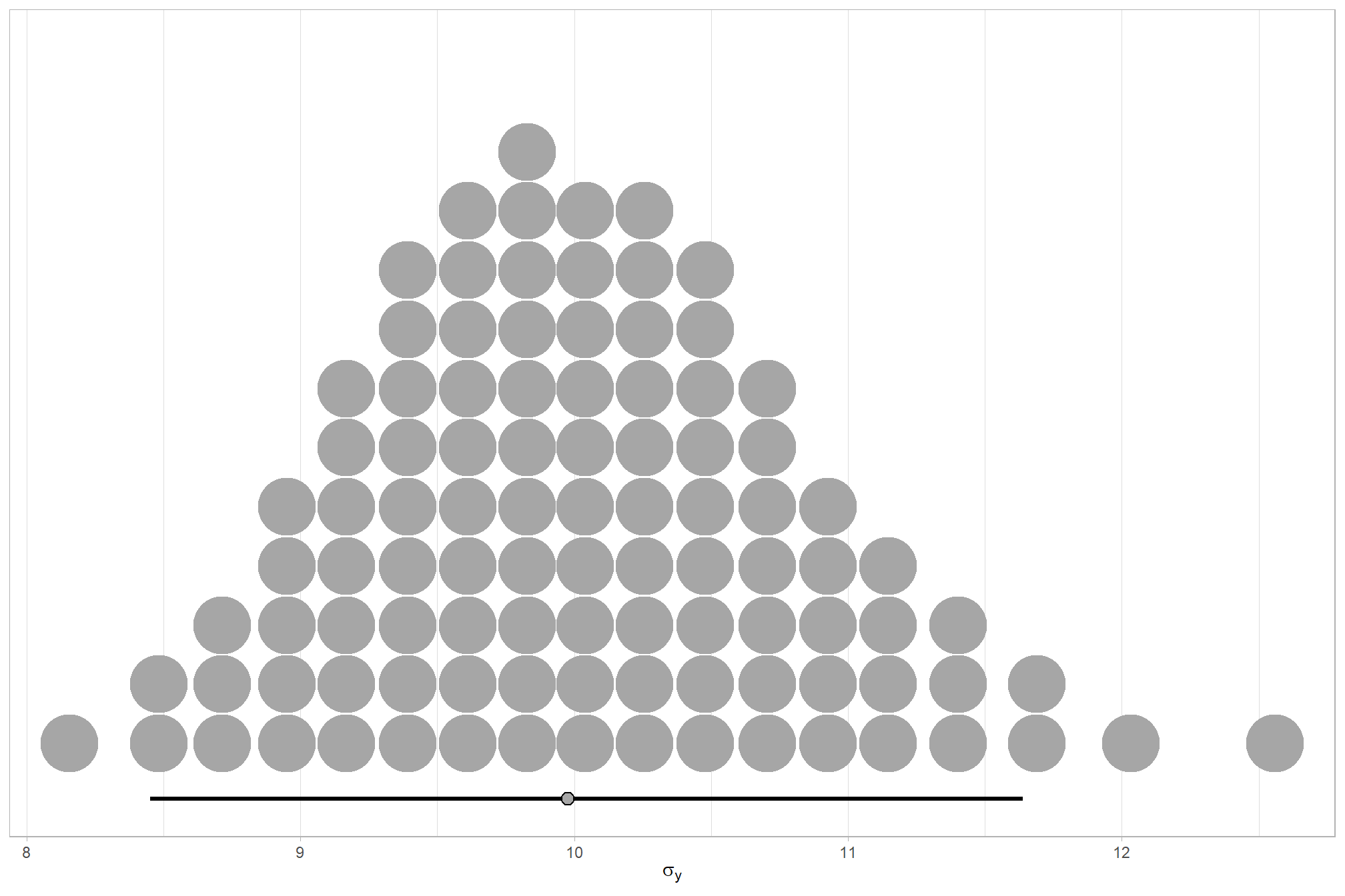
# how is it compared to the first model
dplyr::bind_rows(
    brms::as_draws_df(brms1_mod) %>% tidybayes::median_hdi(sigma) %>% dplyr::mutate(model = "one nominal predictor")
    , brms::as_draws_df(brms2_mod) %>% tidybayes::median_hdi(sigma) %>% dplyr::mutate(model = "two nominal predictor")
  ) %>%
  dplyr::relocate(model) %>%
  kableExtra::kbl(digits = 2, caption = "brms::brm model noise standard deviation comparison") %>%
kableExtra::kable_styling()| model | sigma | .lower | .upper | .width | .point | .interval |
|---|---|---|---|---|---|---|
| one nominal predictor | 12.60 | 10.89 | 14.50 | 0.95 | median | hdi |
| two nominal predictor | 9.98 | 8.45 | 11.64 | 0.95 | median | hdi |
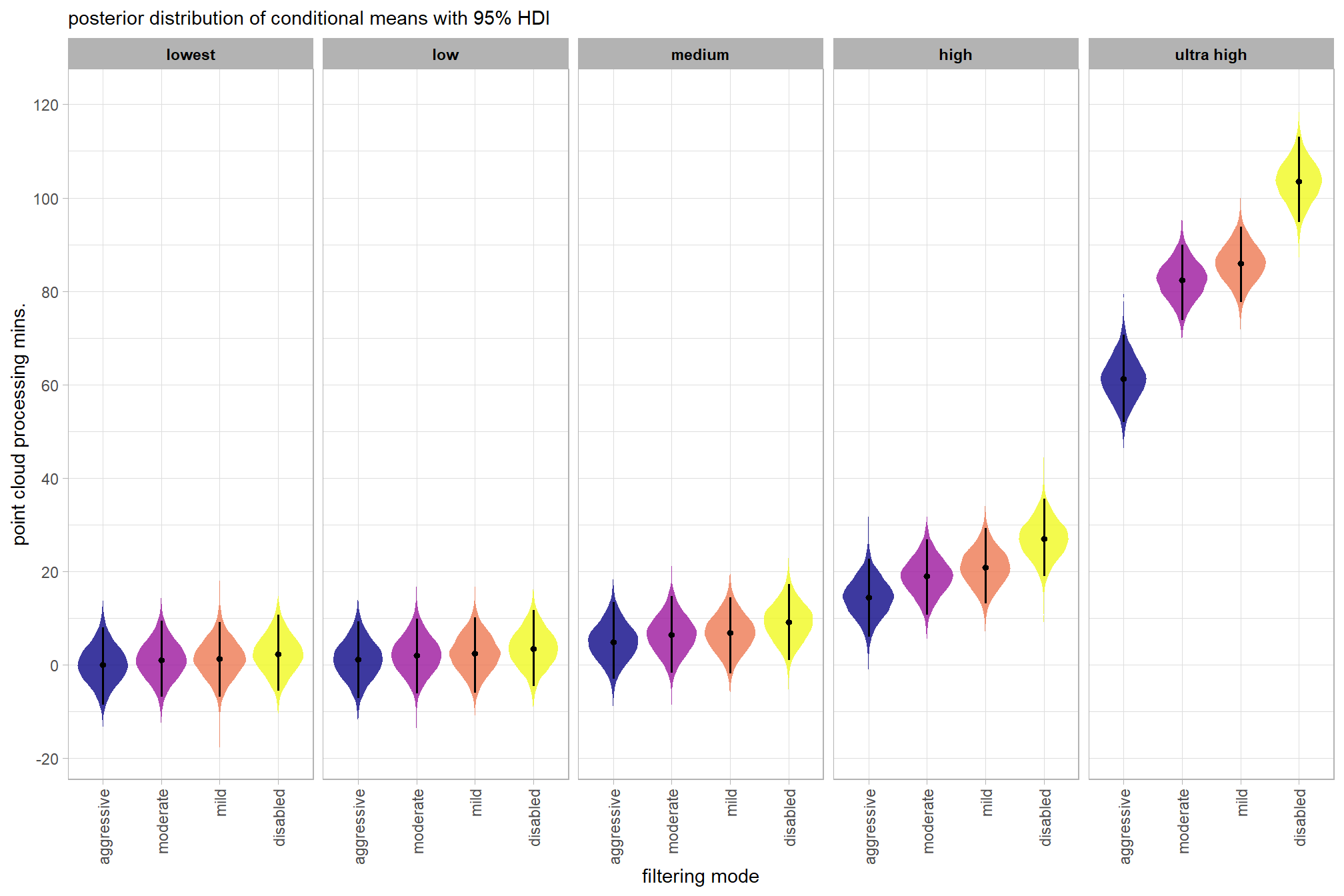
plot the posterior distributions of the conditional means with the median processing time and the 95% highest posterior density interval (HDI)
ptime_data %>%
  dplyr::distinct(depth_maps_generation_quality, depth_maps_generation_filtering_mode) %>%
  tidybayes::add_epred_draws(brms2_mod, allow_new_levels = T) %>%
  dplyr::rename(value = .epred) %>%
  dplyr::mutate(depth_maps_generation_quality = depth_maps_generation_quality %>% forcats::fct_rev()) %>%
  # plot
  ggplot(
    mapping = aes(
      y = value, x = depth_maps_generation_filtering_mode
      , fill = depth_maps_generation_filtering_mode
    )
  ) +
    tidybayes::stat_eye(
      point_interval = median_hdi, .width = .95
      , slab_alpha = 0.8
      , interval_color = "black", linewidth = 1
      , point_color = "black", point_fill = "black", point_size = 1
    ) +
    scale_fill_viridis_d(option = "plasma", drop = F) +
    scale_y_continuous(breaks = scales::extended_breaks(n=10)) +
    facet_grid(cols = vars(depth_maps_generation_quality)) +
    labs(
      x = "filtering mode", y = "point cloud processing mins."
      , subtitle = "posterior distribution of conditional means with 95% HDI"
      , fill = "Filtering Mode"
    ) +
    theme_light() +
    theme(
      legend.position = "none"
      , legend.direction  = "horizontal"
      , axis.text.x = element_text(angle = 90, vjust = 0.5, hjust = 1)
      , strip.text = element_text(color = "black", face = "bold")
) 
    # guides(
    #   fill = guide_legend(reverse = T, override.aes = list(alpha = 1, color = NA, shape = NA, lwd = NA))
    # )
we can also make pairwise comparisons
brms_contrast_temp =
  ptime_data %>%
    dplyr::distinct(depth_maps_generation_quality, depth_maps_generation_filtering_mode) %>%
    tidybayes::add_epred_draws(brms2_mod, allow_new_levels = T) %>%
    dplyr::rename(value = .epred) %>%
    tidybayes::compare_levels(
      value
      , by = depth_maps_generation_quality
      , comparison =
        contrast_list
        # tidybayes::emmeans_comparison("revpairwise")
        #"pairwise"
    ) %>%
    dplyr::rename(contrast = depth_maps_generation_quality)

# separate contrast
brms_contrast_temp = brms_contrast_temp %>%
  dplyr::ungroup() %>%
  tidyr::separate_wider_delim(
    cols = contrast
    , delim = " - "
    , names = paste0(
        "sorter"
        , 1:(max(stringr::str_count(brms_contrast_temp$contrast, "-"))+1)
      )
    , too_few = "align_start"
    , cols_remove = F
  ) %>%
  dplyr::filter(sorter1!=sorter2) %>%
  dplyr::mutate(
    dplyr::across(
      tidyselect::starts_with("sorter")
      , .fns = function(x){factor(
        x, ordered = T
        , levels = levels(ptime_data$depth_maps_generation_quality)
      )}
    )
    , contrast = contrast %>%
      forcats::fct_reorder(
        paste0(as.numeric(sorter1), as.numeric(sorter2)) %>%
        as.numeric()
      )
    , depth_maps_generation_filtering_mode = depth_maps_generation_filtering_mode %>%
      factor(
        levels = levels(ptime_data$depth_maps_generation_filtering_mode)
        , ordered = T
      )
  ) %>%
  # median_hdi summary for coloring
  dplyr::group_by(contrast, depth_maps_generation_filtering_mode) %>%
  dplyr::mutate(
    is_gt_zero = value > 0
    , pct_gt_zero = sum(is_gt_zero)/dplyr::n()
    , sig_level2 = dplyr::case_when(
      pct_gt_zero > 0.99 ~ 0
      , pct_gt_zero > 0.95 ~ 1
      , pct_gt_zero > 0.9 ~ 2
      , pct_gt_zero > 0.8 ~ 3
      , T ~ 4
    ) %>%
    factor(levels = c(0:4), labels = c(">99%","95%","90%","80%","<80%"), ordered = T)
  )

# what?
brms_contrast_temp %>% dplyr::glimpse()
## Rows: 320,000
## Columns: 11
## Groups: contrast, depth_maps_generation_filtering_mode [40]
## $ depth_maps_generation_filtering_mode <ord> aggressive, aggressive, aggressiv…
## $ .chain <int> NA, NA, NA, NA, NA, NA, NA, NA, N…
## $ .iteration <int> NA, NA, NA, NA, NA, NA, NA, NA, N…
## $ .draw <int> 1, 2, 3, 4, 5, 6, 7, 8, 9, 10, 11…
## $ sorter1 <ord> ultra high, ultra high, ultra hig…
## $ sorter2 <ord> high, high, high, high, high, hig…
## $ contrast <fct> ultra high - high, ultra high - h…
## $ value <dbl> 49.69898, 36.26862, 45.16237, 43.…
## $ is_gt_zero <lgl> TRUE, TRUE, TRUE, TRUE, TRUE, TRU…
## $ pct_gt_zero <dbl> 1, 1, 1, 1, 1, 1, 1, 1, 1, 1, 1, …
## $ sig_level2 <ord> >99%, >99%, >99%, >99%, >99%, >99…plot it
# plot it
brms_contrast_temp %>%
  ggplot(
    mapping = aes(
      x = value, y = contrast
      , fill = sig_level2 # pct_gt_zero
      # , fill = depth_maps_generation_filtering_mode
    )
  ) +
    tidybayes::stat_halfeye(
      point_interval = median_hdi, .width = c(0.5,0.95)
      # , slab_fill = "gray22", slab_alpha = 1
      , interval_color = "black", point_color = "black", point_fill = "black"
      , justification = -0.01
    ) +
    geom_vline(xintercept = 0, linetype = "dashed", color = "gray44") +
    scale_fill_viridis_d(
      option = "mako", begin = 0.3
      , drop = F
      # , labels = scales::percent
    ) +
    # scale_fill_viridis_c(
    #   option = "mako", begin = 0.3, direction = -1
    #   , labels = scales::percent
    # ) +
    scale_x_continuous(breaks = scales::extended_breaks(n=8)) +
    facet_grid(cols = vars(depth_maps_generation_filtering_mode)) +
    labs(
      y = "depth map quality"
      , x = "constrast (mins.)"
      , subtitle = "95% & 50% HDI of the posterior distribution of conditional mean group constrasts"
      , fill = "Pr(contrast > 0)"
    ) +
    theme_light() +
    theme(
      legend.position = "top"
      , legend.direction  = "horizontal"
      , strip.text = element_text(color = "black", face = "bold")
    ) +
    guides(
      fill = guide_legend(reverse = T, override.aes = list(alpha = 1, color = NA, shape = NA, lwd = NA))
    )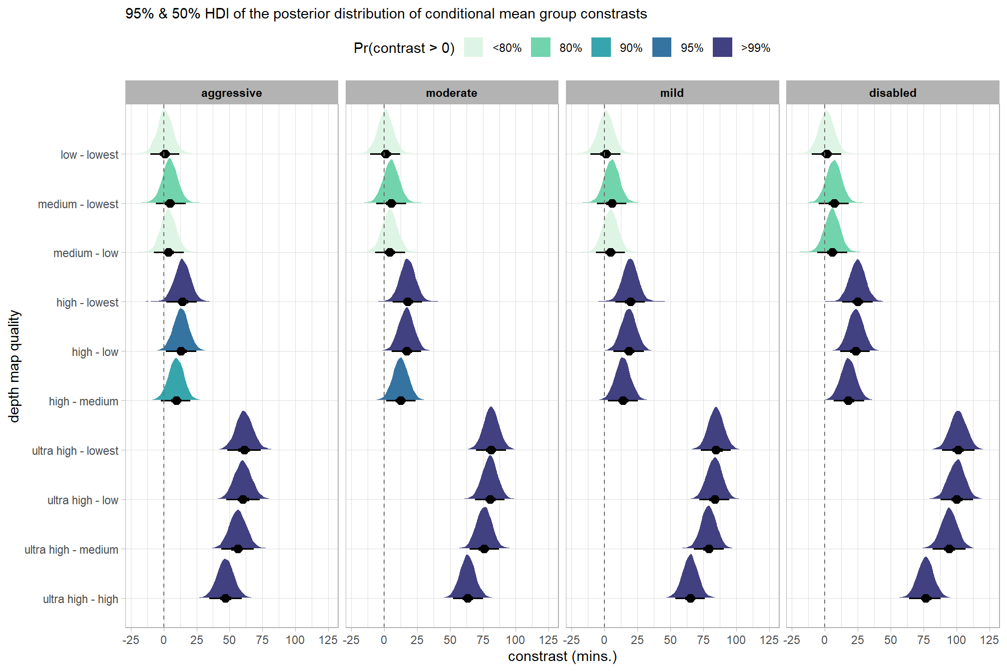
and summarize these contrasts
brms_contrast_temp %>%
  dplyr::group_by(contrast, depth_maps_generation_filtering_mode) %>%
  tidybayes::median_hdi(value) %>%
  dplyr::arrange(contrast, depth_maps_generation_filtering_mode) %>%
  dplyr::select(contrast, depth_maps_generation_filtering_mode, value, .lower, .upper) %>%
  dplyr::rename(difference=value) %>%
kableExtra::kbl(
    digits = 1
    , caption = "brms::brm model: 95% HDI of the posterior distribution of conditional mean group constrasts"
    , col.names = c(
      "quality contrast"
      , "filtering mode"
      , "difference (mins.)"
      , "conf.low", "conf.high"
    )
  ) %>%
  kableExtra::kable_styling() %>%
kableExtra::scroll_box(height = "6in")| quality contrast | filtering mode | difference (mins.) | conf.low | conf.high |
|---|---|---|---|---|
| ultra high - high | aggressive | 46.9 | 34.6 | 59.3 |
| ultra high - high | moderate | 63.4 | 52.3 | 75.0 |
| ultra high - high | mild | 65.2 | 53.7 | 76.4 |
| ultra high - high | disabled | 76.5 | 64.2 | 87.9 |
| ultra high - medium | aggressive | 56.4 | 43.8 | 68.6 |
| ultra high - medium | moderate | 76.1 | 65.0 | 87.4 |
| ultra high - medium | mild | 79.1 | 67.7 | 90.5 |
| ultra high - medium | disabled | 94.4 | 81.8 | 106.7 |
| ultra high - low | aggressive | 60.1 | 47.6 | 73.0 |
| ultra high - low | moderate | 80.4 | 69.0 | 91.5 |
| ultra high - low | mild | 83.7 | 72.2 | 94.7 |
| ultra high - low | disabled | 100.2 | 87.8 | 112.4 |
| ultra high - lowest | aggressive | 61.2 | 48.3 | 73.6 |
| ultra high - lowest | moderate | 81.4 | 69.9 | 92.7 |
| ultra high - lowest | mild | 84.7 | 73.3 | 95.9 |
| ultra high - lowest | disabled | 101.2 | 89.1 | 113.7 |
| high - medium | aggressive | 9.5 | -2.3 | 20.4 |
| high - medium | moderate | 12.6 | 1.6 | 24.1 |
| high - medium | mild | 14.0 | 2.5 | 25.3 |
| high - medium | disabled | 17.9 | 6.6 | 29.7 |
| high - low | aggressive | 13.2 | 1.5 | 24.7 |
| high - low | moderate | 17.0 | 5.8 | 28.1 |
| high - low | mild | 18.5 | 6.9 | 29.8 |
| high - low | disabled | 23.5 | 11.7 | 34.1 |
| high - lowest | aggressive | 14.3 | 2.1 | 25.2 |
| high - lowest | moderate | 17.9 | 6.5 | 29.0 |
| high - lowest | mild | 19.5 | 8.3 | 30.6 |
| high - lowest | disabled | 24.8 | 13.3 | 36.3 |
| medium - low | aggressive | 3.7 | -7.2 | 15.2 |
| medium - low | moderate | 4.4 | -6.7 | 16.1 |
| medium - low | mild | 4.5 | -6.5 | 15.6 |
| medium - low | disabled | 5.6 | -5.7 | 16.9 |
| medium - lowest | aggressive | 4.8 | -6.0 | 16.7 |
| medium - lowest | moderate | 5.4 | -6.1 | 16.6 |
| medium - lowest | mild | 5.6 | -5.7 | 16.7 |
| medium - lowest | disabled | 6.9 | -4.5 | 17.9 |
| low - lowest | aggressive | 1.0 | -10.2 | 12.1 |
| low - lowest | moderate | 1.1 | -10.4 | 12.2 |
| low - lowest | mild | 1.2 | -10.5 | 12.2 |
| low - lowest | disabled | 1.2 | -10.0 | 12.3 |
Kruschke (2015) notes that for the multiple nominal predictors model:
In applications with multiple levels of the factors, it is virtually always the case that we are interested in comparing particular levels with each other…These sorts of comparisons, which involve levels of a single factor and collapse across the other factor(s), are called main effect comparisons or contrasts.(p. 595)
First, let’s collapse across the filtering mode to compare the depth map quality setting effect.
In a hierarchical model structure, we have to make use of the re_formula argument within tidybayes::add_epred_draws
ptime_data %>%
  dplyr::distinct(depth_maps_generation_quality) %>%
  tidybayes::add_epred_draws(
    brms2_mod
    # this part is crucial
    , re_formula = ~ (1 | depth_maps_generation_quality)
  ) %>%
  dplyr::rename(value = .epred) %>%
  # plot
  ggplot(
    mapping = aes(
      x = value, y = depth_maps_generation_quality
      , fill = depth_maps_generation_quality
    )
  ) +
    tidybayes::stat_halfeye(
      point_interval = median_hdi, .width = .95
      , interval_color = "gray66"
      , shape = 21, point_color = "gray66", point_fill = "black"
      , justification = -0.01
    ) +
    scale_fill_viridis_d(option = "inferno", drop = F) +
    scale_x_continuous(breaks = scales::extended_breaks(n=8)) +
    labs(
      y = "depth map quality", x = "point cloud processing mins."
      , subtitle = "posterior distribution of conditional means with 95% HDI"
    ) +
    theme_light() +
    theme(legend.position = "none")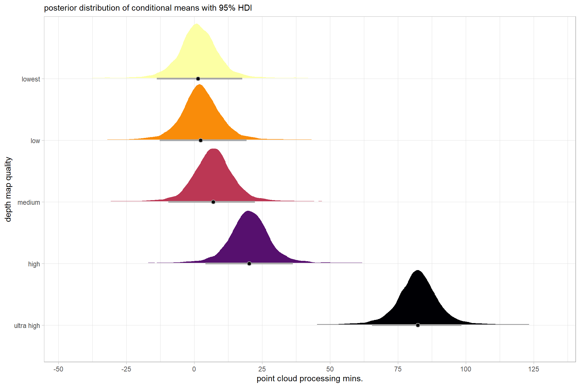
let’s compare these results to the results from our one nominal predictor model above
# let's compare these results to the results from our [one nominal predictor model above](#one_pred_mod)
ptime_data %>%
  dplyr::distinct(depth_maps_generation_quality) %>%
  tidybayes::add_epred_draws(
    brms2_mod
    # this part is crucial
    , re_formula = ~ (1 | depth_maps_generation_quality)
  ) %>%
  dplyr::mutate(value = .epred, src = "two nominal predictor") %>%
  dplyr::bind_rows(
    ptime_data %>%
      dplyr::distinct(depth_maps_generation_quality) %>%
      tidybayes::add_epred_draws(brms1_mod) %>%
      dplyr::mutate(value = .epred, src = "one nominal predictor")
  ) %>%
  ggplot(mapping = aes(y = src, x = value, color = src, group = src)) +
  tidybayes::stat_pointinterval(position = "dodge") +
  facet_grid(rows = vars(depth_maps_generation_quality), switch = "y") +
  scale_y_discrete(NULL, breaks = NULL) +
  scale_color_viridis_d(option = "turbo", begin = 0.2, end = 0.8) +
  labs(
    y = "", x = "point cloud processing mins."
    , color = "model"
  ) +
  theme_light() +
  theme(legend.position = "top", strip.text = element_text(color = "black", face = "bold"))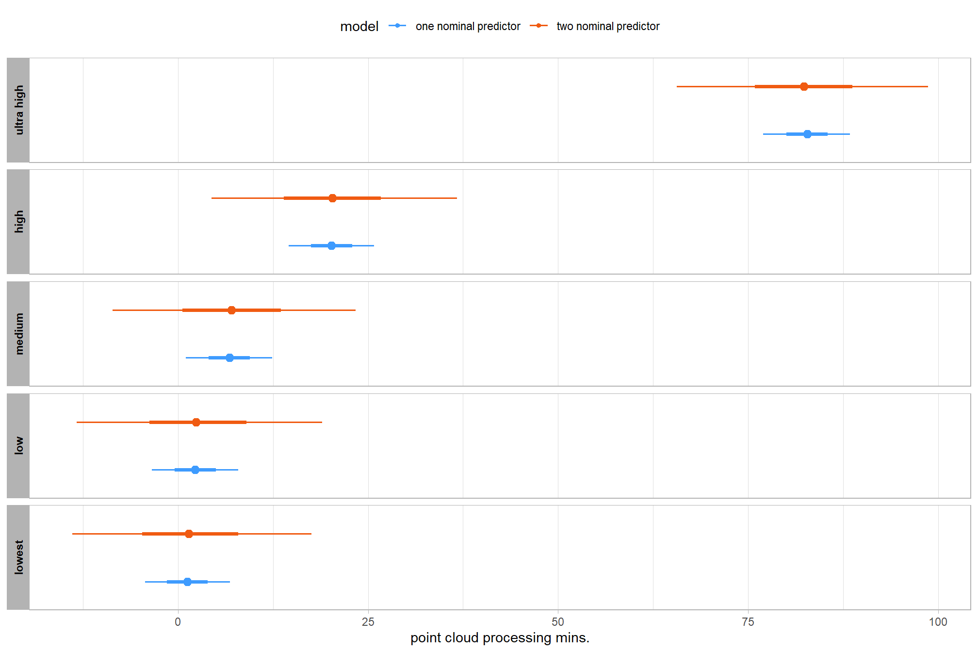
these results are as expected, with Kruschke (2015) noting:
It is important to realize that the estimates of interaction contrasts are typically much more uncertain than the estimates of simple effects or main effects…This large uncertainty of an interaction contrast is caused by the fact that it involves at least four sources of uncertainty (i.e., at least four groups of data), unlike its component simple effects which each involve only half of those sources of uncertainty. In general, interaction contrasts require a lot of data to estimate accurately. (p. 598)
For completeness, let’s also collapse across the depth map quality to compare the filtering mode setting effect.
In a hierarchical model structure, we have to make use of the re_formula argument within tidybayes::add_epred_draws
ptime_data %>%
  dplyr::distinct(depth_maps_generation_filtering_mode) %>%
  tidybayes::add_epred_draws(
    brms2_mod
    # this part is crucial
    , re_formula = ~ (1 | depth_maps_generation_filtering_mode)
  ) %>%
  dplyr::rename(value = .epred) %>%
  # plot
  ggplot(
    mapping = aes(
      x = value, y = depth_maps_generation_filtering_mode
      , fill = depth_maps_generation_filtering_mode
    )
  ) +
    tidybayes::stat_halfeye(
      point_interval = median_hdi, .width = .95
      , interval_color = "gray66"
      , shape = 21, point_color = "gray66", point_fill = "black"
      , justification = -0.01
    ) +
    scale_fill_viridis_d(option = "plasma", drop = F) +
    scale_x_continuous(breaks = scales::extended_breaks(n=8)) +
    labs(
      y = "filtering mode", x = "point cloud processing mins."
      , subtitle = "posterior distribution of conditional means with 95% HDI"
    ) +
    theme_light() +
    theme(legend.position = "none")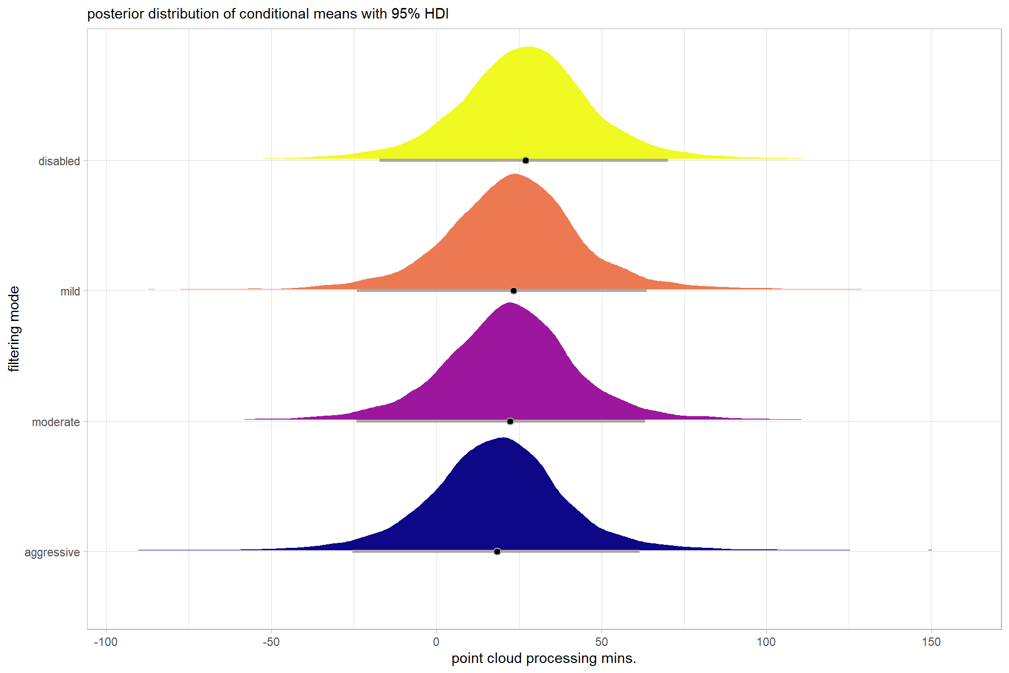
…it looks like the variation in processing time is driven by the depth map quality setting. We can quantify the variation in processing time by comparing the \(\sigma\) posteriors.
# extract the posterior draws
brms::as_draws_df(brms2_mod) %>%
  dplyr::select(c(sigma,tidyselect::starts_with("sd_"))) %>%
  tidyr::pivot_longer(dplyr::everything()) %>%
  # dplyr::group_by(name) %>%
  # tidybayes::median_hdi(value) %>%
  dplyr::mutate(
    name = name %>%
      stringr::str_replace_all("depth_maps_generation_quality", "quality") %>%
      stringr::str_replace_all("depth_maps_generation_filtering_mode", "filtering") %>%
      forcats::fct_reorder(value)
  ) %>%
# plot
  ggplot(aes(x = value, y = name)) +
  tidybayes::stat_dotsinterval(
    point_interval = median_hdi, .width = .95
    , justification = -0.04
    , shape = 21 #, point_size = 3
    , quantiles = 100
  ) +
  labs(x = "", y = "") +
  theme_light()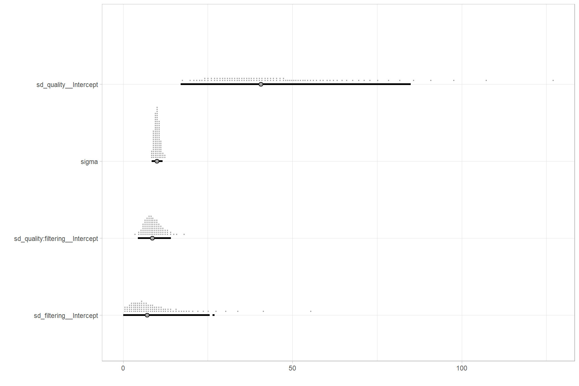
Finally we can perform model selection via information criteria, from section 10 in Kurz’s ebook supplement:
expected log predictive density (
elpd_loo), the estimated effective number of parameters (p_loo), and the Pareto smoothed importance-sampling leave-one-out cross-validation (PSIS-LOO;looic). Each estimate comes with a standard error (i.e.,SE). Like other information criteria, the LOO values aren’t of interest in and of themselves. However, the estimate of one model’s LOO relative to that of another can be of great interest. We generally prefer models with lower information criteria. With thebrms::loo_compare()function, we can compute a formal difference score between two models…Thebrms::loo_compare()output rank orders the models such that the best fitting model appears on top.
brms1_mod = brms::add_criterion(brms1_mod, criterion = c("loo", "waic"))
brms2_mod = brms::add_criterion(brms2_mod, criterion = c("loo", "waic"))
brms::loo_compare(brms1_mod, brms2_mod, criterion = "loo")
## elpd_diff se_diff
## brms2_mod 0.0 0.0
## brms1_mod -16.4 11.94.3 Two Nominal Predictors + site effects
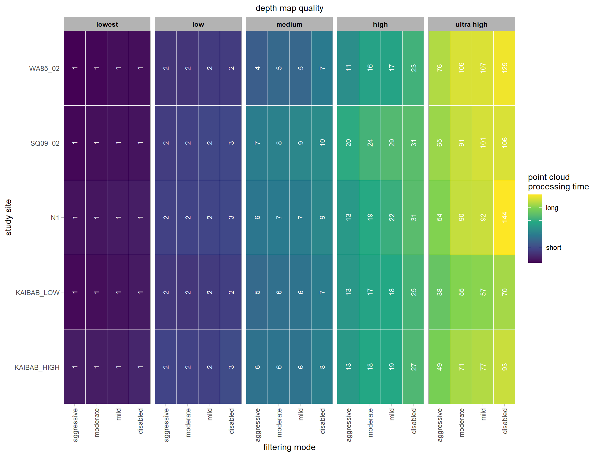
Now, we’ll add the average deflection from the baseline (i.e. the “grand mean”) due to study site (i.e. the “subjects” in our data). The main effect for the study site will be added to our model with the combined influence of the depth map generation quality and the depth map filtering parameters on the point cloud processing time.
In the model we use below, the study site is modeled as a “random effect.” Hobbs et al. (2024) describe a similar model:
It is important to understand that fitting treatment intercepts and slopes as random rather than fixed means that our inference applied to all possible sites suitable for [inclusion in the study]. In contrast, assuming fixed effects of treatment would dramatically reduce the uncertainty about those effects, but would constrain inference to the four sites that we studied. (p. 13)
From this point forward we will only show the Bayesian methodology.
4.3.1 Summary Statistics
Each study site contributes one observation per depth map quality and filtering mode setting. That is, a row in the underlying data is unique by study site, depth map quality, and filtering mode.
identical(
  # base data
  nrow(ptime_data)
  # distinct group
  , ptime_data %>%
    dplyr::distinct(
      study_site
      , depth_maps_generation_quality
      , depth_maps_generation_filtering_mode
    ) %>%
    nrow()
)
## [1] TRUEwe can visualize the data using ggplot2::geom_tile
ptime_data %>%
  dplyr::mutate(
    depth_maps_generation_quality = depth_maps_generation_quality %>% forcats::fct_rev()
  ) %>%
  ggplot(mapping = aes(
    y = study_site
    , x = depth_maps_generation_filtering_mode
    , fill = log(timer_total_time_mins)
  )) +
  geom_tile(color = "white") +
  geom_text(
    mapping = aes(label = round(timer_total_time_mins)), color = "white"
    , size = 3, angle = 90
  ) +
  facet_grid(cols = vars(depth_maps_generation_quality)) +
  scale_x_discrete(expand = c(0, 0)) +
  scale_y_discrete(expand = c(0, 0)) +
  scale_fill_viridis_c(
    option = "viridis"
    , labels = c("", "short","","", "long", "")
  ) +
  labs(
    x = "filtering mode"
    , subtitle = "depth map quality"
    , y = "study site"
    , fill = "point cloud\nprocessing time"
  ) +
  theme_light() +
  theme(
    axis.text.x = element_text(angle = 90, vjust = 0.5, hjust = 1)
    , panel.background = element_blank()
    , panel.grid = element_blank()
    , plot.subtitle = element_text(hjust = 0.5)
    , strip.text = element_text(color = "black", face = "bold")
  )
4.3.2 Bayesian
Kruschke (2015) describes the Hierarchical Bayesian approach to describe groups of metric data with multiple nominal predictors when every subject (“study site” in our research) contributes many measurements to each cell versus situations when each subject only contributes one observation per cell/condition:
When every subject contributes many measurements to every cell, then the model of the situation is a straight-forward extension of the models we have already considered. We merely add “subject” as another nominal predictor in the model, with each individual subject being a level of the predictor. If there is one predictor other than subject, the model becomes
\[ y = \beta_0 + \overrightarrow \beta_1 \overrightarrow x_1 + \overrightarrow \beta_S \overrightarrow x_S + \overrightarrow \beta_{1 \times S} \overrightarrow x_{1 \times S} \]
This is exactly the two-predictor model we have already considered, with the second predictor being subject. When there are two predictors other than subject, the model becomes
\[\begin{align*} y = & \; \beta_0 & \text{baseline} \\ & + \overrightarrow \beta_1 \overrightarrow x_1 + \overrightarrow \beta_2 \overrightarrow x_2 + \overrightarrow \beta_S \overrightarrow x_S & \text{main effects} \\ & + \overrightarrow \beta_{1 \times 2} \overrightarrow x_{1 \times 2} + \overrightarrow \beta_{1 \times S} \overrightarrow x_{1 \times S} + \overrightarrow \beta_{2 \times S} \overrightarrow x_{2 \times S} & \text{two-way interactions} \\ & + \overrightarrow \beta_{1 \times 2 \times S} \overrightarrow x_{1 \times 2 \times S} & \text{three-way interactions} \end{align*}\]
This model includes all the two-way interactions of the factors, plus the three-way interaction. (p. 607)
In situations in which subjects only contribute one observation per condition/cell, we simplify the model to
\[\begin{align*} y = & \; \beta_0 \\ & + \overrightarrow \beta_1 \overrightarrow x_1 + \overrightarrow \beta_2 \overrightarrow x_2 + \overrightarrow \beta_{1 \times 2} \overrightarrow x_{1 \times 2} \\ & + \overrightarrow \beta_S \overrightarrow x_S \end{align*}\]
In other words, we assume a main effect of subject, but no interaction of subject with other predictors. In this model, the subject effect (deflection) is constant across treatments, and the treatment effects (deflections) are constant across subjects. Notice that the model makes no requirement that every subject contributes a datum to every condition. Indeed, the model allows zero or multiple data per subject per condition. Bayesian estimation makes no assumptions or requirements that the design is balanced (i.e., has equal numbers of measurement in each cell). (p. 608)
and see section 20 from Kurz’s ebook supplement
for this model, we’ll define the priors following Kurz:
# from Kurz:
gamma_a_b_from_omega_sigma <- function(mode, sd) {
  if (mode <= 0) stop("mode must be > 0")
  if (sd   <= 0) stop("sd must be > 0")
  rate <- (mode + sqrt(mode^2 + 4 * sd^2)) / (2 * sd^2)
  shape <- 1 + mode * rate
  return(list(shape = shape, rate = rate))
}

mean_y_temp <- mean(ptime_data$timer_total_time_mins)
sd_y_temp   <- sd(ptime_data$timer_total_time_mins)

omega_temp <- sd_y_temp / 2
sigma_temp <- 2 * sd_y_temp

s_r_temp <- gamma_a_b_from_omega_sigma(mode = omega_temp, sd = sigma_temp)

stanvars_temp <-
  brms::stanvar(mean_y_temp,    name = "mean_y") +
  brms::stanvar(sd_y_temp,      name = "sd_y") +
  brms::stanvar(s_r_temp$shape, name = "alpha") +
  brms::stanvar(s_r_temp$rate,  name = "beta")
Now fit the model.
brms3_mod = brms::brm(
formula = timer_total_time_mins ~ 1 +
(1 | depth_maps_generation_quality) +
(1 | depth_maps_generation_filtering_mode) +
(1 | depth_maps_generation_quality:depth_maps_generation_filtering_mode) +
(1 | study_site)
, data = ptime_data
, family = brms::brmsfamily(family = "gaussian")
, iter = 4000, warmup = 2000, chains = 4
, cores = round(parallel::detectCores()/2)
, prior = c(
brms::prior(normal(mean_y, sd_y * 5), class = "Intercept")
, brms::prior(gamma(alpha, beta), class = "sd")
, brms::prior(cauchy(0, sd_y), class = "sigma")
)
, stanvars = stanvars_temp
, file = paste0(rootdir, "/fits/brms3_mod")
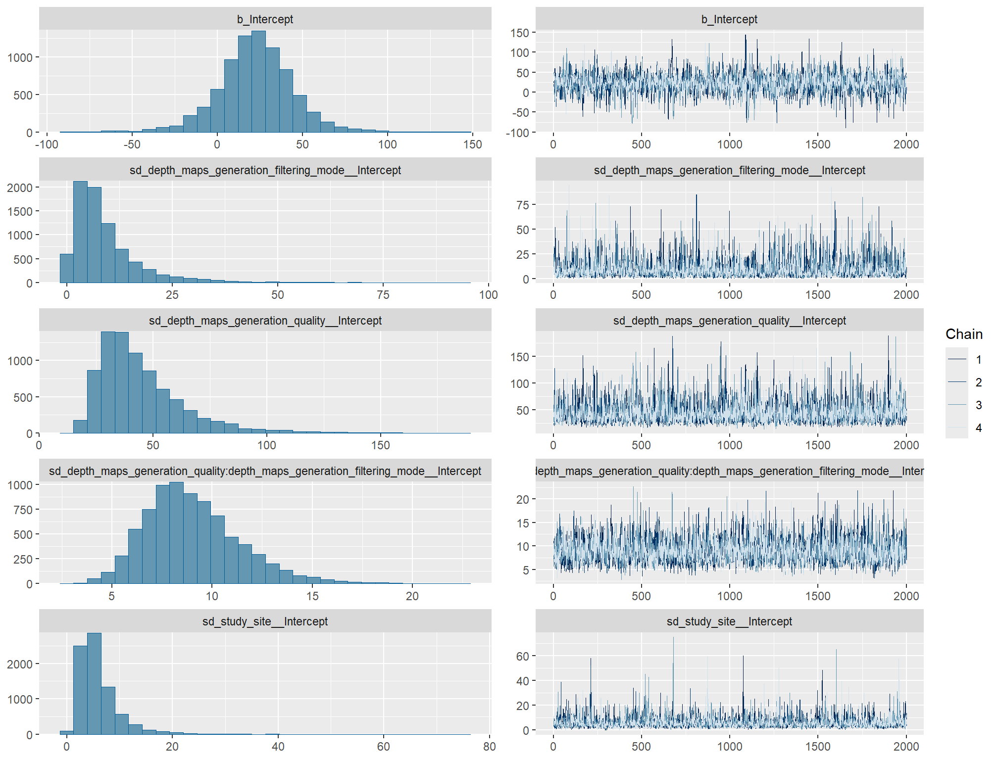
)check the trace plots for problems with convergence of the Markov chains
check the prior distributions
| prior | class | coef | group | resp | dpar | nlpar | lb | ub | source |
|---|---|---|---|---|---|---|---|---|---|
| normal(mean_y, sd_y * 5) | Intercept | user | |||||||
| gamma(alpha, beta) | sd | 0 | user | ||||||
| sd | depth_maps_generation_filtering_mode | default | |||||||
| sd | Intercept | depth_maps_generation_filtering_mode | default | ||||||
| sd | depth_maps_generation_quality | default | |||||||
| sd | Intercept | depth_maps_generation_quality | default | ||||||
| sd | depth_maps_generation_quality:depth_maps_generation_filtering_mode | default | |||||||
| sd | Intercept | depth_maps_generation_quality:depth_maps_generation_filtering_mode | default | ||||||
| sd | study_site | default | |||||||
| sd | Intercept | study_site | default | ||||||
| cauchy(0, sd_y) | sigma | 0 | user |
The brms::brm model summary
brms3_mod %>%
  brms::posterior_summary() %>%
  as.data.frame() %>%
  tibble::rownames_to_column(var = "parameter") %>%
  dplyr::rename_with(tolower) %>%
  dplyr::filter(
    stringr::str_starts(parameter, "b_")
    | stringr::str_starts(parameter, "r_")
    | stringr::str_starts(parameter, "sd_")
    | parameter == "sigma"
  ) %>%
  dplyr::mutate(
    parameter = parameter %>%
      stringr::str_replace_all("depth_maps_generation_quality", "quality") %>%
      stringr::str_replace_all("depth_maps_generation_filtering_mode", "filtering")
  ) %>%
  kableExtra::kbl(digits = 2, caption = "Bayesian two nominal predictors + study site effects for point cloud processing time") %>%
  kableExtra::kable_styling() %>%
kableExtra::scroll_box(height = "6in")| parameter | estimate | est.error | q2.5 | q97.5 |
|---|---|---|---|---|
| b_Intercept | 22.32 | 22.53 | -23.77 | 67.69 |
| sd_filtering__Intercept | 9.26 | 8.88 | 0.71 | 33.16 |
| sd_quality__Intercept | 44.93 | 19.97 | 21.31 | 97.68 |
| sd_quality:filtering__Intercept | 9.04 | 2.42 | 5.22 | 14.65 |
| sd_study_site__Intercept | 6.09 | 4.47 | 1.67 | 17.50 |
| sigma | 9.32 | 0.77 | 7.95 | 11.01 |
| r_filtering[aggressive,Intercept] | -4.29 | 6.86 | -19.55 | 7.94 |
| r_filtering[moderate,Intercept] | -0.30 | 6.55 | -13.86 | 13.28 |
| r_filtering[mild,Intercept] | 0.55 | 6.56 | -12.14 | 14.80 |
| r_filtering[disabled,Intercept] | 4.39 | 6.88 | -6.86 | 19.95 |
| r_quality[ultra.high,Intercept] | 59.88 | 21.87 | 16.82 | 105.55 |
| r_quality[high,Intercept] | -2.00 | 21.92 | -45.98 | 43.30 |
| r_quality[medium,Intercept] | -15.36 | 21.92 | -59.34 | 28.81 |
| r_quality[low,Intercept] | -19.83 | 22.09 | -64.57 | 25.85 |
| r_quality[lowest,Intercept] | -20.87 | 22.01 | -65.27 | 23.19 |
| r_quality:filtering[high_aggressive,Intercept] | -1.69 | 6.38 | -14.52 | 10.70 |
| r_quality:filtering[high_disabled,Intercept] | 2.33 | 6.35 | -10.03 | 15.09 |
| r_quality:filtering[high_mild,Intercept] | -0.08 | 6.19 | -12.18 | 12.18 |
| r_quality:filtering[high_moderate,Intercept] | -1.09 | 6.07 | -13.09 | 11.02 |
| r_quality:filtering[low_aggressive,Intercept] | 3.06 | 6.43 | -9.41 | 15.83 |
| r_quality:filtering[low_disabled,Intercept] | -3.52 | 6.37 | -16.45 | 8.99 |
| r_quality:filtering[low_mild,Intercept] | -0.69 | 6.05 | -12.66 | 11.57 |
| r_quality:filtering[low_moderate,Intercept] | -0.09 | 6.23 | -12.69 | 12.34 |
| r_quality:filtering[lowest_aggressive,Intercept] | 3.03 | 6.48 | -9.99 | 15.88 |
| r_quality:filtering[lowest_disabled,Intercept] | -3.74 | 6.44 | -16.55 | 8.76 |
| r_quality:filtering[lowest_mild,Intercept] | -0.74 | 6.34 | -13.51 | 11.56 |
| r_quality:filtering[lowest_moderate,Intercept] | -0.11 | 6.30 | -12.83 | 12.61 |
| r_quality:filtering[medium_aggressive,Intercept] | 2.39 | 6.48 | -10.44 | 15.13 |
| r_quality:filtering[medium_disabled,Intercept] | -2.33 | 6.49 | -15.04 | 10.73 |
| r_quality:filtering[medium_mild,Intercept] | -0.72 | 6.26 | -13.26 | 11.59 |
| r_quality:filtering[medium_moderate,Intercept] | -0.27 | 6.28 | -12.89 | 12.39 |
| r_quality:filtering[ultra.high_aggressive,Intercept] | -17.33 | 6.73 | -30.77 | -4.71 |
| r_quality:filtering[ultra.high_disabled,Intercept] | 17.58 | 6.98 | 4.84 | 32.18 |
| r_quality:filtering[ultra.high_mild,Intercept] | 3.41 | 6.41 | -8.76 | 16.85 |
| r_quality:filtering[ultra.high_moderate,Intercept] | 0.44 | 6.24 | -11.81 | 13.09 |
| r_study_site[KAIBAB_HIGH,Intercept] | -1.93 | 3.67 | -9.41 | 5.02 |
| r_study_site[KAIBAB_LOW,Intercept] | -5.14 | 3.82 | -13.38 | 1.60 |
| r_study_site[N1,Intercept] | 2.18 | 3.76 | -4.89 | 10.04 |
| r_study_site[SQ09_02,Intercept] | 2.35 | 3.68 | -4.57 | 10.03 |
| r_study_site[WA85_02,Intercept] | 2.46 | 3.72 | -4.60 | 10.47 |
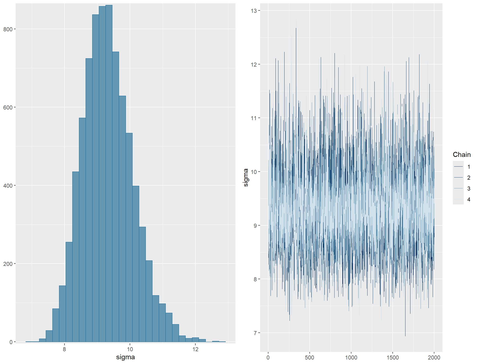
We can look at the model noise standard deviation \(\sigma_y\)
# extract the posterior draws
brms::as_draws_df(brms3_mod) %>%
# plot
  ggplot(aes(x = sigma, y = 0)) +
  tidybayes::stat_dotsinterval(
    point_interval = median_hdi, .width = .95
    , justification = -0.04
    , shape = 21, point_size = 3
    , quantiles = 100
  ) +
  scale_y_continuous(NULL, breaks = NULL) +
  xlab(latex2exp::TeX("$\\sigma_y$")) +
  theme_light()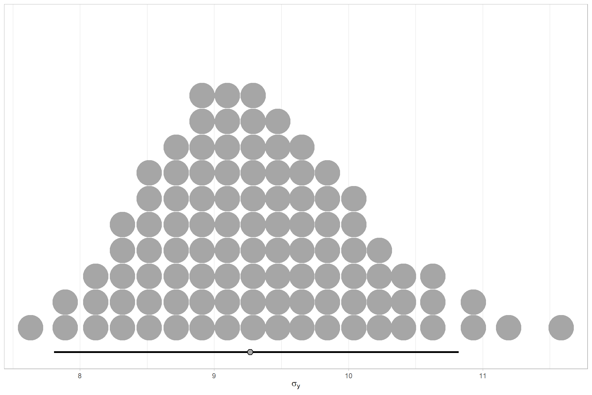
# how is it compared to our other models?
dplyr::bind_rows(
    brms::as_draws_df(brms1_mod) %>% tidybayes::median_hdi(sigma) %>% dplyr::mutate(model = "one nominal predictor")
    , brms::as_draws_df(brms2_mod) %>% tidybayes::median_hdi(sigma) %>% dplyr::mutate(model = "two nominal predictor")
    , brms::as_draws_df(brms3_mod) %>% tidybayes::median_hdi(sigma) %>% dplyr::mutate(model = "two nominal predictor + site effect")
  ) %>%
  dplyr::relocate(model) %>%
  kableExtra::kbl(digits = 2, caption = "brms::brm model noise standard deviation comparison") %>%
kableExtra::kable_styling()| model | sigma | .lower | .upper | .width | .point | .interval |
|---|---|---|---|---|---|---|
| one nominal predictor | 12.60 | 10.89 | 14.50 | 0.95 | median | hdi |
| two nominal predictor | 9.98 | 8.45 | 11.64 | 0.95 | median | hdi |
| two nominal predictor + site effect | 9.27 | 7.81 | 10.82 | 0.95 | median | hdi |
plot the posterior distributions of the conditional means with the median processing time and the 95% highest posterior density interval (HDI)
Note that how within tidybayes::add_epred_draws, we used the re_formula argument to average over the random effects of study_site (i.e., we left (1 | study_site) out of the formula). For this model we have to collapse across the study site effects to compare the depth map quality and filtering mode setting effects.
ptime_data %>%
  dplyr::distinct(depth_maps_generation_quality, depth_maps_generation_filtering_mode) %>%
  tidybayes::add_epred_draws(
    brms3_mod, allow_new_levels = T
    # this part is crucial
    , re_formula = ~ (1 | depth_maps_generation_quality) +
      (1 | depth_maps_generation_filtering_mode) +
      (1 | depth_maps_generation_quality:depth_maps_generation_filtering_mode)
  ) %>%
  dplyr::rename(value = .epred) %>%
  dplyr::mutate(depth_maps_generation_quality = depth_maps_generation_quality %>% forcats::fct_rev()) %>%
  # plot
  ggplot(
    mapping = aes(
      y = value, x = depth_maps_generation_filtering_mode
      , fill = depth_maps_generation_filtering_mode
    )
  ) +
    tidybayes::stat_eye(
      point_interval = median_hdi, .width = .95
      , slab_alpha = 0.8
      , interval_color = "black", linewidth = 1
      , point_color = "black", point_fill = "black", point_size = 1
    ) +
    scale_fill_viridis_d(option = "plasma", drop = F) +
    scale_y_continuous(breaks = scales::extended_breaks(n=10)) +
    facet_grid(cols = vars(depth_maps_generation_quality)) +
    labs(
      x = "filtering mode", y = "point cloud processing mins."
      , subtitle = "posterior distribution of conditional means with 95% HDI"
      , fill = "Filtering Mode"
    ) +
    theme_light() +
    theme(
      legend.position = "none"
      , legend.direction  = "horizontal"
      , axis.text.x = element_text(angle = 90, vjust = 0.5, hjust = 1)
      , strip.text = element_text(color = "black", face = "bold")
) 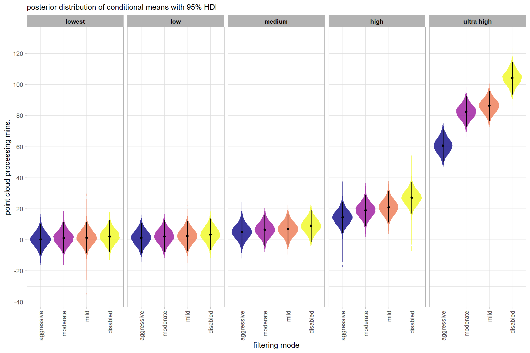
    # guides(
    #   fill = guide_legend(reverse = T, override.aes = list(alpha = 1, color = NA, shape = NA, lwd = NA))
    # )
we can also make pairwise comparisons so long as we continue using tidybayes::add_epred_draws with the re_formula argument
brms_contrast_temp =
  ptime_data %>%
    dplyr::distinct(depth_maps_generation_quality, depth_maps_generation_filtering_mode) %>%
    tidybayes::add_epred_draws(
      brms3_mod, allow_new_levels = T
      # this part is crucial
      , re_formula = ~ (1 | depth_maps_generation_quality) +
        (1 | depth_maps_generation_filtering_mode) +
        (1 | depth_maps_generation_quality:depth_maps_generation_filtering_mode)
    ) %>%
    dplyr::rename(value = .epred) %>%
    tidybayes::compare_levels(
      value
      , by = depth_maps_generation_quality
      , comparison =
        contrast_list
        # tidybayes::emmeans_comparison("revpairwise")
        #"pairwise"
    ) %>%
    dplyr::rename(contrast = depth_maps_generation_quality)

# separate contrast
brms_contrast_temp = brms_contrast_temp %>%
  dplyr::ungroup() %>%
  tidyr::separate_wider_delim(
    cols = contrast
    , delim = " - "
    , names = paste0(
        "sorter"
        , 1:(max(stringr::str_count(brms_contrast_temp$contrast, "-"))+1)
      )
    , too_few = "align_start"
    , cols_remove = F
  ) %>%
  dplyr::filter(sorter1!=sorter2) %>%
  dplyr::mutate(
    dplyr::across(
      tidyselect::starts_with("sorter")
      , .fns = function(x){factor(
        x, ordered = T
        , levels = levels(ptime_data$depth_maps_generation_quality)
      )}
    )
    , contrast = contrast %>%
      forcats::fct_reorder(
        paste0(as.numeric(sorter1), as.numeric(sorter2)) %>%
        as.numeric()
      )
    , depth_maps_generation_filtering_mode = depth_maps_generation_filtering_mode %>%
      factor(
        levels = levels(ptime_data$depth_maps_generation_filtering_mode)
        , ordered = T
      )
  ) %>%
  # median_hdi summary for coloring
  dplyr::group_by(contrast, depth_maps_generation_filtering_mode) %>%
  dplyr::mutate(
    is_gt_zero = value > 0
    , pct_gt_zero = sum(is_gt_zero)/dplyr::n()
    , sig_level2 = dplyr::case_when(
      pct_gt_zero > 0.99 ~ 0
      , pct_gt_zero > 0.95 ~ 1
      , pct_gt_zero > 0.9 ~ 2
      , pct_gt_zero > 0.8 ~ 3
      , T ~ 4
    ) %>%
    factor(levels = c(0:4), labels = c(">99%","95%","90%","80%","<80%"), ordered = T)
  )

# what?
brms_contrast_temp %>% dplyr::glimpse()
## Rows: 320,000
## Columns: 11
## Groups: contrast, depth_maps_generation_filtering_mode [40]
## $ depth_maps_generation_filtering_mode <ord> aggressive, aggressive, aggressiv…
## $ .chain <int> NA, NA, NA, NA, NA, NA, NA, NA, N…
## $ .iteration <int> NA, NA, NA, NA, NA, NA, NA, NA, N…
## $ .draw <int> 1, 2, 3, 4, 5, 6, 7, 8, 9, 10, 11…
## $ sorter1 <ord> ultra high, ultra high, ultra hig…
## $ sorter2 <ord> high, high, high, high, high, hig…
## $ contrast <fct> ultra high - high, ultra high - h…
## $ value <dbl> 56.16488, 38.73338, 50.98472, 48.…
## $ is_gt_zero <lgl> TRUE, TRUE, TRUE, TRUE, TRUE, TRU…
## $ pct_gt_zero <dbl> 1, 1, 1, 1, 1, 1, 1, 1, 1, 1, 1, …
## $ sig_level2 <ord> >99%, >99%, >99%, >99%, >99%, >99…plot it
# plot it
brms_contrast_temp %>%
  ggplot(
    mapping = aes(
      x = value, y = contrast
      , fill = sig_level2 # pct_gt_zero
      # , fill = depth_maps_generation_filtering_mode
    )
  ) +
    tidybayes::stat_halfeye(
      point_interval = median_hdi, .width = c(0.5,0.95)
      # , slab_fill = "gray22", slab_alpha = 1
      , interval_color = "black", point_color = "black", point_fill = "black"
      , justification = -0.01
    ) +
    geom_vline(xintercept = 0, linetype = "dashed", color = "gray44") +
    scale_fill_viridis_d(
      option = "mako", begin = 0.3
      , drop = F
      # , labels = scales::percent
    ) +
    # scale_fill_viridis_c(
    #   option = "mako", begin = 0.3, direction = -1
    #   , labels = scales::percent
    # ) +
    scale_x_continuous(breaks = scales::extended_breaks(n=8)) +
    facet_grid(cols = vars(depth_maps_generation_filtering_mode)) +
    labs(
      y = "depth map quality"
      , x = "constrast (mins.)"
      , subtitle = "95% & 50% HDI of the posterior distribution of conditional mean group constrasts"
      , fill = "Pr(contrast > 0)"
    ) +
    theme_light() +
    theme(
      legend.position = "top"
      , legend.direction  = "horizontal"
      , strip.text = element_text(color = "black", face = "bold")
    ) +
    guides(
      fill = guide_legend(reverse = T, override.aes = list(alpha = 1, color = NA, shape = NA, lwd = NA))
    )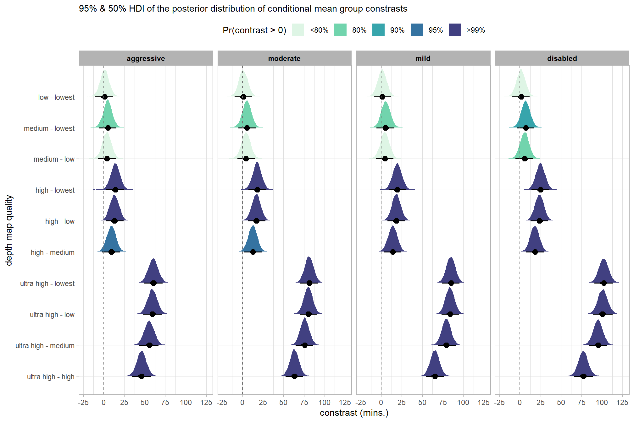
and summarize these contrasts
brms_contrast_temp %>%
  dplyr::group_by(contrast, depth_maps_generation_filtering_mode) %>%
  tidybayes::median_hdi(value) %>%
  dplyr::arrange(contrast, depth_maps_generation_filtering_mode) %>%
  dplyr::select(contrast, depth_maps_generation_filtering_mode, value, .lower, .upper) %>%
  dplyr::rename(difference=value) %>%
kableExtra::kbl(
    digits = 1
    , caption = "brms::brm model: 95% HDI of the posterior distribution of conditional mean group constrasts"
    , col.names = c(
      "quality contrast"
      , "filtering mode"
      , "difference (mins.)"
      , "conf.low", "conf.high"
    )
  ) %>%
  kableExtra::kable_styling() %>%
kableExtra::scroll_box(height = "6in")| quality contrast | filtering mode | difference (mins.) | conf.low | conf.high |
|---|---|---|---|---|
| ultra high - high | aggressive | 46.3 | 34.6 | 57.6 |
| ultra high - high | moderate | 63.4 | 52.6 | 74.0 |
| ultra high - high | mild | 65.4 | 54.5 | 76.2 |
| ultra high - high | disabled | 77.1 | 66.1 | 88.9 |
| ultra high - medium | aggressive | 55.5 | 43.5 | 66.6 |
| ultra high - medium | moderate | 75.9 | 64.8 | 86.0 |
| ultra high - medium | mild | 79.4 | 69.1 | 90.6 |
| ultra high - medium | disabled | 95.2 | 83.8 | 106.6 |
| ultra high - low | aggressive | 59.3 | 48.0 | 71.1 |
| ultra high - low | moderate | 80.2 | 69.8 | 90.8 |
| ultra high - low | mild | 83.8 | 73.4 | 94.5 |
| ultra high - low | disabled | 100.9 | 89.2 | 112.8 |
| ultra high - lowest | aggressive | 60.4 | 48.6 | 72.0 |
| ultra high - lowest | moderate | 81.3 | 70.5 | 92.0 |
| ultra high - lowest | mild | 84.9 | 73.9 | 95.4 |
| ultra high - lowest | disabled | 102.0 | 90.5 | 113.9 |
| high - medium | aggressive | 9.3 | -1.8 | 19.9 |
| high - medium | moderate | 12.6 | 1.9 | 23.4 |
| high - medium | mild | 14.1 | 2.9 | 24.3 |
| high - medium | disabled | 18.0 | 7.5 | 28.9 |
| high - low | aggressive | 13.1 | 3.0 | 24.3 |
| high - low | moderate | 16.9 | 6.5 | 28.1 |
| high - low | mild | 18.4 | 7.7 | 29.1 |
| high - low | disabled | 23.7 | 13.0 | 34.5 |
| high - lowest | aggressive | 14.2 | 3.3 | 24.7 |
| high - lowest | moderate | 17.9 | 7.3 | 28.6 |
| high - lowest | mild | 19.5 | 9.0 | 30.6 |
| high - lowest | disabled | 25.0 | 14.2 | 35.9 |
| medium - low | aggressive | 3.9 | -6.8 | 14.6 |
| medium - low | moderate | 4.3 | -6.3 | 15.4 |
| medium - low | mild | 4.4 | -6.2 | 15.0 |
| medium - low | disabled | 5.6 | -5.6 | 15.7 |
| medium - lowest | aggressive | 4.9 | -5.9 | 15.4 |
| medium - lowest | moderate | 5.4 | -4.9 | 16.6 |
| medium - lowest | mild | 5.5 | -5.7 | 15.9 |
| medium - lowest | disabled | 6.9 | -3.8 | 17.5 |
| low - lowest | aggressive | 1.1 | -10.2 | 11.1 |
| low - lowest | moderate | 1.0 | -9.5 | 12.1 |
| low - lowest | mild | 1.1 | -9.1 | 12.1 |
| low - lowest | disabled | 1.3 | -9.4 | 11.8 |
let’s collapse across the filtering mode and study site to compare the depth map quality setting effect.
In a hierarchical model structure, we have to make use of the re_formula argument within tidybayes::add_epred_draws
ptime_data %>%
  dplyr::distinct(depth_maps_generation_quality) %>%
  tidybayes::add_epred_draws(
    brms3_mod
    # this part is crucial
    , re_formula = ~ (1 | depth_maps_generation_quality)
  ) %>%
  dplyr::rename(value = .epred) %>%
  # plot
  ggplot(
    mapping = aes(
      x = value, y = depth_maps_generation_quality
      , fill = depth_maps_generation_quality
    )
  ) +
    tidybayes::stat_halfeye(
      point_interval = median_hdi, .width = .95
      , interval_color = "gray66"
      , shape = 21, point_color = "gray66", point_fill = "black"
      , justification = -0.01
    ) +
    scale_fill_viridis_d(option = "inferno", drop = F) +
    scale_x_continuous(breaks = scales::extended_breaks(n=8)) +
    labs(
      y = "depth map quality", x = "point cloud processing mins."
      , subtitle = "posterior distribution of conditional means with 95% HDI"
    ) +
    theme_light() +
    theme(legend.position = "none")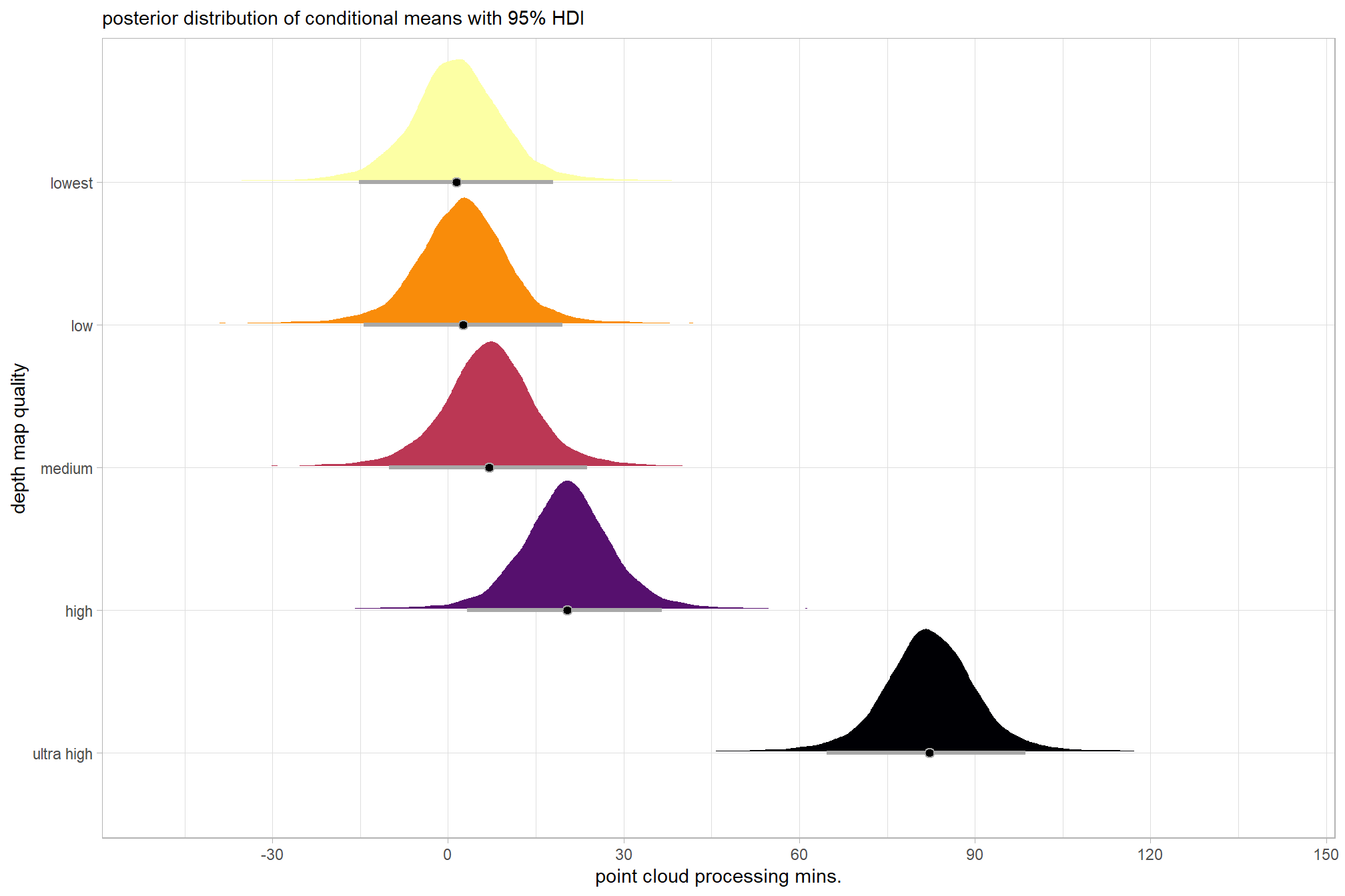
let’s compare these results to the results from our one nominal predictor model above and two nominal predictor model without site effects above
ptime_data %>%
  dplyr::distinct(depth_maps_generation_quality) %>%
  tidybayes::add_epred_draws(
    brms3_mod
    # this part is crucial
    , re_formula = ~ (1 | depth_maps_generation_quality)
  ) %>%
  dplyr::mutate(value = .epred, src = "site+two nominal predictor") %>%
  dplyr::bind_rows(
    ptime_data %>%
      dplyr::distinct(depth_maps_generation_quality) %>%
      tidybayes::add_epred_draws(
        brms2_mod
        # this part is crucial
        , re_formula = ~ (1 | depth_maps_generation_quality)
      ) %>%
      dplyr::mutate(value = .epred, src = "two nominal predictor")
    , ptime_data %>%
      dplyr::distinct(depth_maps_generation_quality) %>%
      tidybayes::add_epred_draws(brms1_mod) %>%
      dplyr::mutate(value = .epred, src = "one nominal predictor")
  ) %>%
  ggplot(mapping = aes(y = src, x = value, color = src, group = src)) +
  tidybayes::stat_pointinterval(position = "dodge") +
  facet_grid(rows = vars(depth_maps_generation_quality), switch = "y") +
  scale_y_discrete(NULL, breaks = NULL) +
  # scale_color_viridis_d(option = "turbo", begin = 0.2, end = 0.8) +
  scale_color_manual(values = viridis::turbo(n = 4, begin = 0.2, end = 0.8)[c(1,3:4)]) +
  labs(
    y = "", x = "point cloud processing mins."
    , color = "model"
  ) +
  theme_light() +
  theme(legend.position = "top", strip.text = element_text(color = "black", face = "bold"))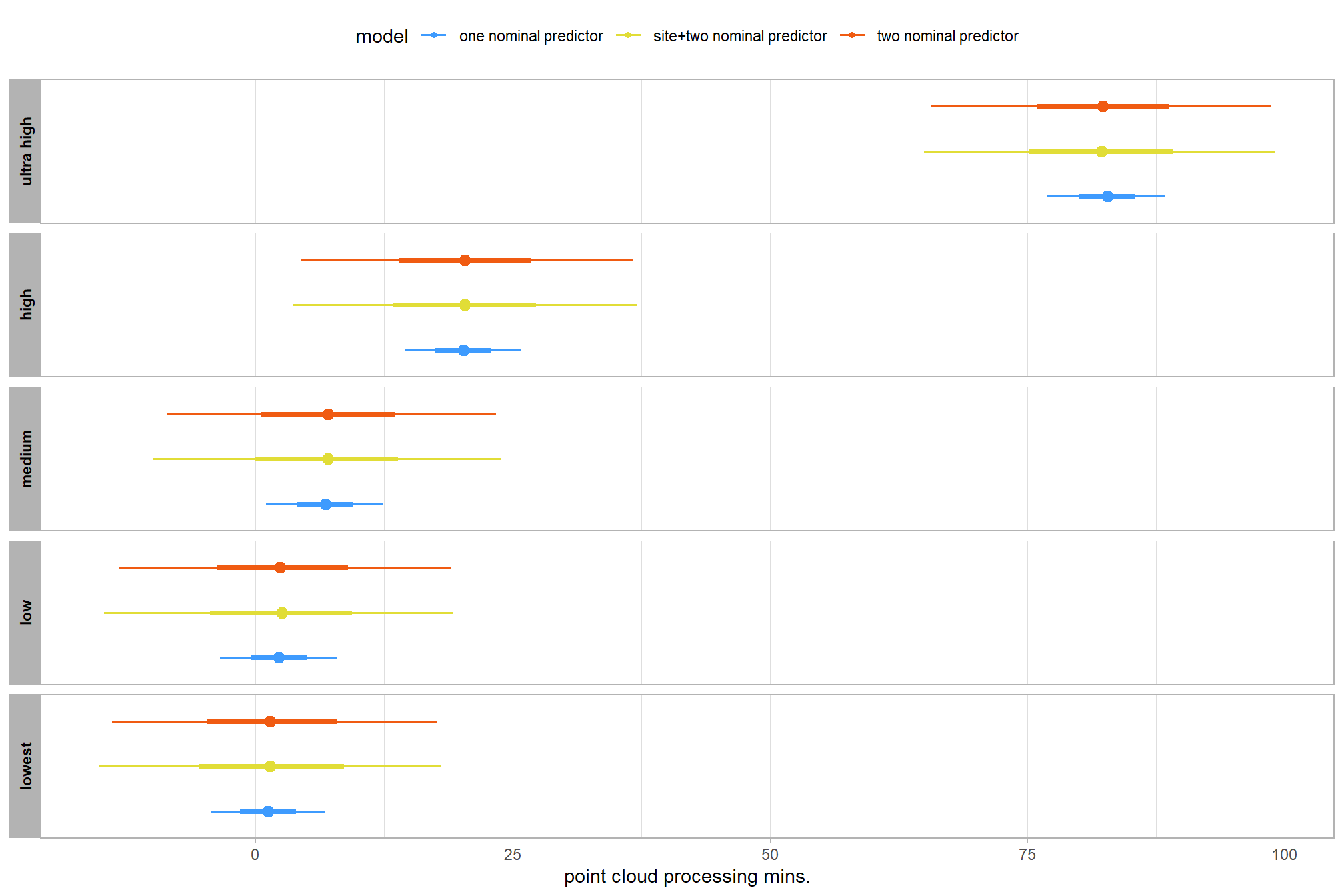
For completeness, let’s also collapse across the depth map quality to compare the filtering mode setting effect.
In a hierarchical model structure, we have to make use of the re_formula argument within tidybayes::add_epred_draws
ptime_data %>%
  dplyr::distinct(depth_maps_generation_filtering_mode) %>%
  tidybayes::add_epred_draws(
    brms3_mod
    # this part is crucial
    , re_formula = ~ (1 | depth_maps_generation_filtering_mode)
  ) %>%
  dplyr::rename(value = .epred) %>%
  # plot
  ggplot(
    mapping = aes(
      x = value, y = depth_maps_generation_filtering_mode
      , fill = depth_maps_generation_filtering_mode
    )
  ) +
    tidybayes::stat_halfeye(
      point_interval = median_hdi, .width = .95
      , interval_color = "gray66"
      , shape = 21, point_color = "gray66", point_fill = "black"
      , justification = -0.01
    ) +
    scale_fill_viridis_d(option = "plasma", drop = F) +
    scale_x_continuous(breaks = scales::extended_breaks(n=8)) +
    labs(
      y = "filtering mode", x = "point cloud processing mins."
      , subtitle = "posterior distribution of conditional means with 95% HDI"
    ) +
    theme_light() +
    theme(legend.position = "none")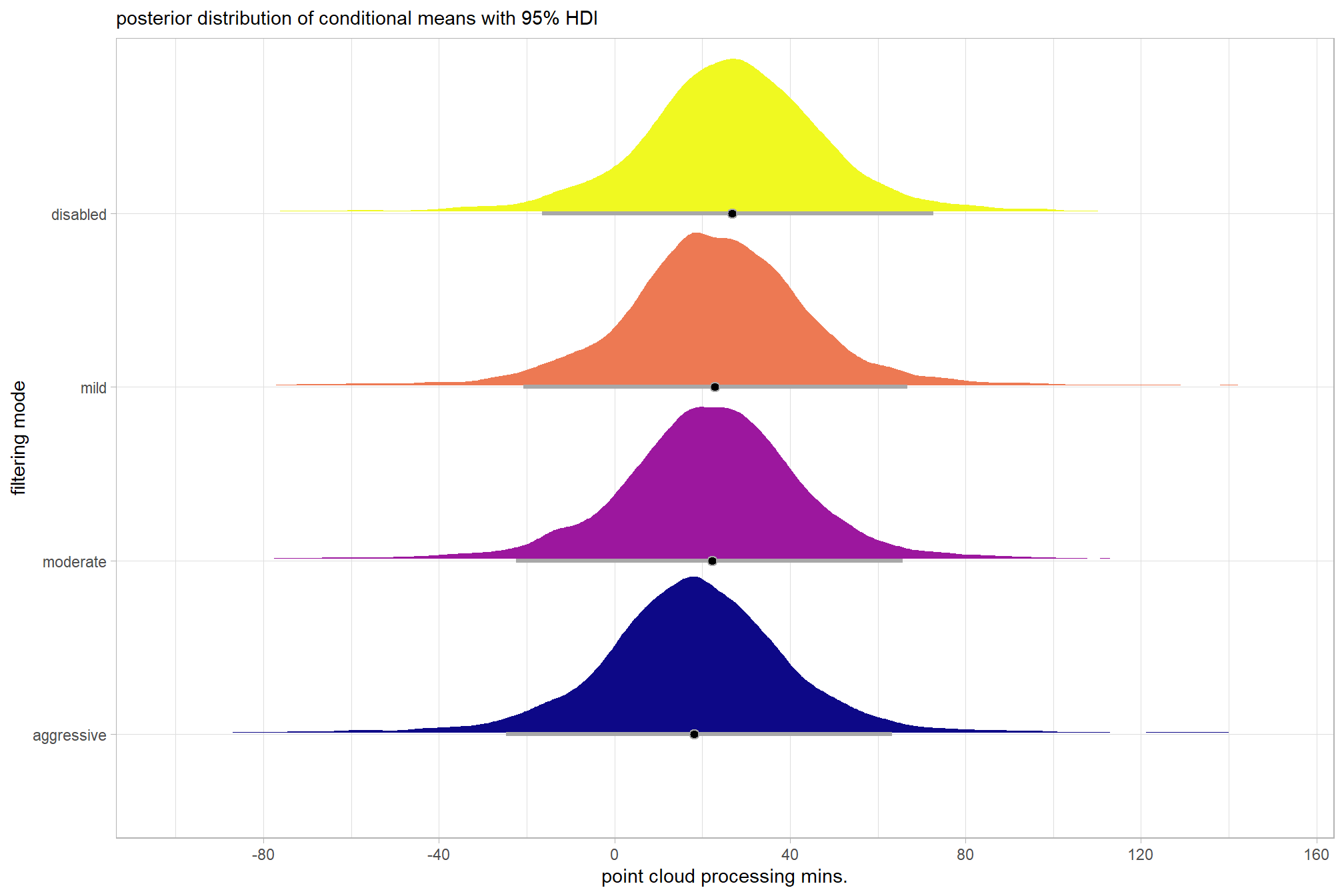
let’s compare these results to the results from our one nominal predictor model above and two nominal predictor model without site effects above
ptime_data %>%
  dplyr::distinct(depth_maps_generation_filtering_mode) %>%
  tidybayes::add_epred_draws(
    brms3_mod
    # this part is crucial
    , re_formula = ~ (1 | depth_maps_generation_filtering_mode)
  ) %>%
  dplyr::mutate(value = .epred, src = "site+two nominal predictor") %>%
  dplyr::bind_rows(
    ptime_data %>%
      dplyr::distinct(depth_maps_generation_filtering_mode) %>%
      tidybayes::add_epred_draws(
        brms2_mod
        # this part is crucial
        , re_formula = ~ (1 | depth_maps_generation_filtering_mode)
      ) %>%
      dplyr::mutate(value = .epred, src = "two nominal predictor")
  ) %>%
  ggplot(mapping = aes(y = src, x = value, color = src, group = src)) +
  tidybayes::stat_pointinterval(position = "dodge") +
  facet_grid(rows = vars(depth_maps_generation_filtering_mode), switch = "y") +
  scale_y_discrete(NULL, breaks = NULL) +
  scale_color_manual(values = viridis::turbo(n=4, begin = 0.2, end = 0.8)[3:4]) +
  labs(
    y = "filtering mode", x = "point cloud processing mins."
    , color = "model"
  ) +
  theme_light() +
  theme(legend.position = "top", strip.text = element_text(color = "black", face = "bold"))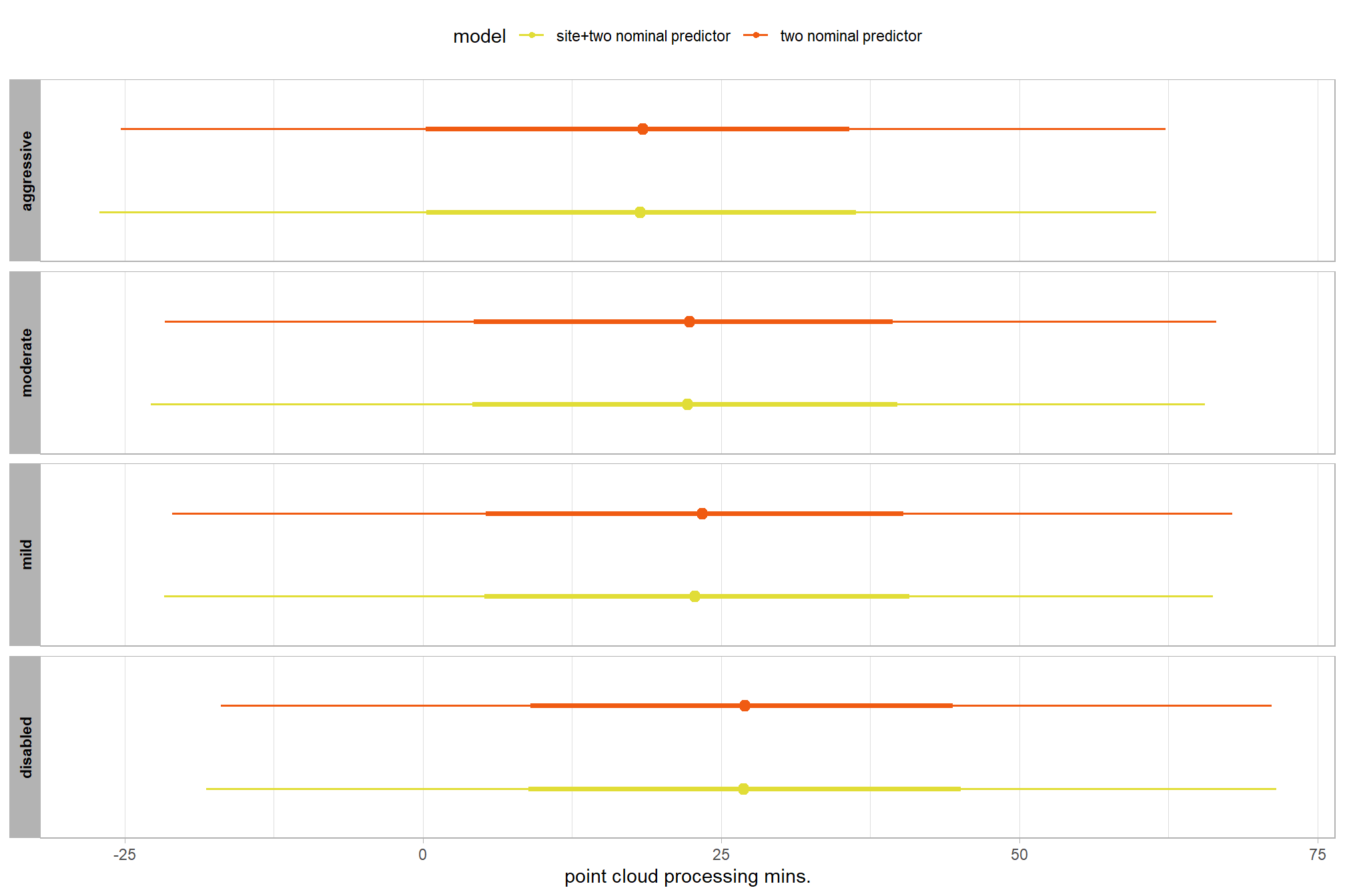
Finally, we can quantify the variation in processing time by comparing the \(\sigma\) posteriors.
# extract the posterior draws
brms::as_draws_df(brms3_mod) %>%
  dplyr::select(c(sigma,tidyselect::starts_with("sd_"))) %>%
  tidyr::pivot_longer(dplyr::everything()) %>%
  # dplyr::group_by(name) %>%
  # tidybayes::median_hdi(value) %>%
  dplyr::mutate(
    name = name %>%
      stringr::str_replace_all("depth_maps_generation_quality", "quality") %>%
      stringr::str_replace_all("depth_maps_generation_filtering_mode", "filtering") %>%
      forcats::fct_reorder(value)
  ) %>%
# plot
  ggplot(aes(x = value, y = name)) +
  tidybayes::stat_dotsinterval(
    point_interval = median_hdi, .width = .95
    , justification = -0.04
    , shape = 21 #, point_size = 3
    , quantiles = 100
  ) +
  labs(x = "", y = "") +
  theme_light()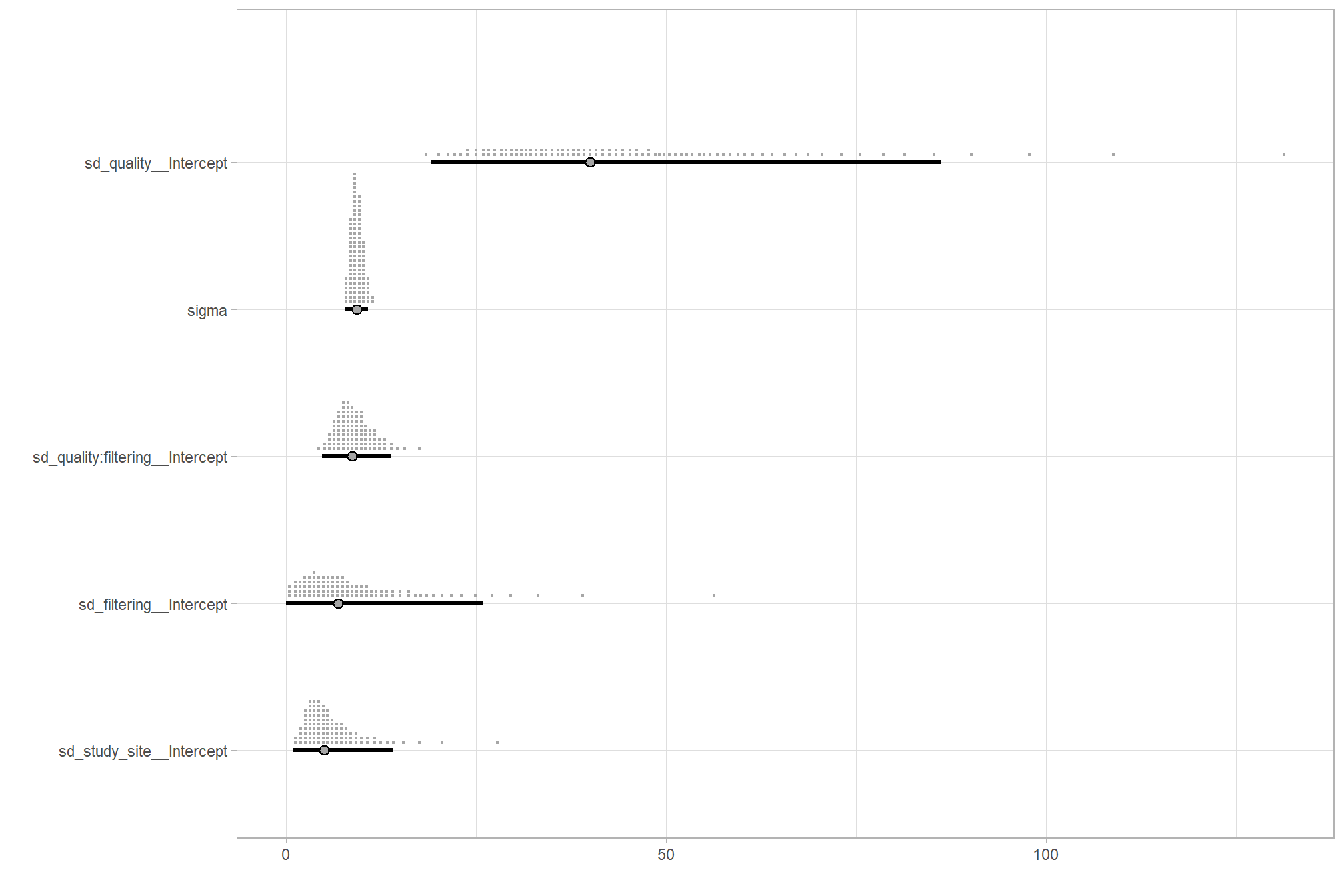
and perform model selection via information criteria with the brms::loo_compare() function
brms3_mod = brms::add_criterion(brms3_mod, criterion = c("loo", "waic"))
brms::loo_compare(brms1_mod, brms2_mod, brms3_mod, criterion = "loo")
## elpd_diff se_diff
## brms3_mod 0.0 0.0
## brms2_mod -6.6 2.4
## brms1_mod -23.0 11.44.4 Gamma: Two Nominal Predictors + site effects
To this point, we have been modelling point cloud processing time presuming a Gaussian likelihood. However, the gamma likelihood more accurately represents the processing time data which is continuous and strictly positive (i.e. it is impossible to have a negative runtime). The gamma distribution is a great alternative that accounts for data with a zero lower limit and any right skew.
We borrow here from the excellent series on causal inference by A. Solomon Kurz
4.4.1 Summary Statistics
let’s check our underlying data for point cloud processing time (our dependent or \(y\) variable)
# distribution
ptime_data %>%
  ggplot(mapping = aes(x = timer_total_time_mins)) +
  geom_hline(yintercept = 0) +
  geom_vline(xintercept = 0) +
  geom_density(fill = "lightblue", alpha = 0.7, color = NA) +
  labs(y="",x="point cloud processing mins.") +
  scale_y_continuous(breaks = c(0)) +
  theme_light() +
  theme(panel.grid = element_blank())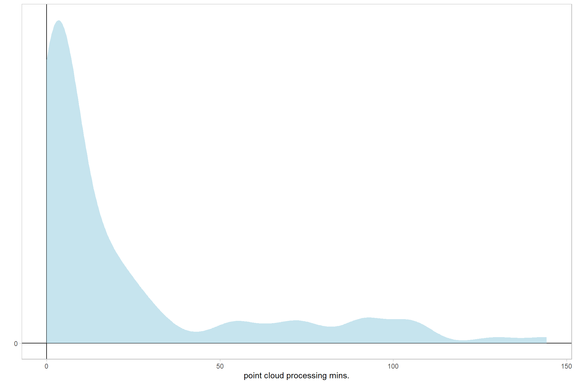
and the summary statistics
##    Min. 1st Qu.  Median    Mean 3rd Qu.    Max.
##   0.835   1.978   6.577  22.725  24.287 144.272
4.4.2 Bayesian
With the gamma likelihood our model becomes:
Need to check our prior selection…just go with brms defaults for now
\[\begin{align*} y_{i} &\sim {\sf Gamma} \bigl(\mu_{i}, \alpha \bigr) \\ log(\mu_{i}) &= \beta_0 + \sum_{j} \beta_{1[j]} x_{1[j]} + \sum_{k} \beta_{2[k]} x_{2[k]} + \sum_{j,k} \beta_{1\times2[j,k]} x_{1\times2[j,k]} + \sum_{s} \beta_{3[s]} x_{3[s]} \\ \beta_{0} &\sim {\sf Normal} (0,100) \\ \beta_{1[j]} &\sim {\sf Normal} (0,\sigma_{\beta_{1}}) \\ \beta_{2[k]} &\sim {\sf Normal} (0,\sigma_{\beta_{2}}) \\ \beta_{1\times2[j,k]} &\sim {\sf Normal} (0,\sigma_{\beta_{1\times2}}) \\ \beta_{3[s]} &\sim {\sf Normal} (0,\sigma_{\beta_{3}}) \\ \sigma_{\beta_{1}} &\sim {\sf Gamma} (1.28,0.005) \\ \sigma_{\beta_{2}} &\sim {\sf Gamma} (1.28,0.005) \\ \sigma_{\beta_{1\times2}} &\sim {\sf Gamma} (1.28,0.005) \\ \sigma_{\beta_{3}} &\sim {\sf Gamma} (1.28,0.005) \\ \alpha &\sim {\sf Gamma} (0.01,0.01) \\ \end{align*}\]
Note that the \({\sf Gamma}\) likelihood is parameterized in terms of the mean (\(\mu\)) and the shape (\(\alpha\))
Now fit the model.
brms4_mod = brms::brm(
  formula = timer_total_time_mins ~ 1 +
    (1 | depth_maps_generation_quality) +
    (1 | depth_maps_generation_filtering_mode) +
    (1 | depth_maps_generation_quality:depth_maps_generation_filtering_mode) +
    (1 | study_site)
  , data = ptime_data
  , family = brms::brmsfamily("Gamma", link = "log") # Gamma(link = "log")
  , iter = 4000, warmup = 2000, chains = 4
  , cores = round(parallel::detectCores()/2)
  # , prior = c(
  #   brms::prior(normal(mean_y, sd_y * 5), class = "Intercept")
  #   , brms::prior(gamma(alpha, beta), class = "sd")
  #   , brms::prior(cauchy(0, sd_y), class = "sigma")
  # )
  # , stanvars = stanvars_temp
  , file = paste0(rootdir, "/fits/brms4_mod")
)
check the trace plots for problems with convergence of the Markov chains
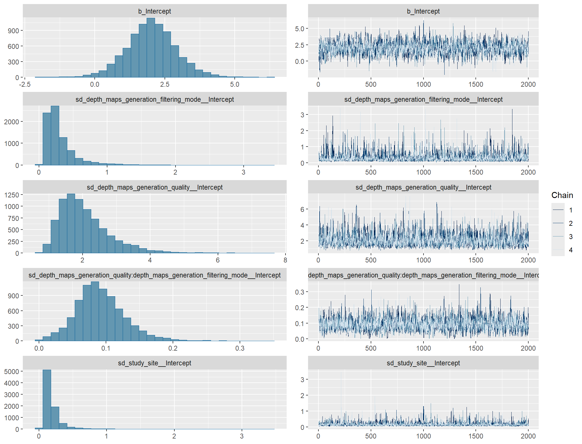
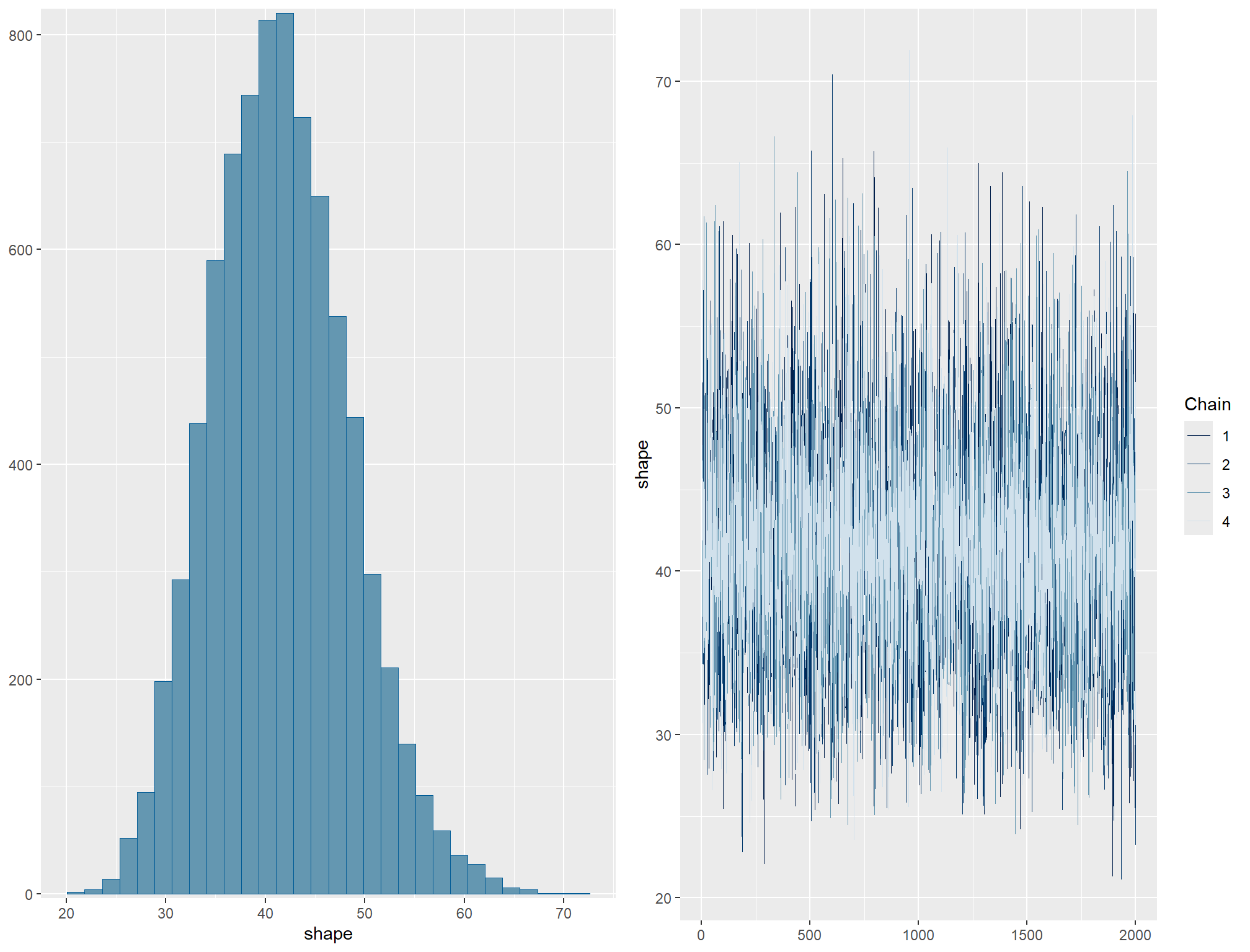
posterior-predictive check to make sure the model does an okay job simulating data that resemble the sample data
# posterior predictive check
brms::pp_check(
    brms4_mod
    , type = "dens_overlay"
    , ndraws = 50
  ) +
  labs(subtitle = "posterior-predictive check (overlaid densities)") +
  theme_light() +
  theme(legend.position = "top", legend.direction = "horizontal", legend.text = element_text(size = 14))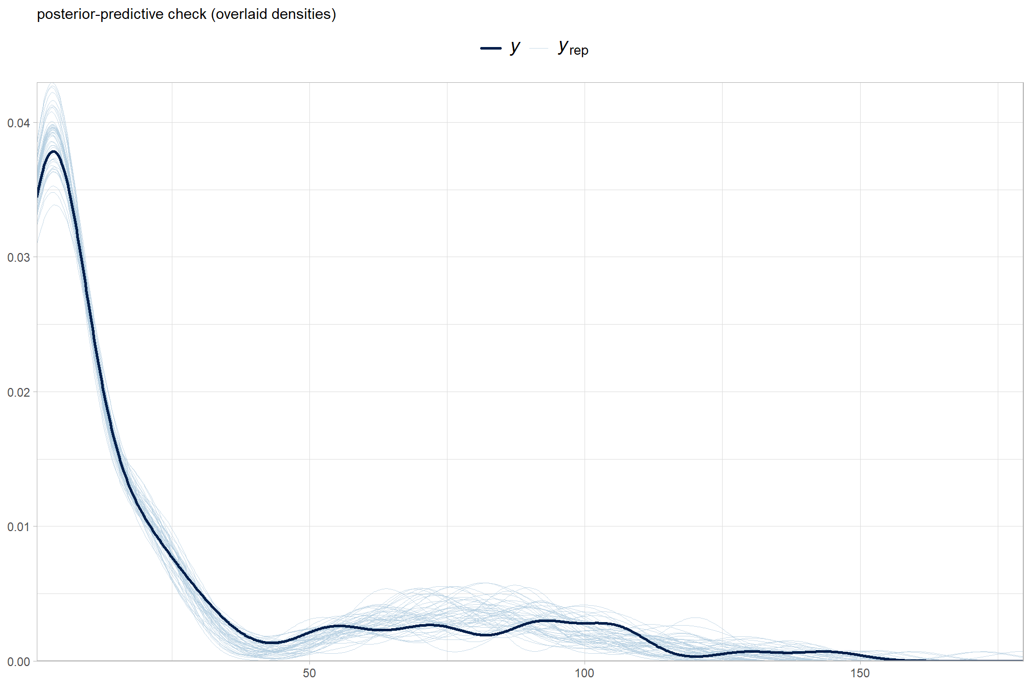
How’d we do capturing the conditional means and standard deviations by depth map generation quality?
# means
p1_temp = brms::pp_check(
    brms4_mod
    , type = "stat_grouped" # "dens_overlay_grouped"
    , stat = "mean"
    , group = "depth_maps_generation_quality"
  ) +
  scale_y_continuous(NULL, breaks = c(NULL)) +
  labs(subtitle = "means") +
  facet_grid(cols = vars(group), scales = "free") +
  theme_light()
# sds
p2_temp = brms::pp_check(
    brms4_mod
    , type = "stat_grouped" # "dens_overlay_grouped"
    , stat = "sd"
    , group = "depth_maps_generation_quality"
  ) +
  scale_y_continuous(NULL, breaks = c(NULL)) +
  labs(subtitle = "sd's") +
  facet_grid(cols = vars(group), scales = "free") +
  theme_light()
# combine
(p1_temp / p2_temp) &
  theme(legend.position = "none") &
  plot_annotation(
    title = "Posterior-predictive statistical checks\nby depth map quality"
    , subtitle = expression(
      "The dark blue lines are "*italic(T(y))*", and the light blue bars are for "*italic(T)(italic(y)[rep])*".")
  )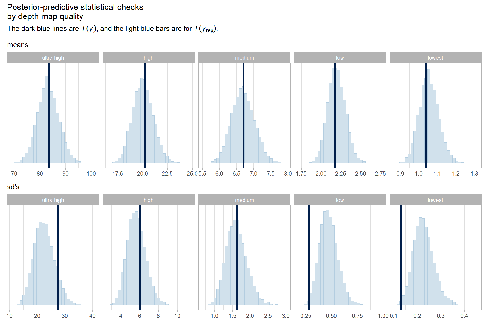
The means are decent, the sd’s are terrible…see the section “Heterogeneous variances and robustness against outliers” in Kruschke (2015) on p.602 and in Kurz’s ebook companion
check the prior distributions
| prior | class | coef | group | resp | dpar | nlpar | lb | ub | source |
|---|---|---|---|---|---|---|---|---|---|
| student_t(3, 1.9, 2.5) | Intercept | default | |||||||
| student_t(3, 0, 2.5) | sd | 0 | default | ||||||
| sd | depth_maps_generation_filtering_mode | default | |||||||
| sd | Intercept | depth_maps_generation_filtering_mode | default | ||||||
| sd | depth_maps_generation_quality | default | |||||||
| sd | Intercept | depth_maps_generation_quality | default | ||||||
| sd | depth_maps_generation_quality:depth_maps_generation_filtering_mode | default | |||||||
| sd | Intercept | depth_maps_generation_quality:depth_maps_generation_filtering_mode | default | ||||||
| sd | study_site | default | |||||||
| sd | Intercept | study_site | default | ||||||
| gamma(0.01, 0.01) | shape | 0 | default |
The brms::brm model summary
brms4_mod %>%
  brms::posterior_summary() %>%
  as.data.frame() %>%
  tibble::rownames_to_column(var = "parameter") %>%
  dplyr::rename_with(tolower) %>%
  dplyr::filter(
    stringr::str_starts(parameter, "b_")
    | stringr::str_starts(parameter, "r_")
    | stringr::str_starts(parameter, "sd_")
    | parameter == "shape"
  ) %>%
  dplyr::mutate(
    parameter = parameter %>%
      stringr::str_replace_all("depth_maps_generation_quality", "quality") %>%
      stringr::str_replace_all("depth_maps_generation_filtering_mode", "filtering")
  ) %>%
  kableExtra::kbl(digits = 2, caption = "Bayesian two nominal predictors + study site effects for point cloud processing time") %>%
  kableExtra::kable_styling() %>%
kableExtra::scroll_box(height = "6in")| parameter | estimate | est.error | q2.5 | q97.5 |
|---|---|---|---|---|
| b_Intercept | 2.02 | 0.89 | 0.25 | 3.82 |
| sd_filtering__Intercept | 0.31 | 0.26 | 0.09 | 1.04 |
| sd_quality__Intercept | 2.07 | 0.78 | 1.06 | 4.01 |
| sd_quality:filtering__Intercept | 0.09 | 0.04 | 0.02 | 0.18 |
| sd_study_site__Intercept | 0.18 | 0.12 | 0.06 | 0.49 |
| shape | 41.53 | 6.81 | 29.30 | 55.69 |
| r_filtering[aggressive,Intercept] | -0.18 | 0.20 | -0.57 | 0.20 |
| r_filtering[moderate,Intercept] | -0.03 | 0.20 | -0.42 | 0.37 |
| r_filtering[mild,Intercept] | 0.03 | 0.19 | -0.35 | 0.43 |
| r_filtering[disabled,Intercept] | 0.19 | 0.20 | -0.17 | 0.60 |
| r_quality[ultra.high,Intercept] | 2.38 | 0.87 | 0.58 | 4.11 |
| r_quality[high,Intercept] | 0.95 | 0.87 | -0.86 | 2.68 |
| r_quality[medium,Intercept] | -0.13 | 0.87 | -1.93 | 1.59 |
| r_quality[low,Intercept] | -1.24 | 0.87 | -3.04 | 0.48 |
| r_quality[lowest,Intercept] | -1.97 | 0.87 | -3.77 | -0.23 |
| r_quality:filtering[high_aggressive,Intercept] | -0.09 | 0.08 | -0.28 | 0.05 |
| r_quality:filtering[high_disabled,Intercept] | 0.09 | 0.08 | -0.05 | 0.27 |
| r_quality:filtering[high_mild,Intercept] | 0.02 | 0.08 | -0.13 | 0.17 |
| r_quality:filtering[high_moderate,Intercept] | -0.01 | 0.07 | -0.16 | 0.14 |
| r_quality:filtering[low_aggressive,Intercept] | 0.07 | 0.08 | -0.07 | 0.24 |
| r_quality:filtering[low_disabled,Intercept] | -0.06 | 0.08 | -0.22 | 0.08 |
| r_quality:filtering[low_mild,Intercept] | -0.01 | 0.07 | -0.16 | 0.14 |
| r_quality:filtering[low_moderate,Intercept] | -0.01 | 0.07 | -0.16 | 0.13 |
| r_quality:filtering[lowest_aggressive,Intercept] | 0.06 | 0.08 | -0.09 | 0.23 |
| r_quality:filtering[lowest_disabled,Intercept] | -0.06 | 0.08 | -0.23 | 0.08 |
| r_quality:filtering[lowest_mild,Intercept] | 0.00 | 0.08 | -0.16 | 0.15 |
| r_quality:filtering[lowest_moderate,Intercept] | 0.00 | 0.07 | -0.16 | 0.14 |
| r_quality:filtering[medium_aggressive,Intercept] | 0.01 | 0.07 | -0.14 | 0.17 |
| r_quality:filtering[medium_disabled,Intercept] | 0.02 | 0.08 | -0.12 | 0.19 |
| r_quality:filtering[medium_mild,Intercept] | -0.02 | 0.08 | -0.18 | 0.13 |
| r_quality:filtering[medium_moderate,Intercept] | -0.01 | 0.07 | -0.16 | 0.14 |
| r_quality:filtering[ultra.high_aggressive,Intercept] | -0.10 | 0.08 | -0.29 | 0.04 |
| r_quality:filtering[ultra.high_disabled,Intercept] | 0.06 | 0.08 | -0.08 | 0.23 |
| r_quality:filtering[ultra.high_mild,Intercept] | 0.02 | 0.08 | -0.12 | 0.18 |
| r_quality:filtering[ultra.high_moderate,Intercept] | 0.03 | 0.07 | -0.12 | 0.19 |
| r_study_site[KAIBAB_HIGH,Intercept] | 0.01 | 0.10 | -0.18 | 0.21 |
| r_study_site[KAIBAB_LOW,Intercept] | -0.13 | 0.10 | -0.33 | 0.06 |
| r_study_site[N1,Intercept] | 0.08 | 0.10 | -0.11 | 0.27 |
| r_study_site[SQ09_02,Intercept] | 0.12 | 0.10 | -0.07 | 0.32 |
| r_study_site[WA85_02,Intercept] | -0.08 | 0.10 | -0.28 | 0.11 |
We can look at the model noise standard deviation (shape) \(\alpha\)
# extract the posterior draws
brms::as_draws_df(brms4_mod) %>%
# plot
  ggplot(aes(x = shape, y = 0)) +
  tidybayes::stat_dotsinterval(
    point_interval = median_hdi, .width = .95
    , justification = -0.04
    , shape = 21, point_size = 3
    , quantiles = 100
  ) +
  scale_y_continuous(NULL, breaks = NULL) +
  xlab(latex2exp::TeX("$\\alpha$")) +
  theme_light()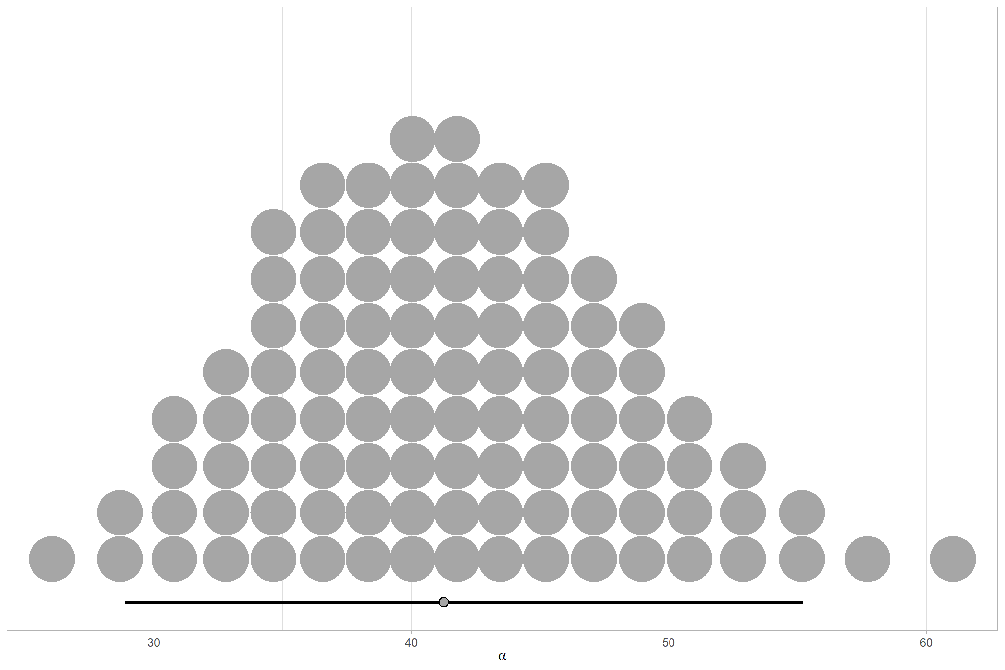
plot the posterior distributions of the conditional means with the median processing time and the 95% highest posterior density interval (HDI)
Note that how within tidybayes::add_epred_draws, we used the re_formula argument to average over the random effects of study_site (i.e., we left (1 | study_site) out of the formula). For this model we have to collapse across the study site effects to compare the depth map quality and filtering mode setting effects.
ptime_data %>%
  dplyr::distinct(depth_maps_generation_quality, depth_maps_generation_filtering_mode) %>%
  tidybayes::add_epred_draws(
    brms4_mod, allow_new_levels = T
    # this part is crucial
    , re_formula = ~ (1 | depth_maps_generation_quality) +
      (1 | depth_maps_generation_filtering_mode) +
      (1 | depth_maps_generation_quality:depth_maps_generation_filtering_mode)
  ) %>%
  dplyr::rename(value = .epred) %>%
  dplyr::mutate(depth_maps_generation_quality = depth_maps_generation_quality %>% forcats::fct_rev()) %>%
  # plot
  ggplot(
    mapping = aes(
      y = value, x = depth_maps_generation_filtering_mode
      , fill = depth_maps_generation_filtering_mode
    )
  ) +
    tidybayes::stat_eye(
      point_interval = median_hdi, .width = .95
      , slab_alpha = 0.8
      , interval_color = "black", linewidth = 1
      , point_color = "black", point_fill = "black", point_size = 1
    ) +
    scale_fill_viridis_d(option = "plasma", drop = F) +
    scale_y_log10(
      labels = scales::comma_format(suffix = " mins", accuracy = 1)
      , breaks = scales::breaks_log(n = 8)
    ) +
    facet_grid(cols = vars(depth_maps_generation_quality)) +
    labs(
      x = "filtering mode", y = "point cloud processing mins."
      , subtitle = "posterior distribution of conditional means with 95% HDI"
      , fill = "Filtering Mode"
    ) +
    theme_light() +
    theme(
      legend.position = "none"
      , legend.direction  = "horizontal"
      , axis.text.x = element_text(angle = 90, vjust = 0.5, hjust = 1)
      , strip.text = element_text(color = "black", face = "bold")
) 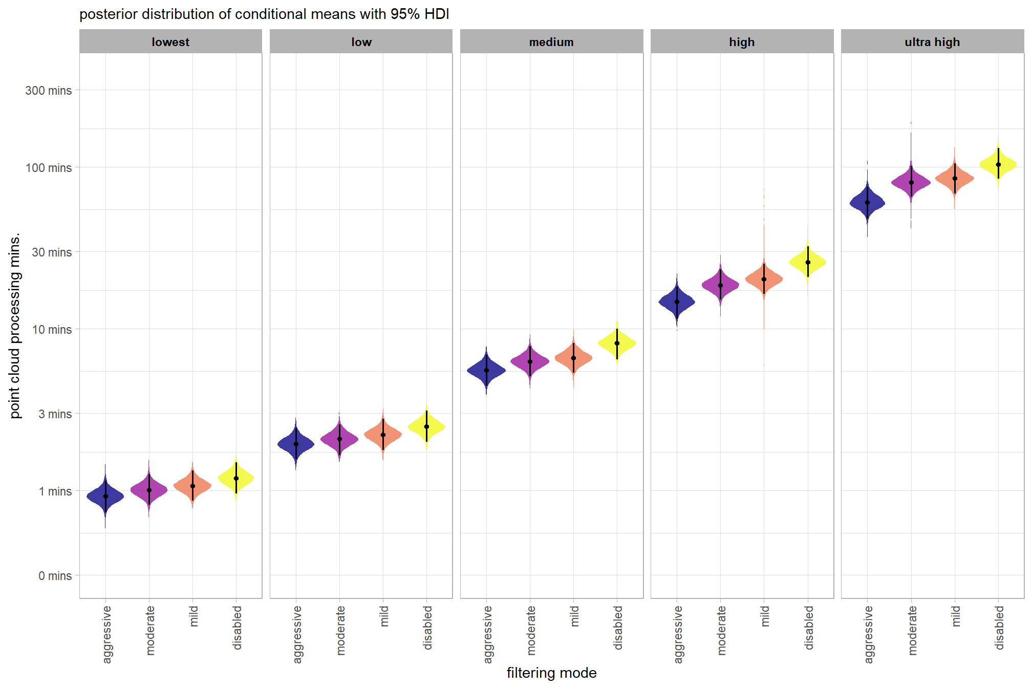
    # guides(
    #   fill = guide_legend(reverse = T, override.aes = list(alpha = 1, color = NA, shape = NA, lwd = NA))
    # )
That really tightened-up our estimates. Note that we had to use a log scale on the y axis (using ggplot2::scale_y_log10) and that none of our estimates for processing time are below zero.
we can also make pairwise comparisons so long as we continue using tidybayes::add_epred_draws with the re_formula argument
brms_contrast_temp =
  ptime_data %>%
    dplyr::distinct(depth_maps_generation_quality, depth_maps_generation_filtering_mode) %>%
    tidybayes::add_epred_draws(
      brms4_mod, allow_new_levels = T
      # this part is crucial
      , re_formula = ~ (1 | depth_maps_generation_quality) +
        (1 | depth_maps_generation_filtering_mode) +
        (1 | depth_maps_generation_quality:depth_maps_generation_filtering_mode)
    ) %>%
    dplyr::rename(value = .epred) %>%
    tidybayes::compare_levels(
      value
      , by = depth_maps_generation_quality
      , comparison =
        contrast_list
        # tidybayes::emmeans_comparison("revpairwise")
        #"pairwise"
    ) %>%
    dplyr::rename(contrast = depth_maps_generation_quality)

# separate contrast
brms_contrast_temp = brms_contrast_temp %>%
  dplyr::ungroup() %>%
  tidyr::separate_wider_delim(
    cols = contrast
    , delim = " - "
    , names = paste0(
        "sorter"
        , 1:(max(stringr::str_count(brms_contrast_temp$contrast, "-"))+1)
      )
    , too_few = "align_start"
    , cols_remove = F
  ) %>%
  dplyr::filter(sorter1!=sorter2) %>%
  dplyr::mutate(
    dplyr::across(
      tidyselect::starts_with("sorter")
      , .fns = function(x){factor(
        x, ordered = T
        , levels = levels(ptime_data$depth_maps_generation_quality)
      )}
    )
    , contrast = contrast %>%
      forcats::fct_reorder(
        paste0(as.numeric(sorter1), as.numeric(sorter2)) %>%
        as.numeric()
      )
    , depth_maps_generation_filtering_mode = depth_maps_generation_filtering_mode %>%
      factor(
        levels = levels(ptime_data$depth_maps_generation_filtering_mode)
        , ordered = T
      )
  ) %>%
  # median_hdi summary for coloring
  dplyr::group_by(contrast, depth_maps_generation_filtering_mode) %>%
  dplyr::mutate(
    is_gt_zero = value > 0
    , pct_gt_zero = sum(is_gt_zero)/dplyr::n()
    , sig_level2 = dplyr::case_when(
      pct_gt_zero > 0.99 ~ 0
      , pct_gt_zero > 0.95 ~ 1
      , pct_gt_zero > 0.9 ~ 2
      , pct_gt_zero > 0.8 ~ 3
      , T ~ 4
    ) %>%
    factor(levels = c(0:4), labels = c(">99%","95%","90%","80%","<80%"), ordered = T)
  )

# what?
brms_contrast_temp %>% dplyr::glimpse()
## Rows: 320,000
## Columns: 11
## Groups: contrast, depth_maps_generation_filtering_mode [40]
## $ depth_maps_generation_filtering_mode <ord> aggressive, aggressive, aggressiv…
## $ .chain <int> NA, NA, NA, NA, NA, NA, NA, NA, N…
## $ .iteration <int> NA, NA, NA, NA, NA, NA, NA, NA, N…
## $ .draw <int> 1, 2, 3, 4, 5, 6, 7, 8, 9, 10, 11…
## $ sorter1 <ord> ultra high, ultra high, ultra hig…
## $ sorter2 <ord> high, high, high, high, high, hig…
## $ contrast <fct> ultra high - high, ultra high - h…
## $ value <dbl> 53.82774, 42.97583, 42.28363, 46.…
## $ is_gt_zero <lgl> TRUE, TRUE, TRUE, TRUE, TRUE, TRU…
## $ pct_gt_zero <dbl> 1, 1, 1, 1, 1, 1, 1, 1, 1, 1, 1, …
## $ sig_level2 <ord> >99%, >99%, >99%, >99%, >99%, >99…plot it with the help of ggplot2::scale_x_log10
# plot it
brms_contrast_temp %>%
  ggplot(
    mapping = aes(
      x = value, y = contrast
      , fill = sig_level2 # pct_gt_zero
      # , fill = depth_maps_generation_filtering_mode
    )
  ) +
    # # for kicks and giggles we'll throw in the ROPE
    geom_vline(xintercept = 0.1, linetype = "dashed", color = "gray44", lwd = 1) +
    tidybayes::stat_halfeye(
      point_interval = median_hdi, .width = c(0.5,0.95)
      # , slab_fill = "gray22", slab_alpha = 1
      , interval_color = "black", point_color = "black", point_fill = "black"
      , justification = -0.01
    ) +
    scale_fill_viridis_d(
      option = "mako", begin = 0.3
      , drop = F
      # , labels = scales::percent
    ) +
    # scale_fill_viridis_c(
    #   option = "mako", begin = 0.3, direction = -1
    #   , labels = scales::percent
    # ) +
    scale_x_log10(
      labels = scales::comma_format(suffix = " mins", accuracy = 1)
      , breaks = c(0.1,1,3,10,30,100,300,800)
        # scales::breaks_log(n = 8)
    ) +
    facet_grid(cols = vars(depth_maps_generation_filtering_mode)) +
    labs(
      y = "depth map quality"
      , x = "constrast (mins.)"
      , subtitle = "95% & 50% HDI of the posterior distribution of conditional mean group constrasts"
      , fill = "Pr(contrast > 0)"
    ) +
    theme_light() +
    theme(
      legend.position = "top"
      , legend.direction  = "horizontal"
      , axis.text.x = element_text(angle = 45, hjust = 1)
      , strip.text = element_text(color = "black", face = "bold")
    ) +
    guides(
      fill = guide_legend(reverse = T, override.aes = list(alpha = 1, color = NA, shape = NA, lwd = NA))
    )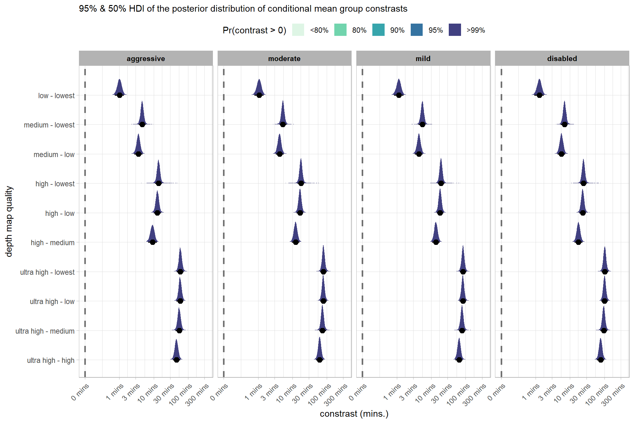
and summarize these contrasts
brms_contrast_temp %>%
  dplyr::group_by(contrast, depth_maps_generation_filtering_mode) %>%
  tidybayes::median_hdi(value) %>%
  dplyr::arrange(contrast, depth_maps_generation_filtering_mode) %>%
  dplyr::select(contrast, depth_maps_generation_filtering_mode, value, .lower, .upper) %>%
  dplyr::rename(difference=value) %>%
kableExtra::kbl(
    digits = 1
    , caption = "brms::brm model: 95% HDI of the posterior distribution of conditional mean group constrasts"
    , col.names = c(
      "quality contrast"
      , "filtering mode"
      , "difference (mins.)"
      , "conf.low", "conf.high"
    )
  ) %>%
  kableExtra::kable_styling() %>%
kableExtra::scroll_box(height = "6in")| quality contrast | filtering mode | difference (mins.) | conf.low | conf.high |
|---|---|---|---|---|
| ultra high - high | aggressive | 45.8 | 35.1 | 58.5 |
| ultra high - high | moderate | 61.9 | 47.0 | 77.1 |
| ultra high - high | mild | 64.7 | 49.3 | 80.5 |
| ultra high - high | disabled | 77.9 | 60.0 | 97.9 |
| ultra high - medium | aggressive | 55.0 | 43.2 | 69.1 |
| ultra high - medium | moderate | 74.2 | 58.7 | 92.5 |
| ultra high - medium | mild | 78.5 | 62.2 | 97.1 |
| ultra high - medium | disabled | 95.7 | 75.5 | 118.6 |
| ultra high - low | aggressive | 58.5 | 45.7 | 72.7 |
| ultra high - low | moderate | 78.4 | 63.2 | 98.2 |
| ultra high - low | mild | 82.9 | 65.2 | 101.3 |
| ultra high - low | disabled | 101.4 | 80.2 | 125.0 |
| ultra high - lowest | aggressive | 59.6 | 46.8 | 74.0 |
| ultra high - lowest | moderate | 79.5 | 64.1 | 99.5 |
| ultra high - lowest | mild | 84.0 | 66.7 | 103.0 |
| ultra high - lowest | disabled | 102.7 | 81.8 | 127.0 |
| high - medium | aggressive | 9.2 | 6.4 | 11.8 |
| high - medium | moderate | 12.3 | 9.3 | 15.7 |
| high - medium | mild | 13.7 | 10.4 | 17.4 |
| high - medium | disabled | 17.6 | 13.3 | 22.6 |
| high - low | aggressive | 12.8 | 9.7 | 15.9 |
| high - low | moderate | 16.6 | 13.0 | 20.4 |
| high - low | mild | 18.1 | 14.2 | 22.4 |
| high - low | disabled | 23.3 | 18.2 | 29.0 |
| high - lowest | aggressive | 13.8 | 10.7 | 17.1 |
| high - lowest | moderate | 17.6 | 13.9 | 21.7 |
| high - lowest | mild | 19.3 | 15.2 | 23.7 |
| high - lowest | disabled | 24.6 | 19.7 | 30.8 |
| medium - low | aggressive | 3.6 | 2.7 | 4.6 |
| medium - low | moderate | 4.2 | 3.2 | 5.3 |
| medium - low | mild | 4.4 | 3.3 | 5.5 |
| medium - low | disabled | 5.6 | 4.3 | 7.2 |
| medium - lowest | aggressive | 4.6 | 3.6 | 5.7 |
| medium - lowest | moderate | 5.3 | 4.2 | 6.6 |
| medium - lowest | mild | 5.5 | 4.3 | 6.8 |
| medium - lowest | disabled | 6.9 | 5.4 | 8.6 |
| low - lowest | aggressive | 1.0 | 0.7 | 1.4 |
| low - lowest | moderate | 1.1 | 0.8 | 1.4 |
| low - lowest | mild | 1.1 | 0.8 | 1.5 |
| low - lowest | disabled | 1.3 | 0.9 | 1.7 |
let’s collapse across the filtering mode and study site to compare the depth map quality setting effect.
In a hierarchical model structure, we have to make use of the re_formula argument within tidybayes::add_epred_draws
we continue to use ggplot2::scale_x_log10
ptime_data %>%
  dplyr::distinct(depth_maps_generation_quality) %>%
  tidybayes::add_epred_draws(
    brms4_mod
    # this part is crucial
    , re_formula = ~ (1 | depth_maps_generation_quality)
  ) %>%
  dplyr::rename(value = .epred) %>%
  # plot
  ggplot(
    mapping = aes(
      x = value, y = depth_maps_generation_quality
      , fill = depth_maps_generation_quality
    )
  ) +
    geom_vline(xintercept = 0.1, linetype = "dashed", color = "gray44", lwd = 1) +
    tidybayes::stat_dotsinterval(quantiles = 100) +
    # tidybayes::stat_halfeye(
    #   point_interval = median_hdi, .width = .95
    #   , interval_color = "gray66"
    #   , shape = 21, point_color = "gray66", point_fill = "black"
    #   , justification = -0.01
    # ) +
    scale_fill_viridis_d(option = "inferno", drop = F) +
    scale_x_log10(
      labels = scales::comma_format(suffix = " mins", accuracy = 1)
      , breaks = c(0.1,1,3,10,30,100,300,1000)
    ) +
    labs(
      y = "depth map quality", x = "point cloud processing mins."
      , subtitle = "posterior distribution of conditional means with 95% HDI"
    ) +
    theme_light() +
    theme(legend.position = "none", axis.text.x = element_text(angle = 45, hjust = 1))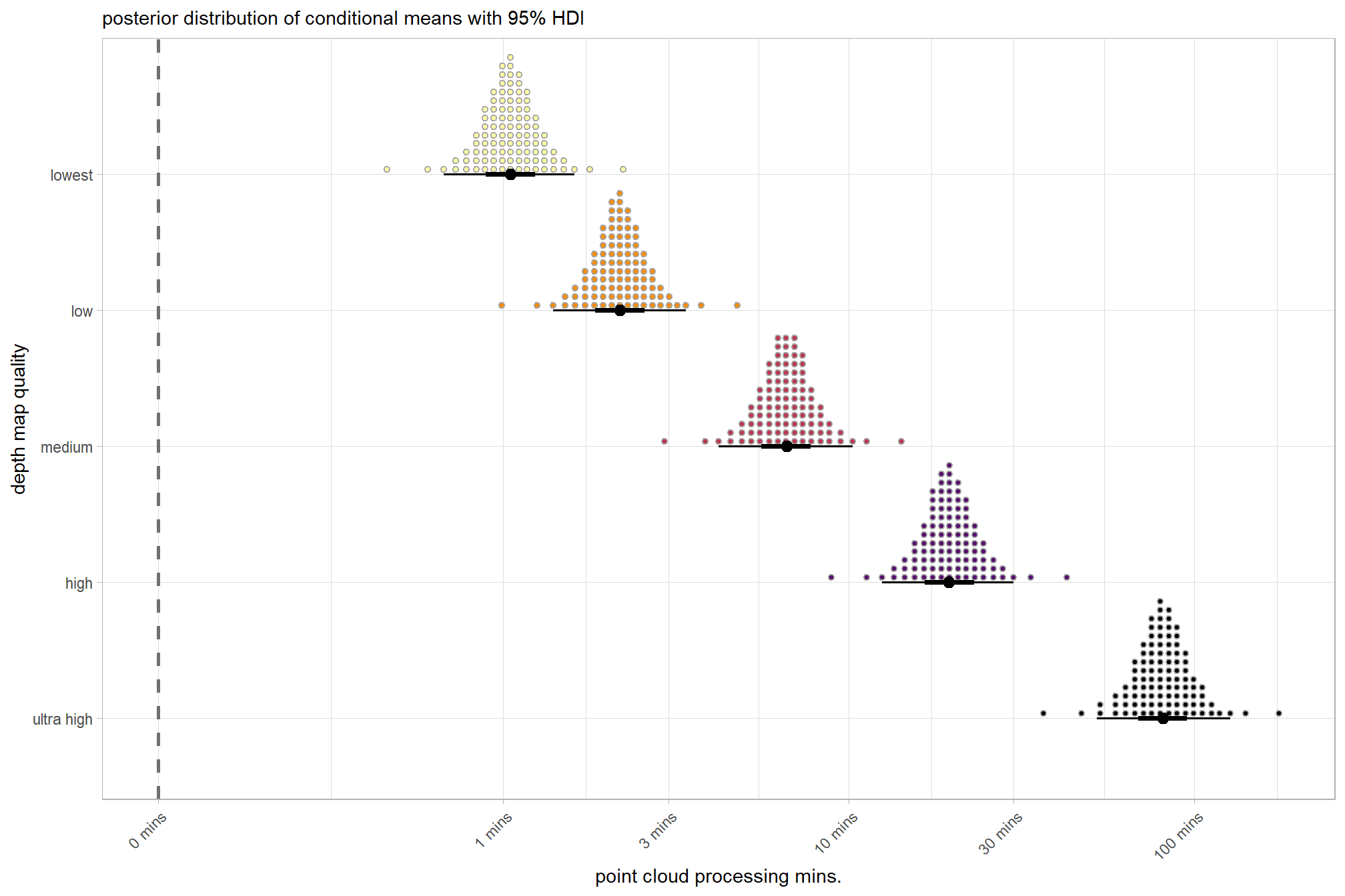
let’s compare these results to the results from our one nominal predictor model above and two nominal predictor model without site effects above and two nominal predictor model with site effects above
ptime_data %>%
  dplyr::distinct(depth_maps_generation_quality) %>%
  tidybayes::add_epred_draws(
    brms4_mod
    # this part is crucial
    , re_formula = ~ (1 | depth_maps_generation_quality)
  ) %>%
  dplyr::mutate(value = .epred, src = "site+two nominal predictor: gamma") %>%
  dplyr::bind_rows(
    ptime_data %>%
      dplyr::distinct(depth_maps_generation_quality) %>%
      tidybayes::add_epred_draws(
        brms3_mod
        # this part is crucial
        , re_formula = ~ (1 | depth_maps_generation_quality)
      ) %>%
      dplyr::mutate(value = .epred, src = "site+two nominal predictor: gauss")
    , ptime_data %>%
      dplyr::distinct(depth_maps_generation_quality) %>%
      tidybayes::add_epred_draws(
        brms2_mod
        # this part is crucial
        , re_formula = ~ (1 | depth_maps_generation_quality)
      ) %>%
      dplyr::mutate(value = .epred, src = "two nominal predictor")
    , ptime_data %>%
      dplyr::distinct(depth_maps_generation_quality) %>%
      tidybayes::add_epred_draws(brms1_mod) %>%
      dplyr::mutate(value = .epred, src = "one nominal predictor")
  ) %>%
  ggplot(mapping = aes(y = src, x = value, color = src, group = src)) +
  geom_vline(xintercept = 0, linetype = "dashed", color = "gray44") +
  tidybayes::stat_pointinterval(position = "dodge") +
  facet_grid(rows = vars(depth_maps_generation_quality), switch = "y") +
  scale_y_discrete(NULL, breaks = NULL) +
  scale_x_continuous(breaks = scales::extended_breaks(10)) +
  scale_color_viridis_d(option = "turbo", begin = 0.2, end = 0.8) +
  labs(
    y = "", x = "point cloud processing mins."
    , color = "model"
  ) +
  theme_light() +
  theme(
    legend.position = "top", strip.text = element_text(color = "black", face = "bold")
  ) +
  guides(
    color = guide_legend(
      nrow = 2, byrow = T
      , override.aes = list(shape = 15, size = 10, lwd = NA)
    )
  )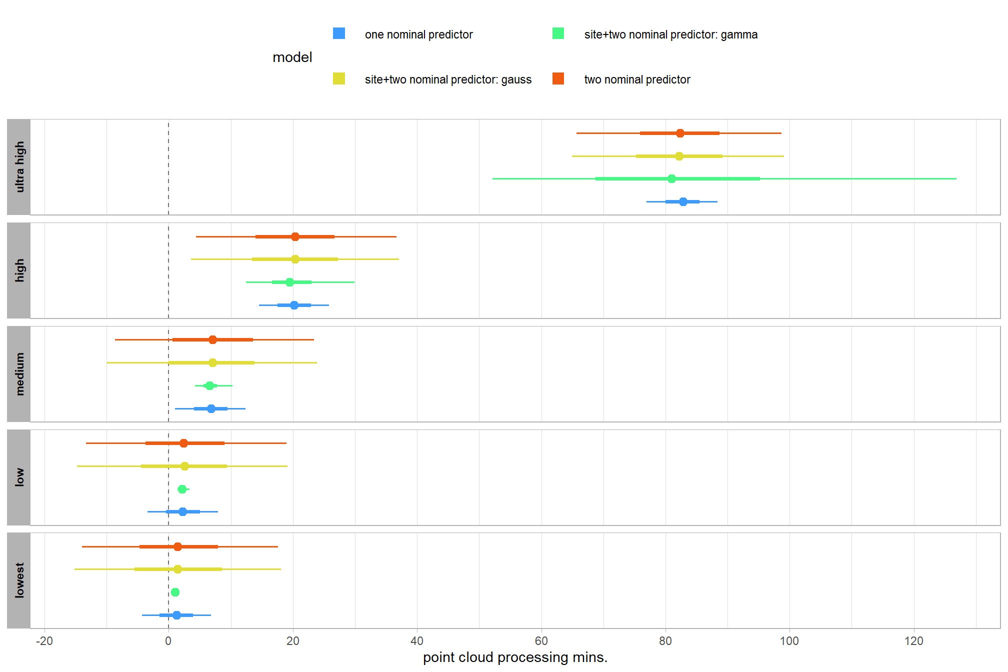
Notice that our gamma likelihood model constrains the processing time estimate to strictly positive values while the other models which utilized a Gaussian likelihood predict nonsensical negative processing times. The gamma distribution also does a nice job representing the right-skew observed in the processing time data.
Let’s check the posterior distribution for the overall grand mean \(\beta_{0}\) to see how well the right-skew is represented (we also saw this in our posterior predictive checks). We’ll make use of brms::fixef and we use the \(exp()\) to transform the predicted values because we are using the log link with the gamma likelihood
# we can make use of brms::fixef
brms::fixef(brms4_mod, summary = F) %>%
  dplyr::as_tibble() %>%
  dplyr::ungroup() %>%
  dplyr::mutate(value = exp(Intercept)) %>%
  # plot
  ggplot(aes(x = value, y = 0)) +
    geom_vline(xintercept = 0) +
    tidybayes::stat_dotsinterval(
      point_interval = median_hdi, .width = .95
      , justification = -0.04
      , shape = 21, point_size = 3
      , quantiles = 100
    ) +
    labs(y="",x="point cloud processing mins.", subtitle = latex2exp::TeX("gamma likelihood model posterior distribution of the grand mean $\\beta_0$")) +
    scale_y_continuous(NULL, breaks = NULL) +
    scale_x_continuous(breaks = scales::extended_breaks(15)) +
    theme_light()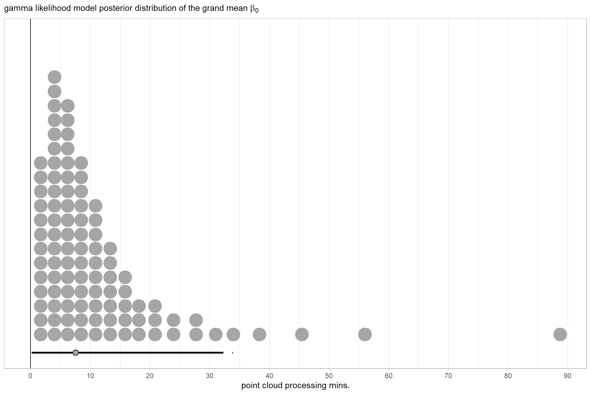
and get the summary statistics of the grand mean using brms::as_draws_df and posterior::summarise_draws
brms::as_draws_df(brms4_mod) %>%
  select(b_Intercept) %>%
  dplyr::mutate(b_Intercept = exp(b_Intercept)) %>%
  posterior::summarise_draws() %>%
  kableExtra::kbl(digits = 1, caption = "brms::brm model: summary statiscits of the grand mean") %>%
kableExtra::kable_styling()| variable | mean | median | sd | mad | q5 | q95 | rhat | ess_bulk | ess_tail |
|---|---|---|---|---|---|---|---|---|---|
| b_Intercept | 11.4 | 7.5 | 15.6 | 5.7 | 1.8 | 32.4 | 1 | 2117.1 | 3176.9 |
For completeness, let’s also collapse across the depth map quality to compare the filtering mode setting effect.
In a hierarchical model structure, we have to make use of the re_formula argument within tidybayes::add_epred_draws
ptime_data %>%
  dplyr::distinct(depth_maps_generation_filtering_mode) %>%
  tidybayes::add_epred_draws(
    brms4_mod
    # this part is crucial
    , re_formula = ~ (1 | depth_maps_generation_filtering_mode)
  ) %>%
  dplyr::rename(value = .epred) %>%
  # plot
  ggplot(
    mapping = aes(
      x = value, y = depth_maps_generation_filtering_mode
      , fill = depth_maps_generation_filtering_mode
    )
  ) +
    geom_vline(xintercept = 0.1, linetype = "dashed", color = "gray44", lwd = 1) +
    tidybayes::stat_dotsinterval(quantiles = 100) +
    # tidybayes::stat_halfeye(
    #   point_interval = median_hdi, .width = .95
    #   , interval_color = "gray66"
    #   , shape = 21, point_color = "gray66", point_fill = "black"
    #   , justification = -0.01
    # ) +
    scale_fill_viridis_d(option = "plasma", drop = F) +
    scale_x_log10(
      labels = scales::comma_format(suffix = " mins", accuracy = 1)
      , breaks = c(0.1,1,3,10,30,100,300,1000)
    ) +
    labs(
      y = "filtering mode", x = "point cloud processing mins."
      , subtitle = "posterior distribution of conditional means with 95% HDI"
    ) +
    theme_light() +
    theme(legend.position = "none", axis.text.x = element_text(angle = 45, hjust = 1))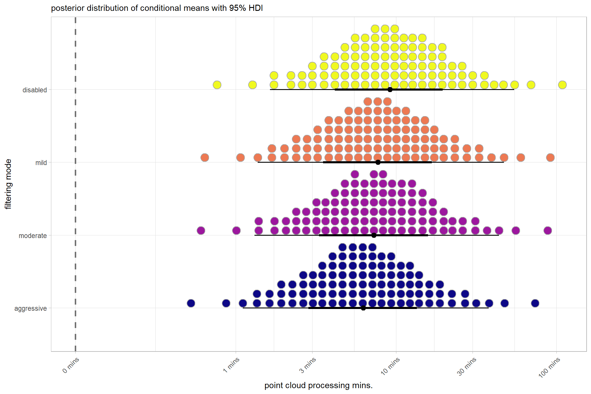
let’s compare these results to the results from our one nominal predictor model above and two nominal predictor model without site effects above and two nominal predictor model with site effects above
ptime_data %>%
  dplyr::distinct(depth_maps_generation_filtering_mode) %>%
  tidybayes::add_epred_draws(
    brms4_mod
    # this part is crucial
    , re_formula = ~ (1 | depth_maps_generation_filtering_mode)
  ) %>%
  dplyr::mutate(value = .epred, src = "site+two nominal predictor: gamma") %>%
  dplyr::bind_rows(
    ptime_data %>%
      dplyr::distinct(depth_maps_generation_filtering_mode) %>%
      tidybayes::add_epred_draws(
        brms3_mod
        # this part is crucial
        , re_formula = ~ (1 | depth_maps_generation_filtering_mode)
      ) %>%
      dplyr::mutate(value = .epred, src = "site+two nominal predictor: gauss")
    , ptime_data %>%
      dplyr::distinct(depth_maps_generation_filtering_mode) %>%
      tidybayes::add_epred_draws(
        brms2_mod
        # this part is crucial
        , re_formula = ~ (1 | depth_maps_generation_filtering_mode)
      ) %>%
      dplyr::mutate(value = .epred, src = "two nominal predictor")
  ) %>%
  ggplot(mapping = aes(y = src, x = value, color = src, group = src)) +
  geom_vline(xintercept = 0, linetype = "dashed", color = "gray44") +
  tidybayes::stat_pointinterval(position = "dodge") +
  facet_grid(rows = vars(depth_maps_generation_filtering_mode), switch = "y") +
  scale_y_discrete(NULL, breaks = NULL) +
  scale_x_continuous(breaks = scales::extended_breaks(10)) +
  scale_color_manual(values = viridis::turbo(n = 4, begin = 0.2, end = 0.8)[c(2:4)]) +
  labs(
    y = "", x = "point cloud processing mins."
    , color = "model"
  ) +
  theme_light() +
  theme(
    legend.position = "top", strip.text = element_text(color = "black", face = "bold")
  ) +
  guides(
    color = guide_legend(
      nrow = 2, byrow = T
      , override.aes = list(shape = 15, size = 10, lwd = NA)
    )
  )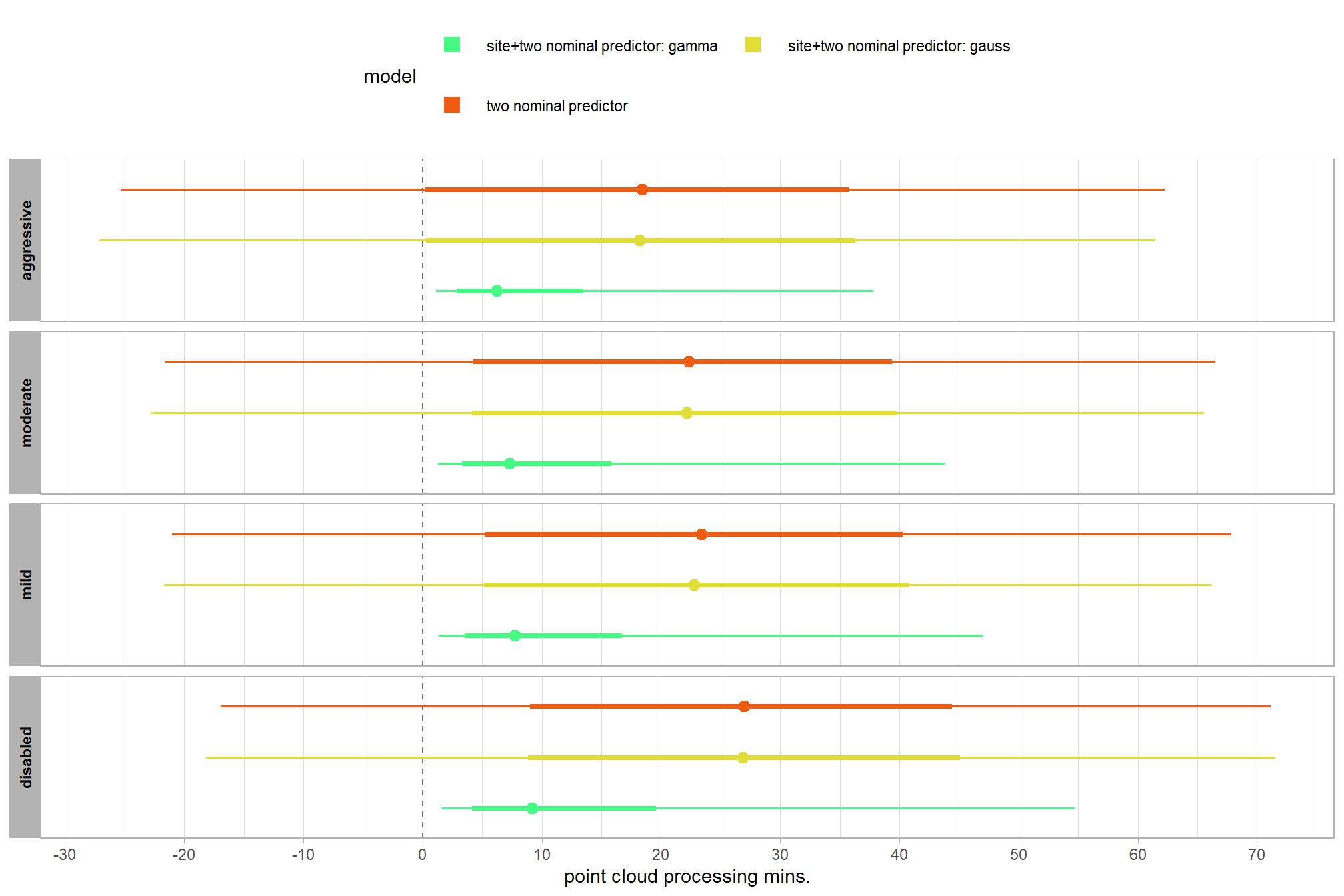
Finally, we can quantify the variation in processing time by comparing the \(\sigma\) posteriors.
# extract the posterior draws
brms::as_draws_df(brms4_mod) %>%
  dplyr::select(c(shape,tidyselect::starts_with("sd_"))) %>%
  tidyr::pivot_longer(dplyr::everything()) %>%
  # dplyr::group_by(name) %>%
  # tidybayes::median_hdi(value) %>%
  dplyr::mutate(
    name = name %>%
      stringr::str_replace_all("depth_maps_generation_quality", "quality") %>%
      stringr::str_replace_all("depth_maps_generation_filtering_mode", "filtering") %>%
      forcats::fct_reorder(value)
  ) %>%
# plot
  ggplot(aes(x = value, y = name)) +
  tidybayes::stat_dotsinterval(
    point_interval = median_hdi, .width = .95
    , justification = -0.04
    , shape = 21 #, point_size = 3
    , quantiles = 100
  ) +
  labs(x = "", y = "") +
  theme_light()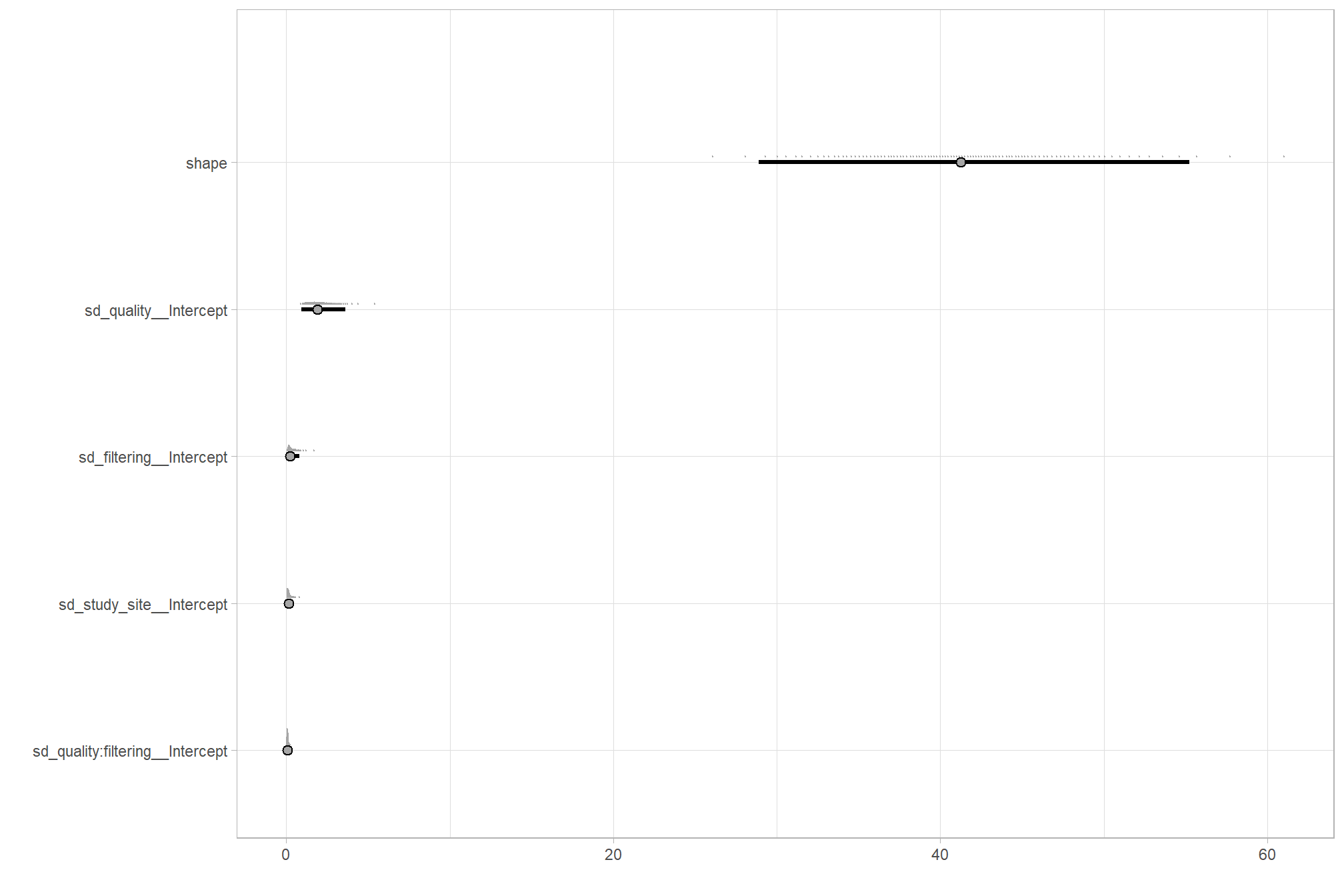
and perform model selection via information criteria with the brms::loo_compare() function
brms4_mod = brms::add_criterion(brms4_mod, criterion = c("loo", "waic"))
brms::loo_compare(brms1_mod, brms2_mod, brms3_mod, brms4_mod, criterion = "loo")
## elpd_diff se_diff
## brms4_mod 0.0 0.0
## brms3_mod -210.3 17.0
## brms2_mod -216.9 16.9
## brms1_mod -233.3 18.7