The cloud2trees package offers compiled processing routines for generating individual-tree forest inventories directly from aerial point cloud data. Designed to integrate easily into existing silviculture and fire management workflows, the package streamlines complex processing steps that are often fragmented across multiple software tools.
This demonstration provides a broad overview of cloud2trees by walking through the entire process, starting with an overview of point cloud data, progressing the data through the core tree detection and metric extraction pipeline, and concluding with visualization and aggregation of the final outputs. The goal is to illustrate how the package quickly transforms raw 3D data into actionable, attributable, and spatially explicit tree lists ready for further analysis or planning and modeling applications.
Let’s load the libraries we’ll use
Raw Point Cloud Data
We’ll start with a quick overview of aerial point cloud data and its
typical processing in R, independent of the cloud2trees package. Aerial
point cloud data are highly detailed 3D datasets that capture the
forest’s structure. This data is typically acquired via fixed wing
crewed aircraft or uncrewed aerial systems (UAS) equipped with lidar
sensors or high-resolution cameras for Digital Aerial Photogrammetry
(DAP). We will demonstrate basic handling using the widely adopted
lidR package, including initial file loading
(.las/.laz), metadata review, and essential 3D
visualization. See the lidR book by point cloud
processing expert Jean-Romain
Roussel for excellent detail on data processing with this
foundational package.
While lidR provides the necessary foundational tools for
these tasks, cloud2trees steps in to fill the crucial gap by compiling
and automating the more complex, sequential processing steps, including
built-in handling for large extent data that can be challenging for
users scripting a pipeline from scratch.
Let’s load the data for the tutorial which is a small data set that
ships with the lidR package
# the path to a single .las file
las_fpath <- system.file(package = "lidR", "extdata", "MixedConifer.laz")
# load the single file point cloud with lidR selecting only the primary information
las_data <- lidR::readLAS(las_fpath, select = "xyzic")
what is this data?
las_data
#> class        : LAS (v1.2 format 1)
#> memory       : 1.1 Mb
#> extent       : 481260, 481350, 3812921, 3813011 (xmin, xmax, ymin, ymax)
#> coord. ref.  : NAD83 / UTM zone 12N
#> area         : 8072 m²
#> points       : 37.7 thousand points
#> type         : airborne
#> density      : 4.67 points/m²
that is very useful information and we can explore the actual data of the point cloud to get more detail
las_data@data %>% dplyr::glimpse()
#> Rows: 37,657
#> Columns: 5
#> $ X              <dbl> 481349.5, 481348.7, 481348.7, 481348.6, 481348.6, 48134…
#> $ Y              <dbl> 3813011, 3813011, 3813010, 3813009, 3813011, 3813011, 3…
#> $ Z              <dbl> 0.07, 0.11, 0.04, 0.02, 0.04, 0.03, 0.10, 0.15, 7.40, 0…
#> $ Intensity      <int> 132, 202, 148, 155, 178, 138, 126, 157, 125, 133, 131, …
#> $ Classification <int> 1, 2, 2, 1, 2, 2, 2, 1, 1, 2, 2, 1, 1, 2, 1, 1, 2, 2, 1…
we can explore the X, Y, and Z data further
las_data@data %>% dplyr::select(X,Y,Z) %>% summary()
#>        X                Y                 Z
#>  Min.   :481260   Min.   :3812921   Min.   : 0.00
#>  1st Qu.:481283   1st Qu.:3812944   1st Qu.: 1.81
#>  Median :481305   Median :3812966   Median :14.08
#>  Mean   :481305   Mean   :3812966   Mean   :12.01
#>  3rd Qu.:481328   3rd Qu.:3812989   3rd Qu.:18.67
#>  Max.   :481350   Max.   :3813011   Max.   :32.07
because this is a relatively small data set, we can visualize the 3D data with the points colored by the Z measurement
lidR::plot(
  x = las_data
  , color = "Z", bg = "white"
  , legend = T
  , pal = grDevices::heat.colors(55)
  , rgl = T
)
rgl::rglwidget()
now that we’ve covered the foundational concepts of point cloud data,
we’re ready to put our cloud2trees pipeline into action using the core
cloud2trees() function to rapidly generate a complete
forest inventory.
Core cloud2trees() Pipeline
The heart of the package is the cloud2trees() function,
which runs the entire Individual Tree Detection (ITD) and attribute
extraction workflow based on settings defined by the user. To illustrate
its immediate simplicity, we will first demonstrate the execution of
this all-in-one pipeline using the default settings, specifying just the
input location of the example point cloud and where we want to save the
results (a temporary directory for this example). While we strongly
recommend that users customize the function parameters to meet their
specific study objectives, this demonstration will illustrate how simply
cloud2trees can process raw point cloud data to produce a spatial forest
inventory tree list as well as intermediate products like the Digital
Terrain Model (DTM) and Canopy Height Model (CHM).
cloud2trees_ans <- cloud2trees::cloud2trees(
  input_las_dir = las_fpath
  , output_dir = tempdir()
)
That single cloud2trees() function call is all that is
needed to produce a spatial forest inventory tree list, DTM, and CHM
from raw point cloud data
Reviewing Outputs
Regardless of the custom parameters selected by the user, upon
successful completion over an area with trees, the
cloud2trees() function will always return a spatial forest
inventory tree list (including core attributes such as height, location,
and crown area as is typical of ITD processing), as well as the
intermediate DTM and CHM rasters. This section focuses on reviewing
these results, visualizing the segmented crowns and tree tops.
Let’s check out what is included in the return from the
cloud2trees() function.
# what is it?
cloud2trees_ans %>% names()
#> [1] "crowns_sf"       "treetops_sf"     "dtm_rast"        "chm_rast"
#> [5] "foresttype_rast"
There is a digital terrain model (DTM) raster
# there's a DTM
cloud2trees_ans$dtm_rast
#> class       : SpatRaster
#> size        : 90, 90, 1  (nrow, ncol, nlyr)
#> resolution  : 1, 1  (x, y)
#> extent      : 481260, 481350, 3812921, 3813011  (xmin, xmax, ymin, ymax)
#> coord. ref. : NAD83 / UTM zone 12N (EPSG:26912)
#> source      : dtm_1m.tif
#> name        : 1_dtm_1m
#> min value   : 0.000000
#> max value   : 0.622001
The DTM was created at the cloud2trees() default 1 m
resolution and that the elevations vary between 0.00 and 0.62 m.
we can plot the DTM using terra::plot()
terra::plot(cloud2trees_ans$dtm_rast)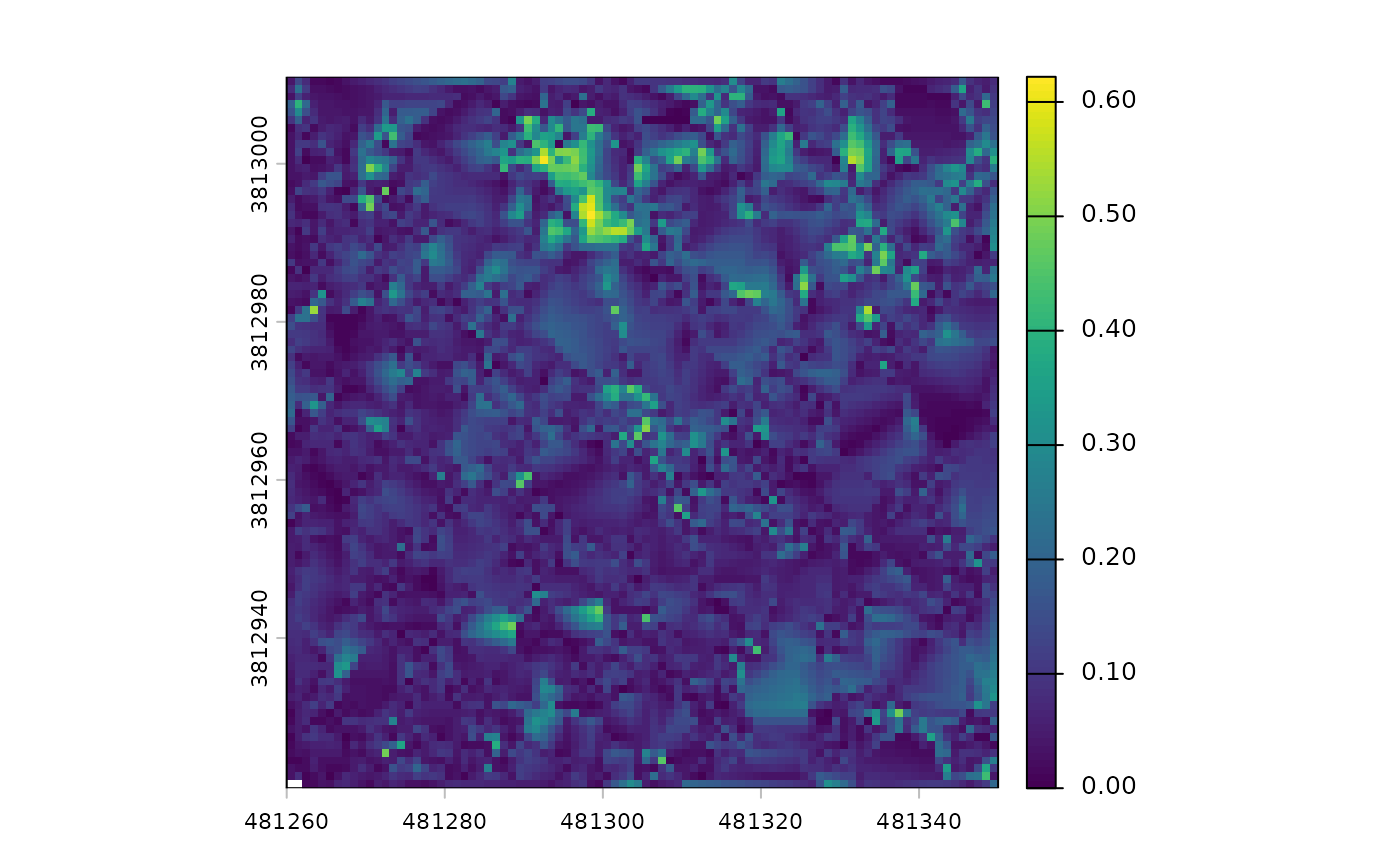
While the plot shows a fair amount of variation, let’s remember it only represents 0.62 m of vertical relief. If we looked at an area with 60 m of vertical relief, for example, we would not even notice these small fluctuations.
There is a canopy height model (CHM) raster
# there's a CHM
cloud2trees_ans$chm_rast
#> class       : SpatRaster
#> size        : 360, 360, 1  (nrow, ncol, nlyr)
#> resolution  : 0.25, 0.25  (x, y)
#> extent      : 481260, 481350, 3812921, 3813011  (xmin, xmax, ymin, ymax)
#> coord. ref. : NAD83 / UTM zone 12N (EPSG:26912)
#> source      : chm_0.25m.tif
#> name        :   chm
#> min value   :  2.01
#> max value   : 32.02
The CHM was created at the cloud2trees() default 0.25 m
resolution and that the elevations vary between 2.01 and 32.02 m.
we can plot the CHM using terra::plot()
terra::plot(cloud2trees_ans$chm_rast, col = grDevices::heat.colors(55, alpha = 0.88))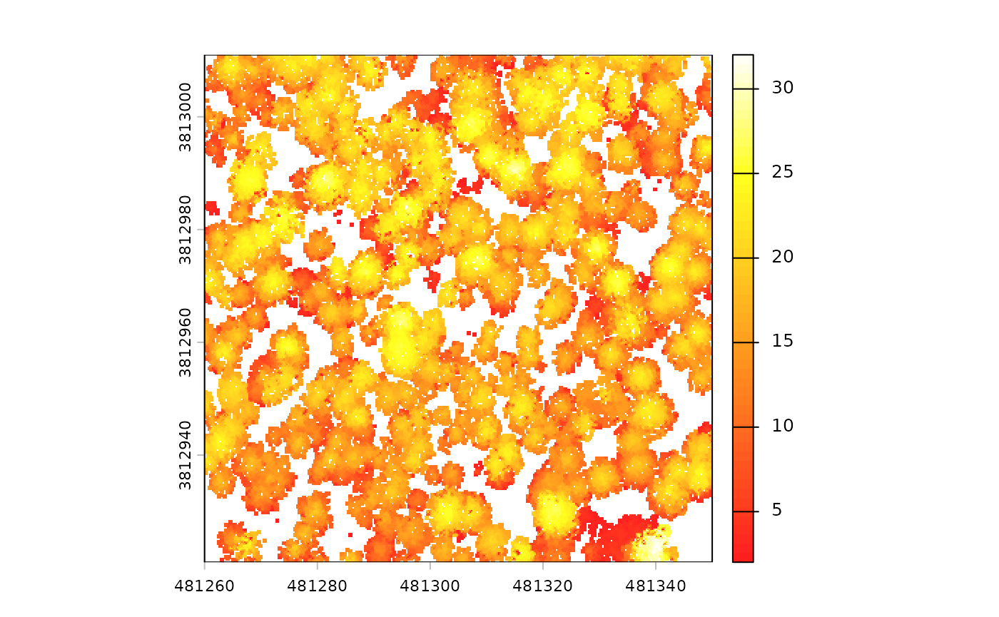
the treetops_sf object in the return from
cloud2trees() is a spatial data frame representing the
extracted tree tops as individual points
cloud2trees_ans$treetops_sf %>% dplyr::glimpse()
#> Rows: 346
#> Columns: 25
#> $ treeID                    <chr> "1_481294.4_3813010.9", "2_481312.9_3813010.…
#> $ tree_height_m             <dbl> 15.85, 13.44, 22.07, 22.48, 22.92, 24.41, 22…
#> $ crown_area_m2             <dbl> 10.0625, 6.2500, 6.1875, 11.3125, 17.0000, 1…
#> $ fia_est_dbh_cm            <dbl> NA, NA, NA, NA, NA, NA, NA, NA, NA, NA, NA, …
#> $ fia_est_dbh_cm_lower      <dbl> NA, NA, NA, NA, NA, NA, NA, NA, NA, NA, NA, …
#> $ fia_est_dbh_cm_upper      <dbl> NA, NA, NA, NA, NA, NA, NA, NA, NA, NA, NA, …
#> $ dbh_cm                    <dbl> NA, NA, NA, NA, NA, NA, NA, NA, NA, NA, NA, …
#> $ is_training_data          <lgl> NA, NA, NA, NA, NA, NA, NA, NA, NA, NA, NA, …
#> $ dbh_m                     <dbl> NA, NA, NA, NA, NA, NA, NA, NA, NA, NA, NA, …
#> $ radius_m                  <dbl> NA, NA, NA, NA, NA, NA, NA, NA, NA, NA, NA, …
#> $ basal_area_m2             <dbl> NA, NA, NA, NA, NA, NA, NA, NA, NA, NA, NA, …
#> $ basal_area_ft2            <dbl> NA, NA, NA, NA, NA, NA, NA, NA, NA, NA, NA, …
#> $ ptcld_extracted_dbh_cm    <dbl> NA, NA, NA, NA, NA, NA, NA, NA, NA, NA, NA, …
#> $ ptcld_predicted_dbh_cm    <dbl> NA, NA, NA, NA, NA, NA, NA, NA, NA, NA, NA, …
#> $ tree_cbh_m                <dbl> NA, NA, NA, NA, NA, NA, NA, NA, NA, NA, NA, …
#> $ is_training_cbh           <lgl> NA, NA, NA, NA, NA, NA, NA, NA, NA, NA, NA, …
#> $ forest_type_group_code    <chr> NA, NA, NA, NA, NA, NA, NA, NA, NA, NA, NA, …
#> $ forest_type_group         <chr> NA, NA, NA, NA, NA, NA, NA, NA, NA, NA, NA, …
#> $ hardwood_softwood         <chr> NA, NA, NA, NA, NA, NA, NA, NA, NA, NA, NA, …
#> $ comp_trees_per_ha         <dbl> NA, NA, NA, NA, NA, NA, NA, NA, NA, NA, NA, …
#> $ comp_relative_tree_height <dbl> NA, NA, NA, NA, NA, NA, NA, NA, NA, NA, NA, …
#> $ comp_dist_to_nearest_m    <dbl> NA, NA, NA, NA, NA, NA, NA, NA, NA, NA, NA, …
#> $ max_crown_diam_height_m   <dbl> NA, NA, NA, NA, NA, NA, NA, NA, NA, NA, NA, …
#> $ is_training_hmd           <lgl> NA, NA, NA, NA, NA, NA, NA, NA, NA, NA, NA, …
#> $ geometry                  <POINT [m]> POINT (481294.4 3813011), POINT (48131…
The tree list contains 346 rows and 25 columns. The 346 rows means
that cloud2trees() detected 346 trees across this 0.81
hectare area. The default use of cloud2trees() provides the
height, crown area, and location (X and Y coordinate) for each of the
trees it identified. However, we also see there are many columns with
NA values and we will explore how cloud2trees can estimate
these attributes in later tutorials.
the crowns_sf object in the return from
cloud2trees() is a spatial data frame representing the
extracted tree crowns as polygons
cloud2trees_ans$crowns_sf %>% dplyr::glimpse()
#> Rows: 346
#> Columns: 27
#> $ treeID                    <chr> "1_481294.4_3813010.9", "2_481312.9_3813010.…
#> $ tree_height_m             <dbl> 15.85, 13.44, 22.07, 22.48, 22.92, 24.41, 22…
#> $ tree_x                    <dbl> 481294.4, 481312.9, 481325.1, 481333.4, 4813…
#> $ tree_y                    <dbl> 3813011, 3813011, 3813011, 3813011, 3813011,…
#> $ crown_area_m2             <dbl> 10.0625, 6.2500, 6.1875, 11.3125, 17.0000, 1…
#> $ geometry                  <GEOMETRY [m]> POLYGON ((481292.5 3813011,..., POL…
#> $ fia_est_dbh_cm            <dbl> NA, NA, NA, NA, NA, NA, NA, NA, NA, NA, NA, …
#> $ fia_est_dbh_cm_lower      <dbl> NA, NA, NA, NA, NA, NA, NA, NA, NA, NA, NA, …
#> $ fia_est_dbh_cm_upper      <dbl> NA, NA, NA, NA, NA, NA, NA, NA, NA, NA, NA, …
#> $ dbh_cm                    <dbl> NA, NA, NA, NA, NA, NA, NA, NA, NA, NA, NA, …
#> $ is_training_data          <lgl> NA, NA, NA, NA, NA, NA, NA, NA, NA, NA, NA, …
#> $ dbh_m                     <dbl> NA, NA, NA, NA, NA, NA, NA, NA, NA, NA, NA, …
#> $ radius_m                  <dbl> NA, NA, NA, NA, NA, NA, NA, NA, NA, NA, NA, …
#> $ basal_area_m2             <dbl> NA, NA, NA, NA, NA, NA, NA, NA, NA, NA, NA, …
#> $ basal_area_ft2            <dbl> NA, NA, NA, NA, NA, NA, NA, NA, NA, NA, NA, …
#> $ ptcld_extracted_dbh_cm    <dbl> NA, NA, NA, NA, NA, NA, NA, NA, NA, NA, NA, …
#> $ ptcld_predicted_dbh_cm    <dbl> NA, NA, NA, NA, NA, NA, NA, NA, NA, NA, NA, …
#> $ tree_cbh_m                <dbl> NA, NA, NA, NA, NA, NA, NA, NA, NA, NA, NA, …
#> $ is_training_cbh           <lgl> NA, NA, NA, NA, NA, NA, NA, NA, NA, NA, NA, …
#> $ forest_type_group_code    <chr> NA, NA, NA, NA, NA, NA, NA, NA, NA, NA, NA, …
#> $ forest_type_group         <chr> NA, NA, NA, NA, NA, NA, NA, NA, NA, NA, NA, …
#> $ hardwood_softwood         <chr> NA, NA, NA, NA, NA, NA, NA, NA, NA, NA, NA, …
#> $ comp_trees_per_ha         <dbl> NA, NA, NA, NA, NA, NA, NA, NA, NA, NA, NA, …
#> $ comp_relative_tree_height <dbl> NA, NA, NA, NA, NA, NA, NA, NA, NA, NA, NA, …
#> $ comp_dist_to_nearest_m    <dbl> NA, NA, NA, NA, NA, NA, NA, NA, NA, NA, NA, …
#> $ max_crown_diam_height_m   <dbl> NA, NA, NA, NA, NA, NA, NA, NA, NA, NA, NA, …
#> $ is_training_hmd           <lgl> NA, NA, NA, NA, NA, NA, NA, NA, NA, NA, NA, …
Notice that cloud2trees_ans$crowns_sf and
cloud2trees_ans$treetops_sf have the exact same
structure but one is spatial polygons and the other is spatial
points.
Now let’s create a visual of the individual tree crowns stored in the
crowns_sf object overlaid on the CHM. This time, we’ll plot
using the ggplot2 package
cloud2trees_ans$chm_rast %>%
  terra::as.data.frame(xy = T) %>%
  dplyr::rename(f = 3) %>%
  ggplot2::ggplot() +
  ggplot2::geom_tile(
    mapping = ggplot2::aes(x = x, y = y, fill = f)
    ) +
  ggplot2::geom_sf(
    data = cloud2trees_ans$crowns_sf
    , color = "grey33"
    , lwd = 0.8
    ) +
  ggplot2::scale_fill_gradientn(colors = grDevices::heat.colors(55, alpha = 0.88)) +
  ggplot2::labs(fill = "CHM (m)") +
  ggplot2::theme_void()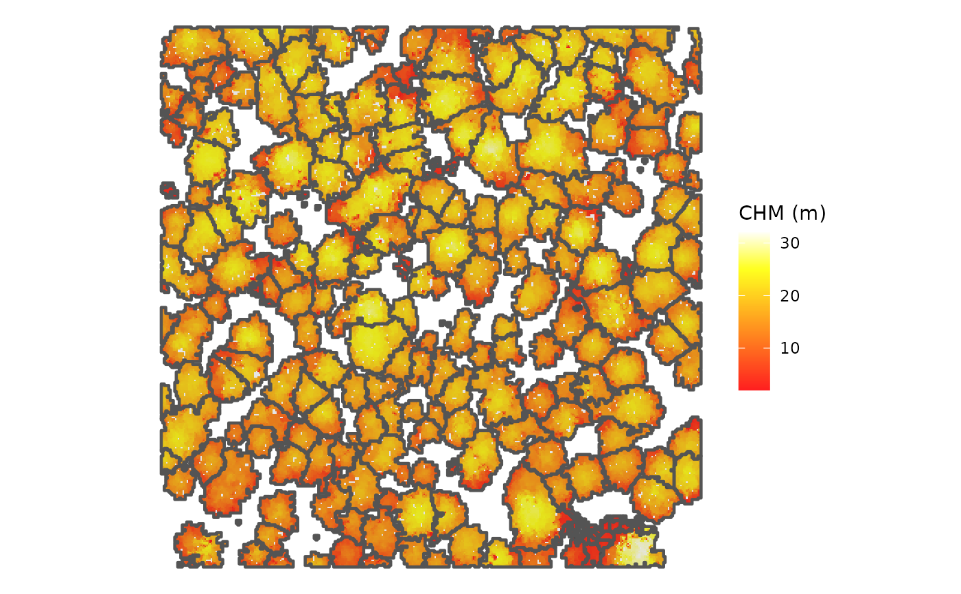
This figure displays the individual tree crowns that
cloud2trees() identified using its default variable window
function for tree detection (i.e. the ws argument). If you
look closely, you can likely find places where tree crowns are being
over or under divided. In a later tutorial we will look at how the
itd_tuning() function of cloud2trees can be used to
optimize local tree detection given the crown architecture of the forest
being analyzed.
Analyzing Outputs
The ultimate goal of cloud2trees is to provide accurate and spatially
explicit inputs that directly support management decisions. This final
section demonstrates how the output spatial tree list can be immediately
used for forest management and planning. We will showcase examples such
as calculating stand-level metrics (e.g. trees per hectare and mean
stand height), generating height distributions, and identifying
potentially ecologically important trees. This brief overview is meant
to showcase how easily insight can be gained from the
cloud2trees() spatial inventory, improving access to data
and enabling cross-disciplinary integration to spur novel forest
management approaches and enable collaborative action.
Stand-Level Metrics
We’ll pretend our forest stand is the central 4,000 m2 of the point cloud data and create a square polygon to use as our stand boundary
my_stand <-
  cloud2trees_ans$treetops_sf %>%
    sf::st_union() %>%
    sf::st_centroid() %>%
    sf::st_buffer(sqrt(4000)/2, endCapStyle = "SQUARE")
Let’s look the tree top points identified by
cloud2trees() in relation to the stand boundary. We’ll
color the tree top points by tree height
# what is this?
ggplot2::ggplot() +
  # tree tops
  ggplot2::geom_sf(
    data = cloud2trees_ans$treetops_sf
    , mapping = ggplot2::aes(color = tree_height_m)
    , size = 1.8
  ) +
  # stand polygon
  ggplot2::geom_sf(
    data = my_stand
    , fill = NA, color = "black", lwd = 1.1
  ) +
  ggplot2::scale_color_distiller(
    palette = "Blues", direction = 1, name = "tree ht. (m)"
  ) +
  ggplot2::theme_void()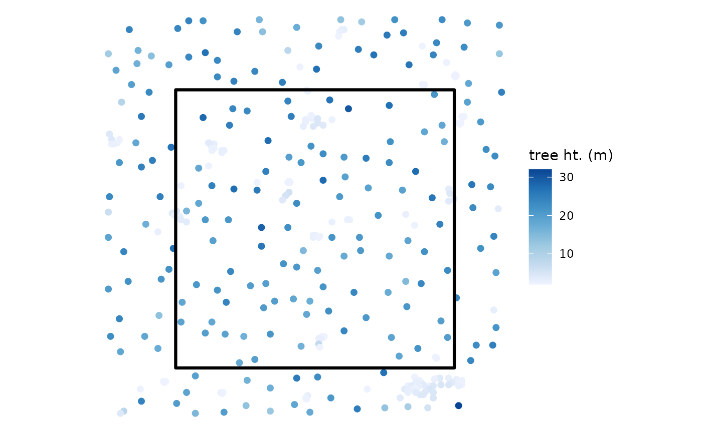
to get stand-level metrics we can crop our tree list to the stand
boundary and summarize. we’ll do this all in one tidy pipeline but you
can break the pipes (%>%) to see what each step
does.
# first we'll crop the tree list to the stand
treetops_in_stand <- cloud2trees_ans$treetops_sf %>% sf::st_intersection(my_stand)
# summarize
stand_summary <-
  treetops_in_stand %>%
  sf::st_drop_geometry() %>% # don't need geom now
  # summarize
  dplyr::summarise(
    mean_tree_height_m = mean(tree_height_m)
    , n_trees = dplyr::n()
  ) %>%
  # add stand information
  dplyr::mutate(
    stand_area_m2 = sf::st_area(my_stand) %>% as.numeric()
    , stand_area_ha = stand_area_m2/10000
    , trees_per_ha = n_trees/stand_area_ha
  )
# what is this?
stand_summary
#> # A tibble: 1 × 5
#>   mean_tree_height_m n_trees stand_area_m2 stand_area_ha trees_per_ha
#>                <dbl>   <int>         <dbl>         <dbl>        <dbl>
#> 1               13.9     158         4000.         0.400         395.
cloud2trees() identified 158 trees in the 0.40 ha stand
resulting in 395.0 trees per hectare (TPH). Based on these 158 trees,
the mean stand height is 13.9 m.
Height Distributions
We’ll continue to look at the trees within our stand to explore the tree height distribution.
A simple density plot of heights can be generated quickly
treetops_in_stand %>%
  ggplot2::ggplot() +
  ggplot2::geom_density(
    ggplot2::aes(x = tree_height_m)
    , alpha = 0.88
    , fill = "navy", color = NA
  ) +
  ggplot2::labs(x = "tree ht. (m)") +
  ggplot2::theme_light()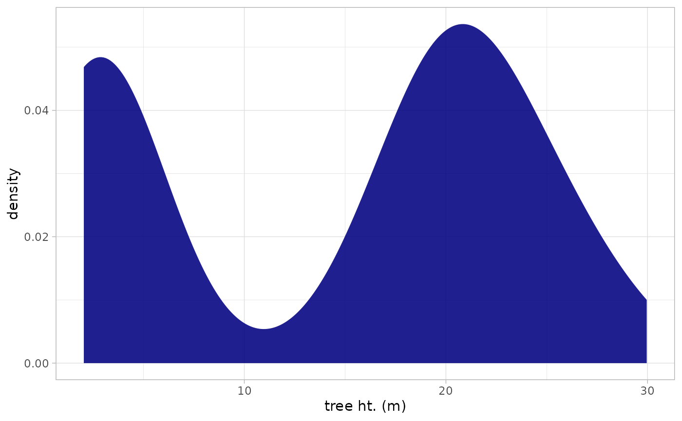
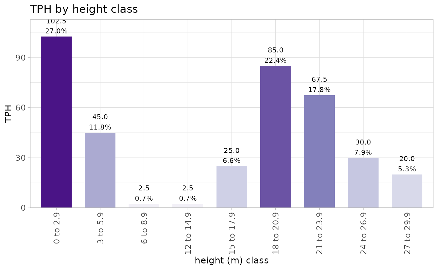
we can also create custom height bins and summarize the trees within
those bins. again, this is one big tidy pipeline but you can break the
pipes (%>%) to see what each step does.
treetops_in_stand %>%
  sf::st_drop_geometry() %>%
  dplyr::mutate(
    height_bin = ggplot2::cut_width(
      tree_height_m, width = 3, boundary = 0, closed = "left"
    )
  ) %>%
  dplyr::group_by(height_bin) %>%
  dplyr::summarise(
    n_trees = dplyr::n()
  ) %>%
  dplyr::ungroup() %>%
  dplyr::mutate(
    stand_area_m2 = sf::st_area(my_stand) %>% as.numeric()
    , stand_area_ha = stand_area_m2/10000
    , trees_per_ha = n_trees/stand_area_ha
    , tot_trees_per_ha = sum(trees_per_ha)
    , pct = trees_per_ha/tot_trees_per_ha
    , height_bin_lab = paste0(
      stringr::word(
          height_bin
          , 1
          , sep = stringr::fixed(",")
        ) %>% readr::parse_number()
      , " to "
      , stringr::word(
          height_bin
          , -1
          , sep = stringr::fixed(",")
        ) %>% readr::parse_number() %>% `-`(0.1)
    ) %>%
    factor() %>%
    forcats::fct_reorder(
      stringr::word(
        height_bin
        , 1
        , sep = stringr::fixed(",")
      ) %>% readr::parse_number()
    )
  ) %>%
  # plot
  ggplot2::ggplot(
    mapping = ggplot2::aes(
      x = height_bin_lab, y = trees_per_ha
      , fill = trees_per_ha
      , label = paste0(
        scales::comma(trees_per_ha, accuracy = 0.1)
        , "\n"
        , scales::percent(pct, accuracy = 0.1)
      )
    )
  ) +
  ggplot2::geom_col(width = 0.7) +
  ggplot2::geom_text(color = "black", size = 3, vjust = -0.2) +
  ggplot2::scale_fill_distiller(palette = "Purples", direction = 1) +
  ggplot2::scale_y_continuous(
    labels = scales::comma_format(accuracy = 1)
    , expand = ggplot2::expansion(mult = c(0, 0.1))
  ) +
  ggplot2::labs(
    x = "height (m) class"
    , y = "TPH"
    , title = "TPH by height class"
  ) +
  ggplot2::theme_light() +
  ggplot2::theme(
    legend.position = "none"
    , axis.text.y = ggplot2::element_text(size = 10)
    , axis.text.x = element_text(angle = 90, size = 10, vjust = 0.5, hjust = 1)
  )
Identify Potentially Ecologically important trees
finally, let’s identify potentially ecologically important trees based on a height threshold of 24 m across the entire extent of the point cloud data
cloud2trees_ans$treetops_sf %>%
  dplyr::mutate(
    tall_tree = ifelse(tree_height_m>=24,"Tall Tree", "Other")
  ) %>%
  ggplot2::ggplot() +
  # tree tops
  ggplot2::geom_sf(
    mapping = ggplot2::aes(color = tall_tree)
    , size = 1.8
  ) +
  # stand polygon
  ggplot2::geom_sf(
    data = my_stand
    , fill = NA, color = "black", lwd = 1.1
  ) +
  ggplot2::scale_color_viridis_d(option = "viridis", direction = -1, name = "") +
  ggplot2::theme_void() +
  ggplot2::theme(legend.position = "top") +
  ggplot2::guides(color = ggplot2::guide_legend(override.aes = list(size = 5)))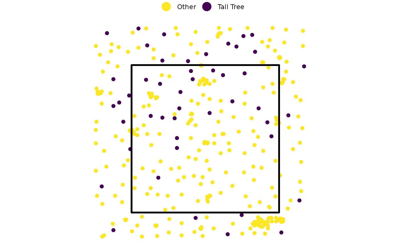
since we have the X and Y coordinates of all trees, we can easily load them onto a tablet or GPS device to navigate to those important trees in the field