Creating DTM and CHM rasters

The cloud2trees package was designed so that complex point cloud processing could be run progressively, allowing users to achieve specific tasks in the overall workflow of generating tree-level forest inventory attributes. The first critical task in this process is generating the foundational raster products: the Digital Terrain Model (DTM) and the Canopy Height Model (CHM), which are considered first-order derivatives coming directly from the point cloud. This tutorial focuses on the dedicated cloud2raster() function, which efficiently packages all the essential, customizable steps for surface generation. For users seeking end-to-end processing, these same parameters are also accessible through the main cloud2trees() function which is demonstrated here.

The cloud2raster() function executes a defined sequence of operations, beginning with tiling the point cloud to manage memory (if necessary). This is followed by sequential operations, including ground classification and outlier removal, leading to DTM creation via ground point triangulation and rasterization. Height normalization of the point cloud and subsequent creation of the CHM based on the highest point per pixel. The process concludes with pit and spike filling and smoothing of the final raster. Understanding and customizing these parameters grants fine-grained influence over surface generation, with the CHM directly influencing the reliability of subsequent Individual Tree Detection (ITD) steps.

Let’s load the libraries we’ll use

library(cloud2trees)
library(ggplot2)
library(magrittr)
library(terra)
library(sf)
library(patchwork)

Extract raster data from point cloud: Defaults

We’ll begin by using a small point cloud dataset that ships with the lidR package for processing (we previously used this data in the package overview demonstration. The cloud2raster() function requires the input_las_dir argument to be the path to a single point cloud file (.las or .laz) or a directory containing these files. If a directory is utilized, the function treats the directory and all sub-directories as a single point cloud catalog, processing all contained files together. Therefore, ensure that the specified directory contains only the point cloud data intended for a single processing area, as the function recursively processes all files within its path.

We also need to define where outputs should be written in the output_dir argument. For demonstration we’ll use a temporary directory but you’ll likely want to point to a permanent directory, for example: C:/Data/MixedConifer.

# the path to a single .las|.laz file 
#  -or- the directory to a folder with many .las|.laz files
las_dir <- system.file(package = "lidR", "extdata", "MixedConifer.laz")
# output directroy
out_dir <- tempdir()

First, we’ll run cloud2raster() with all of the default settings

cloud2raster_ans <- cloud2trees::cloud2raster(
  input_las_dir = las_dir
  , output_dir = out_dir
)

You will see a progress bar giving updates about what the process is doing.

Now, let’s explore what cloud2raster() created

cloud2raster_ans %>% names()
#> [1] "dtm_rast"                     "chm_rast"                    
#> [3] "create_project_structure_ans" "chunk_las_catalog_ans"       
#> [5] "normalize_flist"

The above command should show you a list of five objects that the output contains. The dtm_rast and chm_rast contain the main raster outputs, but some users might care about the other three objects. The normalize_flist contains a list of the height normalized point cloud tiles, chunk_las_catalog_ans is a ggplot object for creating a plot that displays the dataset’s tiles, and the create_project_structure_ans is a table listing all of the data source locations and output file locations.

cloud2raster() also wrote data to the disk at the location defined in the output_dir argument for use outside of the current working session. The process creates a sub-folder containing the outputs which is always titled point_cloud_processing_delivery. If you run this process multiple times using the same output_dir location, then everything in the point_cloud_processing_delivery directory will be overwritten. As such, if you intend to perform multiple iterations of the processing in the same output_dir location it is recommended you rename the point_cloud_processing_delivery directory before running the next iteration.

Let’s see what was written to the disk.

file.path(out_dir, "point_cloud_processing_delivery") %>% 
  list.files()
#> [1] "chm_0.25m.tif"         "dtm_1m.tif"            "raw_las_ctg_info.gpkg"

There is a .tif file for both the DTM and CHM raster which includes the resolution of the data in the file name.

There is also a raw_las_ctg_info.gpkg file which includes the processing extent covered by the point cloud data as a spatial polygon. This data can be used to ensure the point cloud covered your intended area of interest or to calculate area-based metrics by properly representing the area covered by the data. This spatial extent is the same as the chunk_las_catalog_ans$process_data return from the cloud2raster() function.

file.path(out_dir, "point_cloud_processing_delivery", "raw_las_ctg_info.gpkg") %>% 
  sf::st_read(quiet = T) %>% 
  ggplot2::ggplot() + 
  ggplot2::geom_sf(fill = NA, color = "navy", lwd = 5) +
  ggplot2::geom_sf(
    data = cloud2raster_ans$chunk_las_catalog_ans$process_data
    , fill = NA, color = "gold", lwd = 1.3
  ) +
  ggplot2::theme_light()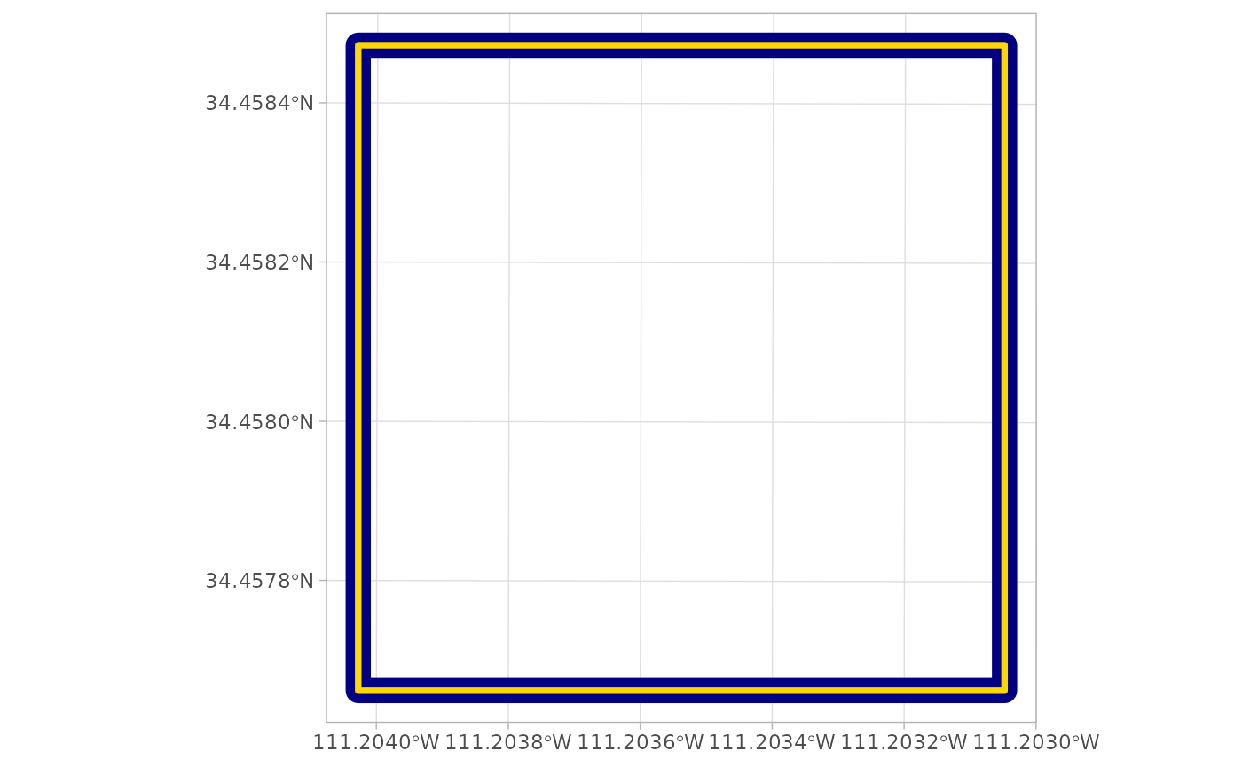

Let’s look at the digital terrain model (DTM) raster

# there's a DTM
cloud2raster_ans$dtm_rast
#> class       : SpatRaster 
#> size        : 90, 90, 1  (nrow, ncol, nlyr)
#> resolution  : 1, 1  (x, y)
#> extent      : 481260, 481350, 3812921, 3813011  (xmin, xmax, ymin, ymax)
#> coord. ref. : NAD83 / UTM zone 12N (EPSG:26912) 
#> source      : dtm_1m.tif 
#> name        : 1_dtm_1m 
#> min value   : 0.000000 
#> max value   : 0.622001

The DTM was created at the cloud2raster() default 1 m resolution and that the elevations vary between 0.00 and 0.62 m.

we can plot the DTM using terra::plot()

terra::plot(cloud2raster_ans$dtm_rast)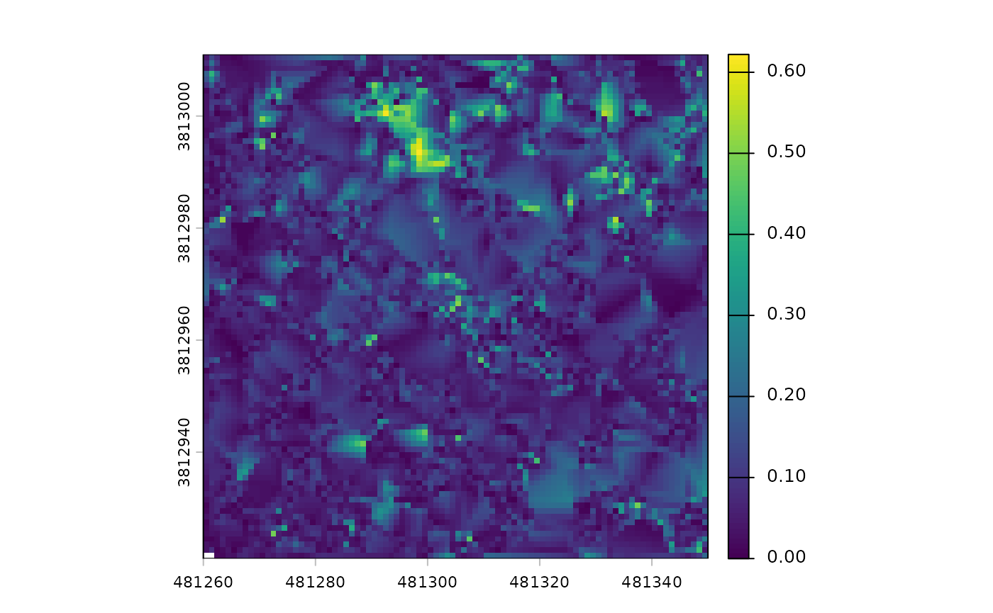

While the plot shows a fair amount of variation, let’s remember it only represents 0.62 m of vertical relief. If we looked at an area with 60 m of vertical relief, for example, we would not even notice these small fluctuations.

There is also a canopy height model (CHM) raster

# there's a CHM
cloud2raster_ans$chm_rast
#> class       : SpatRaster 
#> size        : 360, 360, 1  (nrow, ncol, nlyr)
#> resolution  : 0.25, 0.25  (x, y)
#> extent      : 481260, 481350, 3812921, 3813011  (xmin, xmax, ymin, ymax)
#> coord. ref. : NAD83 / UTM zone 12N (EPSG:26912) 
#> source      : chm_0.25m.tif 
#> name        : focal_mean 
#> min value   :       2.01 
#> max value   :      32.02

The CHM was created at the cloud2raster() default 0.25 m resolution and that the elevations vary between 2.01 and 32.02 m.

we can plot the CHM using terra::plot()

terra::plot(cloud2raster_ans$chm_rast, col = grDevices::heat.colors(55, alpha = 0.88))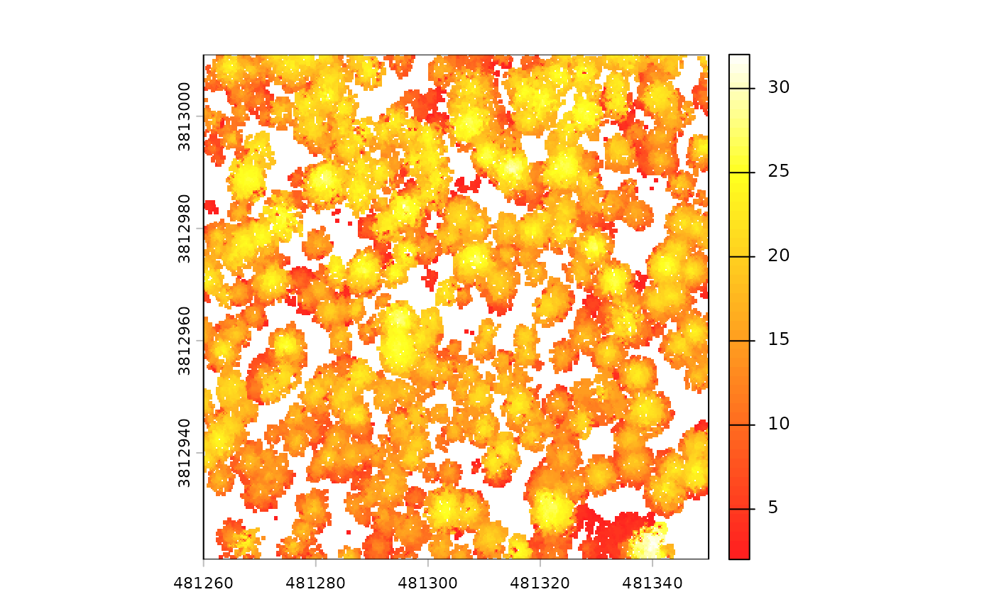

We can also plot this raster data using the ggplot2 package which provides a vast collection of customization for plotting. Here, we’ll use a different color palette than we used with terra::plot() above to demonstrate, but the same grDevices::heat.colors color palette could be used if desired.

cloud2raster_ans$chm_rast %>%
  terra::as.data.frame(xy=T) %>%
  dplyr::rename(f=3) %>%
  ggplot2::ggplot() +
  ggplot2::geom_tile(
    mapping = ggplot2::aes(x=x, y=y, fill=f)
    , alpha = 0.9
  ) +
  ggplot2::scale_fill_viridis_c(option = "plasma") +
  ggplot2::scale_x_continuous(expand = c(0, 0)) +
  ggplot2::scale_y_continuous(expand = c(0, 0)) +
  ggplot2::labs(x = "X", y = "Y", fill = "CHM (m)") +
  ggplot2::theme_light() +
  ggplot2::theme(
    legend.position = "top"
    , axis.text = ggplot2::element_text(size = 7)
  )

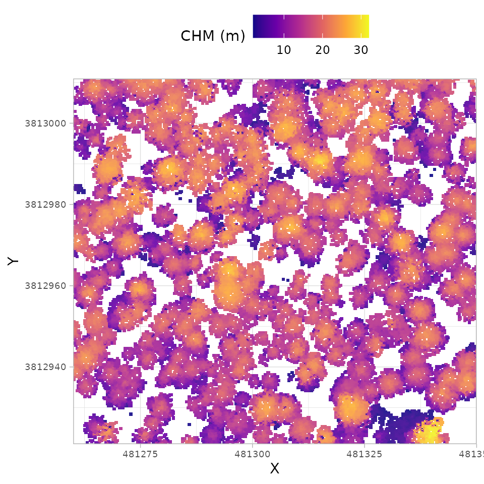
If we really like this figure and want to share it, we can write it out to an image file

ggplot2::ggsave(
  file.path(out_dir,"MixedConifer_chm_025m.jpg")
  , dpi = 300
  , height = 5, width = 6
)

Customizing DTM Generation

The cloud2raster() function offers two key arguments that influence the DTM’s role in the pipeline and the quality of the final raster products. The straightforward argument is dtm_res_m, which controls the final output resolution of the rasterized DTM. The second argument, accuracy_level, requires more context. In processing the point cloud, cloud2raster() always first generates continuous DTM by creating a Delaunay triangulation (or “meshed DTM”) of the ground classified points. This continuous model and the separate rasterized DTM are both generated independent of the accuracy_level setting.

The accuracy_level argument does not affect DTM creation, it determines which DTM product is used to height-normalize the non-ground points for subsequent CHM generation. If accuracy_level is set to ‘1’, the DTM at the resolution defined by the dtm_res_m argument is used for normalization, meaning the chosen dtm_res_m will impact the final CHM quality. However, if accuracy_level is set to ‘2’ or ‘3’, the higher-fidelity triangulated DTM is used for normalization, and the dtm_res_m setting has no impact on the CHM quality. Using higher values (‘2’ or ‘3’) for the accuracy_level argument results in longer processing times, however testing has shown limited differences in the CHM output between level ‘2’ and ‘3’.

We will create DTM at 2 m and 0.5 m resolutions and look at the differences

First, the 2 m DTM

# 2 m dtm
cloud2raster_ans_dtm_2m <- cloud2trees::cloud2raster(
  input_las_dir = las_dir
  , output_dir = out_dir
  , dtm_res_m = 2.0
)

We can confirm that we got the resolution expected by checking the resolution in the X and Y horizontal

# 2 m dtm
paste0(
  "The resolution of `cloud2raster_ans_dtm_2m` is: "
  , paste( terra::res(cloud2raster_ans_dtm_2m$dtm_rast), collapse = "x")
)
#> [1] "The resolution of `cloud2raster_ans_dtm_2m` is: 2x2"

Let’s plot the DTM raster and store it. We won’t show it here as we’ll combine later using patchwork

# plt_dtm_2m
plt_dtm_2m <- cloud2raster_ans_dtm_2m$dtm_rast %>%
  terra::as.data.frame(xy=T) %>%
  dplyr::rename(f=3) %>%
  ggplot2::ggplot() +
  ggplot2::geom_tile(
    mapping = ggplot2::aes(x=x, y=y, fill=f)
    , alpha = 0.9
  ) +
  ggplot2::scale_fill_viridis_c(option = "viridis") +
  ggplot2::scale_x_continuous(expand = c(0, 0)) +
  ggplot2::scale_y_continuous(expand = c(0, 0)) +
  ggplot2::labs(fill = "Elevation (m)", title = "DTM - 2.0 m resolution") +
  ggplot2::theme_light() +
  ggplot2::theme(
    legend.position = "none"
    , axis.text = ggplot2::element_text(size = 5)
    , axis.title = ggplot2::element_blank()
    , plot.title = ggplot2::element_text(hjust = 0.5)
  )

Second, the 0.5 m DTM

# 0.5 m dtm
cloud2raster_ans_dtm_0.5m <- cloud2trees::cloud2raster(
  input_las_dir = las_dir
  , output_dir = out_dir
  , dtm_res_m = 0.5
)

We can confirm that we got the resolution expected by checking the resolution in the X and Y horizontal

# 0.5 m dtm
paste0(
  "The resolution of `cloud2raster_ans_dtm_0.5m` is: "
  , paste( terra::res(cloud2raster_ans_dtm_0.5m$dtm_rast), collapse = "x")
)
#> [1] "The resolution of `cloud2raster_ans_dtm_0.5m` is: 0.5x0.5"

Let’s plot the DTM raster and store it. We won’t show it here as we’ll combine later using patchwork

# plt_dtm_0.5m
plt_dtm_0.5m <- cloud2raster_ans_dtm_0.5m$dtm_rast %>%
  terra::as.data.frame(xy=T) %>%
  dplyr::rename(f=3) %>%
  ggplot2::ggplot() +
  ggplot2::geom_tile(
    mapping = ggplot2::aes(x=x, y=y, fill=f)
    , alpha = 0.9
  ) +
  ggplot2::scale_fill_viridis_c(option = "viridis") +
  ggplot2::scale_x_continuous(expand = c(0, 0)) +
  ggplot2::scale_y_continuous(expand = c(0, 0)) +
  ggplot2::labs(fill = "Elevation (m)", title = "DTM - 0.5 m resolution") +
  ggplot2::theme_light() +
  ggplot2::theme(
    legend.position = "none"
    , axis.text = ggplot2::element_text(size = 5)
    , axis.title = ggplot2::element_blank()
    , plot.title = ggplot2::element_text(hjust = 0.5)
  )

combine with patchwork::wrap_plots()

# patchwork
patchwork::wrap_plots(plt_dtm_2m, plt_dtm_0.5m)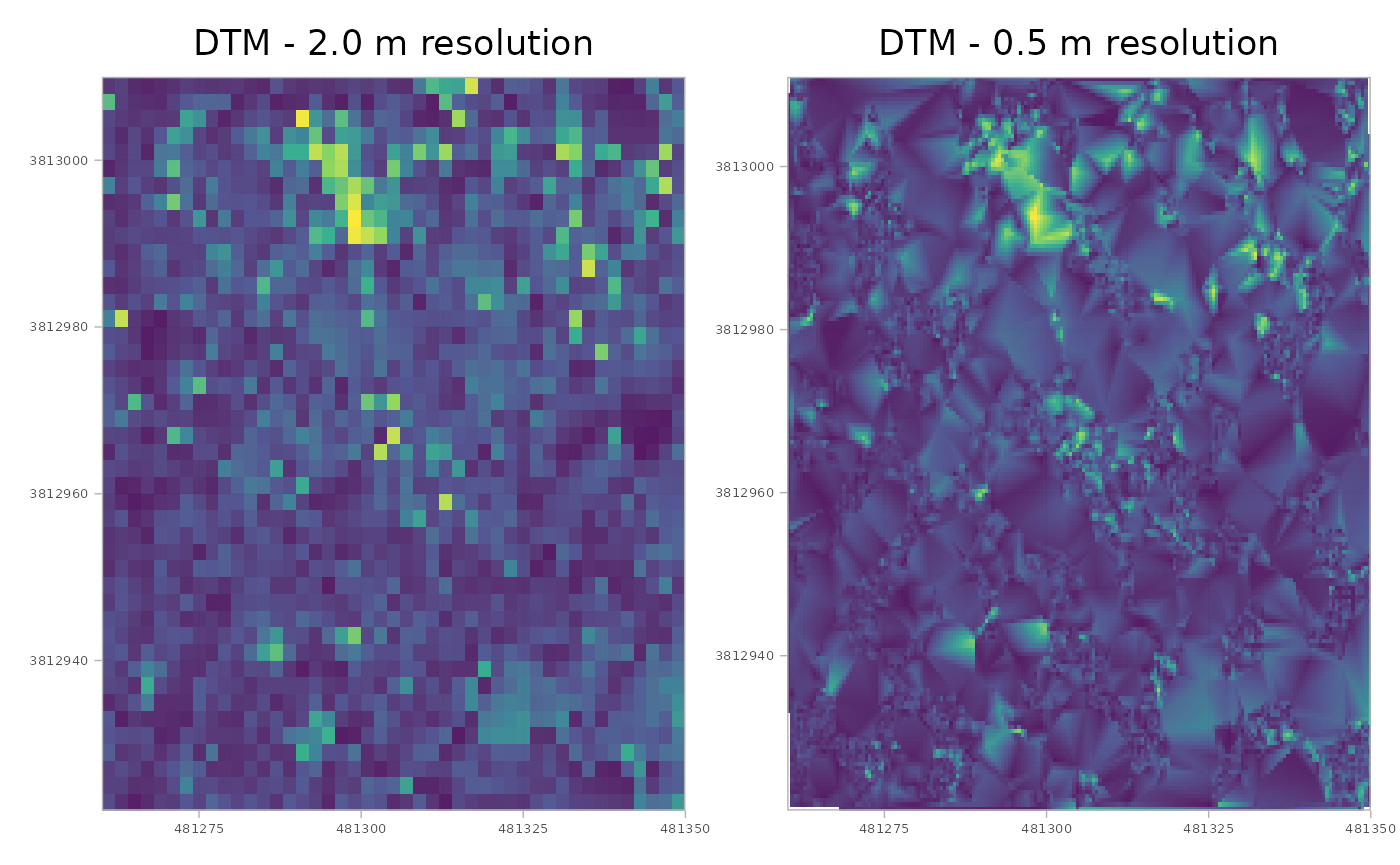

Visually it seems that the 0.5 m resolution has a smoother appearance than the 2.0 m resolution, but it is important to consider the trade-offs as the 0.5 m resolution data contains 16 times as much data.

To maximize flexibility and avoid repeating the computationally expensive point cloud processing (a significant issue, especially for broad-extent data), we strongly advise generating the DTM at the finest resolution needed (i.e. smaller dtm_res_m setting). However, do not set the resolution finer than your analysis requires, as generating and storing unnecessarily high-resolution data wastes both time and disk space. It is far more efficient to later aggregate a fine resolution raster than it is to re-run the entire pipeline. For instance, you can take a fine 0.5 m resolution raster and aggregate it to a more coarse 2.0 m resolution.

Here is how to create a coarser, 2.0 m resolution raster from the 0.5 m resolution raster using terra::aggregate() and we’ll display the resultant resolution in the X and Y horizontal

terra::aggregate(
    cloud2raster_ans_dtm_0.5m$dtm_rast
    , fact = 4
    , fun = "max"
  ) %>% 
  terra::res() %>% 
  paste(collapse = "x")
#> [1] "2x2"

Customizing CHM Generation

Individual Tree Detection (ITD) is traditionally achieved using two main approaches: segmenting trees directly from the point cloud by clustering points based on crown shape and spacing (e.g. Li et al. 2012), or using a Canopy Height Model (CHM) to delineate crowns after identifying tree tops (local maxima; e.g. Popescu and Wynne 2004). The cloud2trees package is built exclusively upon the CHM methodology for ITD. The CHM is therefore the critical, indispensable input for all subsequent steps in our pipeline. Users wishing to explore direct point cloud segmentation methods should consult the functionalities of the lidR package (e.g. lidR::li2012()).

The cloud2raster() function provides several arguments for customization of the CHM. This includes the influence of the previously discussed accuracy_level parameter, which dictates whether the CHM is normalized using the continuous triangulation (level ‘2’ or ‘3’) or the coarser rasterized DTM (level ‘1’). The three primary arguments for customizing the CHM are chm_res_m, which sets the output resolution, and min_height (default 2.0 m) and max_height (default 70 m), which control the height thresholds for CHM cell inclusion. While most high outliers are typically removed during early noise filtering, the max_height parameter primarily serves to limit the height search range to expected forest vegetation heights. The min_height setting, on the other hand, represents the minimum height threshold for any segmented object to be subsequently considered a tree during the ITD process. It is important to note that if the CHM is intended for ITD, these height thresholds must be considered carefully to reflect expected tree heights, but for other uses, the thresholds should be set to meet those specific objectives.

Let’s create CHM data at 0.60 m, 0.40 m, and 0.20 m resolutions and look at the differences. Here, we also demonstrate creating unique folders to store the results from cloud2raster() which would otherwise be written and overwritten to the point_cloud_processing_delivery directory.

# 0.6 m chm
out_dir_0.6m <- file.path(out_dir,"chm_0.6m")
dir.create(out_dir_0.6m)
cloud2raster_ans_chm_0.6m <- cloud2trees::cloud2raster(
  input_las_dir = las_dir
  , output_dir = out_dir_0.6m
  , chm_res_m = 0.6
)
# 0.4 m chm
out_dir_0.4m <- file.path(out_dir,"chm_0.4m")
dir.create(out_dir_0.4m)
cloud2raster_ans_chm_0.4m <- cloud2trees::cloud2raster(
  input_las_dir = las_dir
  , output_dir = out_dir_0.4m
  , chm_res_m = 0.4
)
# 0.2 m chm
out_dir_0.2m <- file.path(out_dir,"chm_0.2m")
dir.create(out_dir_0.2m)
cloud2raster_ans_chm_0.2m <- cloud2trees::cloud2raster(
  input_las_dir = las_dir
  , output_dir = out_dir_0.2m
  , chm_res_m = 0.2
)

We can confirm that we got the resolution expected by checking the resolution in the X and Y horizontal

paste0(
  "The resolution of `cloud2raster_ans_chm_0.4m` is: "
  , terra::res(cloud2raster_ans_chm_0.4m$chm_rast) %>% 
    scales::comma(accuracy = 0.01) %>% 
    paste(collapse = "x")
)
#> [1] "The resolution of `cloud2raster_ans_chm_0.4m` is: 0.40x0.40"

Let’s plot the CHM rasters and combine them using patchwork

# plt_chm_0.6m
plt_chm_0.6m <- 
 cloud2raster_ans_chm_0.6m$chm_rast %>%
  terra::as.data.frame(xy=T) %>%
  dplyr::rename(f=3) %>%
  ggplot2::ggplot() +
  ggplot2::geom_tile(
    mapping = ggplot2::aes(x=x, y=y, fill=f)
    , alpha = 0.9
  ) +
  ggplot2::scale_fill_viridis_c(option = "plasma") +
  ggplot2::scale_x_continuous(expand = c(0, 0)) +
  ggplot2::scale_y_continuous(expand = c(0, 0)) +
  ggplot2::labs(fill = "CHM (m)", title = "CHM - 0.6 m resolution") +
  ggplot2::theme_light() +
  ggplot2::theme(
    legend.position = "none"
    , axis.text = ggplot2::element_text(size = 5)
    , axis.title = ggplot2::element_blank()
    , plot.title = ggplot2::element_text(hjust = 0.5)
  )
# plt_chm_0.4m
plt_chm_0.4m <- 
 cloud2raster_ans_chm_0.4m$chm_rast %>%
  terra::as.data.frame(xy=T) %>%
  dplyr::rename(f=3) %>%
  ggplot2::ggplot() +
  ggplot2::geom_tile(
    mapping = ggplot2::aes(x=x, y=y, fill=f)
    , alpha = 0.9
  ) +
  ggplot2::scale_fill_viridis_c(option = "plasma") +
  ggplot2::scale_x_continuous(expand = c(0, 0)) +
  ggplot2::scale_y_continuous(expand = c(0, 0)) +
  ggplot2::labs(fill = "CHM (m)", title = "CHM - 0.4 m resolution") +
  ggplot2::theme_light() +
  ggplot2::theme(
    legend.position = "none"
    , axis.text = ggplot2::element_text(size = 5)
    , axis.title = ggplot2::element_blank()
    , plot.title = ggplot2::element_text(hjust = 0.5)
  )
# plt_chm_0.2m
plt_chm_0.2m <- 
 cloud2raster_ans_chm_0.2m$chm_rast %>%
  terra::as.data.frame(xy=T) %>%
  dplyr::rename(f=3) %>%
  ggplot2::ggplot() +
  ggplot2::geom_tile(
    mapping = ggplot2::aes(x=x, y=y, fill=f)
    , alpha = 0.9
  ) +
  ggplot2::scale_fill_viridis_c(option = "plasma") +
  ggplot2::scale_x_continuous(expand = c(0, 0)) +
  ggplot2::scale_y_continuous(expand = c(0, 0)) +
  ggplot2::labs(fill = "CHM (m)", title = "CHM - 0.2 m resolution") +
  ggplot2::theme_light() +
  ggplot2::theme(
    legend.position = "none"
    , axis.text = ggplot2::element_text(size = 5)
    , axis.title = ggplot2::element_blank()
    , plot.title = ggplot2::element_text(hjust = 0.5)
  )

combine with patchwork::wrap_plots()

# patchwork
patchwork::wrap_plots(plt_chm_0.6m, plt_chm_0.4m, plt_chm_0.2m, ncol = 1)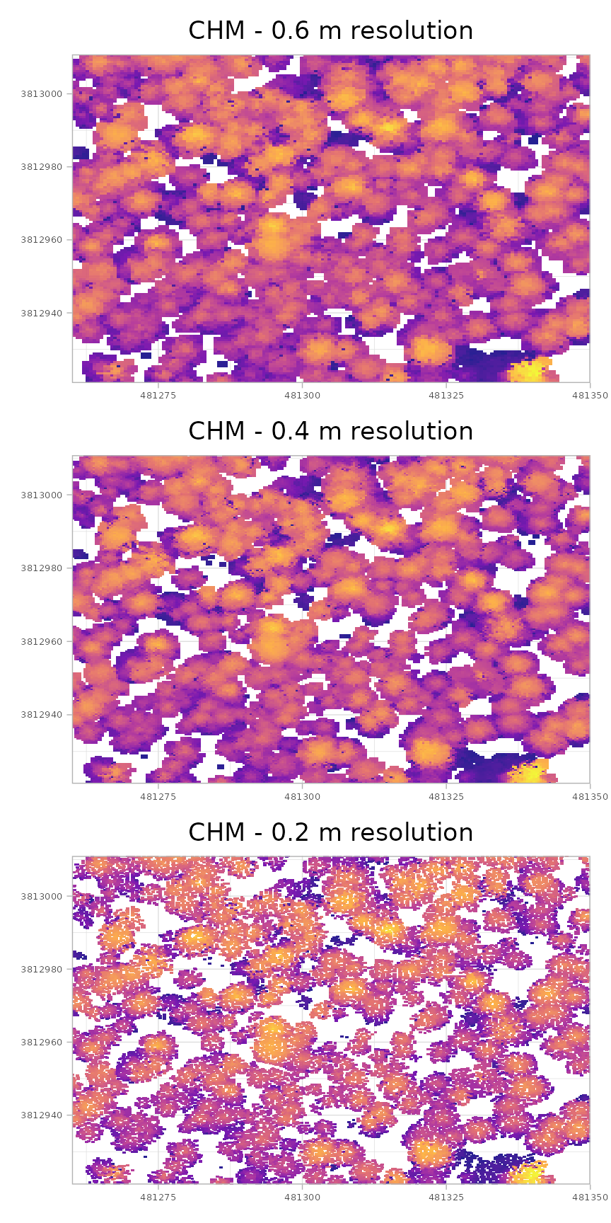

As you transition from the coarser resolution CHM (0.6 m) to the finest resolution CHM (0.2 m), several changes are apparent. The first difference relates to canopy coverage: coarser resolution data covers more area above the minimum height threshold. This occurs because the larger cell size forces the raster to search a broader area for the highest non-ground point, effectively smoothing the point cloud data and reducing fine detail and small gaps. Conversely, finer resolution data makes crown gaps more apparent, but this increased detail comes with the risk of introducing “holes” within what should be continuous individual tree crowns (an effect that can be mitigated with post-processing smoothing). Furthermore, the finer resolution CHM better resolves small trees, making them more apparent in the product. While using a finer resolution CHM has been shown to improve both tree detection and tree crown area accuracy, a trade-off must be considered as the 0.2 m resolution product generates 9 times the amount of data to store and process compared to the 0.6 m resolution product.

A simple rule of thumb for determining how fine a CHM to generate is to ensure there is at least one point per cell in the target CHM. To find the minimum CHM resolution that could be created for a given point density (i.e. points m^-2) while maintaining this threshold, use the formula $\sqrt{1/\text{point_density}}$. For example, a point density of 17 points m^-2 could generate a minimum CHM resolution of approximately 0.24 m ($\sqrt{1/17} \approx 0.24$) while ensuring at least one point per cell on average. Alternatively, to find the minimum point density needed to support a desired CHM resolution, use the formula $1/(\text{desired_res}^2)$. For instance, creating a 0.3 m CHM raster requires point cloud data with at least 11.11 points m^-2 ($1/(0.3^2) \approx 11.11$).

Unfiltered Maximum CHM

We can also generate an unfiltered maximum CHM which is a raster layer generated from a height-normalized point cloud using maximum Z-value interpolation, where the “unfiltered” characteristic means no minimum or maximum height threshold is applied to mask out values. This process ensures the resulting CHM captures the maximum vertical extent of all above-ground features, from the tallest canopy down to the smallest ground debris. The unfilterd CHM represents the height of the highest object found directly above the ground in every cell. This type of raster data is distinct from a Digital Surface Model (DSM), which represents the total elevation including the ground itself, and a Digital Terrain Model (DTM), which only represents the bare earth elevation.

The primary benefit of generating an unfiltered CHM is the analysis flexibility it enables, as it includes all non-ground data. Because no information is masked out during generation, the data can be “sliced” in post-processing to look at specific height ranges of interest without needing to regenerate the CHM. For example, in forestry management, a single unfiltered CHM can be used to filter for trees only (e.g. set a threshold above 2 m) or filter for understory vegetation and other objects (e.g. isolate features between 0.3 m and 2.2 m). This allows for analysis of different forest strata using a single initial dataset.

To further enhance analysis flexibility and avoid repeating the computationally expensive point cloud processing, we strongly advise generating the CHM at the finest resolution that might be required for analysis. It is far more efficient to later aggregate a fine resolution raster (for instance, taking a 0.5 m resolution raster and aggregating it to a more coarse 2.0 m resolution) than it is to re-run the entire pipeline.

Here we’ll demonstrate how to generate an unfiltered maximum CHM, “slice” the CHM to look at a specific height range, and aggregate it to a more coarse resolution.

The key settings to ensure the resulting CHM is unfiltered are the min_height = 0 and max_height = Inf arguments

# unfiltered chm
cloud2raster_ans_chm_unfiltered <- cloud2trees::cloud2raster(
  input_las_dir = las_dir
  , output_dir = out_dir
  , chm_res_m = 0.2
  , min_height = 0
  , max_height = Inf
)

let’s compare this unfiltered CHM to the first 0.2 m resolution raster we created which was height filtered based on the default min_height = 2 and max_height = 70 arguments

plt_chm_unfiltered <- 
 cloud2raster_ans_chm_unfiltered$chm_rast %>%
  terra::as.data.frame(xy=T) %>%
  dplyr::rename(f=3) %>%
  ggplot2::ggplot() +
  ggplot2::geom_tile(
    mapping = ggplot2::aes(x=x, y=y, fill=f)
    , alpha = 0.9
  ) +
  ggplot2::scale_fill_viridis_c(option = "plasma") +
  ggplot2::scale_x_continuous(expand = c(0, 0)) +
  ggplot2::scale_y_continuous(expand = c(0, 0)) +
  ggplot2::labs(fill = "CHM (m)", title = "CHM - Unfiltered Height") +
  ggplot2::theme_light() +
  ggplot2::theme(
    legend.position = "none"
    , axis.text = ggplot2::element_text(size = 5)
    , axis.title = ggplot2::element_blank()
    , plot.title = ggplot2::element_text(hjust = 0.5)
  )
# update title on the filtered
plt_chm_0.2m <- plt_chm_0.2m + ggplot2::labs(title = "CHM - Filtered Height")

combine with patchwork::wrap_plots()

# patchwork
patchwork::wrap_plots(plt_chm_unfiltered, plt_chm_0.2m, ncol = 2)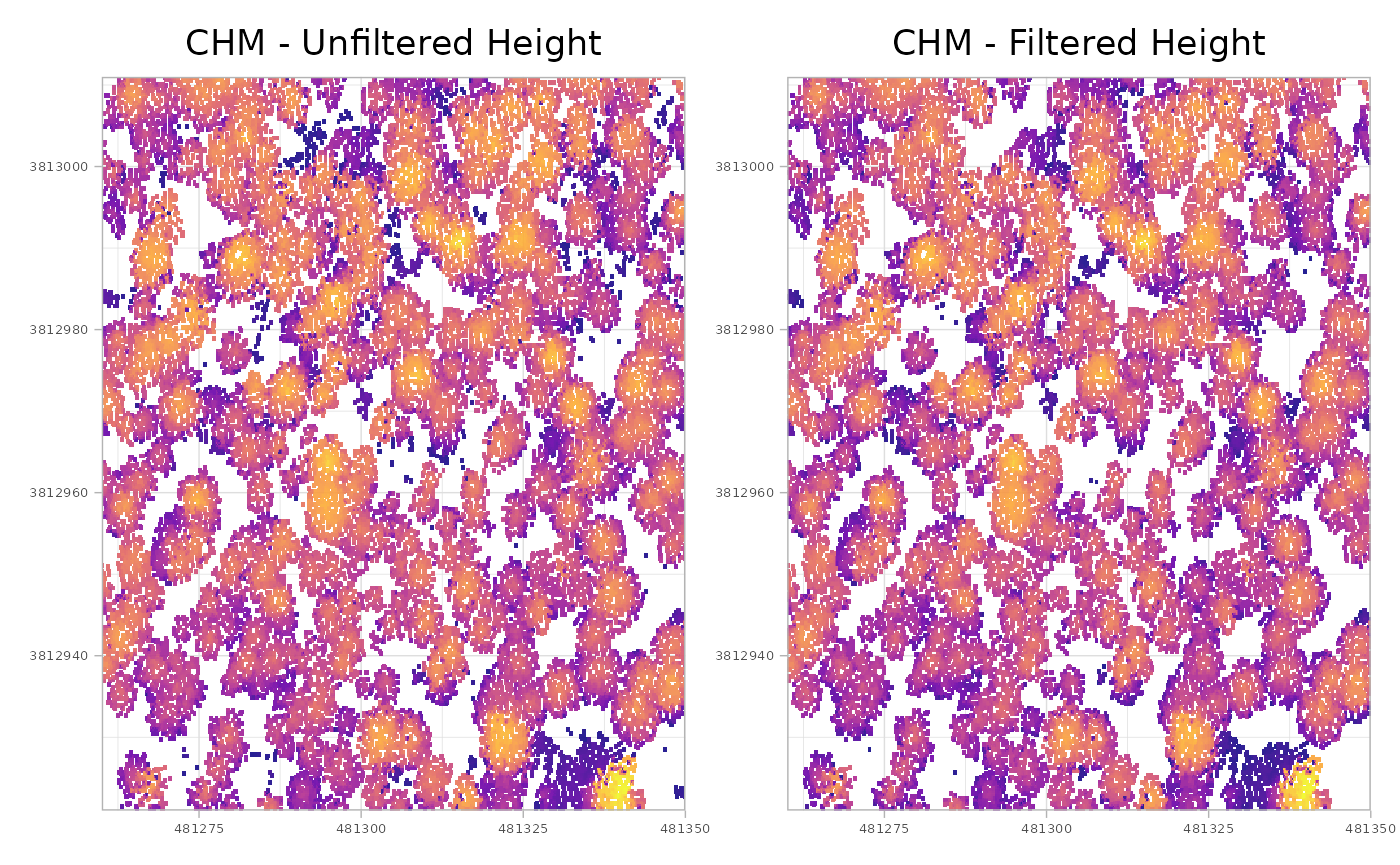

that might be difficult to see, so let’s create a difference raster for easier comparison

# differnece raster
terra::ifel(
    is.na(cloud2raster_ans_chm_0.2m$chm_rast)
    , cloud2raster_ans_chm_unfiltered$chm_rast
    , cloud2raster_ans_chm_unfiltered$chm_rast - cloud2raster_ans_chm_0.2m$chm_rast
  ) %>% 
  # dichotomous non-zero difference
  `!=`(0) %>% 
  # plot it
  terra::plot(col = c("gray","firebrick"), main = "differences shown in red")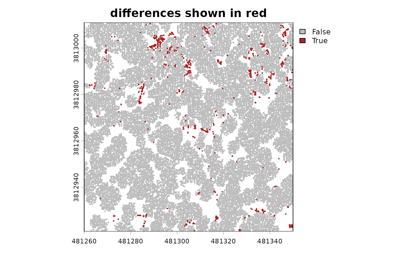

now, let’s “slice” the unfiltered CHM to look for possible lower vegetation between 0.3 m and 2.2 m that is not directly underneath taller objects (which would occlude these objects in the CHM)

terra::ifel(
    cloud2raster_ans_chm_unfiltered$chm_rast >= 0.3 & 
    cloud2raster_ans_chm_unfiltered$chm_rast <= 2.2
    , cloud2raster_ans_chm_unfiltered$chm_rast 
    , NA
  ) %>% 
  terra::plot(col = rev(grDevices::hcl.colors(55, "Peach")))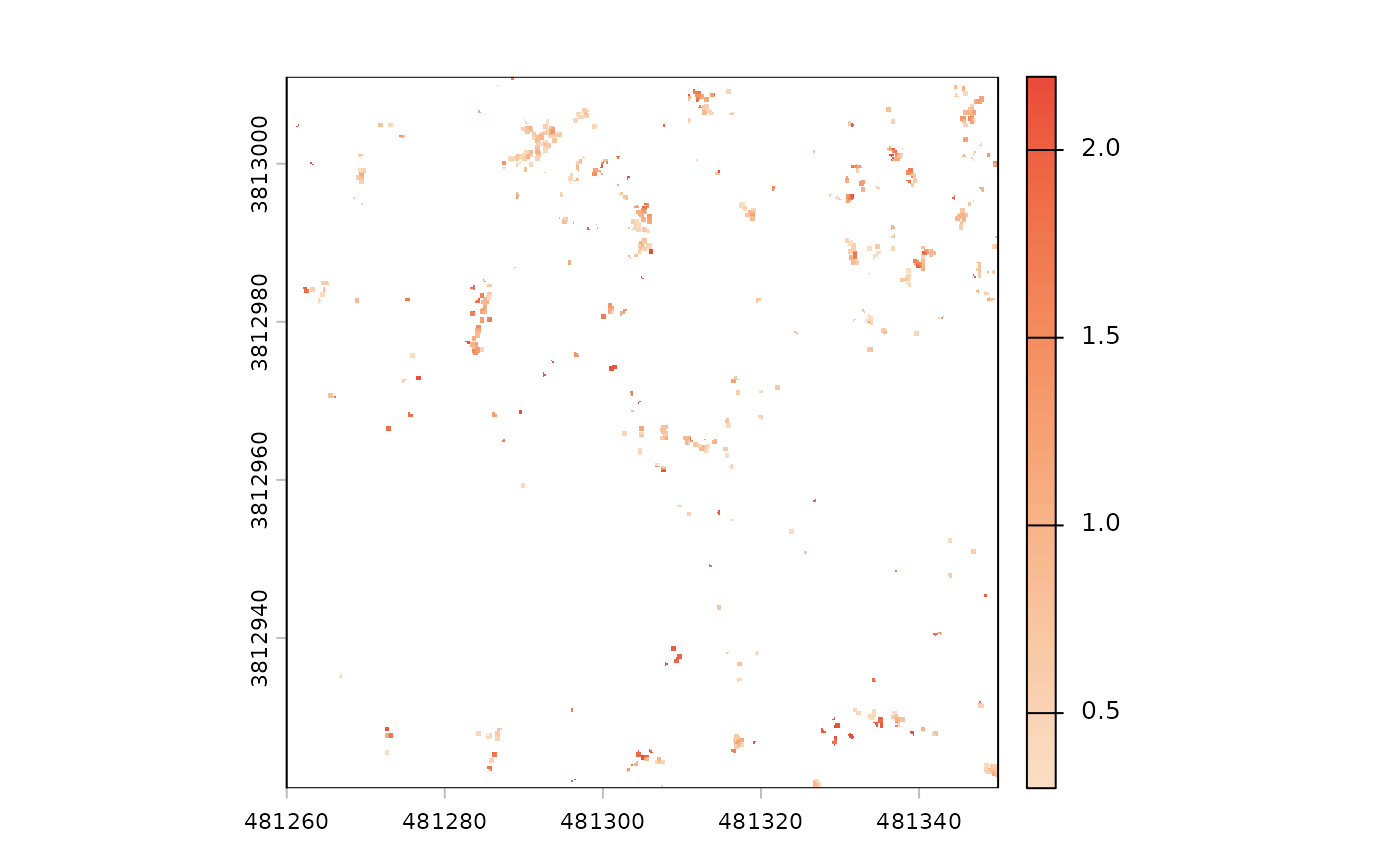

finally, we can make the fine resolution (0.2 m) CHM raster more coarse (0.4 m) using terra::aggregate() and we’ll display the resultant resolution in the X and Y horizontal

terra::aggregate(
    cloud2raster_ans_chm_unfiltered$chm_rast
    , fact = 2
    , fun = "max"
  ) %>% 
  terra::res() %>% 
  paste(collapse = "x")
#> [1] "0.4x0.4"