Section 4 Point Cloud Generation and Processing

4.1 SfM Image Processing Data

We tracked the photogrammetry (SfM) data generation processing times across the software platforms. Bring in this data and combine it as it has slightly different structure. The software packages were all run on different machines which means we need to figure out a way to standardize the image processing time to compare across software.

Load the file with ODM and Pix4D image processing data

odm_pix_temp = 
  readr::read_csv("../data/sfm_processing_time.csv") %>% 
  dplyr::rename_with(~ .x %>% 
    stringr::str_squish() %>% 
    str_remove_all("[[:punct:]]") %>% 
    stringr::str_replace_all("\\s","_") %>% 
    tolower()
  ) %>% 
  # map the processing parameters to the columns in our current data str
  dplyr::mutate(
    software = software %>% 
      stringr::str_remove_all("\\s") %>% 
      toupper()
    , processing_attribute1 = dplyr::case_when(
        software == "PIX4D" ~ keypoint_image_scale
        , T ~ depth_map_quality
      )
    , processing_attribute2 = dplyr::case_when(
        software == "PIX4D" ~ depth_map_quality
        , T ~ filtering_mode
      )
    , processing_attribute3 = dplyr::case_when(
        software == "PIX4D" ~ filtering_mode
        , T ~ as.character(NA)
      )
  ) %>% 
  # clean the data
  dplyr::mutate(
    dplyr::across(
      tidyselect::starts_with("processing_attribute")
      , ~ .x %>% 
        stringr::str_remove_all("\\s") %>% 
        toupper()
    )
    , site = site %>% 
      stringr::str_squish() %>% 
      stringr::str_replace_all("\\s","_") %>% 
      stringr::str_replace_all("[^[:alnum:]]","_") %>% 
      toupper()
  ) %>%
  # filter pix4d for only original
  dplyr::filter(
    dplyr::case_when(
      tolower(software) == "pix4d" & tolower(processing_attribute1) == "original" ~ T
      , tolower(software) != "pix4d" ~ T
      , T ~ F
    ) == T
  ) %>% 
  dplyr::mutate(
    # temporary
    qqq = dplyr::case_when(
        tolower(software) == "pix4d" ~ processing_attribute2
        , T ~ processing_attribute1
      )
    , fff = dplyr::case_when(
        tolower(software) == "pix4d" ~ processing_attribute3
        , T ~ processing_attribute2
      )
  ) %>% 
  dplyr::rename(
    study_site = site
    , total_sfm_time_min = total_generation_time_min
    , number_of_points_sfm = pc_total_number
  ) %>% 
  # select columns we need for joining
  dplyr::select(
    software
    , study_site
    , total_sfm_time_min
    , number_of_points_sfm
    , qqq
    , fff
  ) 

clean up the metashape image processing data and combine with odm and pix4d

# clean up the metashape image processing data and combine with odm and pix4d
ms_temp = readr::read_csv("../data/metashape_processing_data.csv")
sfm_comb_temp = ms_temp %>% 
  dplyr::mutate(
    software = toupper("metashape")
    , total_sfm_time_min = 
      total_dense_point_cloud_processing_time_mins +
      total_sparse_point_cloud_processing_time_mins
    , number_of_points_sfm = dense_point_cloud_points
    , qqq = depth_maps_generation_quality
    , fff = depth_maps_generation_filtering_mode
  ) %>% 
  dplyr::select(names(odm_pix_temp)) %>% 
  dplyr::bind_rows(odm_pix_temp) %>% 
  # map quality and filtering to match above
  dplyr::mutate(
    # mapping 
    depth_maps_generation_quality = dplyr::case_when(
        tolower(qqq) %in% c("ultrahigh", "ultra", "original", "origianl") ~ "ultra high"
        , tolower(qqq) %in% c("half") ~ "high"
        , tolower(qqq) %in% c("quarter") ~ "medium"
        , tolower(qqq) %in% c("eighth","eightht") ~ "low"
        , T ~ tolower(qqq)
      ) %>% 
      factor(
        ordered = TRUE
        , levels = c(
          "lowest"
          , "low"
          , "medium"
          , "high"
          , "ultra high"
        )
      ) %>% forcats::fct_rev()
    , depth_maps_generation_filtering_mode = dplyr::case_when(
        tolower(fff) %in% c("high") & 
          tolower(software) %in% c("opendronemap") ~ "disabled"
        , tolower(fff) %in% c("high")
          & tolower(software) %in% c("pix4d") ~ "disabled"
        , tolower(fff) %in% c("medium")
          & tolower(software) %in% c("opendronemap") ~ "mild"
        , tolower(fff) %in% c("optimal")
          & tolower(software) %in% c("pix4d") ~ "mild"
        , tolower(fff) %in% c("low")
          & tolower(software) %in% c("opendronemap") ~ "moderate"
        , tolower(fff) %in% c("low")
          & tolower(software) %in% c("pix4d") ~ "moderate"
        , tolower(fff) %in% c("lowest")
          & tolower(software) %in% c("opendronemap") ~ "aggressive"
        , T ~ tolower(fff)
      ) %>% 
      factor(
        ordered = TRUE
        , levels = c(
          "disabled"
          , "mild"
          , "moderate"
          , "aggressive"
        )
      ) %>% forcats::fct_rev()
  ) %>% 
  dplyr::select(-c(qqq,fff)) %>% 
  # keep only one thing record
  dplyr::group_by(
    software, study_site, depth_maps_generation_quality, depth_maps_generation_filtering_mode
  ) %>% 
  dplyr::filter(dplyr::row_number()==1) %>% 
  dplyr::ungroup()

What?

sfm_comb_temp %>% dplyr::glimpse()

## Rows: 342
## Columns: 6
## $ software                             <chr> "METASHAPE", "METASHAPE", "METASH…
## $ study_site                           <chr> "KAIBAB_HIGH", "KAIBAB_HIGH", "KA…
## $ total_sfm_time_min                   <dbl> 209.600000, 232.600000, 206.60000…
## $ number_of_points_sfm                 <dbl> 225918417, 305690646, 295828394, …
## $ depth_maps_generation_quality        <ord> ultra high, ultra high, ultra hig…
## $ depth_maps_generation_filtering_mode <ord> aggressive, moderate, mild, disab…

4.2 R Point Cloud Processing Data

The point cloud files (.las|.laz files) exported by the SfM software platforms (Metashape, Pix4D, and OpenDroneMap) were processed in R using the process outlined in the manuscript and implemented via the cloud2trees() function from the cloud2trees package by Woolsey and Tinkham (2024). This process was completed for all 260 data sets to be analyzed based on the different combinations of SfM parameter settings tested (100 from both Metashape and OpenDroneMap and 60 from Pix4D).

We saved the processed data in the directory which we call ptcld_processing_dir in the code below organized as ptcld_processing_dir/software/study_site/parameter1_parameter2.csv where parameter1 and parameter2 are the SfM algorithm parameter settings (e.g. dense cloud generation quality and filtering mode). The processing tracking data file is used to compare summary statistics on point cloud processing times and densities.

For comparison across software, the SfM point cloud generation processing parameters are mapped to the Metashape parameters based on the Pix4D documentation, the OpenDroneMap documentation, and the Agisoft Metashape discussion board

### get tracking data
 # read list of all processed tracking files
  tracking_list_df =
    dplyr::tibble(
      file_full_path = list.files(
          ptcld_processing_dir
          , pattern = ".*_processed_tracking_data\\.csv$"
          , full.names = T, recursive = T
        ) %>% 
        normalizePath()
    ) %>% 
    # get the software used
    dplyr::mutate(
      file_full_path %>% 
        toupper() %>%
        stringr::str_extract_all(pattern = paste(toupper(software_list),collapse = "|"), simplify = T) %>% 
        dplyr::as_tibble() %>% 
        tidyr::unite(col = "software", sep = " ", na.rm = T)
    ) %>% 
    # filter processed tracking files
    dplyr::mutate(
      software = software %>% stringr::word(-1)
      , study_site = file_full_path %>%
        toupper() %>%
        stringr::str_extract(pattern = paste(toupper(study_site_list),collapse = "|"))
      , file_name = file_full_path %>%
        basename() %>%
        stringr::word(1, sep = fixed(".")) %>%
        toupper() %>%
        stringr::str_remove_all("_PROCESSED_TRACKING_DATA")
    ) %>% 
    dplyr::filter(
      !is.na(study_site)
      & study_site %in% toupper(study_site_list)
      & !is.na(software)
      & software %in% toupper(software_list)
    ) %>% 
    # keep only unique files for processing
    dplyr::group_by(software, study_site, file_name) %>%
    dplyr::filter(dplyr::row_number()==1) %>%
    dplyr::ungroup() %>%
    dplyr::rename(tracking_file_full_path = file_full_path)

What? Here, there are 500 files because we also created data using image alignment other than “Original” in Pix4D but keep only the “Original” files for final analysis.

tracking_list_df %>% dplyr::glimpse()

## Rows: 500
## Columns: 4
## $ tracking_file_full_path <chr> "E:\\SfM_Software_Comparison\\Metashape\\point…
## $ software                <chr> "METASHAPE", "METASHAPE", "METASHAPE", "METASH…
## $ study_site              <chr> "KAIBAB_HIGH", "KAIBAB_HIGH", "KAIBAB_HIGH", "…
## $ file_name               <chr> "HIGH_AGGRESSIVE", "HIGH_DISABLED", "HIGH_MILD…

read each tracking data file, bind rows

# read each tracking data file, bind rows
  ptcld_processing_data = 1:nrow(tracking_list_df) %>%
    purrr::map(function(row_n){
      tracking_list_df %>%
        dplyr::filter(dplyr::row_number() == row_n) %>%
        dplyr::bind_cols(
          read.csv(tracking_list_df$tracking_file_full_path[row_n]) 
        )
    }) %>%
    dplyr::bind_rows()

What?

ptcld_processing_data %>% dplyr::glimpse()

## Rows: 500
## Columns: 26
## $ tracking_file_full_path            <chr> "E:\\SfM_Software_Comparison\\Metas…
## $ software                           <chr> "METASHAPE", "METASHAPE", "METASHAP…
## $ study_site                         <chr> "KAIBAB_HIGH", "KAIBAB_HIGH", "KAIB…
## $ file_name                          <chr> "HIGH_AGGRESSIVE", "HIGH_DISABLED",…
## $ number_of_points                   <int> 52974294, 72549206, 69858217, 69825…
## $ las_area_m2                        <dbl> 86661.27, 87175.42, 86404.78, 86413…
## $ timer_tile_time_mins               <dbl> 0.63600698, 2.49318542, 0.84133803,…
## $ timer_class_dtm_norm_chm_time_mins <dbl> 3.6559556, 5.3289152, 5.1638296, 5.…
## $ timer_treels_time_mins             <dbl> 8.9065272, 19.2119663, 12.3391793, …
## $ timer_itd_time_mins                <dbl> 0.02202115, 0.02449968, 0.03798440,…
## $ timer_competition_time_mins        <dbl> 0.10590740, 0.17865245, 0.12124869,…
## $ timer_estdbh_time_mins             <dbl> 0.02290262, 0.02382533, 0.02199170,…
## $ timer_silv_time_mins               <dbl> 0.012565533, 0.015940932, 0.0150339…
## $ timer_total_time_mins              <dbl> 13.361886, 27.276985, 18.540606, 17…
## $ sttng_input_las_dir                <chr> "D:/Metashape_Testing_2024", "D:/Me…
## $ sttng_use_parallel_processing      <lgl> FALSE, FALSE, FALSE, FALSE, FALSE, …
## $ sttng_desired_chm_res              <dbl> 0.25, 0.25, 0.25, 0.25, 0.25, 0.25,…
## $ sttng_max_height_threshold_m       <int> 60, 60, 60, 60, 60, 60, 60, 60, 60,…
## $ sttng_minimum_tree_height_m        <int> 2, 2, 2, 2, 2, 2, 2, 2, 2, 2, 2, 2,…
## $ sttng_dbh_max_size_m               <int> 2, 2, 2, 2, 2, 2, 2, 2, 2, 2, 2, 2,…
## $ sttng_local_dbh_model              <chr> "rf", "rf", "rf", "rf", "rf", "rf",…
## $ sttng_user_supplied_epsg           <lgl> NA, NA, NA, NA, NA, NA, NA, NA, NA,…
## $ sttng_accuracy_level               <int> 2, 2, 2, 2, 2, 2, 2, 2, 2, 2, 2, 2,…
## $ sttng_pts_m2_for_triangulation     <int> 20, 20, 20, 20, 20, 20, 20, 20, 20,…
## $ sttng_normalization_with           <chr> "triangulation", "triangulation", "…
## $ sttng_competition_buffer_m         <int> 5, 5, 5, 5, 5, 5, 5, 5, 5, 5, 5, 5,…

split file name to get processing attributes

# split file name to get processing attributes
    ptcld_processing_data =
      ptcld_processing_data %>%
      tidyr::separate_wider_delim(
        cols = file_name
        , delim = "_"
        , names = paste0(
            "processing_attribute"
            , 1:(max(stringr::str_count(ptcld_processing_data$file_name, "_"))+1)
          )
        , too_few = "align_start"
        , cols_remove = F
      ) %>%
      # not sure how to map processing attributes for pix4d and opendronemap ??????????????
      dplyr::mutate(
        # temporary
        qqq = dplyr::case_when(
            tolower(software) == "pix4d" ~ processing_attribute2
            , T ~ processing_attribute1
          )
        , fff = dplyr::case_when(
            tolower(software) == "pix4d" ~ processing_attribute3
            , T ~ processing_attribute2
          )
        # mapping 
        , depth_maps_generation_quality = dplyr::case_when(
            tolower(qqq) %in% c("ultrahigh", "ultra", "original", "origianl") ~ "ultra high"
            , tolower(qqq) %in% c("half") ~ "high"
            , tolower(qqq) %in% c("quarter") ~ "medium"
            , tolower(qqq) %in% c("eighth","eightht") ~ "low"
            , T ~ tolower(qqq)
          ) %>% 
          factor(
            ordered = TRUE
            , levels = c(
              "lowest"
              , "low"
              , "medium"
              , "high"
              , "ultra high"
            )
          ) %>% forcats::fct_rev()
        , depth_maps_generation_filtering_mode = dplyr::case_when(
            tolower(fff) %in% c("high") & 
              tolower(software) %in% c("opendronemap") ~ "disabled"
            , tolower(fff) %in% c("high")
              & tolower(software) %in% c("pix4d") ~ "disabled"
            , tolower(fff) %in% c("medium")
              & tolower(software) %in% c("opendronemap") ~ "mild"
            , tolower(fff) %in% c("optimal")
              & tolower(software) %in% c("pix4d") ~ "mild"
            , tolower(fff) %in% c("low")
              & tolower(software) %in% c("opendronemap") ~ "moderate"
            , tolower(fff) %in% c("low")
              & tolower(software) %in% c("pix4d") ~ "moderate"
            , tolower(fff) %in% c("lowest")
              & tolower(software) %in% c("opendronemap") ~ "aggressive"
            , T ~ tolower(fff)
          ) %>% 
          factor(
            ordered = TRUE
            , levels = c(
              "disabled"
              , "mild"
              , "moderate"
              , "aggressive"
            )
          ) %>% forcats::fct_rev()
      )

what have we done?

ptcld_processing_data %>% dplyr::glimpse()

## Rows: 500
## Columns: 33
## $ tracking_file_full_path              <chr> "E:\\SfM_Software_Comparison\\Met…
## $ software                             <chr> "METASHAPE", "METASHAPE", "METASH…
## $ study_site                           <chr> "KAIBAB_HIGH", "KAIBAB_HIGH", "KA…
## $ processing_attribute1                <chr> "HIGH", "HIGH", "HIGH", "HIGH", "…
## $ processing_attribute2                <chr> "AGGRESSIVE", "DISABLED", "MILD",…
## $ processing_attribute3                <chr> NA, NA, NA, NA, NA, NA, NA, NA, N…
## $ file_name                            <chr> "HIGH_AGGRESSIVE", "HIGH_DISABLED…
## $ number_of_points                     <int> 52974294, 72549206, 69858217, 698…
## $ las_area_m2                          <dbl> 86661.27, 87175.42, 86404.78, 864…
## $ timer_tile_time_mins                 <dbl> 0.63600698, 2.49318542, 0.8413380…
## $ timer_class_dtm_norm_chm_time_mins   <dbl> 3.6559556, 5.3289152, 5.1638296, …
## $ timer_treels_time_mins               <dbl> 8.9065272, 19.2119663, 12.3391793…
## $ timer_itd_time_mins                  <dbl> 0.02202115, 0.02449968, 0.0379844…
## $ timer_competition_time_mins          <dbl> 0.10590740, 0.17865245, 0.1212486…
## $ timer_estdbh_time_mins               <dbl> 0.02290262, 0.02382533, 0.0219917…
## $ timer_silv_time_mins                 <dbl> 0.012565533, 0.015940932, 0.01503…
## $ timer_total_time_mins                <dbl> 13.361886, 27.276985, 18.540606, …
## $ sttng_input_las_dir                  <chr> "D:/Metashape_Testing_2024", "D:/…
## $ sttng_use_parallel_processing        <lgl> FALSE, FALSE, FALSE, FALSE, FALSE…
## $ sttng_desired_chm_res                <dbl> 0.25, 0.25, 0.25, 0.25, 0.25, 0.2…
## $ sttng_max_height_threshold_m         <int> 60, 60, 60, 60, 60, 60, 60, 60, 6…
## $ sttng_minimum_tree_height_m          <int> 2, 2, 2, 2, 2, 2, 2, 2, 2, 2, 2, …
## $ sttng_dbh_max_size_m                 <int> 2, 2, 2, 2, 2, 2, 2, 2, 2, 2, 2, …
## $ sttng_local_dbh_model                <chr> "rf", "rf", "rf", "rf", "rf", "rf…
## $ sttng_user_supplied_epsg             <lgl> NA, NA, NA, NA, NA, NA, NA, NA, N…
## $ sttng_accuracy_level                 <int> 2, 2, 2, 2, 2, 2, 2, 2, 2, 2, 2, …
## $ sttng_pts_m2_for_triangulation       <int> 20, 20, 20, 20, 20, 20, 20, 20, 2…
## $ sttng_normalization_with             <chr> "triangulation", "triangulation",…
## $ sttng_competition_buffer_m           <int> 5, 5, 5, 5, 5, 5, 5, 5, 5, 5, 5, …
## $ qqq                                  <chr> "HIGH", "HIGH", "HIGH", "HIGH", "…
## $ fff                                  <chr> "AGGRESSIVE", "DISABLED", "MILD",…
## $ depth_maps_generation_quality        <ord> high, high, high, high, low, low,…
## $ depth_maps_generation_filtering_mode <ord> aggressive, disabled, mild, moder…

what is this mapping?

# quality
ptcld_processing_data %>% 
  dplyr::count(depth_maps_generation_quality, qqq, software) %>% 
  ggplot(aes(x = tolower(software), y = depth_maps_generation_quality, label = tolower(qqq))) +
    geom_tile(fill = NA, color = "black") +
    ggrepel::geom_text_repel(color = "gray33") +
    labs(y = "Mapped: Depth Map Quality", x = "") +
    scale_x_discrete(position = "top") +
    coord_cartesian(expand = F) +
    theme_light() +
    theme(
      panel.grid = element_blank()
      , axis.text = element_text(size = 11, face = "bold", color = "black")
      , panel.border = element_rect(color = "black")
    )

ggplot2::ggsave("../data/mapped_quality.jpg", height = 8, width = 6)

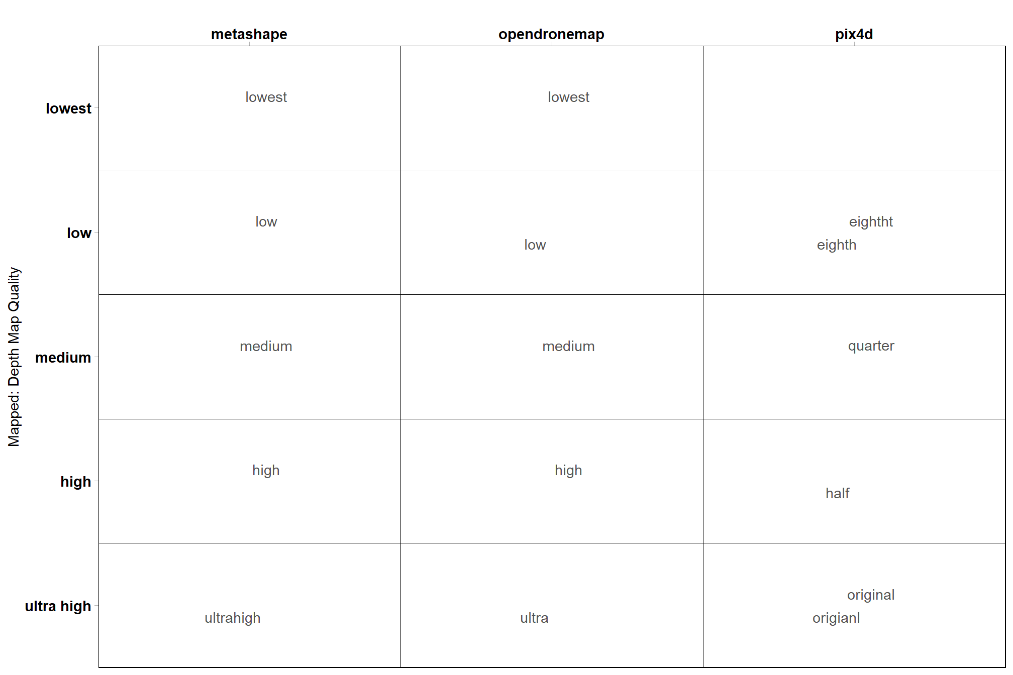
notice the spelling errors in the file names…manual file naming can be a dangerous game to play.

# filtering
ptcld_processing_data %>% 
  dplyr::count(depth_maps_generation_filtering_mode, fff, software) %>% 
  ggplot(aes(x = tolower(software), y = depth_maps_generation_filtering_mode, label = tolower(fff))) +
    geom_tile(fill = NA, color = "black") +
    ggrepel::geom_text_repel(color = "gray33") +
    labs(y = "Mapped: Filtering Mode", x = "") +
    scale_x_discrete(position = "top") +
    coord_cartesian(expand = F) +
    theme_light() +
    theme(
      panel.grid = element_blank()
      , axis.text = element_text(size = 11, face = "bold", color = "black")
      , panel.border = element_rect(color = "black")
    )

ggplot2::ggsave("../data/mapped_filtering_mode.jpg", height = 8, width = 6)

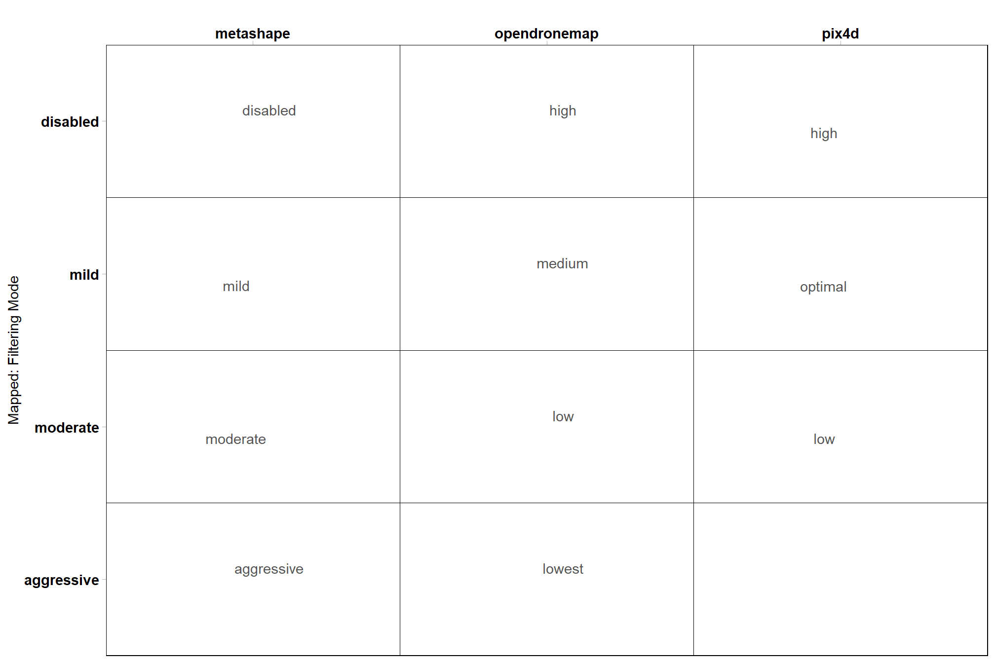
let’s filter out those extra Pix4D data sets

ptcld_processing_data = ptcld_processing_data %>% 
  dplyr::select(-c(qqq,fff)) %>% 
  dplyr::filter(
    dplyr::case_when(
      tolower(software) == "pix4d" & tolower(processing_attribute1) == "original" ~ T
      , tolower(software) != "pix4d" ~ T
      , T ~ F
    ) == T
  )

4.3 Summary of Data Generation and Processing

join the SfM data generation to the processing data which we’ll use to build our full analysis data set and create the normalized processing time using Min-Max normalization.

ptcld_processing_data = ptcld_processing_data %>% 
  dplyr::left_join(
    sfm_comb_temp
    , by = dplyr::join_by(
      software, study_site, depth_maps_generation_quality, depth_maps_generation_filtering_mode
    )
  ) %>% 
  # create the standardized time by software since the processing machine varied by software
  dplyr::group_by(software) %>% 
  dplyr::mutate(
    total_sfm_time_norm = (total_sfm_time_min-min(total_sfm_time_min, na.rm = T)) /
      (max(total_sfm_time_min, na.rm = T)-min(total_sfm_time_min, na.rm = T))
  ) %>% 
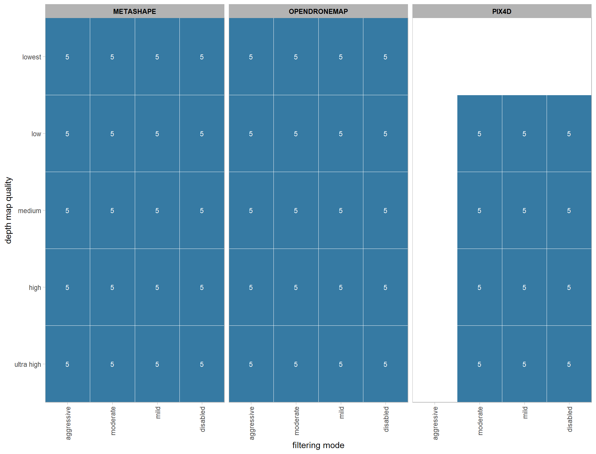
  dplyr::ungroup()

4.3.1 Number of files summary

ptcld_processing_data %>% 
  dplyr::count(software, depth_maps_generation_quality, depth_maps_generation_filtering_mode) %>% 
  ggplot(mapping = aes(
    y = depth_maps_generation_quality
    , x = depth_maps_generation_filtering_mode
    , fill = n
    , label = n
  )) +
  geom_tile(color = "white") +
  geom_text(color = "white", size = 3) +
  facet_grid(cols = vars(software)) + 
  scale_x_discrete(expand = c(0, 0)) +
  scale_y_discrete(expand = c(0, 0)) +
  scale_fill_viridis_c(option = "mako", direction=-1, begin = 0.2, end = 0.8) +
  labs(
    x = "filtering mode"
    , y = "depth map quality"
    , fill = "number of sites"
  ) +
  theme_light() + 
  theme(
    legend.position = "none"
    , axis.text.x = element_text(angle = 90, vjust = 0.5, hjust = 1)
    , panel.background = element_blank()
    , panel.grid = element_blank()
    , plot.subtitle = element_text(hjust = 0.5)
    , strip.text = element_text(color = "black", face = "bold")
  )

4.3.2 R Processing Time Summary

Total processing time by depth map generation quality and depth map filtering mode

ptcld_processing_data %>% 
  ggplot(
    mapping = aes(
      x = depth_maps_generation_quality
      , y = timer_total_time_mins
      , color = depth_maps_generation_filtering_mode
      , fill = depth_maps_generation_filtering_mode
    )
  ) +
  geom_boxplot(alpha = 0.6) +
  scale_color_viridis_d(option = "plasma") +
  scale_fill_viridis_d(option = "plasma") +
  scale_y_log10(
    labels = scales::comma_format(suffix = " mins", accuracy = 1)
    , breaks = scales::breaks_log(n = 9)
  ) +
  labs(
    color = "Filtering Mode"
    , fill = "Filtering Mode"
    , y = "Point Cloud Total Processing Time"
    , x = "Quality"
    , title = bquote(
        bold("R") ~
        "point cloud total processing time by depth map generation quality and filtering mode"
    )
    , caption = "*Note the log scale on the y-axis"
  ) +
  theme_light() +
  theme(
    legend.position = "top"
    , legend.direction  = "horizontal"
  ) +
  guides(
    color = guide_legend(override.aes = list(shape = 15, size = 6, alpha = 0.9))
  )

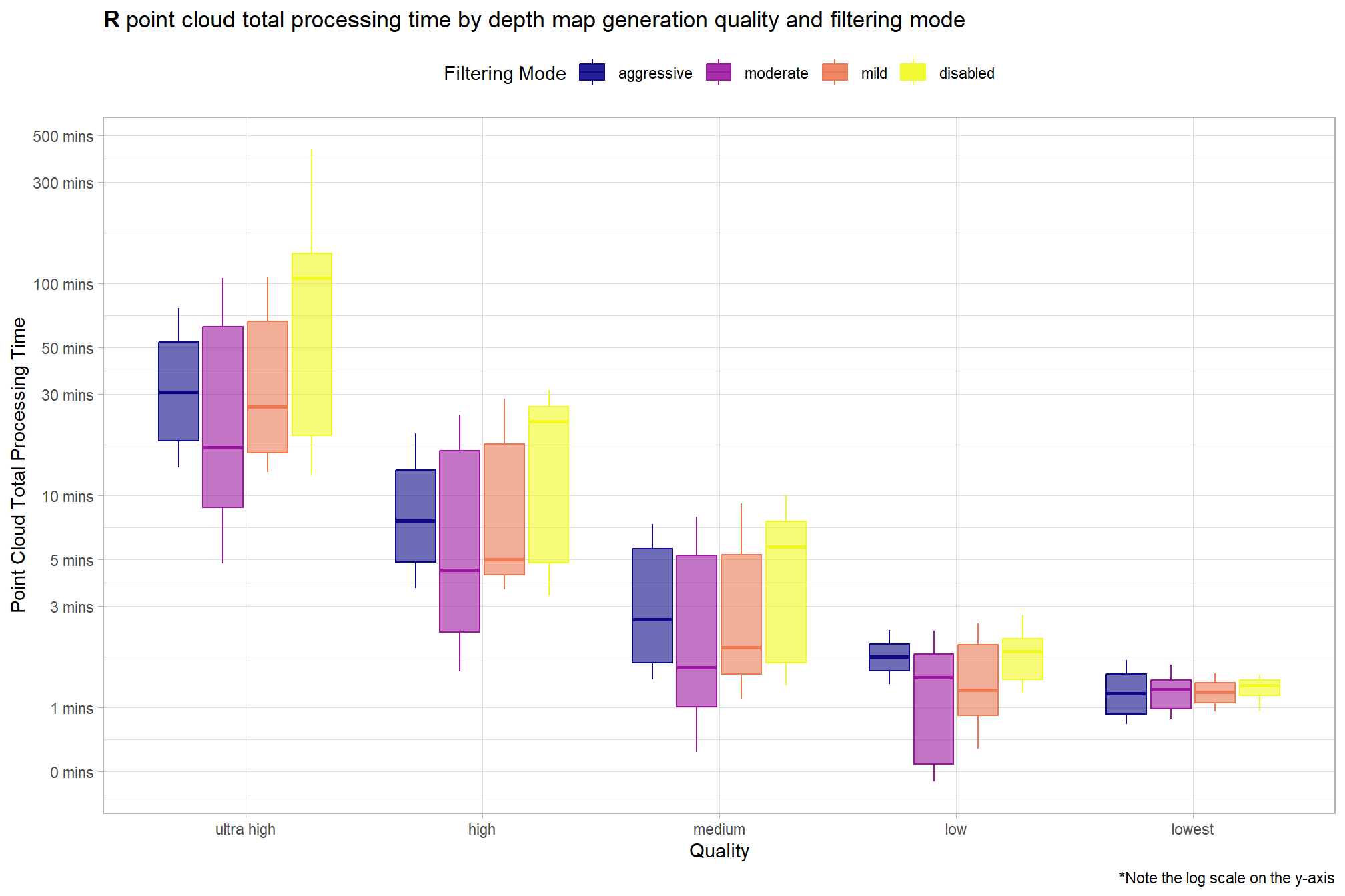
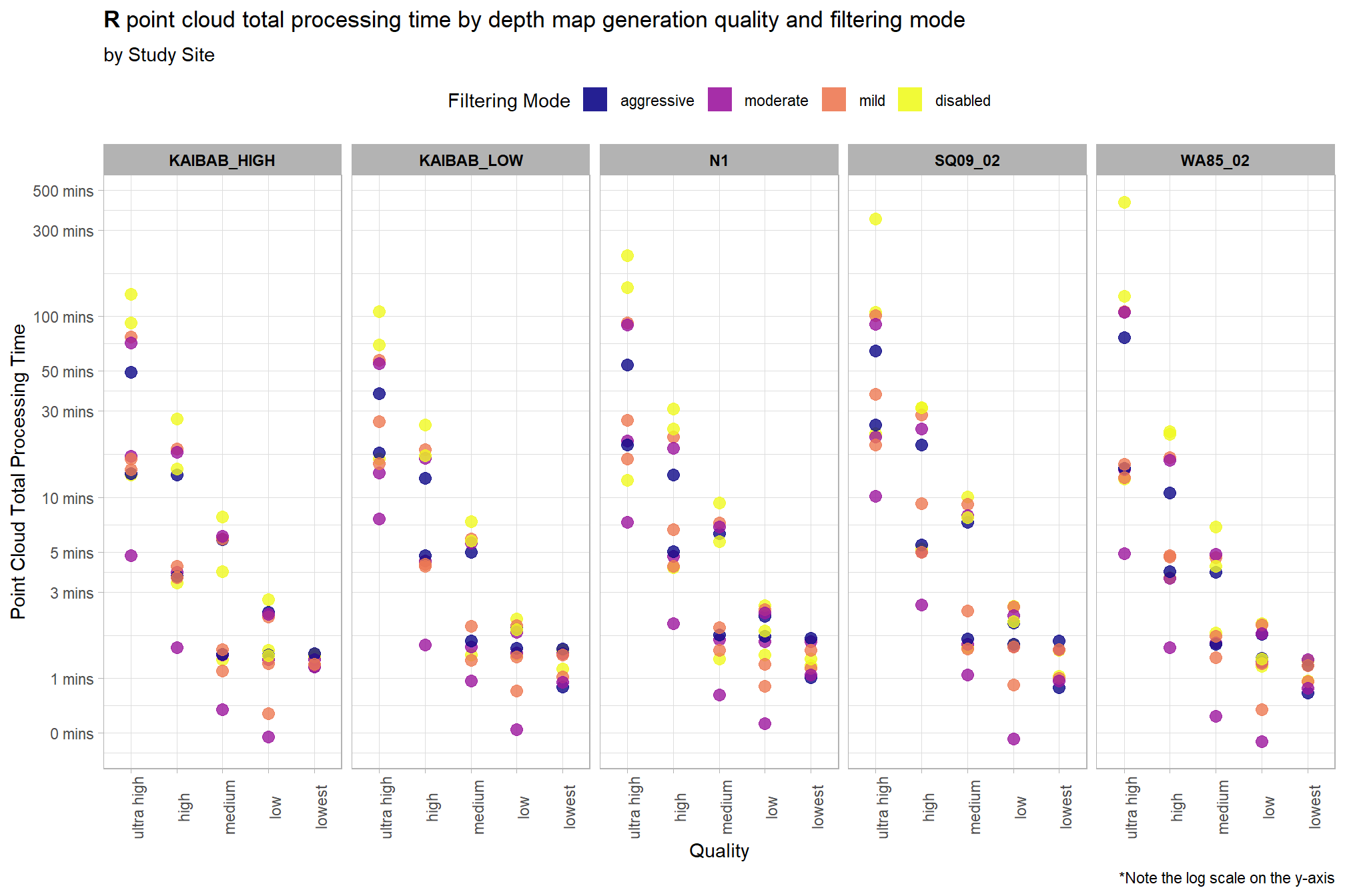
Notice there are some outlier study sites in the point cloud processing time

ptcld_processing_data %>% 
  ggplot(
    mapping = aes(
      y = timer_total_time_mins
      , x = depth_maps_generation_quality
      , color = depth_maps_generation_filtering_mode
    )
  ) +
  geom_point(size = 3, alpha = 0.8) +
  facet_grid(
    cols = vars(study_site)
    , labeller = label_wrap_gen(width = 35, multi_line = TRUE)
  ) +
  scale_color_viridis_d(option = "plasma") +
  scale_y_log10(
    labels = scales::comma_format(suffix = " mins", accuracy = 1)
    , breaks = scales::breaks_log(n = 9)
  ) +
  labs(
    color = "Filtering Mode"
    , y = "Point Cloud Total Processing Time"
    , x = "Quality"
    , title = bquote(
        bold("R") ~
        "point cloud total processing time by depth map generation quality and filtering mode"
    )
    , subtitle = "by Study Site"
    , caption = "*Note the log scale on the y-axis"
  ) +
  theme_light() + 
  theme(
    legend.position = "top"
    , legend.direction  = "horizontal"
    , strip.text = element_text(color = "black", face = "bold")
    , axis.text.x = element_text(angle = 90)
  ) +
  guides(
    color = guide_legend(override.aes = list(shape = 15, size = 6, alpha = 0.9))
  )

4.3.3 R Processing Time vs # Points

ptcld_processing_data %>% 
  ggplot(
    mapping = aes(
      x = number_of_points
      , y = timer_total_time_mins
    )
  ) +
  geom_point(alpha = 0.7, color = "navy") +
  scale_y_log10(
    labels = scales::comma_format(suffix = " mins", accuracy = 1)
    , breaks = scales::breaks_log(n = 9)
  ) +
  scale_x_log10(
    labels = scales::comma_format(suffix = " M", scale = 1e-6, accuracy = 1)
    , breaks = scales::breaks_log(n = 6)
  ) +
  labs(
    y = "Point Cloud Total Processing Time"
    , x = "Dense Point Cloud # Points"
    , title = bquote(
        bold("R") ~
        "point cloud total processing time versus dense point cloud number of points"
    )
    , caption = "*Note the log scale on both axes"
  ) +
  theme_light()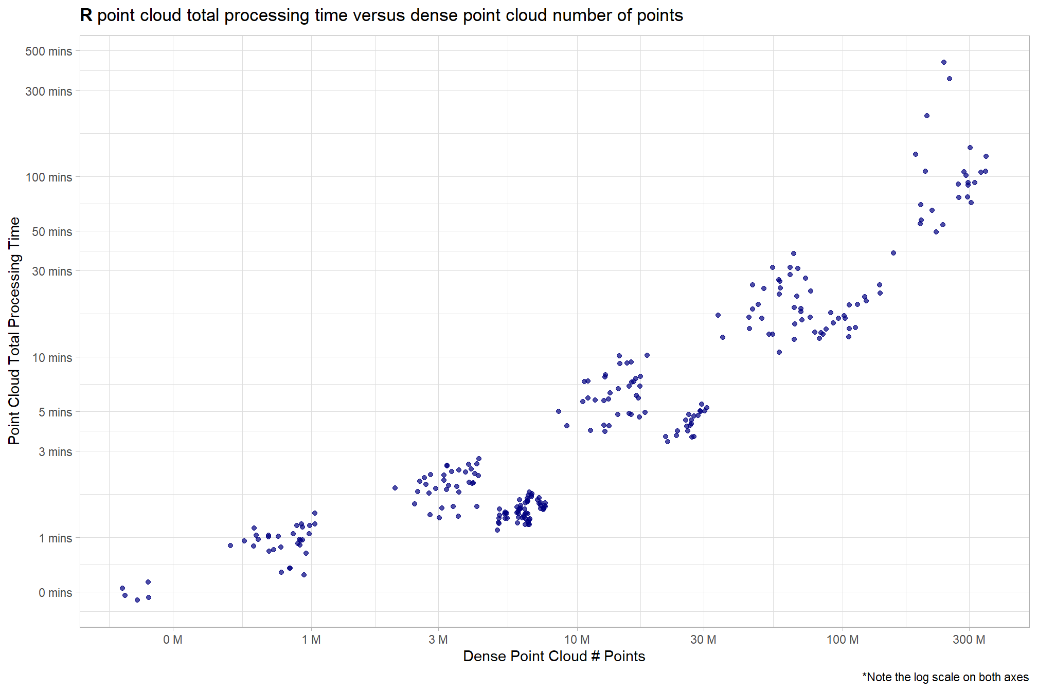

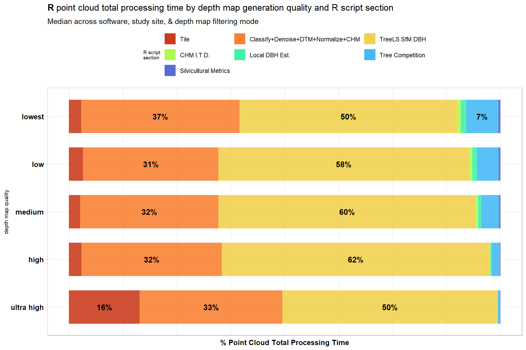
4.3.4 R Processing Section Timing

ptcld_processing_data %>% 
  dplyr::select(
    depth_maps_generation_quality
    , tidyselect::ends_with("_mins")
  ) %>% 
  dplyr::select(-c(timer_total_time_mins)) %>% 
  tidyr::pivot_longer(
    cols = -c(depth_maps_generation_quality)
    , names_to = "section"
    , values_to = "mins"
  ) %>% 
  # dplyr::count(depth_maps_generation_quality, section)
  dplyr::group_by(depth_maps_generation_quality, section) %>% 
  dplyr::summarise(med_mins = median(mins)) %>% 
  dplyr::group_by(depth_maps_generation_quality) %>% 
  dplyr::mutate(
    total_mins = sum(med_mins)
    , pct_mins = med_mins/total_mins 
  ) %>% 
  dplyr::ungroup() %>% 
  dplyr::mutate(
    section = section %>% 
      stringr::str_remove_all("timer_") %>% 
      stringr::str_remove_all("_time_mins") %>% 
      factor(
        ordered = T
        , levels = c(
          "tile"
          , "class_dtm_norm_chm"
          , "treels"
          , "itd"
          , "estdbh"
          , "competition"
          , "silv"
          ## olde
          # "tile"
          # , "denoise"
          # , "classify"
          # , "dtm"
          # , "normalize"
          # , "chm"
          # , "treels"
          # , "itd"
          # , "estdbh"
          # , "competition"
          # , "silv"
        )
        , labels = c(
          "Tile"
          , "Classify+Denoise+DTM+Normalize+CHM"
          , "TreeLS SfM DBH"
          , "CHM I.T.D."
          , "Local DBH Est."
          , "Tree Competition"
          , "Silvicultural Metrics"
        )
      ) %>% forcats::fct_rev()
  ) %>%
  
ggplot(
  mapping = aes(x = pct_mins, y = depth_maps_generation_quality, fill=section, group=section)
) +
  geom_col(
    width = 0.7, alpha=0.8
  ) +
  geom_text(
    mapping = aes(
        label = scales::percent(ifelse(pct_mins>=0.06,pct_mins,NA), accuracy = 1)
        , fontface = "bold"
      )
    , position = position_stack(vjust = 0.5)
    , color = "black", size = 4
  ) +
  scale_fill_viridis_d(option = "turbo", begin = 0.1, end = 0.9) +
  scale_x_continuous(labels = scales::percent_format()) +
  labs(
    fill = "R script\nsection"
    , y = "depth map quality"
    , x = "% Point Cloud Total Processing Time"
    , title = bquote(
        bold("R") ~
        "point cloud total processing time by depth map generation quality and R script section"
    )
    , subtitle = "Median across software, study site, & depth map filtering mode "
  ) +
  theme_light() +
  theme(
    legend.position = "top"
    , legend.direction  = "horizontal"
    , legend.title = element_text(size=7)
    , axis.title.x = element_text(size=10, face = "bold")
    , axis.title.y = element_text(size = 8)
    , axis.text.x = element_blank()
    , axis.text.y = element_text(color = "black",size=10, face = "bold")
    , axis.ticks.x = element_blank()
  ) +
  guides(
    fill = guide_legend(nrow = 3, byrow = T, reverse = T, override.aes = list(alpha = 0.9))
  )  

ggplot2::ggsave("../data/processing_time_brkdown.png", width = 8.5, height = 6)

4.3.5 Summary of point cloud data

Use flight boundary to calculate the per ha metrics but all of the flight boundaries based on the SfM data are different ; so will just use the Metashape “high” quality area median across filtering modes applied to all.

4.3.5.1 Table

table_temp =
  ptcld_processing_data %>% 
  dplyr::select(
    # unique vars
    software, tidyselect::starts_with("depth_maps"), study_site
    # vars
    , number_of_points, timer_total_time_mins
  ) %>% 
  # add area
  dplyr::inner_join(
    ptcld_processing_data %>% 
      dplyr::mutate(
        las_area_m2 = dplyr::case_when(
          tolower(software)=="metashape"
            & tolower(depth_maps_generation_quality)=="high" ~ las_area_m2
          , T ~ NA
        )
      ) %>% 
      dplyr::group_by(study_site) %>% 
      dplyr::summarise(las_area_m2 = median(las_area_m2, na.rm = T))
    , by = "study_site"
  ) %>% 
  # calculate per area metrics
  dplyr::mutate(
    number_of_points_m2 = number_of_points/las_area_m2
    , timer_total_time_mins_ha = timer_total_time_mins/(las_area_m2/10000)
  ) %>%
  # summary
  dplyr::rename_with(
    .fn = function(x){
      x %>% 
      stringr::str_replace_all("depth_maps_generation_quality", "quality") %>% 
      stringr::str_replace_all("depth_maps_generation_filtering_mode", "filtering")
    }
  ) %>% 
  # plot it?
  # ggplot(mapping = aes(fill = software)) +
  #   geom_boxplot(mapping = aes(x = software, y = timer_total_time_mins_ha)) + 
  #   facet_wrap(facets = vars(quality, filtering), ncol = 10) +
  #   scale_fill_viridis_d(option = "rocket", begin = 0.3, end = 0.9, drop = F) +
  #   scale_y_log10(
  #     labels = scales::comma_format(suffix = " mins", accuracy = 0.1)
  #     , breaks = scales::breaks_log(n = 9)
  #   ) +
  #   theme_light() 
  # or table it
  dplyr::group_by(software, quality, filtering) %>% 
  dplyr::summarise(
    dplyr::across(
      c(number_of_points_m2, timer_total_time_mins_ha)
      , .fns = list(mean = mean, sd = sd)
    )
    , n = dplyr::n()
  ) %>% 
  # combine mean/sd
  dplyr::mutate(
    pts = paste0(
      number_of_points_m2_mean %>% 
        round(1) %>% 
        scales::comma(accuracy = 1)
      , "<br>("
      , number_of_points_m2_sd %>% 
          round(1) %>% 
          scales::comma(accuracy = 1)
      , ")"
    )
    , mins = paste0(
      timer_total_time_mins_ha_mean %>% round(1) %>% scales::comma(accuracy = 0.1)
      , "<br>("
      , timer_total_time_mins_ha_sd %>% round(1) %>% scales::comma(accuracy = 0.1)
      , ")"
    )
  ) %>% 
  dplyr::ungroup() %>% 
  select(software,quality,filtering,pts,mins)
table_temp =
  dplyr::bind_rows(
    table_temp %>% dplyr::select(-c(mins)) %>% tidyr::pivot_wider(names_from = filtering, values_from = pts) %>% 
      dplyr::mutate(metric = "Points m<sup>-2</sup>")
    , table_temp %>% dplyr::select(-c(pts)) %>% tidyr::pivot_wider(names_from = filtering, values_from = mins) %>% 
      dplyr::mutate(metric = "Processing time<br>mins ha<sup>-1</sup>")
  ) %>% 
  dplyr::relocate(software) %>% 
  dplyr::relocate(metric)
# table
table_temp %>% 
  kableExtra::kbl(escape = F) %>% 
  kableExtra::kable_styling() %>% 
  kableExtra::collapse_rows(columns = 1:2, valign = "top")

metric	software	quality	aggressive	moderate	mild	disabled
Points m-2	METASHAPE	ultra high	3,546 (1,444)	4,446 (1,687)	4,544 (1,801)	4,597 (1,786)
		high	789 (296)	972 (345)	1,019 (378)	1,028 (377)
		medium	183 (64)	224 (76)	238 (84)	239 (84)
		low	43 (13)	52 (17)	57 (19)	57 (20)
		lowest	11 (3)	12 (4)	13 (4)	13 (4)
	OPENDRONEMAP	ultra high	1,684 (664)	1,678 (603)	1,557 (515)	1,455 (566)
		high	421 (125)	421 (128)	418 (134)	418 (133)
		medium	100 (32)	100 (32)	99 (33)	100 (34)
		low	99 (32)	100 (33)	99 (33)	100 (33)
		lowest	99 (31)	100 (33)	100 (32)	99 (33)
	PIX4D	ultra high	NA	262 (84)	934 (317)	3,454 (1,185)
		high	NA	58 (24)	217 (90)	774 (318)
		medium	NA	14 (4)	54 (16)	193 (60)
		low	NA	4 (1)	13 (4)	47 (14)
Processing time mins ha-1	METASHAPE	ultra high	9.1 (4.4)	13.3 (6.1)	14.0 (6.2)	17.5 (8.2)
		high	2.2 (0.8)	2.9 (0.9)	3.2 (1.2)	4.3 (1.2)
		medium	0.9 (0.3)	1.0 (0.3)	1.0 (0.4)	1.3 (0.4)
		low	0.3 (0.1)	0.3 (0.1)	0.3 (0.1)	0.4 (0.1)
		lowest	0.1 (0.0)	0.2 (0.0)	0.2 (0.0)	0.2 (0.0)
	OPENDRONEMAP	ultra high	2.8 (1.1)	2.7 (1.0)	2.4 (0.7)	2.4 (0.9)
		high	0.7 (0.2)	0.7 (0.2)	0.7 (0.2)	0.6 (0.2)
		medium	0.2 (0.1)	0.2 (0.1)	0.2 (0.1)	0.2 (0.1)
		low	0.2 (0.1)	0.2 (0.1)	0.2 (0.1)	0.2 (0.0)
		lowest	0.2 (0.1)	0.2 (0.1)	0.2 (0.1)	0.2 (0.0)
	PIX4D	ultra high	NA	1.1 (0.4)	3.8 (1.7)	42.1 (31.0)
		high	NA	0.3 (0.1)	0.9 (0.5)	3.5 (1.6)
		medium	NA	0.1 (0.0)	0.3 (0.1)	0.8 (0.3)
		low	NA	0.1 (0.0)	0.1 (0.0)	0.3 (0.1)

4.3.6 R Processing Summary

table_temp = ptcld_processing_data %>% 
  dplyr::select(
    # unique vars
    software, tidyselect::starts_with("depth_maps"), study_site
    # vars
    , number_of_points, timer_total_time_mins
  ) %>% 
  # add area
  dplyr::inner_join(
    ptcld_processing_data %>% 
      dplyr::mutate(
        las_area_m2 = dplyr::case_when(
          tolower(software)=="metashape"
            & tolower(depth_maps_generation_quality)=="high" ~ las_area_m2
          , T ~ NA
        )
      ) %>% 
      dplyr::group_by(study_site) %>% 
      dplyr::summarise(las_area_m2 = median(las_area_m2, na.rm = T))
    , by = "study_site"
  ) %>% 
  # calculate per area metrics
  dplyr::mutate(
    number_of_points_m2 = number_of_points/las_area_m2
    , timer_total_time_mins_ha = timer_total_time_mins/(las_area_m2/10000)
  ) %>%
  # summary
  dplyr::rename_with(
    .fn = function(x){
      x %>% 
      stringr::str_replace_all("depth_maps_generation_quality", "quality") %>% 
      stringr::str_replace_all("depth_maps_generation_filtering_mode", "filtering")
    }
  ) 

# plot it?
p1_temp =
  table_temp %>% 
  dplyr::mutate(quality = forcats::fct_rev(quality)) %>% 
  ggplot(mapping = aes(x = filtering, y = timer_total_time_mins_ha, fill = software)) +
    geom_point(
      mapping = aes(group=software, color = software)
      , position = position_nudge(x = -0.4)
      , alpha = 0.8
      , shape = "-", size = 5
    ) +
    geom_boxplot(
      width = 0.7, alpha = 0.8
      , position = position_dodge2(preserve = "single")
      , outliers = F
    ) +
    # set vertical lines between x groups
    geom_vline(xintercept = seq(0.5, length(table_temp$filtering), by = 1), color="gray22", lwd=.5) +
    facet_grid(cols = vars(quality)) +
    scale_fill_viridis_d(option = "rocket", begin = 0.3, end = 0.9, drop = F) +
    scale_color_viridis_d(option = "rocket", begin = 0.3, end = 0.9, drop = F) +
    scale_y_log10(
      labels = scales::comma_format(suffix = " mins", accuracy = 0.1)
      , breaks = scales::breaks_log(n = 9)
    ) +
    labs(
      subtitle = "quality"
      , y = latex2exp::TeX("Pt. Cld. Processing Time (mins $\\cdot ha^{-1}$)")
      , x = "filtering mode"
    ) +
    theme_light() +
    theme(
      legend.position = "bottom"
      , legend.direction  = "horizontal"
      , panel.grid.major.x = element_blank()
      , panel.grid.minor.x = element_blank()
      , axis.text.x = element_text(angle = 90, vjust = 0.5, hjust = 1, size = 7)
      , strip.text = element_text(color = "black", face = "bold")
      , plot.subtitle = element_text(hjust = 0.5)
    ) +
    guides(
      fill = guide_legend(reverse = T, override.aes = list(alpha = 1, color = NA, shape = NA, lwd = NA))
      , color = "none"
    )
# plot it?
p2_temp =
  table_temp %>% 
  dplyr::mutate(quality = forcats::fct_rev(quality)) %>% 
  ggplot(mapping = aes(x = filtering, y = number_of_points_m2, fill = software)) +
    geom_point(
      mapping = aes(group=software, color = software)
      , position = position_nudge(x = -0.4)
      , alpha = 0.8
      , shape = "-", size = 5
    ) +
    geom_boxplot(
      width = 0.7, alpha = 0.8
      , position = position_dodge2(preserve = "single")
      , outliers = F
    ) +
    # set vertical lines between x groups
    geom_vline(xintercept = seq(0.5, length(table_temp$filtering), by = 1), color="gray22", lwd=.5) +
    facet_grid(cols = vars(quality)) +
    scale_fill_viridis_d(option = "rocket", begin = 0.3, end = 0.9, drop = F) +
    scale_color_viridis_d(option = "rocket", begin = 0.3, end = 0.9, drop = F) +
    scale_y_log10(
      labels = scales::comma_format(accuracy = 1)
      , breaks = scales::breaks_log(n = 9)
    ) +
    labs(
      subtitle = "quality"
      , y = latex2exp::TeX("Point Density (points $\\cdot m^{-2}$)")
      , x = "filtering mode"
    ) +
    theme_light() +
    theme(
      legend.position = "bottom"
      , legend.direction  = "horizontal"
      , panel.grid.major.x = element_blank()
      , panel.grid.minor.x = element_blank()
      , axis.text.x = element_text(angle = 90, vjust = 0.5, hjust = 1, size = 7)
      , strip.text = element_text(color = "black", face = "bold")
      , plot.subtitle = element_text(hjust = 0.5)
    ) +
    guides(
      fill = guide_legend(reverse = T, override.aes = list(alpha = 1, color = NA, shape = NA, lwd = NA))
      , color = "none"
    )
# combine plots
p2_temp / p1_temp + patchwork::plot_layout(guides = "collect") & theme(legend.position = "bottom")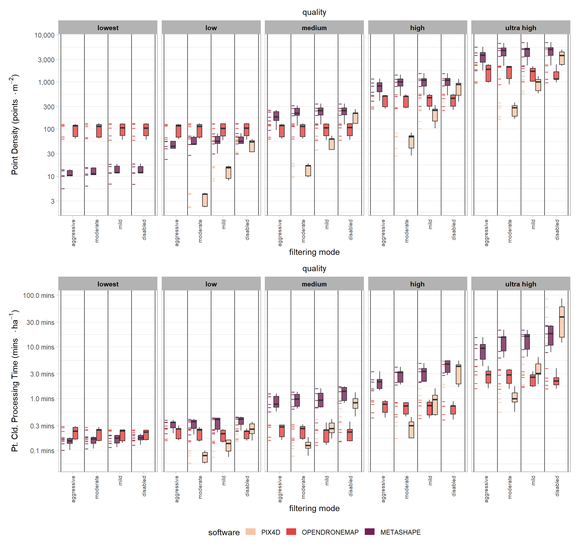

ggplot2::ggsave("../data/ptcld_summary_stats.png", height = 8.5, width = 11)

4.3.7 SfM image processing time summary

Because the SfM photogrammetry software were each run on different processing computers we need to normalize the processing time by software. SfM image processing time was normalized using Min-Max normalization as:

\[ x^{\prime}_{ij} = \frac{x_{ij}-x_{min[j]}}{x_{max[j]}-x_{min[j]}} \]

where \(i\) is the the study site observation within each software \(j\) where each software was implemented on a different computer.

ptcld_processing_data %>%
  dplyr::group_by(software, depth_maps_generation_quality, depth_maps_generation_filtering_mode) %>% 
  dplyr::mutate(med = median(total_sfm_time_norm, na.rm = T)) %>% 
  dplyr::ungroup() %>% 
  dplyr::mutate(depth_maps_generation_quality = forcats::fct_rev(depth_maps_generation_quality)) %>%
  ggplot(mapping = aes(
    x = depth_maps_generation_filtering_mode
    , y = total_sfm_time_norm
    , fill = med
  )) +
    geom_boxplot(width = 0.7, outliers = F, fill = "slategray") +
    facet_grid(
      rows = vars(software)
      , cols = vars(depth_maps_generation_quality)
    ) +
    scale_fill_viridis_c(option = "mako", direction = -1, end = 0.9) +
    scale_y_continuous(
      limits = c(-0.02,1.02)
      , breaks = c(0, 1)
      , minor_breaks = seq(0.2,0.8,0.2)
      , labels = c("min","max")
    ) +
    labs(x = "filtering mode", y = "SfM Image Processing Time (normalized)",subtitle = "quality") + 
    theme_light() +
    theme(
      legend.position = "none"
      , legend.direction  = "horizontal"
      , panel.grid.major.x = element_blank()
      , panel.grid.minor.x = element_blank()
      , panel.grid.major.y = element_line(color = "black")
      , axis.ticks.y = element_blank()
      , axis.text.x = element_text(angle = 90, vjust = 0.5, hjust = 1)
      , strip.text = element_text(color = "black", face = "bold")
      , plot.subtitle = element_text(hjust = 0.5)
    )

ggplot2::ggsave("../data/sfm_img_processing_time.png", height = 7, width = 10.5)

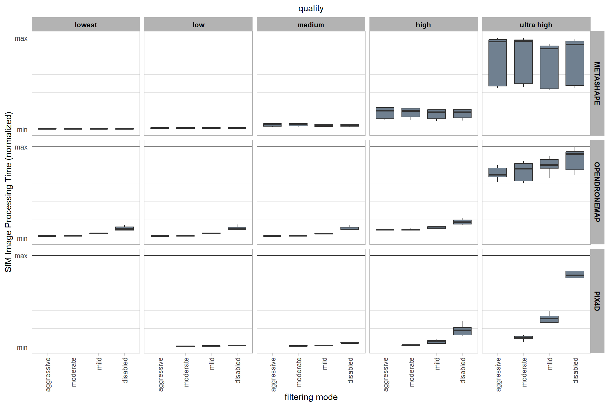
table it

table_temp =
  ptcld_processing_data %>% 
  dplyr::group_by(software, depth_maps_generation_quality, depth_maps_generation_filtering_mode) %>%
  dplyr::summarise(
    dplyr::across(
      total_sfm_time_norm
      , .fns = list(mean = mean, sd = sd, min = min, max = max)
    )
    , n = dplyr::n()
  ) %>% 
  dplyr::mutate(
    range = paste0(
      total_sfm_time_norm_min %>% scales::number(accuracy = 0.01)
      , "—"
      , total_sfm_time_norm_max %>% scales::number(accuracy = 0.01)
    )
    , depth_maps_generation_quality = depth_maps_generation_quality %>% forcats::fct_rev()
  ) %>% 
  select(-c(n,total_sfm_time_norm_min, total_sfm_time_norm_max)) %>% 
  dplyr::ungroup() %>% 
  dplyr::arrange(software, depth_maps_generation_quality, depth_maps_generation_filtering_mode)

table_temp %>% 
  # dplyr::select(-c(software)) %>% 
  kableExtra::kbl(
    digits = 2
    , caption = "Normalized SfM Image Processing Time"
    , col.names = c(
      "software", "quality", "filtering mode"
      , "Mean"
      , "Std Dev", "Range"
    )
    , escape = F
  ) %>% 
  kableExtra::kable_styling() %>% 
  # kableExtra::pack_rows(index = table(forcats::fct_inorder(table_temp$software))) %>% 
  kableExtra::collapse_rows(columns = 1:2, valign = "top") %>%
  kableExtra::scroll_box(height = "8in")

Table 4.1: Normalized SfM Image Processing Time

software	quality	filtering mode	Mean	Std Dev	Range
METASHAPE	lowest	aggressive	0.00	0.00	0.00—0.01
		moderate	0.00	0.00	0.00—0.01
		mild	0.00	0.00	0.00—0.01
		disabled	0.00	0.00	0.00—0.01
	low	aggressive	0.01	0.01	0.00—0.02
		moderate	0.01	0.01	0.00—0.02
		mild	0.01	0.01	0.00—0.02
		disabled	0.01	0.01	0.00—0.02
	medium	aggressive	0.04	0.02	0.02—0.06
		moderate	0.04	0.02	0.02—0.06
		mild	0.04	0.02	0.02—0.05
		disabled	0.04	0.02	0.02—0.06
	high	aggressive	0.18	0.07	0.10—0.24
		moderate	0.18	0.06	0.10—0.23
		mild	0.16	0.06	0.09—0.21
		disabled	0.17	0.06	0.09—0.22
	ultra high	aggressive	0.77	0.29	0.45—1.00
		moderate	0.78	0.28	0.46—1.00
		mild	0.72	0.26	0.43—0.93
		disabled	0.76	0.27	0.45—0.99
OPENDRONEMAP	lowest	aggressive	0.02	0.00	0.02—0.02
		moderate	0.02	0.01	0.00—0.03
		mild	0.05	0.00	0.04—0.05
		disabled	0.11	0.02	0.08—0.14
	low	aggressive	0.02	0.00	0.02—0.03
		moderate	0.03	0.00	0.02—0.03
		mild	0.05	0.01	0.04—0.06
		disabled	0.11	0.03	0.08—0.15
	medium	aggressive	0.02	0.00	0.02—0.02
		moderate	0.02	0.00	0.02—0.03
		mild	0.05	0.00	0.04—0.05
		disabled	0.11	0.02	0.09—0.14
	high	aggressive	0.09	0.01	0.08—0.10
		moderate	0.09	0.01	0.08—0.10
		mild	0.12	0.01	0.10—0.13
		disabled	0.18	0.03	0.14—0.22
	ultra high	aggressive	0.71	0.08	0.61—0.80
		moderate	0.73	0.11	0.60—0.85
		mild	0.79	0.09	0.66—0.90
		disabled	0.86	0.13	0.69—1.00
PIX4D	low	moderate	0.00	0.00	0.00—0.01
		mild	0.01	0.00	0.01—0.01
		disabled	0.01	0.01	0.01—0.02
	medium	moderate	0.01	0.01	0.00—0.02
		mild	0.02	0.00	0.01—0.02
		disabled	0.04	0.01	0.02—0.05
	high	moderate	0.02	0.01	0.01—0.03
		mild	0.06	0.02	0.03—0.08
		disabled	0.18	0.07	0.12—0.28
	ultra high	moderate	0.10	0.03	0.05—0.12
		mild	0.29	0.09	0.15—0.39
		disabled	0.78	0.17	0.54—1.00