Section 4 Point Cloud Processing and Pile Segmentation
We’ll use the point cloud data alone (to begin with) to attempt to classify slash piles without additional spectral information.
We’ll use the cloud2trees package to perform all preprocessing of point cloud data which includes:
- ground classification and noise removal
- raster data (DTM and CHM) generation
- point cloud height normalization
All of this can be accomplished using the cloud2raster() function. After generating these products from the raw point cloud we’ll perform object segmentation to attempt to detect round, conical objects like slash piles from: 1) the normalized point cloud directly; 2) the CHM which we’ll generate by setting the minimum height to zero (essentially a digital surface model [DSM] with the ground removed).
To attempt to identify slash piles from the CHM/DSM, we can use watershed segmentation (potentially without “seed” points) in a bottom-up approach. Insert something from paper about bottom-up approach that uses a CHM “slice” near the ground. For slash piles, which are often irregular and may not have a distinct “treetop” equivalent, CHM-based methods might be less directly applicable unless the piles present a very clear, isolated conical or rounded form. Could use expected morphology of the slash piles (e.g. maximum height) based on prior research.
To attempt to detect slash piles directly from the point cloud we can use a clustering algorithm such as DBSCAN (Density-Based Spatial Clustering of Applications with Noise) which identifies clusters based on point density, making it effective for detecting clusters of arbitrary shapes and sizes. It does not require the number of clusters to be specified beforehand. Fu et al. (2022) outline a method using DBSCAN in semi-automated way to segment individual trees from TLS data. After segmenting the point cloud using DBSCAN, either random forest can be used as a classifier (i.e. classification step) or a rules-based method can filter segments to distinguish slash piles from other objects based on their extracted geometric features. The general workflow is:
- for each point in the normalized non-ground point cloud, compute a suite of relevant geometric features within a defined local neighborhood radius using
lidR::point_metrics() - calculate features derived from PCA, such as linearity, planarity, sphericity, and surface variation. Also, compute curvature (mean, Gaussian) and roughness
- perform object segmentation/clustering to group points belonging to individual objects using DBSCAN which can identify dense clusters without requiring a predefined number of objects 4a) classify the segmented objects (clusters) as “slash pile” or “non-slash pile” based on their extracted features (e.g., sphericity, roughness, height, volume) with a random forest classifier using a manually annotated subset of segmented objects 4b) or used a rules-based approach to filter the segmented objects based on their extracted features (e.g., sphericity, roughness, height, volume) based on expected morphology of the slash piles (e.g. maximum height) using prior research or prescription settings.
- merge small, adjacent segments that likely belong to a single slash pile based on proximity and connectivity
- perform a confusion matrix-based evaluation on the results
- Section 5 builds and tests a raster-based watershed segmentation methodology
- Section 6 (under development) combines the raster-based watershed segmentation methodology with spectral information in a data fusion approach
4.1 Process Raw Point Cloud
We’ll use cloud2trees::cloud2raster() to process the raw point cloud data
if(!dir.exists("../data/point_cloud_processing_delivery")){
  cloud2raster_ans <- cloud2trees::cloud2raster(
    output_dir = "../data"
    , input_las_dir = "f:\\PFDP_Data\\p4pro_images\\P4Pro_06_17_2021_half_half_optimal\\2_densification\\point_cloud"
    , accuracy_level = 2
    , keep_intrmdt = T
    , dtm_res_m = 0.25
    , chm_res_m = 0.1
    , min_height = 0 # effectively generates a DSM based on non-ground points
  )
}else{
  # dtm_temp <- terra::rast("../data/point_cloud_processing_delivery/dtm_0.25m.tif")
  # chm_temp <- terra::rast("../data/point_cloud_processing_delivery/chm_0.1m.tif")

  dtm_temp <- terra::rast("../data/xxpoint_cloud_processing_delivery/dtm_0.5m.tif")
  chm_temp <- terra::rast("../data/xxpoint_cloud_processing_delivery/chm_0.2m.tif")

  cloud2raster_ans <- list(
    "dtm_rast" = dtm_temp
    , "chm_rast" = chm_temp
  )
}
let’s check out the DTM
cloud2raster_ans$dtm_rast %>%
  terra::aggregate(fact = 2) %>%  #, fun = "median", cores = lasR::half_cores(), na.rm = T) %>%
  terra::plot(axes = F)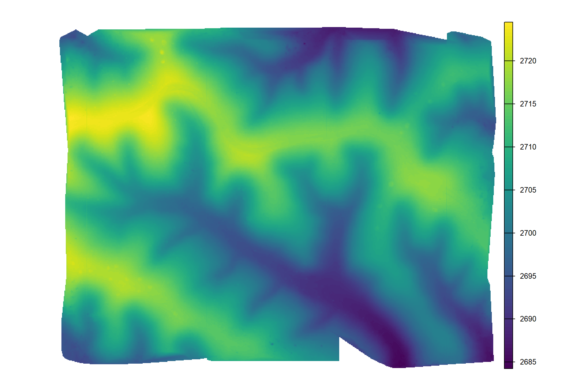
and CHM
cloud2raster_ans$chm_rast %>%
  terra::aggregate(fact = 2) %>%  #, fun = "median", cores = lasR::half_cores(), na.rm = T) %>%
  terra::plot(col = viridis::plasma(100), axes = F)
## |---------|---------|---------|---------|========================================= 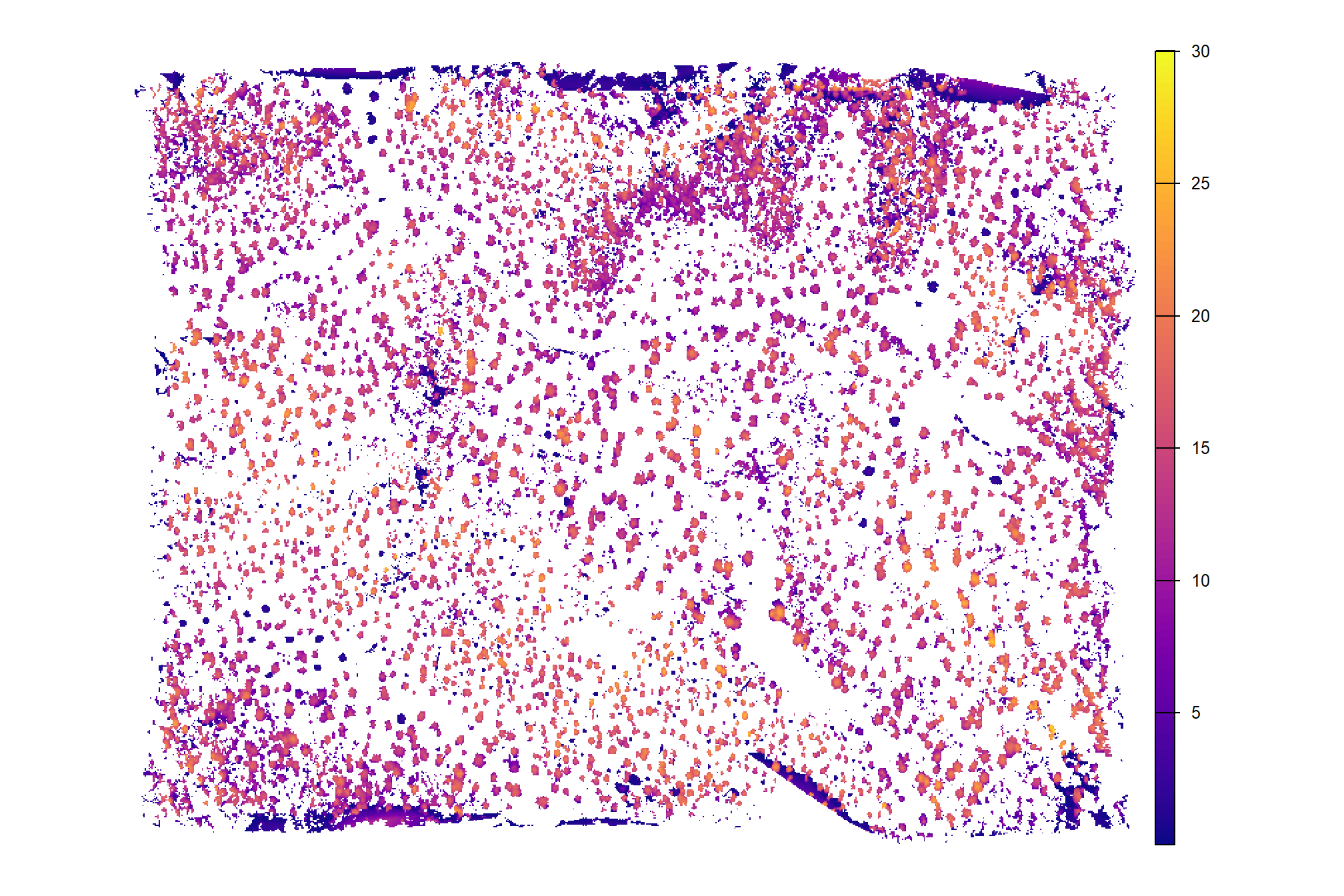
4.1.1 DTM and CHM + piles
let’s visually inspect the DTM and CHM with the pile outlines overlaid
p_fn_temp <- function(
    rn
    , df = slash_piles_polys
    , rast = cloud2raster_ans$dtm_rast
    , crs = terra::crs(cloud2raster_ans$dtm_rast)
    , my_title = ""
    , vopt = "viridis"
    , lim = NULL
) {
  # scale the buffer based on the largest
    d_temp <- df %>%
      dplyr::arrange(tolower(comment), desc(diameter)) %>%
      dplyr::slice(rn) %>%
      sf::st_transform(crs)

    # plt classifier
    # convert to stars
    comp_st <- rast %>%
      terra::crop(
        d_temp %>% sf::st_buffer(20) %>% terra::vect()
      ) %>%
      terra::as.data.frame(xy = T) %>%
      dplyr::rename(f=3)

    # ggplot
    comp_temp <- ggplot2::ggplot() +
      ggplot2::geom_tile(data = comp_st, ggplot2::aes(x=x,y=y,fill=f)) +
      ggplot2::geom_sf(data = d_temp, fill = NA, color = "gray33", lwd = 0.4) +
      ggplot2::scale_x_continuous(expand = c(0, 0)) +
      ggplot2::scale_y_continuous(expand = c(0, 0)) +
      ggplot2::labs(
        x = ""
        , y = ""
        , subtitle = my_title
      ) +
      ggplot2::theme_void() +
      ggplot2::theme(
        legend.position = "none" # c(0.5,1)
        , legend.margin = margin(0,0,0,0)
        , legend.text = element_text(size = 8)
        , legend.title = element_text(size = 8)
        , legend.key = element_rect(fill = "white")
        # , plot.title = ggtext::element_markdown(size = 10, hjust = 0.5)
        , plot.title = element_text(size = 8, hjust = 0.5, face = "bold")
        , plot.subtitle = element_text(size = 6, hjust = 0.5, face = "italic")
      )
  if(!is.null(lim)){
    comp_temp <- comp_temp +
      ggplot2::scale_fill_viridis_c(option = vopt, limits = lim)
  }else{
    comp_temp <- comp_temp +
      ggplot2::scale_fill_viridis_c(option = vopt)
  }

  plt_temp <- comp_temp
  return(list("plt"=plt_temp,"d"=d_temp))
}

# p_fn_temp(
#   rn = 5
#   # , lim = c(floor(terra::minmax(cloud2raster_ans$dtm_rast)[1]*0.98), floor(terra::minmax(cloud2raster_ans$dtm_rast)[2]*1.02))
# )
# p_fn_temp(
#   rn = 11
#   , rast = cloud2raster_ans$chm_rast
#   , vopt = "plasma"
# )
# combine 3
plt_combine_temp <- function(
    rn
    , df = slash_piles_polys %>% dplyr::filter(!is.na(comment))
    , rast1 = cloud2raster_ans$dtm_rast
    , title1 = "DTM"
    , vopt1 = "viridis"
    , rast2 = cloud2raster_ans$chm_rast
    , title2 = "CHM"
    , vopt2 = "plasma"
    , crs = terra::crs(cloud2raster_ans$dtm_rast)
) {
  # composite 1
  ans1 <- p_fn_temp(
    rn = rn
    , df = df
    , rast = rast1
    , my_title = title1
    , crs = crs
    , vopt = vopt1
  )
  # composite 2
  ans2 <- p_fn_temp(
    rn = rn
    , df = df
    , rast = rast2
    , my_title = title2
    , crs = crs
    , vopt = vopt2
  )
  # plt rgb
    rgb_temp <-
      ortho_plt_fn(ans1$d) +
      ggplot2::geom_sf(data = ans1$d, fill = NA, color = "white", lwd = 0.3)
  # combine
    r <- ans1$plt + ans2$plt + rgb_temp
    return(r)
}

# plt_combine_temp(2)

# add pile locations
plt_list_rast_comp <- sample(1:nrow(slash_piles_polys %>% dplyr::filter(!is.na(comment))),10) %>%
  purrr::map(plt_combine_temp)
# plt_list_rast_comp[[2]]
combine the plots for a few piles
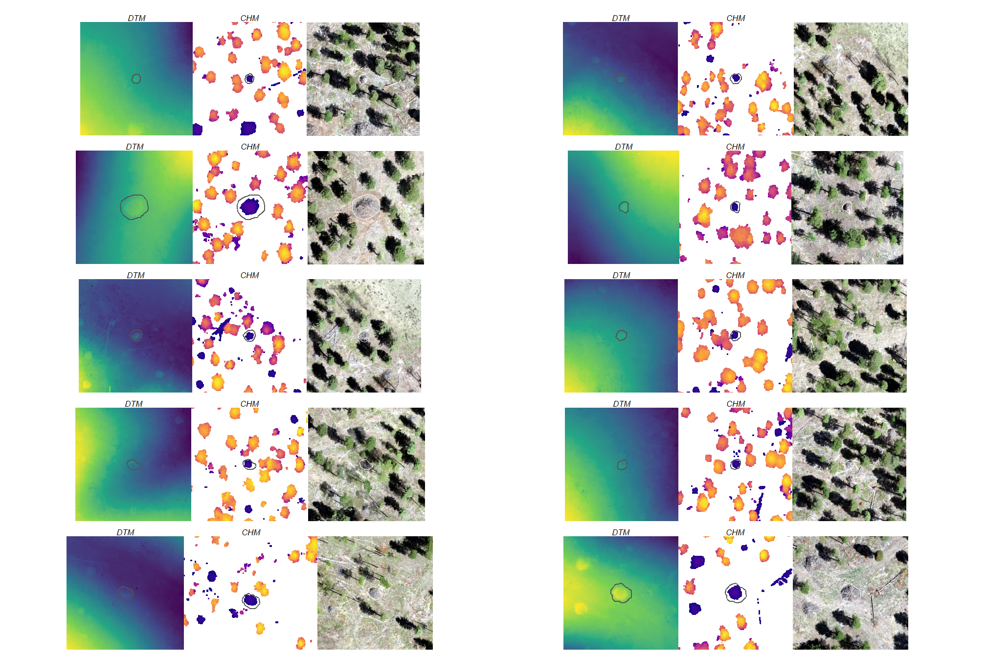
a few things are noteworthy in these examples:
- Piles are clearly visible in some areas of the DTM but less visible in other areas
- Piles are delineated in the CHM but with varying degrees of definition based on surrounding terrain and pile structure
- The DTM and CHM were rarely impacted by shadows in the RGB imagery
- It is interesting to see coarse woody debris occasionally visible in the CHM