Chapter 4 Multilevel linear models: varying slopes, non-nested models, and other complexities (Ch 13)

This chapter starts on page 279

4.1 Setup

# bread-and-butter
library(tidyverse)
library(lubridate)
library(viridis)
library(scales)
library(latex2exp)
# visualization
library(cowplot)
library(kableExtra)
# Linear Mixed-Effects Models 
library(lme4)
library(broom.mixed)
# jags and bayesian
library(rjags)
library(MCMCvis)
library(HDInterval)
library(monomvn)
#set seed
set.seed(11)

4.2 Load data

# load individual, house-level observations
# srrs2 <- read.table("http://www.stat.columbia.edu/~gelman/arm/examples/radon/srrs2.dat", header=TRUE, sep=",") %>% 
srrs2 <- read.table("../data/radon/srrs2.dat", header=TRUE, sep=",") %>% 
  dplyr::mutate(
    fullfips = stfips*1000 + cntyfips
  )
# load county data
# cty <- read.table("http://www.stat.columbia.edu/~gelman/arm/examples/radon/cty.dat", header=TRUE, sep=",") %>% 
cty <- read.table("../data/radon/cty.dat", header=TRUE, sep=",") %>% 
  dplyr::mutate(fullfips = stfips*1000 + ctfips) %>% 
  # there are duplicates in this data
  dplyr::group_by(fullfips) %>% 
  dplyr::filter(dplyr::row_number()==1) %>% 
  dplyr::ungroup() %>% 
  dplyr::mutate(u = log(Uppm))
# join to individual, house radon measurement data
srrs2 <- srrs2 %>% 
  dplyr::left_join(cty %>% dplyr::select(fullfips, u), by = c("fullfips"="fullfips"))
# filter MN and create vars
radon_mn <- srrs2 %>% 
  dplyr::filter(
    state=="MN"
  ) %>% 
  dplyr::mutate(
    radon = activity
    , log.radon = log(ifelse(radon==0, .1, radon))
    , y = log.radon
    , x = floor # 0 for basement, 1 for first floor
    , county_index = as.numeric(as.factor(county))
  )
# unique uranium by county index 1:85
u <- radon_mn %>% 
  dplyr::group_by(county_index) %>% 
  summarize(u = dplyr::first(u)) %>% 
  ungroup() %>% 
  dplyr::arrange(county_index)

4.3 Varying intercepts and slopes (p. 279)

The next step in multilevel modeling is to allow more than one regression coefficient to vary by group. We shall illustrate with the radon model from the previous chapter, which is relatively simple because it only has a single individual-level predictor, \(x\) (the indicator for whether the measurement was taken on the first floor). We begin with a varying-intercept, varying-slope model including \(x\) but without the county-level uranium predictor; thus,

\[\begin{align*} y_i &\sim \textrm{N}(\alpha_{j[i]} + \beta_{j[i]} \cdot x_i, \sigma^2_y) \\ &\textrm{for} \; i = 1, \cdots, n \\ \left(\begin{array}{c} \alpha_{j}\\ \beta_{j} \end{array}\right) &\sim \textrm{N}\left(\left(\begin{array}{c} \mu_\alpha\\ \mu_\beta \end{array}\right) , \left(\begin{array}{cc} \sigma^{2}_{\alpha} & \rho\sigma_{\alpha}\sigma_{\beta}\\ \rho\sigma_{\alpha}\sigma_{\beta} & \sigma^{2}_{\beta} \end{array}\right) \right) \\ &\textrm{for} \; j = 1, \cdots, J \end{align*}\]

with variation in the \(\alpha_{j}\)’s and the \(\beta_{j}\)’s and also a between-group correlation parameter \(\rho\)

4.3.1 Using `lme4::lmer` (p. 279)

## Varying intercept & slopes w/ no group level predictors
M3 <- lme4::lmer(data = radon_mn, formula = y ~ x + (1 + x | county))
summary(M3)

Linear mixed model fit by REML [‘lmerMod’] Formula: y ~ x + (1 + x | county) Data: radon_mn

REML criterion at convergence: 2168.3

Scaled residuals: Min 1Q Median 3Q Max -4.4044 -0.6224 0.0138 0.6123 3.5682

Random effects: Groups Name Variance Std.Dev. Corr county (Intercept) 0.1216 0.3487
x 0.1181 0.3436 -0.34 Residual 0.5567 0.7462
Number of obs: 919, groups: county, 85

Fixed effects: Estimate Std. Error t value (Intercept) 1.46277 0.05387 27.155 x -0.68110 0.08758 -7.777

Correlation of Fixed Effects: (Intr) x -0.381

#estimated regression coefficicents
coef(M3)$county[1:3,]

                 (Intercept)          x

AITKIN 1.1445374 -0.5406207 ANOKA 0.9333795 -0.7708213 BECKER 1.4716909 -0.6688831

# fixed and random effects
fixef(M3)

(Intercept) x 1.4627700 -0.6810982

ranef(M3)$county[1:3,]

                  (Intercept)           x

AITKIN -0.318232574 0.14047747 ANOKA -0.529390508 -0.08972314 BECKER 0.008920884 0.01221507

# check intercept match for county 1
fixef(M3)["(Intercept)"] + ranef(M3)$county[1,"(Intercept)"]

(Intercept) 1.144537

coef(M3)$county[1,"(Intercept)"]

[1] 1.144537

# check slope match for county 1
fixef(M3)["x"] + ranef(M3)$county[1,"x"]

-0.5406207

coef(M3)$county[1,"x"]

[1] -0.5406207

4.3.2 Bayesian

4.3.2.1 Data and Initial conditions

# varying-intercept model, no predictors
## data for jags
data <- list(
  n = nrow(radon_mn)
  , J = radon_mn$county %>% unique() %>% length()
  , y = radon_mn$log.radon %>% as.double()
  , x = radon_mn$x %>% as.double()
  , county = radon_mn$county_index %>% as.double()
)
## inits for jags
inits <- function(){
  list(
    B.matrix = array(data = rnorm(n=2*data$J, mean = 0, sd = 1), dim = c(data$J,2))
    , mu.alpha = rnorm(1, mean = 0, sd = 1)
    , mu.beta = rnorm(1, mean = 0, sd = 1)
    , sigma.alpha = runif(n = 1, min = 0, max = 1)
    , sigma.beta = runif(n = 1, min = 0, max = 1)
    , sigma.y = runif(n = 1, min = 0, max = 1)
    , rho = runif(n = 1, min = -1, max = 1)
  )
}
# define parameters to return from MCMC
params <- c (
  "alpha"
  , "beta"
  , "mu.alpha"
  , "mu.beta"
  , "sigma.alpha"
  , "sigma.beta"
  , "sigma.y"
  , "rho"
)

4.3.2.2 JAGS Model

Recall model defined above

Write out the JAGS code for the model.

## JAGS Model
model {
  ###########################
  # priors
  ###########################
  # coefficient of correlation for covariance matrix
    rho ~ dunif(-1,1)
  # alpha priors
    mu.alpha ~ dnorm(0,1E-6)
    sigma.alpha ~ dunif(0, 100)
    tau.alpha <- 1/sigma.alpha^2
  # beta priors
    mu.beta ~ dnorm(0,1E-6)
    sigma.beta ~ dunif(0, 100)
    tau.beta <- 1/sigma.beta^2
  # y priors
    sigma.y ~ dunif(0, 100)
    tau.y <- 1/sigma.y^2
  ###########################
  # variance-covariance matrix
  ###########################
    # variance
    Sigma.matrix[1, 1] <- sigma.alpha^2 # row 1, column 1
    Sigma.matrix[2, 2] <- sigma.beta^2 # row 2, column 2
    # Cov(alpha,beta) = rho * sigma.alpha * sigma.beta
    Sigma.matrix[2, 1] <- rho * sigma.alpha * sigma.beta # row 2, column 1
    Sigma.matrix[1, 2] <- Sigma.matrix[2, 1] # row 1, column 2
    # invert Sigma matrix
    Omega.matrix <- inverse(Sigma.matrix)
  ###########################
  # likelihood
  ###########################
  # varying slopes and intercepts at the county level
    for(j in 1:J){
      # put mu.alpha and mu.beta in matrix
      B.hat[j,1] <- mu.alpha # column 1
      B.hat[j,2] <- mu.beta # column 2
      # note multivariate normal
      B.matrix[j,1:2] ~ dmnorm(B.hat[j,], Omega.matrix)
      # extract alpha and beta from matrix
      alpha[j] <- B.matrix[j, 1] # column 1
      beta[j] <- B.matrix[j, 2] # column 2
    }
  # y
  for (i in 1:n){
    mu.y[i] <- alpha[county[i]] + beta[county[i]] * x[i]
    y[i] ~ dnorm(mu.y[i], tau.y)
  }
}

4.3.2.3 Implement JAGS Model

##################################################################
# insert JAGS model code into an R script
##################################################################
{ # Extra bracket needed only for R markdown files - see answers
  sink("intslp_pred.R") # This is the file name for the jags code
  cat("
  ## JAGS Model
  model {
    ###########################
    # priors
    ###########################
    # coefficient of correlation for covariance matrix
      rho ~ dunif(-1,1)
    # alpha priors
      mu.alpha ~ dnorm(0,1E-6)
      sigma.alpha ~ dunif(0, 100)
      tau.alpha <- 1/sigma.alpha^2
    # beta priors
      mu.beta ~ dnorm(0,1E-6)
      sigma.beta ~ dunif(0, 100)
      tau.beta <- 1/sigma.beta^2
    # y priors
      sigma.y ~ dunif(0, 100)
      tau.y <- 1/sigma.y^2
    ###########################
    # variance-covariance matrix
    ###########################
      # variance
      Sigma.matrix[1, 1] <- sigma.alpha^2 # row 1, column 1
      Sigma.matrix[2, 2] <- sigma.beta^2 # row 2, column 2
      # Cov(alpha,beta) = rho * sigma.alpha * sigma.beta
      Sigma.matrix[2, 1] <- rho * sigma.alpha * sigma.beta # row 2, column 1
      Sigma.matrix[1, 2] <- Sigma.matrix[2, 1] # row 1, column 2
      # invert Sigma matrix
      Omega.matrix <- inverse(Sigma.matrix)
    ###########################
    # likelihood
    ###########################
    # varying slopes and intercepts at the county level
      for(j in 1:J){
        # put mu.alpha and mu.beta in matrix
        B.hat[j,1] <- mu.alpha # column 1
        B.hat[j,2] <- mu.beta # column 2
        # note multivariate normal
        B.matrix[j,1:2] ~ dmnorm(B.hat[j,], Omega.matrix)
        # extract alpha and beta from matrix
        alpha[j] <- B.matrix[j, 1] # column 1
        beta[j] <- B.matrix[j, 2] # column 2
      }
    # y
    for (i in 1:n){
      mu.y[i] <- alpha[county[i]] + beta[county[i]] * x[i]
      y[i] ~ dnorm(mu.y[i], tau.y)
    }
  }
  ", fill = TRUE)
  sink()
}
##################################################################
# implement model
##################################################################
######################
# Call to JAGS
######################
intslp_pred = rjags::jags.model(
  file = "intslp_pred.R"
  , data = data
  , inits = inits
  , n.chains = 3
  , n.adapt = 500
)

## Compiling model graph
##    Resolving undeclared variables
##    Allocating nodes
## Graph information:
##    Observed stochastic nodes: 919
##    Unobserved stochastic nodes: 91
##    Total graph size: 3410
## 
## Initializing model

stats::update(intslp_pred, n.iter = 1000, progress.bar = "none")
# save the coda object (more precisely, an mcmc.list object) to R
mlm_intslp_pred = rjags::coda.samples(
  model = intslp_pred
  , variable.names = params
  , n.iter = 2500
  , n.thin = 1
  , progress.bar = "none"
)

4.3.2.4 Summary of the marginal posterior distributions of the parameters

# summary
MCMCvis::MCMCsummary(mlm_intslp_pred, params = params[!params %in% c("alpha", "beta")]) %>% 
  kableExtra::kable(
    caption = "Bayesian: Varying-intercept & slope multilevel model, floor of measurement predictor"
    , digits = 4
  ) %>% 
  kableExtra::kable_styling(font_size = 12)

Table 4.1: Bayesian: Varying-intercept & slope multilevel model, floor of measurement predictor
	mean	sd	2.5%	50%	97.5%	Rhat	n.eff
mu.alpha	1.4614	0.0557	1.3541	1.4608	1.5701	1.01	1070
mu.beta	-0.6812	0.0936	-0.8475	-0.6819	-0.4939	1.02	286
sigma.alpha	0.3482	0.0493	0.2562	0.3468	0.4500	1.01	703
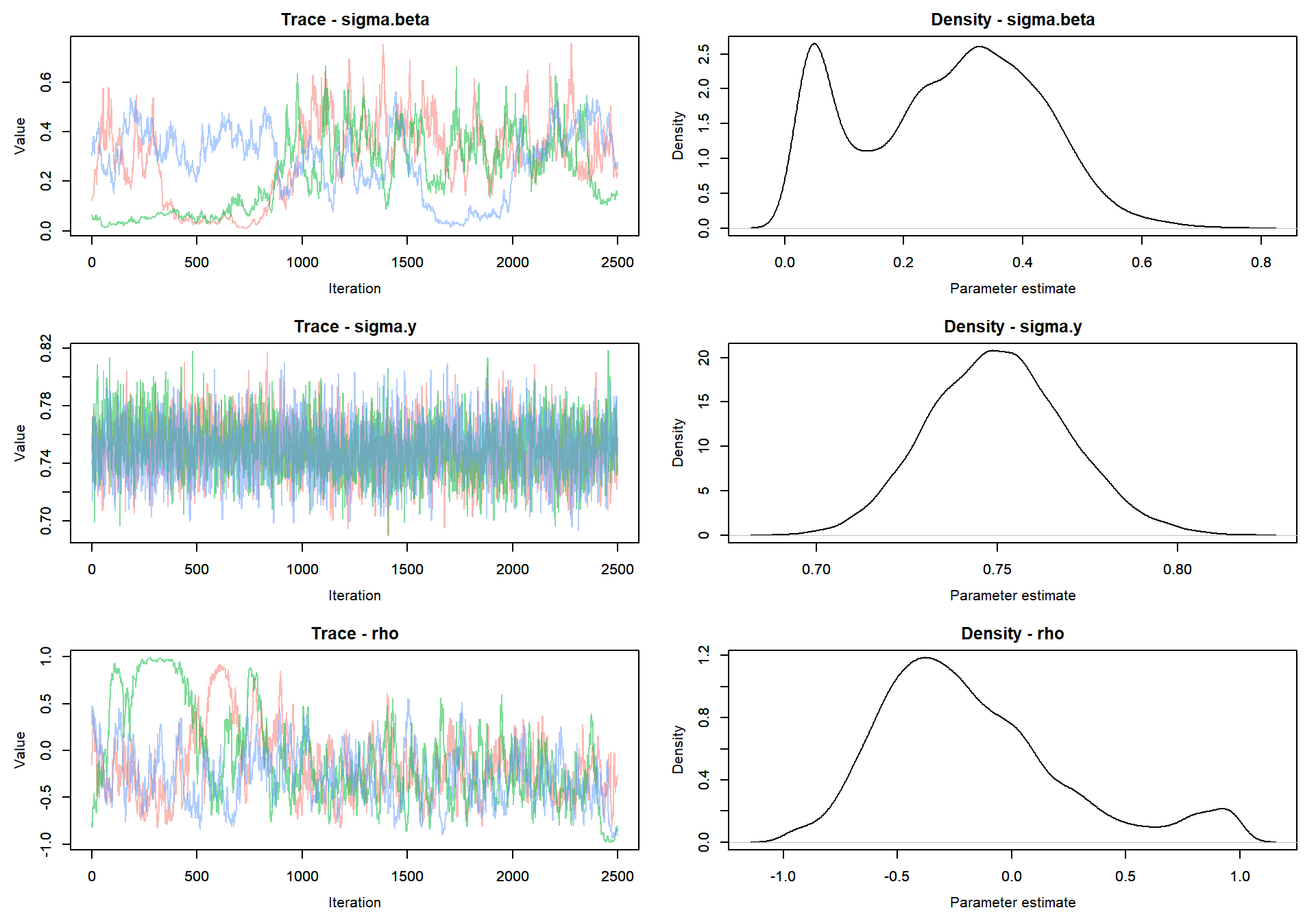
sigma.beta	0.2689	0.1517	0.0282	0.2854	0.5396	1.02	41
sigma.y	0.7504	0.0190	0.7147	0.7500	0.7888	1.00	1891
rho	-0.1768	0.4116	-0.7828	-0.2527	0.9074	1.06	140

Trace plot of parameters

MCMCvis::MCMCtrace(mlm_intslp_pred, params = params[!params %in% c("alpha", "beta")], pdf = FALSE )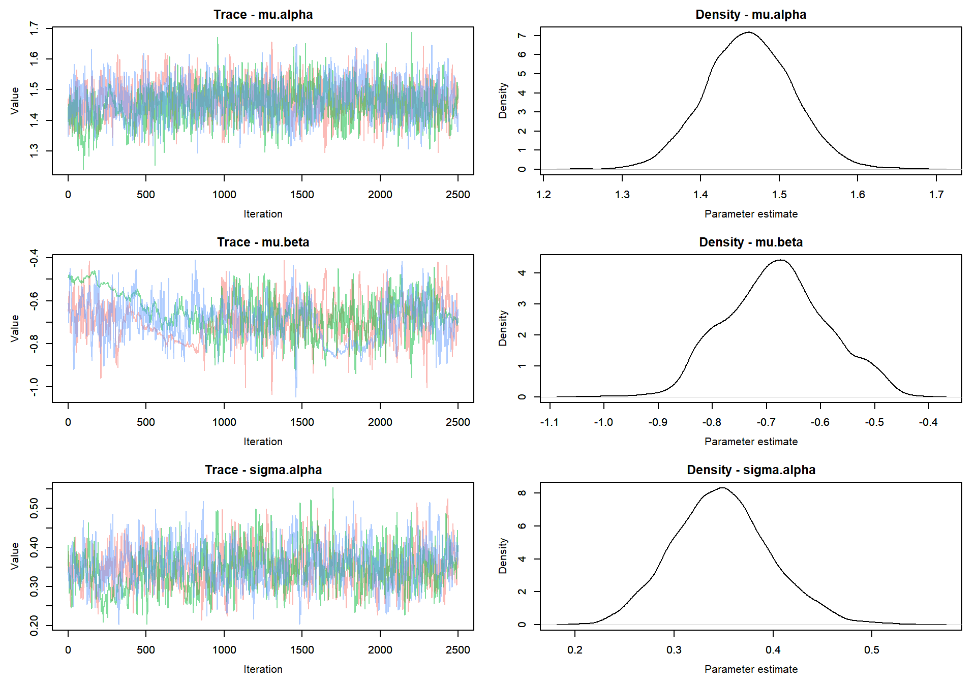

Compare fully Bayesian approach to linear mixed-effects model (via Restricted Maximum Likelihood [REML])

# compare
MCMCvis::MCMCsummary(mlm_intslp_pred, params = "alpha") %>% 
  data.frame() %>% 
  dplyr::select("mean") %>% 
  dplyr::slice_head(n = 8) %>% 
  dplyr::bind_cols(coef(M3)$county[1:8,"(Intercept)"]) %>% 
  dplyr::rename(Bayesian=1, LMM=2) %>% 
  kableExtra::kable(
    caption = "alpha predictions Bayesian vs. LMM (lme4::lmer)"
    , digits = 4
  ) %>% 
  kableExtra::kable_styling(font_size = 12)

Table 4.2: alpha predictions Bayesian vs. LMM (lme4::lmer)
	Bayesian	LMM
alpha[1]	1.1526	1.1445
alpha[2]	0.9326	0.9334
alpha[3]	1.4738	1.4717
alpha[4]	1.5203	1.5354
alpha[5]	1.4267	1.4270
alpha[6]	1.4805	1.4827
alpha[7]	1.8297	1.8194
alpha[8]	1.6816	1.6908

# compare
MCMCvis::MCMCsummary(mlm_intslp_pred, params = "beta") %>% 
  data.frame() %>% 
  dplyr::select("mean") %>% 
  dplyr::slice_head(n = 8) %>% 
  dplyr::bind_cols(coef(M3)$county[1:8,"x"]) %>% 
  dplyr::rename(Bayesian=1, LMM=2) %>% 
  kableExtra::kable(
    caption = "beta predictions Bayesian vs. LMM (lme4::lmer)"
    , digits = 4
  ) %>% 
  kableExtra::kable_styling(font_size = 12)

Table 4.2: beta predictions Bayesian vs. LMM (lme4::lmer)
	Bayesian	LMM
beta[1]	-0.5844	-0.5406
beta[2]	-0.7544	-0.7708
beta[3]	-0.6696	-0.6689
beta[4]	-0.7284	-0.7526
beta[5]	-0.6362	-0.6207
beta[6]	-0.6848	-0.6877
beta[7]	-0.5250	-0.4748
beta[8]	-0.6849	-0.6975

4.4 Including group-level predictors (p. 280)

We can expand the varying-intercept, varying-slope model including \(x\) of (\(\alpha\) and \(\beta\)) by including a group-level predictor (in this case, soil uranium):

4.4.1 Using `lme4::lmer` (p. 281)

## Including group level predictors
M4 <- lme4::lmer(data = radon_mn, formula = y ~ x + u + x:u + (1 + x | county))
summary(M4)

Linear mixed model fit by REML [‘lmerMod’] Formula: y ~ x + u + x:u + (1 + x | county) Data: radon_mn

REML criterion at convergence: 2132.2

Scaled residuals: Min 1Q Median 3Q Max -5.2770 -0.6057 0.0507 0.6288 3.4495

Random effects: Groups Name Variance Std.Dev. Corr county (Intercept) 0.0000 0.0000
x 0.1392 0.3731 NaN Residual 0.5735 0.7573
Number of obs: 919, groups: county, 85

Fixed effects: Estimate Std. Error t value (Intercept) 1.44407 0.02926 49.353 x -0.64131 0.08915 -7.194 u 0.84628 0.07476 11.320 x:u -0.41582 0.23894 -1.740

Correlation of Fixed Effects: (Intr) x u
x -0.328
u 0.354 -0.116
x:u -0.111 0.155 -0.313 optimizer (nloptwrap) convergence code: 0 (OK) boundary (singular) fit: see help(‘isSingular’)

#estimated regression coefficicents
coef(M4)$county[1:3,]

                 (Intercept)          x         u        x:u

AITKIN 1.444075 -0.5861689 0.8462757 -0.4158211 ANOKA 1.444075 -0.9559927 0.8462757 -0.4158211 BECKER 1.444075 -0.6121327 0.8462757 -0.4158211

# fixed and random effects
fixef(M4)

(Intercept) x u x:u 1.4440747 -0.6413080 0.8462757 -0.4158211

ranef(M4)$county[1:3,]

                 (Intercept)           x

AITKIN 0 0.05513916 ANOKA 0 -0.31468472 BECKER 0 0.02917531

# check intercept match for county 1
fixef(M4)["(Intercept)"] + fixef(M4)["u"] * u$u[1] + ranef(M4)$county[1,"(Intercept)"]

(Intercept) 0.8609504

coef(M4)$county[1,"(Intercept)"]

[1] 1.444075

# check slope match for county 1
fixef(M4)["x"] + fixef(M4)["x:u"] * u$u[1] + ranef(M4)$county[1,"x"]

-0.2996483

coef(M4)$county[1,"x"]

[1] -0.5861689

print("!!! yoinks! this doesn't align with book but the data and code are the same as the book...maybe bayes can help")

[1] “!!! yoinks! this doesn’t align with book but the data and code are the same as the book…maybe bayes can help”

yoinks! this doesn’t align with book but the data and code are the same as the book…maybe bayes can help

4.4.2 Bayesian

4.4.2.1 Data and Initial conditions

# varying-intercept model, no predictors
## data for jags
data <- list(
  n = nrow(radon_mn)
  , J = radon_mn$county %>% unique() %>% length()
  , y = radon_mn$log.radon %>% as.double()
  , x = radon_mn$x %>% as.double()
  , county = radon_mn$county_index %>% as.double()
  , u = u$u %>% as.double()
)
## inits for jags
inits <- function(){
  list(
    B.matrix = array(data = rnorm(n=2*data$J, mean = 0, sd = 1), dim = c(data$J,2)) # 2 = num. model params
    # mu.alpha
    , gamma.alpha0 = rnorm(1, mean = 0, sd = 1)
    , gamma.alpha1 = rnorm(1, mean = 0, sd = 1)
    # mu.beta
    , gamma.beta0 = rnorm(1, mean = 0, sd = 1)
    , gamma.beta1 = rnorm(1, mean = 0, sd = 1)
    , sigma.alpha = runif(n = 1, min = 0, max = 1)
    , sigma.beta = runif(n = 1, min = 0, max = 1)
    , sigma.y = runif(n = 1, min = 0, max = 1)
    , rho = runif(n = 1, min = -1, max = 1)
  )
}
# define parameters to return from MCMC
params <- c (
  "alpha"
  , "beta"
  # mu.alpha
  , "gamma.alpha0"
  , "gamma.alpha1"
  # mu.beta
  , "gamma.beta0"
  , "gamma.beta1"
  , "sigma.alpha"
  , "sigma.beta"
  , "sigma.y"
  , "rho"
)

4.4.2.2 JAGS Model

Recall model defined above

Write out the JAGS code for the model.

## JAGS Model
model {
  ###########################
  # priors
  ###########################
  # coefficient of correlation for covariance matrix
    rho ~ dunif(-1,1)
  # alpha priors
    sigma.alpha ~ dunif(0, 100)
    tau.alpha <- 1/sigma.alpha^2
    # mu.alpha
    gamma.alpha0 ~ dnorm(0, .0001)
    gamma.alpha1 ~ dnorm(0, .0001)
  # beta priors
    sigma.beta ~ dunif(0, 100)
    tau.beta <- 1/sigma.beta^2
    # mu.beta
    gamma.beta0 ~ dnorm(0, .0001)
    gamma.beta1 ~ dnorm(0, .0001)
  # y priors
    sigma.y ~ dunif(0, 100)
    tau.y <- 1/sigma.y^2
  ###########################
  # variance-covariance matrix
  ###########################
    # variance
    Sigma.matrix[1, 1] <- sigma.alpha^2 # row 1, column 1
    Sigma.matrix[2, 2] <- sigma.beta^2 # row 2, column 2
    # Cov(alpha,beta) = rho * sigma.alpha * sigma.beta
    Sigma.matrix[2, 1] <- rho * sigma.alpha * sigma.beta # row 2, column 1
    Sigma.matrix[1, 2] <- Sigma.matrix[2, 1] # row 1, column 2
    # invert Sigma matrix
    Omega.matrix <- inverse(Sigma.matrix)
  ###########################
  # likelihood
  ###########################
  # varying slopes and intercepts at the county level
    for(j in 1:J){
      mu.alpha[j] <- gamma.alpha0 + gamma.alpha1 * u[j]
      mu.beta[j] <- gamma.beta0 + gamma.beta1 * u[j]
      # put mu.alpha and mu.beta in matrix
      B.hat[j,1] <- mu.alpha[j] # column 1
      B.hat[j,2] <- mu.beta[j] # column 2
      # note multivariate normal
      B.matrix[j,1:2] ~ dmnorm(B.hat[j,], Omega.matrix)
      # extract alpha and beta from matrix
      alpha[j] <- B.matrix[j, 1] # column 1
      beta[j] <- B.matrix[j, 2] # column 2
    }
  # y
  for (i in 1:n){
    mu.y[i] <- alpha[county[i]] + beta[county[i]] * x[i]
    y[i] ~ dnorm(mu.y[i], tau.y)
  }
}

4.4.2.3 Implement JAGS Model

##################################################################
# insert JAGS model code into an R script
##################################################################
{ # Extra bracket needed only for R markdown files - see answers
  sink("intslp_grp_pred.R") # This is the file name for the jags code
  cat("
  ## JAGS Model
  model {
    ###########################
    # priors
    ###########################
    # coefficient of correlation for covariance matrix
      rho ~ dunif(-1,1)
    # alpha priors
      sigma.alpha ~ dunif(0, 100)
      tau.alpha <- 1/sigma.alpha^2
      # mu.alpha
      gamma.alpha0 ~ dnorm(0, .0001)
      gamma.alpha1 ~ dnorm(0, .0001)
    # beta priors
      sigma.beta ~ dunif(0, 100)
      tau.beta <- 1/sigma.beta^2
      # mu.beta
      gamma.beta0 ~ dnorm(0, .0001)
      gamma.beta1 ~ dnorm(0, .0001)
    # y priors
      sigma.y ~ dunif(0, 100)
      tau.y <- 1/sigma.y^2
    ###########################
    # variance-covariance matrix
    ###########################
      # variance
      Sigma.matrix[1, 1] <- sigma.alpha^2 # row 1, column 1
      Sigma.matrix[2, 2] <- sigma.beta^2 # row 2, column 2
      # Cov(alpha,beta) = rho * sigma.alpha * sigma.beta
      Sigma.matrix[2, 1] <- rho * sigma.alpha * sigma.beta # row 2, column 1
      Sigma.matrix[1, 2] <- Sigma.matrix[2, 1] # row 1, column 2
      # invert Sigma matrix
      Omega.matrix <- inverse(Sigma.matrix)
    ###########################
    # likelihood
    ###########################
    # varying slopes and intercepts at the county level
      for(j in 1:J){
        mu.alpha[j] <- gamma.alpha0 + gamma.alpha1 * u[j]
        mu.beta[j] <- gamma.beta0 + gamma.beta1 * u[j]
        # put mu.alpha and mu.beta in matrix
        B.hat[j,1] <- mu.alpha[j] # column 1
        B.hat[j,2] <- mu.beta[j] # column 2
        # note multivariate normal
        B.matrix[j,1:2] ~ dmnorm(B.hat[j,], Omega.matrix)
        # extract alpha and beta from matrix
        alpha[j] <- B.matrix[j, 1] # column 1
        beta[j] <- B.matrix[j, 2] # column 2
      }
    # y
    for (i in 1:n){
      mu.y[i] <- alpha[county[i]] + beta[county[i]] * x[i]
      y[i] ~ dnorm(mu.y[i], tau.y)
    }
  }
  ", fill = TRUE)
  sink()
}
##################################################################
# implement model
##################################################################
######################
# Call to JAGS
######################
intslp_grp_pred = rjags::jags.model(
  file = "intslp_grp_pred.R"
  , data = data
  , inits = inits
  , n.chains = 3
  , n.adapt = 1000
)

## Compiling model graph
##    Resolving undeclared variables
##    Allocating nodes
## Graph information:
##    Observed stochastic nodes: 919
##    Unobserved stochastic nodes: 93
##    Total graph size: 3837
## 
## Initializing model

stats::update(intslp_grp_pred, n.iter = 1000, progress.bar = "none")
# save the coda object (more precisely, an mcmc.list object) to R
mlm_intslp_grp_pred = rjags::coda.samples(
  model = intslp_grp_pred
  , variable.names = params
  , n.iter = 5000
  , n.thin = 1
  , progress.bar = "none"
)

4.4.2.4 Summary of the marginal posterior distributions of the parameters

Compare to results from scaled inverse-Wishart JAGS model results

# summary
MCMCvis::MCMCsummary(mlm_intslp_grp_pred, params = params[!params %in% c("alpha", "beta")]) %>% 
  kableExtra::kable(
    caption = "Bayesian: Varying-intercept & slope multilevel model, floor of measurement predictor + county-level (grp) uranium"
    , digits = 4
  ) %>% 
  kableExtra::kable_styling(font_size = 12)

Table 4.3: Bayesian: Varying-intercept & slope multilevel model, floor of measurement predictor + county-level (grp) uranium
	mean	sd	2.5%	50%	97.5%	Rhat	n.eff
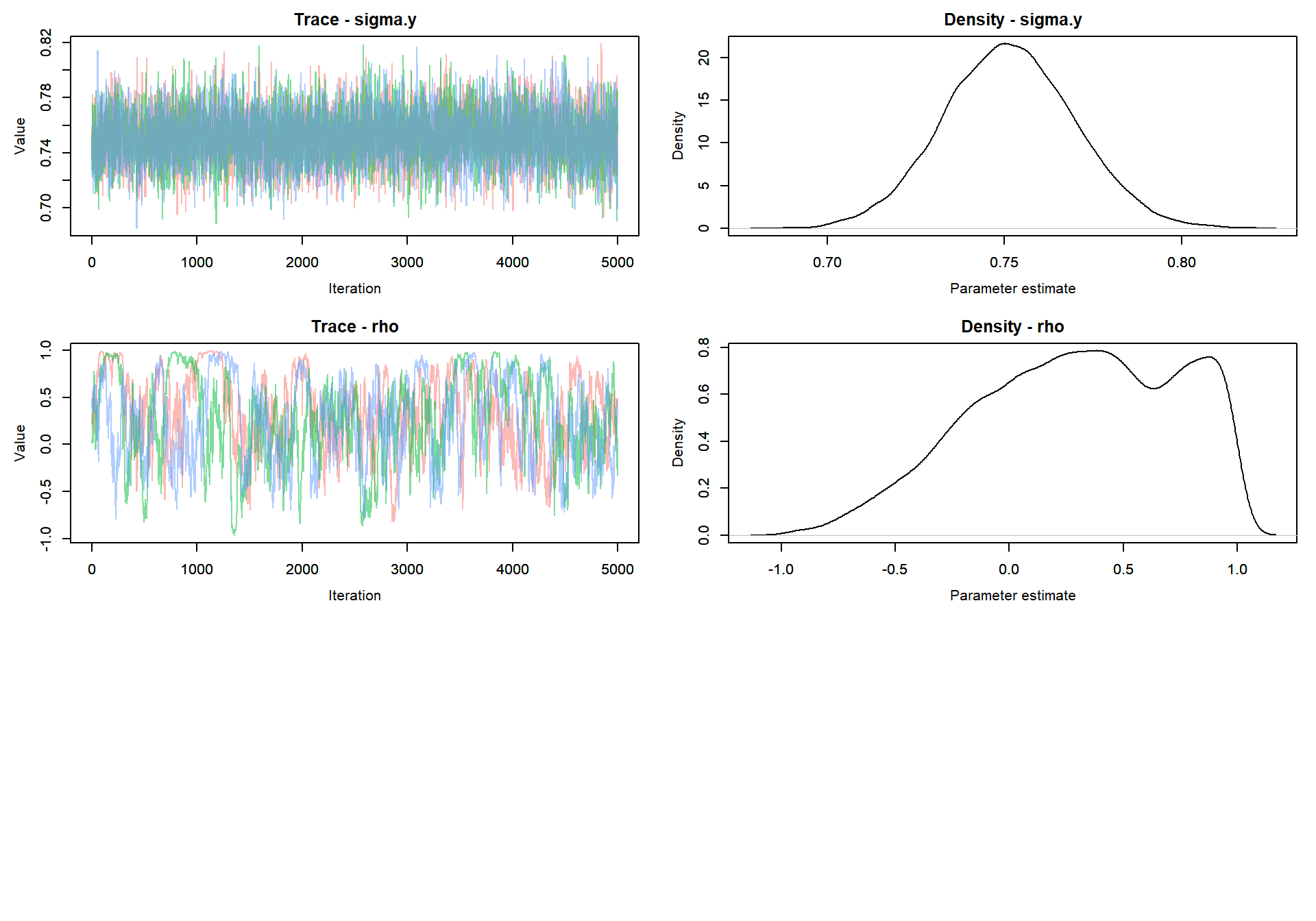
gamma.alpha0	1.4701	0.0363	1.3997	1.4702	1.5422	1.00	779
gamma.alpha1	0.8075	0.0941	0.6280	0.8071	0.9931	1.02	914
gamma.beta0	-0.6853	0.0888	-0.8510	-0.6886	-0.5007	1.00	569
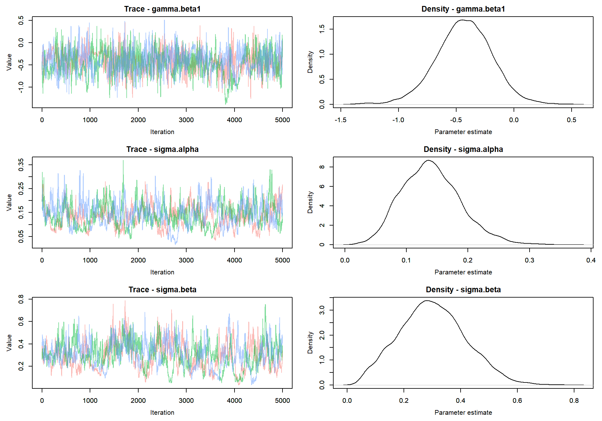
gamma.beta1	-0.4326	0.2414	-0.9258	-0.4300	0.0298	1.02	497
sigma.alpha	0.1401	0.0476	0.0571	0.1375	0.2444	1.01	233
sigma.beta	0.3009	0.1170	0.0850	0.2970	0.5389	1.01	188
sigma.y	0.7513	0.0185	0.7151	0.7511	0.7878	1.00	4958
rho	0.2917	0.4392	-0.5959	0.3146	0.9668	1.00	183

Trace plot of parameters

MCMCvis::MCMCtrace(mlm_intslp_grp_pred, params = params[!params %in% c("alpha", "beta")], pdf = FALSE )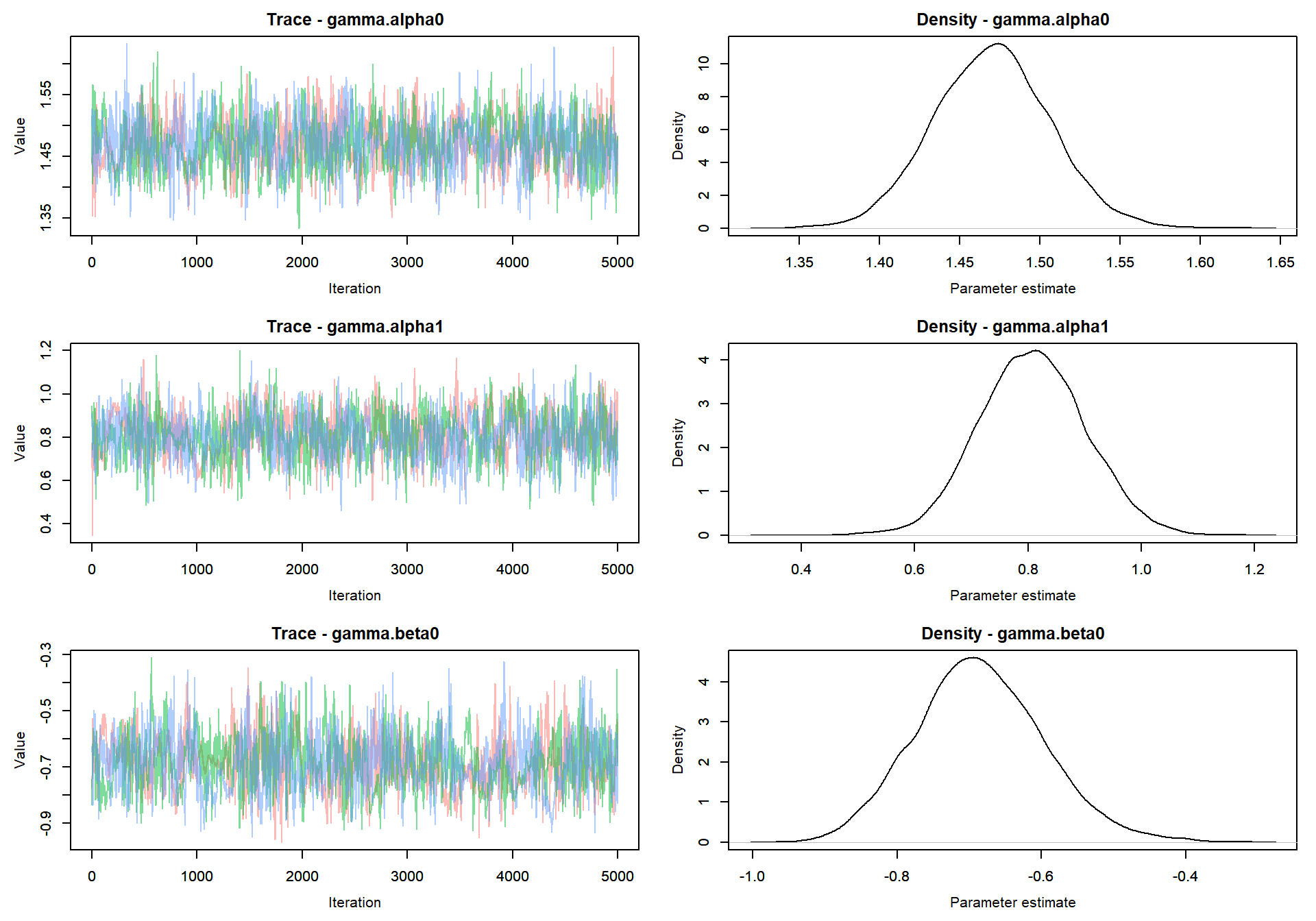

Caterpillar plot of parameters

# Caterpillar plots
MCMCvis::MCMCplot(mlm_intslp_grp_pred, params = params[!params %in% c("alpha", "beta")], xlim = c(-1,2))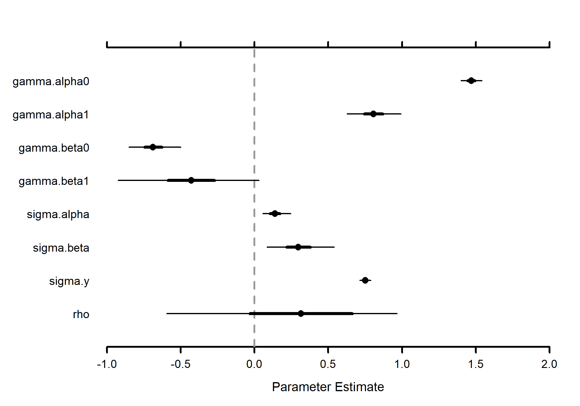

Compare fully Bayesian approach to linear mixed-effects model (via Restricted Maximum Likelihood [REML])

# compare
MCMCvis::MCMCsummary(mlm_intslp_grp_pred, params = "alpha") %>% 
  data.frame() %>% 
  dplyr::select("mean") %>% 
  dplyr::slice_head(n = 8) %>% 
  dplyr::bind_cols(coef(M4)$county[1:8,"(Intercept)"]) %>% 
  dplyr::rename(Bayesian=1, LMM=2) %>% 
  kableExtra::kable(
    caption = "alpha predictions Bayesian vs. LMM (lme4::lmer)"
    , digits = 4
  ) %>% 
  kableExtra::kable_styling(font_size = 12)

Table 4.4: alpha predictions Bayesian vs. LMM (lme4::lmer)
	Bayesian	LMM
alpha[1]	0.8954	1.4441
alpha[2]	0.8180	1.4441
alpha[3]	1.3888	1.4441
alpha[4]	1.0627	1.4441
alpha[5]	1.3640	1.4441
alpha[6]	1.7555	1.4441
alpha[7]	1.8028	1.4441
alpha[8]	1.7393	1.4441

# compare
MCMCvis::MCMCsummary(mlm_intslp_grp_pred, params = "beta") %>% 
  data.frame() %>% 
  dplyr::select("mean") %>% 
  dplyr::slice_head(n = 8) %>% 
  dplyr::bind_cols(coef(M4)$county[1:8,"x"]) %>% 
  dplyr::rename(Bayesian=1, LMM=2) %>% 
  kableExtra::kable(
    caption = "beta predictions Bayesian vs. LMM (lme4::lmer)"
    , digits = 4
  ) %>% 
  kableExtra::kable_styling(font_size = 12)

Table 4.4: beta predictions Bayesian vs. LMM (lme4::lmer)
	Bayesian	LMM
beta[1]	-0.3568	-0.5862
beta[2]	-0.5320	-0.9560
beta[3]	-0.6137	-0.6121
beta[4]	-0.3763	-0.5563
beta[5]	-0.5779	-0.5781
beta[6]	-0.8663	-0.6413
beta[7]	-0.4844	-0.2199
beta[8]	-0.7457	-0.5665

4.4.2.5 Estimated \(\alpha_{j}\) versus uranium measurment

Replicate Figure 13.2a for the multilevel model where the intercept and the slope vary by county (p.281)

dta_temp <- dplyr::bind_cols(
  u
  , MCMCvis::MCMCpstr(mlm_intslp_grp_pred, params = "alpha", func = function(x) quantile(x, c(0.25, 0.5, 0.75))) %>%
      data.frame() %>% 
      dplyr::rename_with(
        ~ tolower(gsub(".", "", .x, fixed = TRUE))
      )
  ) %>% 
  dplyr::arrange(county_index)
ggplot(dta_temp, mapping = aes(x = u)) +
  geom_abline(
    intercept = MCMCvis::MCMCpstr(mlm_intslp_grp_pred, params = "gamma.alpha0", func = median) %>% unlist()
    , slope = MCMCvis::MCMCpstr(mlm_intslp_grp_pred, params = "gamma.alpha1", func = median) %>% unlist()
    , linetype = "dashed"
    , lwd = 1
    , color = "gray40"
  ) +
  geom_linerange(
    mapping = aes(ymin = alpha25, ymax = alpha75)
  ) +
  geom_point(
    mapping = aes(y = alpha50)
  ) +
  # scale_y_continuous(limits = c(0,2.5)) +
  ylab(latex2exp::TeX("$\\hat{\\alpha}_{j}$")) + 
  xlab("log(u)") +
  labs(
    title = latex2exp::TeX("Median model intercept ($\\hat{\\alpha}_{j}$) prediction for each county (j) versus county-level uranium measurement")
  ) +
  theme_bw() + 
  theme(
    axis.text.x = element_blank()
    , axis.ticks.x = element_blank()
    , panel.grid = element_blank()
  )

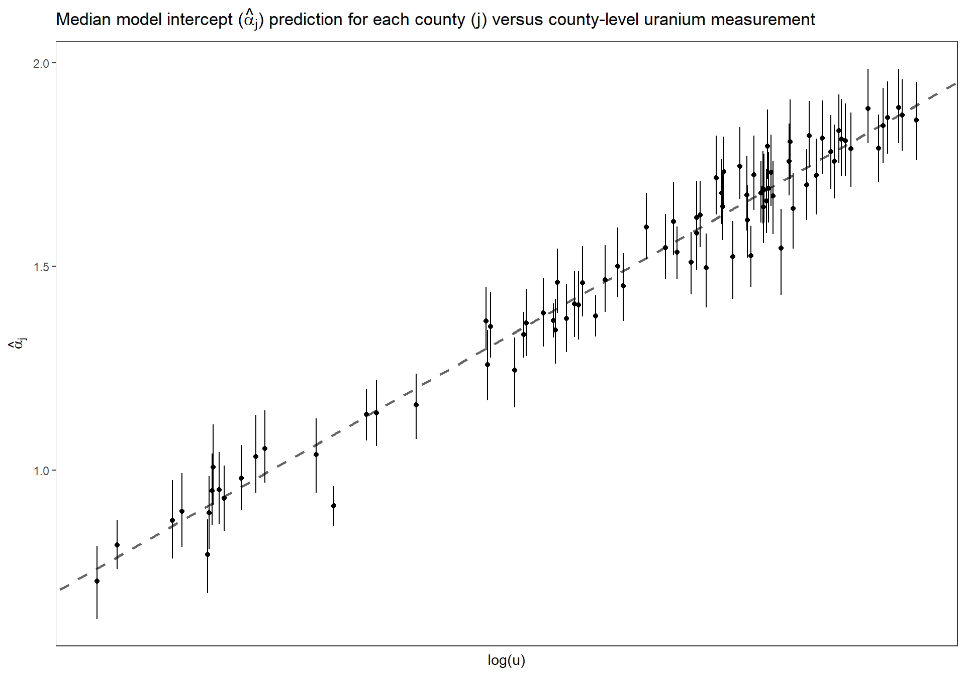
Estimated county coefficients \(\alpha_j\) plotted versus county-level uranium measurement \(u_j\), along with the estimated multilevel regression line \(\alpha_j = \gamma^{\alpha}_{0} + \gamma^{\alpha}_{1} \cdot u_j\). The county coefficients roughly follow the line but not exactly; the deviation of the coefficients from the line is captured in \(\sigma_{\alpha}\), the standard deviation of the errors in the county-level regression.

Replicate Figure 13.2b for the multilevel model where the intercept and the slope vary by county (p.281)

dta_temp <- dplyr::bind_cols(
  u
  , MCMCvis::MCMCpstr(mlm_intslp_grp_pred, params = "beta", func = function(x) quantile(x, c(0.25, 0.5, 0.75))) %>%
      data.frame() %>% 
      dplyr::rename_with(
        ~ tolower(gsub(".", "", .x, fixed = TRUE))
      )
  ) %>% 
  dplyr::arrange(county_index)
ggplot(dta_temp, mapping = aes(x = u)) +
  geom_abline(
    intercept = MCMCvis::MCMCpstr(mlm_intslp_grp_pred, params = "gamma.beta0", func = median) %>% unlist()
    , slope = MCMCvis::MCMCpstr(mlm_intslp_grp_pred, params = "gamma.beta1", func = median) %>% unlist()
    , linetype = "dashed"
    , lwd = 1
    , color = "gray40"
  ) +
  geom_linerange(
    mapping = aes(ymin = beta25, ymax = beta75)
  ) +
  geom_point(
    mapping = aes(y = beta50)
  ) +
  # scale_y_continuous(limits = c(0,2.5)) +
  ylab(latex2exp::TeX("$\\hat{\\beta}_{j}$")) + 
  xlab("log(u)") +
  labs(
    title = latex2exp::TeX("Median model slope ($\\hat{\\beta}_{j}$) prediction for each county (j) versus county-level uranium measurement")
  ) +
  theme_bw() + 
  theme(
    axis.text.x = element_blank()
    , axis.ticks.x = element_blank()
    , panel.grid = element_blank()
  )

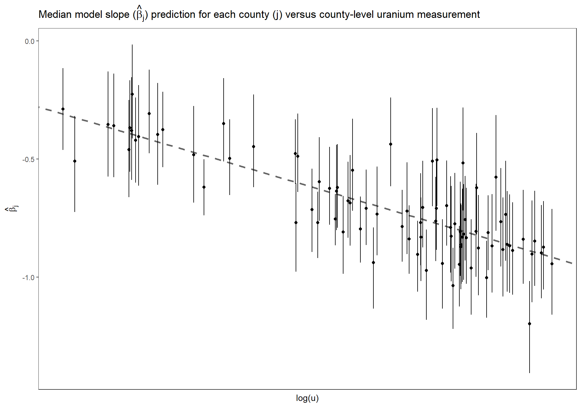
Estimated county coefficients \(\beta_j\) plotted versus county-level uranium measurement \(u_j\), along with the estimated multilevel regression line \(\beta_j = \gamma^{\beta}_{0} + \gamma^{\beta}_{1} \cdot u_j\). The county coefficients roughly follow the line but not exactly; the deviation of the coefficients from the line is captured in \(\sigma_{\beta}\), the standard deviation of the errors in the county-level regression.

4.5 Modeling multiple varying coefficients

When more than two coefficients vary (for example, \(y_i \sim \textrm{N}(\beta_{0} + \beta_{1} \cdot x_{i1} + \beta_{2} \cdot x_{i2}, \sigma^2_y)\) ), with \(\beta_0\), \(\beta_1\), and \(\beta_2\) varying by group), it is helpful to move to matrix notation (upper-case notation) in modeling the coefficients and their group-level regression model and covariance matrix (p.284)

More generally, we can have \(J\) groups, \(K\) individual-level predictors, and \(L\) predictors in the group-level regression (including the constant term as a predictor in both cases). For example, \(K = L = 2\) in the radon model that has floor as an individual predictor and uranium as a county-level predictor. To include group-level predictors (p.285):

\[\begin{align*} y_i &\sim \textrm{N}(X_{i} B_{j[i]}, \sigma^2_y) \\ &\textrm{for} \; i = 1, \cdots, n \\ B_j &\sim \textrm{N}(U_{j} G, \Sigma_B) \\ &\textrm{for} \; j = 1, \cdots, J \end{align*}\]

where

\(B\) is the \(J \times K\) matrix of individual-level coefficients,
\(U\) is the \(J \times L\) matrix of group-level predictors (including the constant term), and
\(G\) is the \(L \times K\) matrix of coefficients for the group-level regression.
\(U_j\) is the \(j^{th}\) row of \(U\), the vector of predictors for group \(j\), and so \(U_jG\) is a vector of length \(K\)
\(X\) is the \(n \times K\) matrix of predictors (e.g. \(x_{i1},x_{i2}, \cdots, x_{iK}\)), where \(K\) is the number of individual-level predictors (including the intercept) that vary by group. \(X_i\) is then the vector of length \(K\) representing the \(i^{th}\) row of \(X\)

When more than two coefficients are varying (for example, a varying intercept and two or more varying slopes), it is difficult to model the group-level correlations directly because of constraints involved in the requirement that the covariance matrix be positive definite. With more than two varying coefficients, it is simplest to just use the scaled inverse-Wishart model described above (p.286), using a full matrix notation to allow for an arbitrary number \(K\) of coefficients that vary by group (p.377)

4.5.1 JAGS Model (no group-level predictors; p.378)

Write out the JAGS code for the model.

A useful trick with the scaling is to define the coefficients \(\alpha_j\) , \(\beta_j\) in terms of multiplicative factors, \(\xi_\alpha\), \(\xi_\beta\), with unscaled parameters \(\alpha^{raw}_j\) , \(\beta^{raw}_j\) having the inverse-Wishart distribution.

model {
  ###########################
  # In R
  ###########################
    # J <- data$group_index %>% unique() %>% length()
    # X <- cbind(1,x)
    # K <- ncol(X)
    # W <- diag(K) # (KxK matrix with 1's on diagonal)
    # inits <- function(){
    #   list(
    #     B.raw = array(data = rnorm(n = J*K), dim = c(J,K))
    #     , mu.raw = rnorm(n = K)
    #     , sigma.y = runif(n = 1)
    #     , Tau.B.raw = rWishart(n = 1, df = K+1, Sigma = diag(K))
    #     , xi = runif(K)
    #   )
    # }
    # # parameters of interest
    # parameters <- c ("B", "mu", "sigma.y", "sigma.B", "rho.B")
  ###########################
  # priors
  ###########################
    ########
    # y priors
    ########
      sigma.y ~ dunif(0, 100)
      tau.y <- 1/sigma.y^2
    ########
    # define the coefficients for the intercept (e.g. alpha) and slope (e.g. beta)
      # in terms of multiplicative factors $\xi_\alpha$, $\xi_\beta$
      # with unscaled parameters $\alpha^{raw}_j$ , $\beta^{raw}_j$
    ########
      for(k in 1:K){
        xi[k] ~ dunif(0, 100)
        mu.raw[k] ~ dnorm(0, .0001)
        # parameter means (e.g. mu_alpha and mu_beta)
        mu[k] <- xi[k]*mu.raw[k]
      }
    ########
    # Specification of the Wishart distribution 
    ########
      # for the inverse-variance Tau.B.raw
      # , the matrix W is the prior scale
      # , which we set to the identity matrix (in R, we write W <- diag(K))
      # , and the degrees of freedom set to 1 more than the dimension of the matrix 
      #   (to induce a uniform prior distribution on rho)
      df <- K+1
      Tau.B.raw[1:K,1:K] ~ dwish(W[,], df)
      Sigma.B.raw[1:K,1:K] <- inverse(Tau.B.raw[,])
      # loop over K number of individual-level predictors 
        # (including the intercept) that vary by group
      for(k in 1:K){
        for(k.prime in 1:K){
          # coefficient of correlation (rho) for parameters
          rho.B[k,k.prime] <- Sigma.B.raw[k,k.prime] /
            sqrt(Sigma.B.raw[k,k]*Sigma.B.raw[k.prime,k.prime])
        }
        # variance for the intercept and slope parameters
        sigma.B[k] <- abs(xi[k])*sqrt(Sigma.B.raw[k,k])
      }
  ###########################
  # likelihood
  ###########################
  # varying slopes and intercepts
    for(j in 1:J){
      for(k in 1:K){
        # estimated slope and intercept coefficients
        B[j,k] <- xi[k]*B.raw[j,k]
      }
      B.raw[j,1:K] ~ dmnorm(mu.raw[], Tau.B.raw[,])
    }
  # y
    for(i in 1:n){
      # mu.y[i] <- alpha[county[i]] + beta[county[i]] * x[i]
      mu.y[i] <- inprod(B[county[i],],X[i,])
      y[i] ~ dnorm(mu.y[i], tau.y)
    }
}

4.5.2 JAGS Model (yes group-level predictors; p.379)

Multiple varying coefficients with multiple group-level predictors

Write out the JAGS code for the model.

This model is analogous to this model above but extends to models with multiple varying coefficients

model {
  ###########################
  # In R
  ###########################
    # J <- data$group_index %>% unique() %>% length()
    # X <- cbind(1,x) # x is of length i,...,n
    # K <- ncol(X)
    # W <- diag(K) # (KxK matrix with 1's on diagonal)
    # U <- cbind(1,u) # u is of length j,...,J
    # L <- ncol(U)
    # inits <- function(){
    #   list(
    #     B.raw = array(data = rnorm(n = J*K), dim = c(J,K))
    #     , G.raw = array(data = rnorm(n = L*K), dim = c(L,K))
    #     , sigma.y = runif(n = 1)
    #     , Tau.B.raw = rWishart(n = 1, df = K+1, Sigma = diag(K))
    #     , xi = runif(K)
    #   )
    # }
    # # parameters of interest
    # parameters <- c ("B", "G", "sigma.y", "sigma.B", "rho.B")
  ###########################
  # priors
  ###########################
    ########
    # y priors
    ########
      sigma.y ~ dunif(0, 100)
      tau.y <- 1/sigma.y^2
    ########
    # Modeling multiple group-level predictors
    ########
      # If we have several group-level predictors (expressed as a matrix U with J rows, one
      #   for each group), we use notation such as
      for (k in 1:K){
        for (l in 1:L){
          # parameter means (e.g. gamma.alpha0, gamma.alpha1, gamma.beta0, gamma.beta1)
          G[k,l] <- xi[k]*G.raw[k,l]
          G.raw[k,l] ~ dnorm(0, .0001)
        }
        xi[k] ~ dunif(0, 100)
      }
    ########
    # Specification of the Wishart distribution 
    ########
      # for the inverse-variance Tau.B.raw
      # , the matrix W is the prior scale
      # , which we set to the identity matrix (in R, we write W <- diag(K))
      # , and the degrees of freedom set to 1 more than the dimension of the matrix 
      #   (to induce a uniform prior distribution on rho)
      df <- K+1
      Tau.B.raw[1:K,1:K] ~ dwish(W[,], df)
      Sigma.B.raw[1:K,1:K] <- inverse(Tau.B.raw[,])
      # loop over K number of individual-level predictors 
        # (including the intercept) that vary by group
      for(k in 1:K){
        for(k.prime in 1:K){
          # coefficient of correlation (rho) for parameters
          rho.B[k,k.prime] <- Sigma.B.raw[k,k.prime] /
            sqrt(Sigma.B.raw[k,k]*Sigma.B.raw[k.prime,k.prime])
        }
        # variance for the intercept and slope parameters
        sigma.B[k] <- abs(xi[k])*sqrt(Sigma.B.raw[k,k])
      }
    ########
    # Modeling multiple varying coefficients
    ########
      # Modeling multiple varying coefficients
      for (j in 1:J){
        B.raw[j,1:K] ~ dmnorm(B.raw.hat[j,], Tau.B.raw[,])
        for (k in 1:K){
          # parameter means (e.g. mu.alpha[j] <- gamma.alpha0 + gamma.alpha1 * u[j])
          B.raw.hat[j,k] <- inprod(G.raw[k,],U[j,])
        }
      }
  ###########################
  # likelihood
  ###########################
  # varying slopes and intercepts
    for (k in 1:K){
      for (j in 1:J){
        # estimated slope and intercept coefficients
        B[j,k] <- xi[k]*B.raw[j,k]
      }
    }   

  # y
    for(i in 1:n){
      # mu.y[i] <- alpha[county[i]] + beta[county[i]] * x[i]
      mu.y[i] <- inprod(B[county[i],],X[i,])
      y[i] ~ dnorm(mu.y[i], tau.y)
    }
}

4.5.2.1 Data and Initial conditions

# select predictor variables for y model
x_vars_nms <- c("intercept", "x")
x_vars <- radon_mn %>% 
  dplyr::mutate(intercept = 1) %>% 
  dplyr::select(dplyr::any_of(x_vars_nms)) %>% 
  dplyr::mutate_if(is.numeric, as.double)
# select predictor variables for group-level model
grp_vars_nms <- c("intercept", "u")
grp_vars <- radon_mn %>% 
  dplyr::mutate(intercept = 1) %>% 
  dplyr::group_by(county_index) %>% 
  dplyr::summarise_at(grp_vars_nms, dplyr::first) %>% 
  dplyr::ungroup() %>% 
  dplyr::arrange(county_index) %>% 
  dplyr::select(dplyr::any_of(grp_vars_nms)) %>% 
  dplyr::mutate_if(is.numeric, as.double)
# set up matrix form
  J_temp <- radon_mn$county %>% unique() %>% length()
  # X_temp <- cbind(1, x_vars) # x_vars is of length i,...,n
  X_temp <- x_vars  # added intercept above in data definition
  K_temp <- ncol(X_temp)
  W_temp <- diag(K_temp) # (KxK matrix with 1's on diagonal)
  # U_temp <- cbind(1, grp_vars) # grp_vars is of length j,...,J
  U_temp <- grp_vars # added intercept above in data definition
  L_temp <- ncol(U_temp)
## data for jags
data <- list(
  n = nrow(radon_mn)
  , y = radon_mn$log.radon %>% as.double()
  , county = radon_mn$county_index %>% as.double()
  # matrix form
  , J = J_temp
  , X = X_temp
  , K = K_temp
  , W = W_temp
  , U = U_temp
  , L = L_temp
)
## inits for jags
inits <- function(){
  list(
    B.raw = array(data = rnorm(n = data$J*data$K, mean = 0, sd = 1), dim = c(data$J, data$K))
    , G.raw = array(data = rnorm(n = data$L*data$K), dim = c(data$L, data$K))
    , sigma.y = runif(n = 1, min = 0, max = 1)
    # , Tau.B.raw = rWishart(n = 1, df = data$K+1, Sigma = diag(data$K))
    , Tau.B.raw = monomvn::rwish(v = data$K+1, S = diag(data$K))
    , xi = runif(n = data$K, min = 0, max = 1)
  )
}
# define parameters to return from MCMC
params <- c (
  "B"
  , "G"
  , "sigma.y"
  , "sigma.B"
  , "rho.B"
)

4.5.2.2 Implement JAGS Model

##################################################################
# insert JAGS model code into an R script
##################################################################
{ # Extra bracket needed only for R markdown files - see answers
  sink("intslp_grp_pred_mtrx.R") # This is the file name for the jags code
  cat("
  model {
    ###########################
    # priors
    ###########################
      ########
      # y priors
      ########
        sigma.y ~ dunif(0, 100)
        tau.y <- 1/sigma.y^2
      ########
      # Modeling multiple group-level predictors
      ########
        # If we have several group-level predictors (expressed as a matrix U with J rows, one
        #   for each group), we use notation such as
        for (k in 1:K){
          for (l in 1:L){
            # parameter means (e.g. gamma.alpha0, gamma.alpha1, gamma.beta0, gamma.beta1)
            G[k,l] <- xi[k]*G.raw[k,l]
            G.raw[k,l] ~ dnorm(0, .0001)
          }
          xi[k] ~ dunif(0, 100)
        }
      ########
      # Specification of the Wishart distribution 
      ########
        # for the inverse-variance Tau.B.raw
        # , the matrix W is the prior scale
        # , which we set to the identity matrix (in R, we write W <- diag(K))
        # , and the degrees of freedom set to 1 more than the dimension of the matrix 
        #   (to induce a uniform prior distribution on rho)
        df <- K+1
        Tau.B.raw[1:K,1:K] ~ dwish(W[,], df)
        Sigma.B.raw[1:K,1:K] <- inverse(Tau.B.raw[,])
        # loop over K number of individual-level predictors 
          # (including the intercept) that vary by group
        for(k in 1:K){
          for(k.prime in 1:K){
            # coefficient of correlation (rho) for parameters
            rho.B[k,k.prime] <- Sigma.B.raw[k,k.prime] /
              sqrt(Sigma.B.raw[k,k]*Sigma.B.raw[k.prime,k.prime])
          }
          # variance for the intercept and slope parameters
          sigma.B[k] <- abs(xi[k])*sqrt(Sigma.B.raw[k,k])
        }
      ########
      # Modeling multiple varying coefficients
      ########
        # Modeling multiple varying coefficients
        for (j in 1:J){
          B.raw[j,1:K] ~ dmnorm(B.raw.hat[j,], Tau.B.raw[,])
          for (k in 1:K){
            # parameter means (e.g. mu.alpha[j] <- gamma.alpha0 + gamma.alpha1 * u[j])
            B.raw.hat[j,k] <- inprod(G.raw[k,],U[j,])
          }
        }
    ###########################
    # likelihood
    ###########################
    # varying slopes and intercepts
      for (k in 1:K){
        for (j in 1:J){
          # estimated slope and intercept coefficients
          B[j,k] <- xi[k]*B.raw[j,k]
        }
      }   
  
    # y
      for(i in 1:n){
        # mu.y[i] <- alpha[county[i]] + beta[county[i]] * x[i]
        mu.y[i] <- inprod(B[county[i],],X[i,])
        y[i] ~ dnorm(mu.y[i], tau.y)
      }
  }
  ", fill = TRUE)
  sink()
}
##################################################################
# implement model
##################################################################
######################
# Call to JAGS
######################
intslp_grp_pred_mtrx = rjags::jags.model(
  file = "intslp_grp_pred_mtrx.R"
  , data = data
  , inits = inits
  , n.chains = 3
  , n.adapt = 1000
)

## Compiling model graph
##    Resolving undeclared variables
##    Allocating nodes
## Graph information:
##    Observed stochastic nodes: 919
##    Unobserved stochastic nodes: 93
##    Total graph size: 5814
## 
## Initializing model

stats::update(intslp_grp_pred_mtrx, n.iter = 1000, progress.bar = "none")
# save the coda object (more precisely, an mcmc.list object) to R
mlm_intslp_grp_pred_mtrx = rjags::coda.samples(
  model = intslp_grp_pred_mtrx
  , variable.names = params
  , n.iter = 5000
  , n.thin = 1
  , progress.bar = "none"
)

4.5.2.3 Summary of the marginal posterior distributions of the parameters

Compare to results from multivariate normal JAGS model results where \(K = L = 2\)

# summary
MCMCvis::MCMCsummary(mlm_intslp_grp_pred_mtrx, params = params[!params %in% c("B")]) %>% 
  kableExtra::kable(
    caption = "Raw Results: Varying-intercept & slope multilevel model, floor of measurement predictor + county-level (grp) uranium"
    , digits = 4
  ) %>% 
  kableExtra::kable_styling(font_size = 12)

Table 4.5: Raw Results: Varying-intercept & slope multilevel model, floor of measurement predictor + county-level (grp) uranium
	mean	sd	2.5%	50%	97.5%	Rhat	n.eff
G[1,1]	1.4701	0.0389	1.3948	1.4698	1.5471	1.00	5757
G[2,1]	-0.6887	0.0776	-0.8410	-0.6888	-0.5351	1.00	3311
G[1,2]	0.7964	0.0972	0.6048	0.7984	0.9829	1.01	1380
G[2,2]	-0.4091	0.2066	-0.8199	-0.4053	-0.0343	1.04	277
sigma.y	0.7542	0.0187	0.7191	0.7538	0.7920	1.00	5328
sigma.B[1]	0.1588	0.0422	0.0852	0.1552	0.2508	1.01	442
sigma.B[2]	0.1616	0.1062	0.0244	0.1366	0.4130	1.12	127
rho.B[1,1]	1.0000	0.0000	1.0000	1.0000	1.0000	NaN	0
rho.B[2,1]	0.2304	0.3919	-0.5795	0.2726	0.8420	1.01	386
rho.B[1,2]	0.2304	0.3919	-0.5795	0.2726	0.8420	1.01	386
rho.B[2,2]	1.0000	0.0000	1.0000	1.0000	1.0000	NaN	0

Now clean results from matrix format

# function to name rows of G matrix
fn_g_mtrx_nm <- function(x_vars_nms, grp_vars_nms) {
  tidyr::expand_grid(grp_vars_nms, x_vars_nms) %>% 
  mutate(
    parameter = paste0("beta.", x_vars_nms, "_gamma.", grp_vars_nms)
  ) %>% 
  dplyr::select(parameter) %>% 
  c()
}
# function to name rows of sigma.B matrix
fn_sigmaB_mtrx_nm <- function(x_vars_nms) {
  paste0("sigma.", x_vars_nms)
}

# nice table of results
dplyr::bind_rows(
# gamma matrix
MCMCvis::MCMCsummary(mlm_intslp_grp_pred_mtrx, params = params[params %in% c("G")]) %>% 
  as.data.frame() %>% 
  cbind(parameter = fn_g_mtrx_nm(x_vars_nms, grp_vars_nms)) %>% 
  dplyr::relocate(parameter) %>% 
  dplyr::arrange(parameter)
# sigma.B matrix
, MCMCvis::MCMCsummary(mlm_intslp_grp_pred_mtrx, params = params[params %in% c("sigma.B")]) %>% 
  as.data.frame() %>% 
  cbind(parameter = fn_sigmaB_mtrx_nm(x_vars_nms)) %>% 
  dplyr::relocate(parameter)
# sigma.y
, MCMCvis::MCMCsummary(mlm_intslp_grp_pred_mtrx, params = params[params %in% c("sigma.y", "rho.B")]) %>% 
  as.data.frame() %>% 
  tibble::rownames_to_column(var = "parameter")
) %>%   
  kableExtra::kable(
    caption = "Cleaned Results: Varying-intercept & slope multilevel model, floor of measurement predictor + county-level (grp) uranium"
    , digits = 4
    , row.names = FALSE
  ) %>% 
  kableExtra::kable_styling(font_size = 12)

Table 4.6: Cleaned Results: Varying-intercept & slope multilevel model, floor of measurement predictor + county-level (grp) uranium
parameter	mean	sd	2.5%	50%	97.5%	Rhat	n.eff
beta.intercept_gamma.intercept	1.4701	0.0389	1.3948	1.4698	1.5471	1.00	5757
beta.intercept_gamma.u	0.7964	0.0972	0.6048	0.7984	0.9829	1.01	1380
beta.x_gamma.intercept	-0.6887	0.0776	-0.8410	-0.6888	-0.5351	1.00	3311
beta.x_gamma.u	-0.4091	0.2066	-0.8199	-0.4053	-0.0343	1.04	277
sigma.intercept	0.1588	0.0422	0.0852	0.1552	0.2508	1.01	442
sigma.x	0.1616	0.1062	0.0244	0.1366	0.4130	1.12	127
sigma.y	0.7542	0.0187	0.7191	0.7538	0.7920	1.00	5328
rho.B[1,1]	1.0000	0.0000	1.0000	1.0000	1.0000	NaN	0
rho.B[2,1]	0.2304	0.3919	-0.5795	0.2726	0.8420	1.01	386
rho.B[1,2]	0.2304	0.3919	-0.5795	0.2726	0.8420	1.01	386
rho.B[2,2]	1.0000	0.0000	1.0000	1.0000	1.0000	NaN	0

4.6 Non-nested models (p.289)

4.6.1 Example 1:

a psychological experiment with two potentially interacting factors

Data is from a psychological experiment of pilots on flight simulators, with \(n = 40\) data points corresponding to \(J = 5\) treatment conditions and \(K = 8\) different airports (e.g. sites, species, etc.). The responses can be fit to a non-nested multilevel model of the form:

\[\begin{align*} y_i &\sim \textrm{N}(\mu + \gamma_{j[i]} + \delta_{k[i]}, \sigma^2_y) \\ &\textrm{for} \; i = 1, \cdots, n \\ \gamma_j &\sim \textrm{N}(0, \sigma^2_{\gamma}) \\ &\textrm{for} \; j = 1, \cdots, J \\ \delta_k &\sim \textrm{N}(0, \sigma^2_{\delta}) \\ &\textrm{for} \; k = 1, \cdots, K \end{align*}\]

The parameters \(\gamma_j\) and \(\delta_k\) represent treatment effects and airport effects. Their distributions are centered at zero (rather than given mean levels \(\mu_\gamma\) and \(\mu_\delta\)) because the regression model for \(y\) already has an intercept, \(\mu\), and any nonzero mean for the \(\gamma\) and \(\delta\) distributions could be folded into \(\mu\). As we shall see in Section 19.4, it can sometimes be effective for computational purposes to add extra mean-level parameters into the model, but the coefficients in this expanded model must be interpreted with care. We can perform a quick fit as follows:

4.6.1.1 Load Data

# pilots <- read.table("http://www.stat.columbia.edu/~gelman/arm/examples/pilots/pilots.dat", header=TRUE, sep=",") %>% 
pilots <- read.table("../data/pilots/pilots.dat", header=TRUE) %>% 
  dplyr::filter(recovered %in% c(0,1)) %>% 
  dplyr::group_by(group, scenario) %>% 
  dplyr::summarize(
    successes = sum(recovered, na.rm = TRUE)
    , trials = n()
  ) %>% 
  dplyr::ungroup() %>% 
  dplyr::mutate(
    y = successes / trials
    , treatment_index = as.numeric(as.factor(group)) 
    , site_index = as.numeric(as.factor(scenario))
  )
# scenario.abbr <- c("Nagoya", "B'ham", "Detroit", "Ptsbgh", "Roseln", "Chrlt", "Shemya", "Toledo")

4.6.1.2 Using `lme4::lmer` (p. 289)

## Model fit
M1 <- lme4::lmer(data = pilots, formula = y ~ 1 + (1 | treatment_index) + (1 | site_index))
summary(M1)

## Linear mixed model fit by REML ['lmerMod']
## Formula: y ~ 1 + (1 | treatment_index) + (1 | site_index)
##    Data: pilots
## 
## REML criterion at convergence: 12.3
## 
## Scaled residuals: 
##      Min       1Q   Median       3Q      Max 
## -1.30647 -0.66461 -0.07957  0.33792  2.96201 
## 
## Random effects:
##  Groups          Name        Variance Std.Dev.
##  site_index      (Intercept) 0.10333  0.3214  
##  treatment_index (Intercept) 0.00000  0.0000  
##  Residual                    0.04674  0.2162  
## Number of obs: 40, groups:  site_index, 8; treatment_index, 5
## 
## Fixed effects:
##             Estimate Std. Error t value
## (Intercept)   0.4418     0.1187   3.723
## optimizer (nloptwrap) convergence code: 0 (OK)
## boundary (singular) fit: see help('isSingular')

4.6.1.3 Bayesian

4.6.1.3.1 Data and Initial conditions

## data for jags
data <- list(
  n = nrow(pilots)
  , J = pilots$treatment_index %>% unique() %>% length()
  , K = pilots$site_index %>% unique() %>% length()
  , y = pilots$y %>% as.double()
  , treatment = pilots$treatment_index %>% as.double()
  , site = pilots$site_index %>% as.double()
)
## inits for jags
inits <- function(){
  list(
    mu = rnorm(1, mean = 0, sd = 1)
    , gamma = rnorm(n = data$J, mean = 0, sd = 1) # treatment effects (j)
    , delta = rnorm(n = data$K, mean = 0, sd = 1) # site effects (k)
    , sigma.gamma = runif(n = 1, min = 0, max = 1)
    , sigma.delta = runif(n = 1, min = 0, max = 1)
    , sigma.y = runif(n = 1, min = 0, max = 1)
  )
}
# define parameters to return from MCMC
params <- c (
  "mu"
  , "gamma"
  , "delta"
  , "sigma.gamma"
  , "sigma.delta"
  , "sigma.y"
)

4.6.1.4 JAGS Model

Recall model defined above

Write out the JAGS code for the model.

## JAGS Model
model {
  ###########################
  # priors
  ###########################
  # mu priors
    mu ~ dnorm(0,1E-6)
  # gamma priors
    sigma.gamma ~ dunif(0, 100)
    tau.gamma <- 1/sigma.gamma^2
    mu.gamma <- 0
  # delta priors
    sigma.delta ~ dunif(0, 100)
    tau.delta <- 1/sigma.delta^2
    mu.delta <- 0
  # y priors
    sigma.y ~ dunif(0, 100)
    tau.y <- 1/sigma.y^2
  ###########################
  # likelihood
  ###########################
  # treatment effects (j)
    for (j in 1:J){
      gamma[j] ~ dnorm(mu.gamma, tau.gamma)
    }
  # site effects (k)
    for (k in 1:K){
      delta[k] ~ dnorm(mu.delta, tau.delta)
    }
  # y
  for (i in 1:n){
    mu.y[i] <- mu + gamma[treatment[i]] + delta[site[i]]
    y[i] ~ dnorm(mu.y[i], tau.y)
  }
}

4.6.1.5 Implement JAGS Model

##################################################################
# insert JAGS model code into an R script
##################################################################
{ # Extra bracket needed only for R markdown files - see answers
  sink("pilots_pred1.R") # This is the file name for the jags code
  cat("
  ## JAGS Model
  model {
    ###########################
    # priors
    ###########################
    # mu priors
      mu ~ dnorm(0,1E-6)
    # gamma priors
      sigma.gamma ~ dunif(0, 100)
      tau.gamma <- 1/sigma.gamma^2
      mu.gamma <- 0
    # delta priors
      sigma.delta ~ dunif(0, 100)
      tau.delta <- 1/sigma.delta^2
      mu.delta <- 0
    # y priors
      sigma.y ~ dunif(0, 100)
      tau.y <- 1/sigma.y^2
    ###########################
    # likelihood
    ###########################
    # treatment effects (j)
      for (j in 1:J){
        gamma[j] ~ dnorm(mu.gamma, tau.gamma)
      }
    # site effects (k)
      for (k in 1:K){
        delta[k] ~ dnorm(mu.delta, tau.delta)
      }
    # y
    for (i in 1:n){
      mu.y[i] <- mu + gamma[treatment[i]] + delta[site[i]]
      y[i] ~ dnorm(mu.y[i], tau.y)
    }
  }
  ", fill = TRUE)
  sink()
}
##################################################################
# implement model
##################################################################
######################
# Call to JAGS
######################
pilots_pred1 = rjags::jags.model(
  file = "pilots_pred1.R"
  , data = data
  , inits = inits
  , n.chains = 3
  , n.adapt = 100
)

## Compiling model graph
##    Resolving undeclared variables
##    Allocating nodes
## Graph information:
##    Observed stochastic nodes: 40
##    Unobserved stochastic nodes: 17
##    Total graph size: 191
## 
## Initializing model

stats::update(pilots_pred1, n.iter = 1000, progress.bar = "none")
# save the coda object (more precisely, an mcmc.list object) to R
mlm_pilots_pred1 = rjags::coda.samples(
  model = pilots_pred1
  , variable.names = params
  , n.iter = 1000
  , n.thin = 1
  , progress.bar = "none"
)

4.6.1.6 Summary of the marginal posterior distributions of the parameters

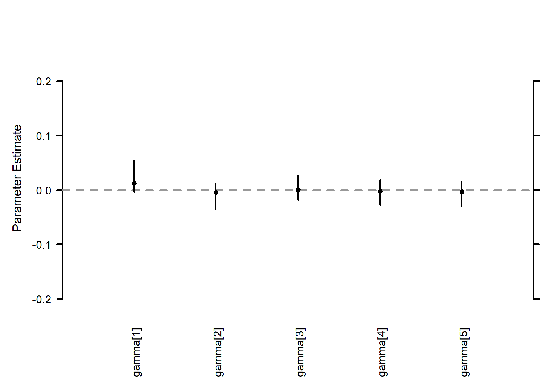
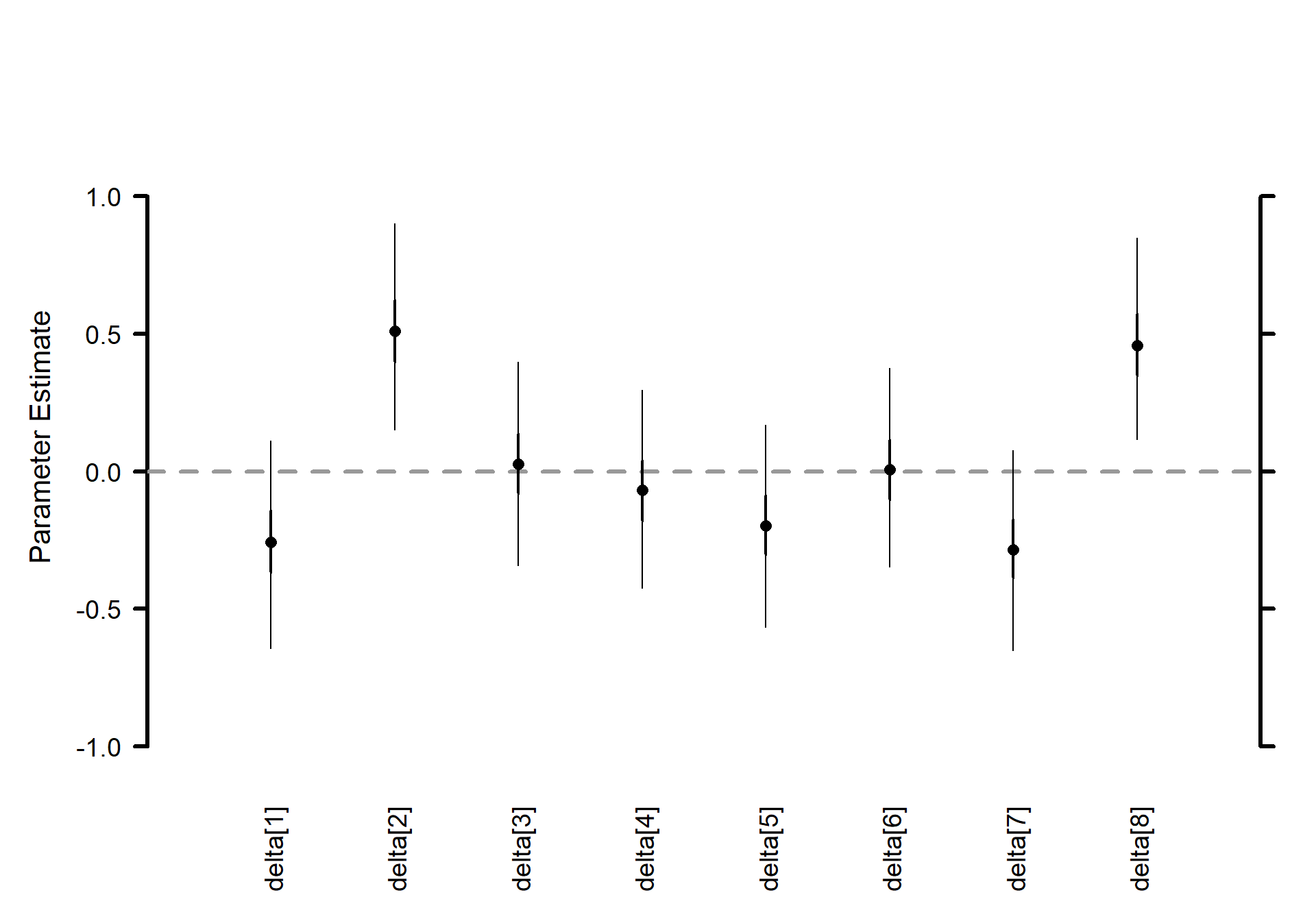
Thus, the variation among sites (airports) is huge \(\sigma_\delta\) – even larger than that among individual measurements \(\sigma_y\) – but the treatments \(\sigma_\gamma\) vary almost not at all.

# summary
MCMCvis::MCMCsummary(mlm_pilots_pred1, params = params[!params %in% c("gamma", "delta")]) %>% 
  kableExtra::kable(
    caption = "Bayesian: treatment and site effects model"
    , digits = 4
  ) %>% 
  kableExtra::kable_styling(font_size = 12)

Table 4.7: Bayesian: treatment and site effects model
	mean	sd	2.5%	50%	97.5%	Rhat	n.eff
mu	0.4126	0.1648	0.0851	0.4179	0.7381	1.05	90
sigma.gamma	0.0618	0.0518	0.0029	0.0483	0.1982	1.03	200
sigma.delta	0.4052	0.1726	0.2090	0.3693	0.8122	1.06	375
sigma.y	0.2270	0.0294	0.1776	0.2250	0.2911	1.00	1230

Treatment effects \(\boldsymbol{\gamma}\) (J=5) horizontal caterpillar plot

# Caterpillar plots
MCMCvis::MCMCplot(
  mlm_pilots_pred1
  , params = c("gamma")
  , horiz = FALSE
  , sz_med = 1.2, sz_thick = 2, sz_thin = 1
)

Site (airport) effects \(\boldsymbol{\delta}\) (K=8) horizontal caterpillar plot

# Caterpillar plots
MCMCvis::MCMCplot(
  mlm_pilots_pred1
  , params = c("delta")
  , horiz = FALSE
  , sz_med = 1.2, sz_thick = 2, sz_thin = 1
)

4.6.2 Example 2:

regression of earnings on ethnicity categories, age categories, and height

All the ideas of the earlier part of this chapter, introduced in the context of a simple structure of individuals within groups, apply to non-nested models as well. Here, we estimate a regression of log earnings, \(y_i\), on height, \(z_i\) (mean-adjusted), applied to the J = 4 ethnic groups (e.g. treatments) and K = 3 age categories (e.g. species). In essence, there is a separate regression model for each age group and ethnicity combination. The multilevel model can be written, somewhat awkwardly, as a data-level model,

\[ \begin{align*} y_i &\sim \textrm{N}(\alpha_{j[i],k[i]} + \beta_{j[i],k[i]} \cdot z_i , \sigma^2_y) \\ &\textrm{for} \; i = 1, \cdots, n \end{align*} \] a decomposition of the intercepts and slopes into terms for ethnicity, age, and ethnicity \(\times\) age,

\[ \begin{align*} \left(\begin{array}{c} \alpha_{j,k}\\ \beta_{j,k} \end{array}\right) &= \left(\begin{array}{c} \mu_{0}\\ \mu_{1} \end{array}\right) + \left(\begin{array}{c} \gamma_{0j}^\textrm{eth}\\ \gamma_{1j}^\textrm{eth} \end{array}\right) + \left(\begin{array}{c} \gamma_{0k}^\textrm{age}\\ \gamma_{1k}^\textrm{age} \end{array}\right) + \left(\begin{array}{c} \gamma_{0jk}^{\textrm{eth} \times \textrm{age}}\\ \gamma_{1jk}^{\textrm{eth} \times \textrm{age}} \end{array}\right) \end{align*} \]

and models for variation,

\[ \begin{align*} \left(\begin{array}{c} \gamma_{0j}^\textrm{eth}\\ \gamma_{1j}^\textrm{eth} \end{array}\right) &\sim \textrm{N}\left(\left(\begin{array}{c} 0\\ 0 \end{array}\right) , \Sigma^{\textrm{eth}} \right) \\ &\textrm{for} \; j = 1, \cdots, J \\ \left(\begin{array}{c} \gamma_{0k}^\textrm{age}\\ \gamma_{1k}^\textrm{age} \end{array}\right) &\sim \textrm{N}\left(\left(\begin{array}{c} 0\\ 0 \end{array}\right) , \Sigma^{\textrm{age}} \right) \\ &\textrm{for} \; k = 1, \cdots, K \\ \left(\begin{array}{c} \gamma_{0jk}^{\textrm{eth} \times \textrm{age}}\\ \gamma_{1jk}^{\textrm{eth} \times \textrm{age}} \end{array}\right) &\sim \textrm{N}\left(\left(\begin{array}{c} 0\\ 0 \end{array}\right) , \Sigma^{\textrm{eth} \times \textrm{age}} \right) \\ &\textrm{for} \; j = 1, \cdots, J \, \textrm{;} \, k = 1, \cdots, K \end{align*} \]

Because we have included means \(\mu_0\), \(\mu_1\) in the decomposition above, we can center each batch of coefficients at 0.

We fit this model, and the subsequent models in this chapter, in Bugs (see Chapter 17 for examples of code) because lme4::lmer() does not work so well when the number of groups is small—and, conversely, with these small datasets, Bugs is not too slow.

Chapter 4 Multilevel linear models: varying slopes, non-nested models, and other complexities (Ch 13)

4.1 Setup

4.2 Load data

4.3 Varying intercepts and slopes (p. 279)

4.3.1 Using lme4::lmer (p. 279)

4.3.2 Bayesian

4.3.2.1 Data and Initial conditions

4.3.2.2 JAGS Model

4.3.2.3 Implement JAGS Model

4.3.2.4 Summary of the marginal posterior distributions of the parameters

4.4 Including group-level predictors (p. 280)

4.4.1 Using lme4::lmer (p. 281)

4.4.2 Bayesian

4.4.2.1 Data and Initial conditions

4.4.2.2 JAGS Model

4.4.2.3 Implement JAGS Model

4.4.2.4 Summary of the marginal posterior distributions of the parameters

4.4.2.5 Estimated \(\alpha_{j}\) versus uranium measurment

4.5 Modeling multiple varying coefficients

4.5.1 JAGS Model (no group-level predictors; p.378)

4.5.2 JAGS Model (yes group-level predictors; p.379)

4.5.2.1 Data and Initial conditions

4.5.2.2 Implement JAGS Model

4.5.2.3 Summary of the marginal posterior distributions of the parameters

4.6 Non-nested models (p.289)

4.6.1 Example 1:

4.6.1.1 Load Data

4.6.1.2 Using lme4::lmer (p. 289)

4.6.1.3 Bayesian

4.6.1.3.1 Data and Initial conditions

4.6.1.4 JAGS Model

4.6.1.5 Implement JAGS Model

4.6.1.6 Summary of the marginal posterior distributions of the parameters

4.6.2 Example 2:

4.3.1 Using `lme4::lmer` (p. 279)

4.4.1 Using `lme4::lmer` (p. 281)

4.6.1.2 Using `lme4::lmer` (p. 289)