Chapter 5 State-space models (Dietze 2017; Ch 8)
Ecological Forecasting (Dietze 2017) Chapter 8 “Latent Variables and State- Space Models”
5.1 Setup
This activity will explore the state-space framework for modeling time-series and spatial data sets. Chapter 8 provides a more in-depth description of the state-space model, but in a nutshell it is based on separating the process model, which describes how the system evolves in time or space, from the observation error model. Furthermore, the state-space model gets its name because the model estimates that true value of the underlying latent state variables.
For this activity we will write all the code, process all the data, and visualize all the outputs in R, but the core of the Bayesian computation will be handled by JAGS (Just Another Gibbs Sampler, http://mcmc-jags.sourceforge.net). Therefore, before we get started you will want to download both the JAGS software and the rjags library, which allows R to call JAGS. We’re also going to install our ecoforecastR package, which has some helper functions we will use.
# bread-and-butter
library(tidyverse)
library(lubridate)
library(viridis)
library(scales)
library(latex2exp)
# visualization
library(cowplot)
library(kableExtra)
# jags and bayesian
library(rjags)
library(MCMCvis)
library(HDInterval)
#set seed
set.seed(11)
# from Dietze
library(daymetr)
# devtools::install_github("EcoForecast/ecoforecastR",force=TRUE)
5.2 Load data
Next we’ll want to grab the data we want to analyze. For this example we’ll use the Google Flu Trends data for the state of Massachusetts, which we saw how to pull directly off the web in Activity 3.
gflu = read.csv("https://raw.githubusercontent.com/EcoForecast/EF_Activities/master/data/gflu_data.txt", skip=11)
# gflu = read.csv("../data/gflu_data.txt")
# write.csv(gflu, "../data/gflu_data.txt", row.names = F)
time = as.Date(gflu$Date)
head(time)
## [1] "2003-09-28" "2003-10-05" "2003-10-12" "2003-10-19" "2003-10-26"
## [6] "2003-11-02"y = gflu$Massachusetts
summary(y)## Min. 1st Qu. Median Mean 3rd Qu. Max.
## 135.0 368.5 716.0 1009.1 1143.8 15197.0hist(y,xlab="Flu Index")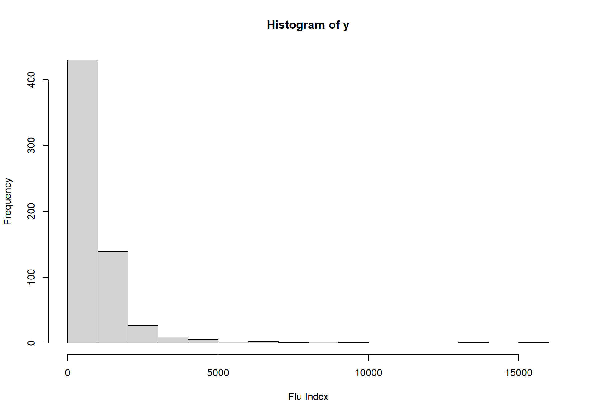
plot(time,y,type='l',ylab="Flu Index",lwd=2,log='y')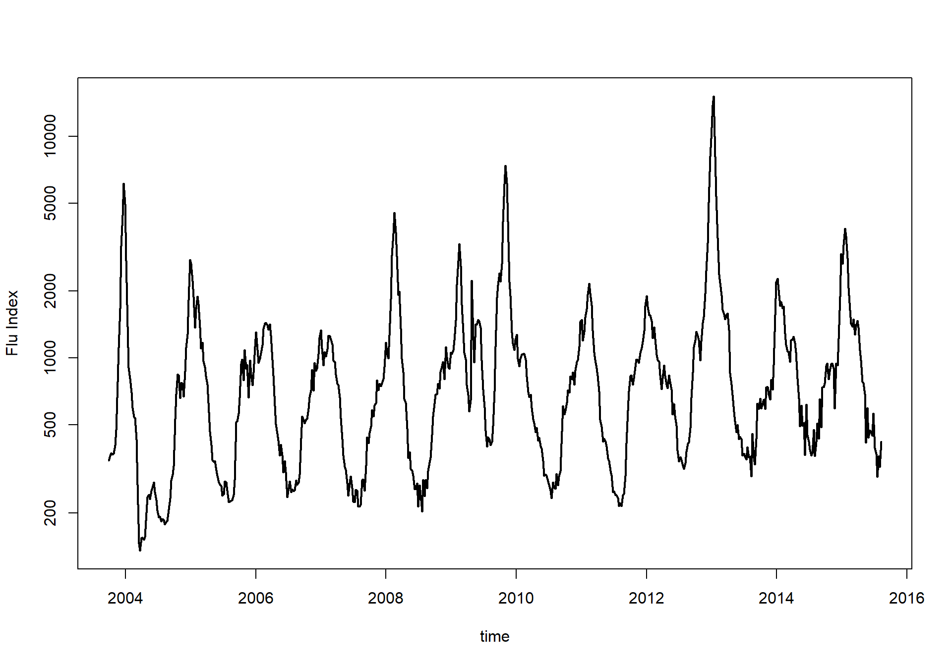
5.3 Random walk & JAGS model
Next we’ll want to define the JAGS code, which we’ll do by writing the code as a string in R. The code itself has three components, the data model, the process model, and the priors. The data model relates the observed data, y, at any time point to the latent variable, x. For this example we’ll assume that the observation model just consists of Gaussian observation error.
\[Y_{t} \sim N(X_{t},\tau_{obs})\]
The process model relates the state of the system at one point in time to the state one time step ahead. In this case we’ll start with the simplest possible process model, a random walk, which just consists of Gaussian process error centered around the current value of the system.
\[X_{t+1} \sim N(X_{t},\tau_{add})\]
Finally, for the priors we need to define priors for the initial condition, the process error, and the observation error.
RandomWalk = "
model{
  #### Data Model
  for(t in 1:n){
    y[t] ~ dnorm(x[t],tau_obs)
  }

  #### Process Model
  for(t in 2:n){
    x[t]~dnorm(x[t-1],tau_add)
  }

  #### Priors
  x[1] ~ dnorm(x_ic,tau_ic)
  tau_obs ~ dgamma(a_obs,r_obs)
  tau_add ~ dgamma(a_add,r_add)
}
"
5.4 Define data and priors
Next we need to define the data and priors as a list. For this analysis we’ll work with the log of the Google flu index since the zero-bound on the index and the magnitudes of the changes appear much closer to a log-normal distribution than to a normal.
data <- list(y=log(y),n=length(y),      ## data
             x_ic=log(1000),tau_ic=100, ## initial condition prior
             a_obs=1,r_obs=1,           ## obs error prior
             a_add=1,r_add=1            ## process error prior
             )
5.5 Define initial conditions
Next we need to definite the initial state of the model’s parameters for each chain in the MCMC. The overall initialization is stored as a list the same length as the number of chains, where each chain is passed a list of the initial values for each parameter. Unlike the definition of the priors, which had to be done independent of the data, the initialization of the MCMC is allowed (and even encouraged) to use the data. However, each chain should be started from different initial conditions. We handle this below by basing the initial conditions for each chain off of a different random sample of the original data.
nchain = 3
init <- list()
for(i in 1:nchain){
  y.samp = sample(y,length(y),replace=TRUE)
  init[[i]] <- list(tau_add=1/var(diff(log(y.samp))),  ## initial guess on process precision
                    tau_obs=5/var(log(y.samp)))        ## initial guess on obs precision
}
5.6 Implement JAGS Model
Now that we’ve defined the model, the data, and the initialization, we need to send all this info to JAGS, which will return the JAGS model object.
j.model   <- rjags::jags.model(file = textConnection(RandomWalk),
                             data = data,
                             inits = init,
                             n.chains = nchain)
## Compiling model graph
## Resolving undeclared variables
## Allocating nodes
## Graph information:
## Observed stochastic nodes: 620
## Unobserved stochastic nodes: 622
## Total graph size: 1249
##
## Initializing modelNext, given the defined JAGS model, we’ll want to take a few samples from the MCMC chain and assess when the model has converged. To take samples from the MCMC object we’ll need to tell JAGS what variables to track and how many samples to take.
## burn-in
jags.out   <- rjags::coda.samples(model = j.model,
                            variable.names = c("tau_add","tau_obs"),
                                n.iter = 1000)
MCMCvis::MCMCtrace(jags.out, pdf = FALSE )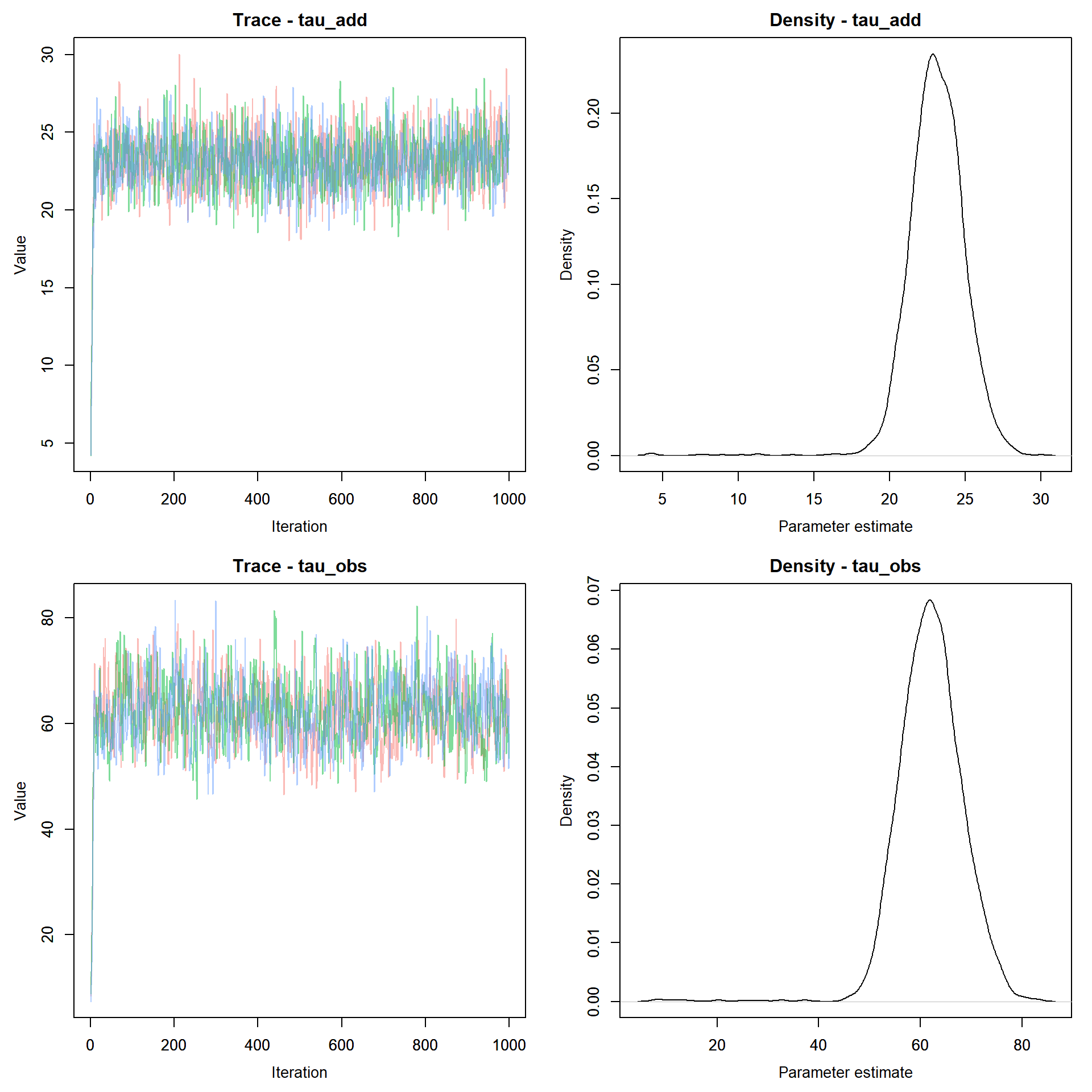
Here we see that the model converges rapidly. Since rjags returns the samples as a CODA object, we can use any of the diagnostics in the R coda library to test for convergence, summarize the output, or visualize the chains.
Now that the model has converged we’ll want to take a much larger sample from the MCMC and include the full vector of X’s in the output
jags.out   <- rjags::coda.samples(model = j.model,
                            variable.names = c("x","tau_add","tau_obs"),
                                n.iter = 10000)
MCMCvis::MCMCtrace(jags.out, params = c("tau_add","tau_obs"), pdf = FALSE )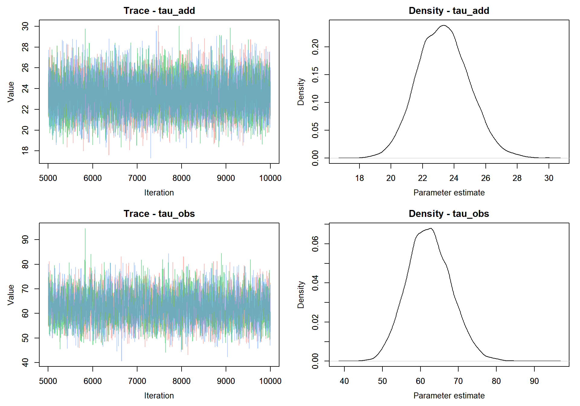
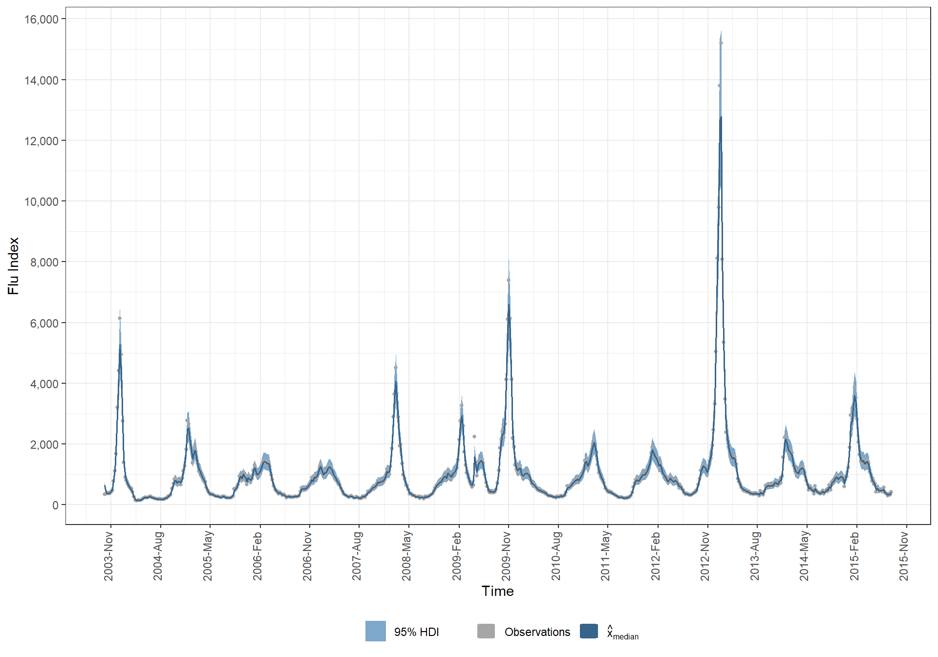
5.7 Visualize output
Given the full joint posterior samples, we’re next going to visualize the output by just looking at the 95% credible interval of the time-series of X’s and compare that to the observed Y’s. To do so we’ll convert the coda output into a matrix and then calculate the quantiles. Looking at colnames(out) will show you that the first two columns are tau_add and tau_obs, so we calculate the CI starting from the 3rd column. We also transform the samples back from the log domain to the linear domain.
5.7.1 Dietze model output
time.rng = c(1,length(time))       ## adjust to zoom in and out
out <- as.matrix(jags.out)         ## convert from coda to matrix
x.cols <- grep("^x",colnames(out)) ## grab all columns that start with the letter x
ci <- apply(exp(out[,x.cols]),2,quantile,c(0.025,0.5,0.975)) ## model was fit on log scale

# plot(time,ci[2,],type='n',ylim=range(y,na.rm=TRUE),ylab="Flu Index",log='y',xlim=time[time.rng])
# ## adjust x-axis label to be monthly if zoomed
# if(diff(time.rng) < 100){
#   axis.Date(1, at=seq(time[time.rng[1]],time[time.rng[2]],by='month'), format = "%Y-%m")
# }
# ecoforecastR::ciEnvelope(time,ci[1,],ci[3,],col=ecoforecastR::col.alpha("lightBlue",0.75))
# points(time,y,pch="+",cex=0.5)
5.7.2 My median model prediction
# data
dplyr::bind_cols(
    time = time
    , y_data = y
    # median x
    , median_x_hat = MCMCvis::MCMCpstr(jags.out, params = "x", func = median) %>% unlist()
    , MCMCvis::MCMCpstr(jags.out, params = "x", func = function(x) HDInterval::hdi(x, credMass = 0.95)) %>%
          as.data.frame()
  ) %>%
  # transform log() by taking exponential
  mutate_at(c("median_x_hat", "x.lower", "x.upper"), exp) %>%
# plot
ggplot(data = ., mapping = aes(x = time)) +
  geom_ribbon(
    mapping = aes(ymin = x.lower, ymax = x.upper, fill = "3")
    , alpha = 0.7
  ) +
  geom_point(
    mapping = aes(y = y_data, color = "1")
    , shape = 16
    , size = 1
  ) +
  geom_line(
    mapping = aes(y = median_x_hat, color = "2")
    , lwd = 0.7
  ) +
  scale_y_continuous(breaks = scales::extended_breaks(n=10), labels = scales::comma) +
  scale_x_date(date_labels = "%Y-%b", breaks = scales::date_breaks(width = "9 month")) +
  scale_fill_manual(values = c("steelblue"), labels = c("95% HDI")) +
  scale_color_manual(values = c("gray65", "steelblue4")
    , labels = c("Observations", latex2exp::TeX("$\\hat{x}_{median}$"))
  ) +
  labs(
    x = "Time"
    , y = "Flu Index"
  ) +
  theme_bw() +
  theme(
    legend.position = "bottom"
    , legend.direction = "horizontal"
    , legend.title = element_blank()
    , axis.text.x = element_text(angle = 90, hjust = .2, vjust = .1)
  ) +
  guides(
    color = guide_legend(override.aes = list(shape = 15,size = 5))
  )
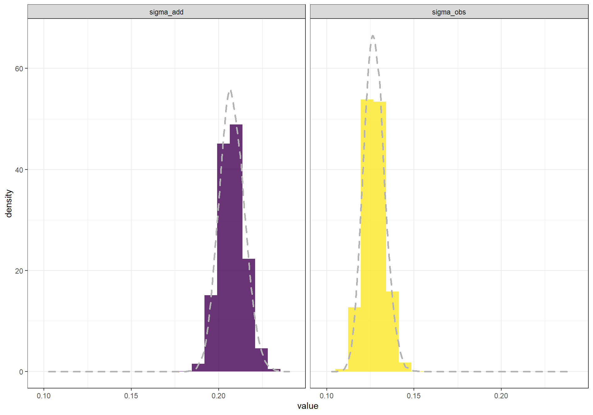
Next, lets look at the posterior distributions for tau_add and tau_obs, which we’ll convert from precisions back into standard deviations.
# Dietze
hist(1/sqrt(out[,1]),main=colnames(out)[1])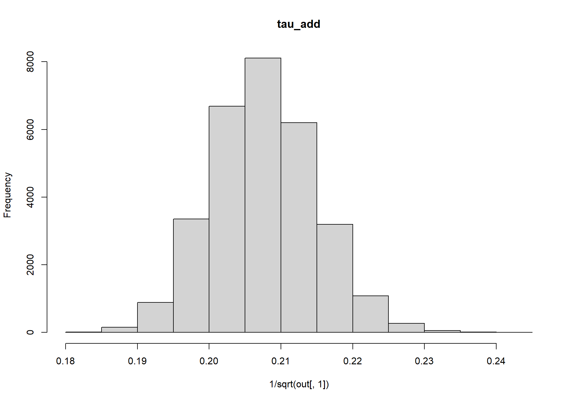
hist(1/sqrt(out[,2]),main=colnames(out)[2])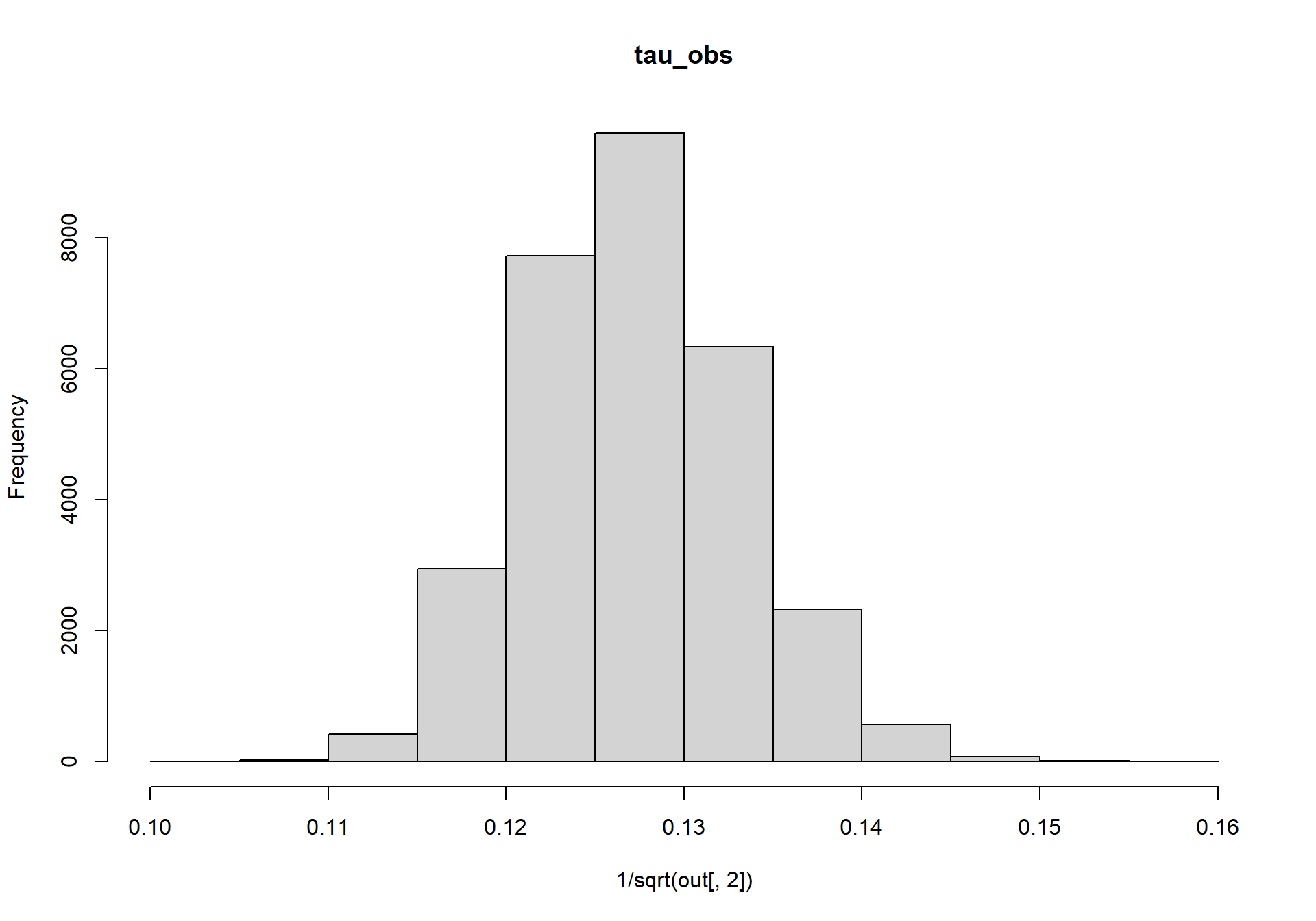
# my updated
sigma_chains_temp <- MCMCvis::MCMCchains(jags.out, params = c("tau_add", "tau_obs")) %>%
  as.data.frame() %>%
  dplyr::mutate(
    sigma_obs = 1/sqrt(tau_obs)
    , sigma_add = 1/sqrt(tau_add)
  ) %>%
  dplyr::select(dplyr::starts_with("sigma")) %>%
  tidyr::pivot_longer(cols = dplyr::starts_with("sigma")) %>%
  dplyr::group_by(name) %>%
  dplyr::mutate(row = row_number()) %>%
  dplyr::ungroup()
# plot
ggplot(sigma_chains_temp, mapping = aes(y = ..density.., x = value)) +
  geom_histogram(
    aes(fill = name)
    , bins = 20
  ) +
  geom_density(
    linetype = 2
    , lwd = 1
    , color = "gray70"
  ) +
  facet_wrap(.~name) +
  scale_fill_viridis_d(alpha = 0.8) +
  theme_bw() +
  theme(
    legend.position = "none"
  )
We’ll also want to look at the joint distribution of the two parameters to check whether the two parameters strongly covary.
# Dietze
plot(out[,1],out[,2],pch=".",xlab=colnames(out)[1],ylab=colnames(out)[2])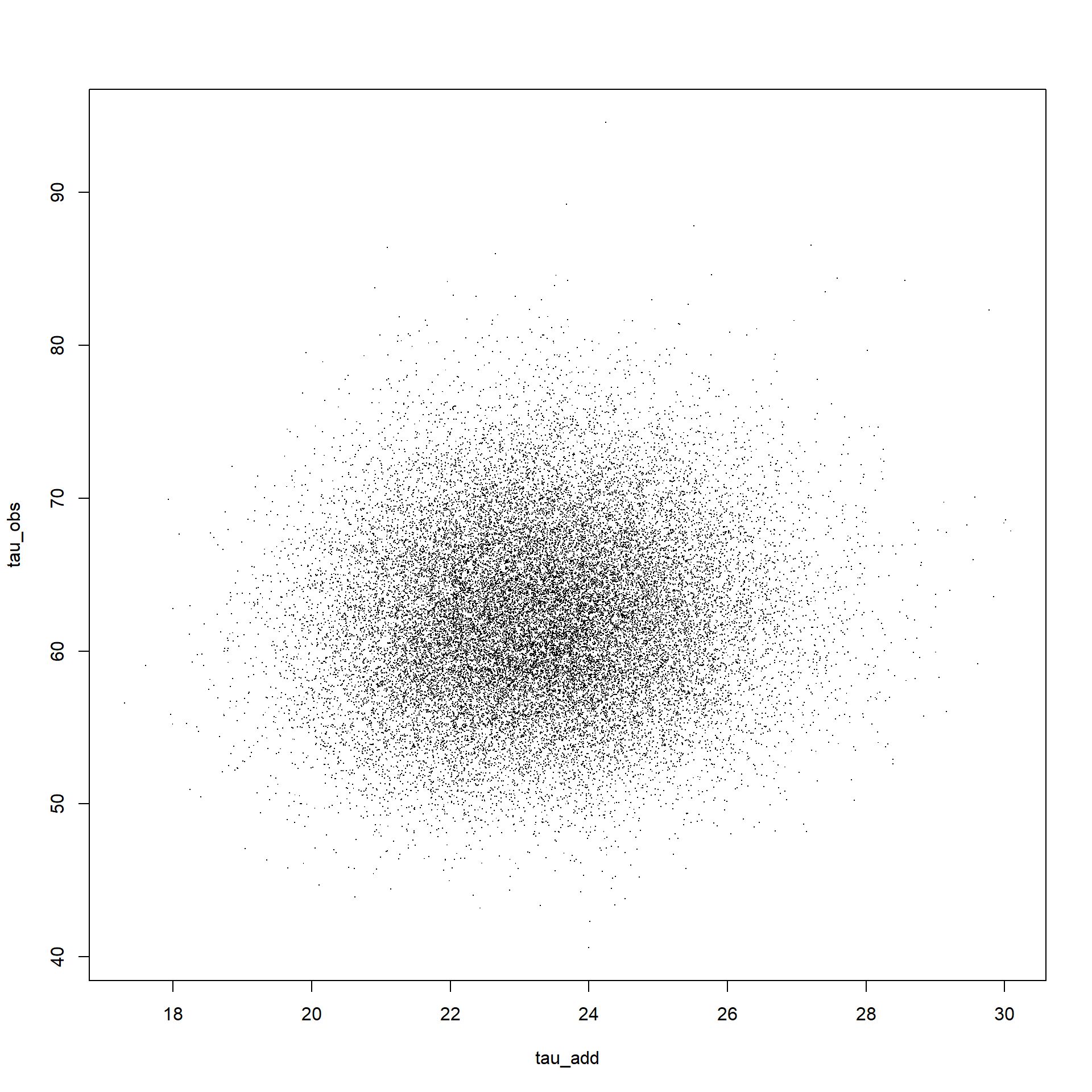
cor(out[,1:2])## tau_add tau_obs
## tau_add 1.00000000 0.08463783
## tau_obs 0.08463783 1.00000000# my updates
sigma_chains_temp %>%
tidyr::pivot_wider(values_from = value, names_from = name) %>%
# plot
ggplot(.) +
geom_point(mapping = aes(y = sigma_obs, x = sigma_add), shape = ".") +
theme_bw()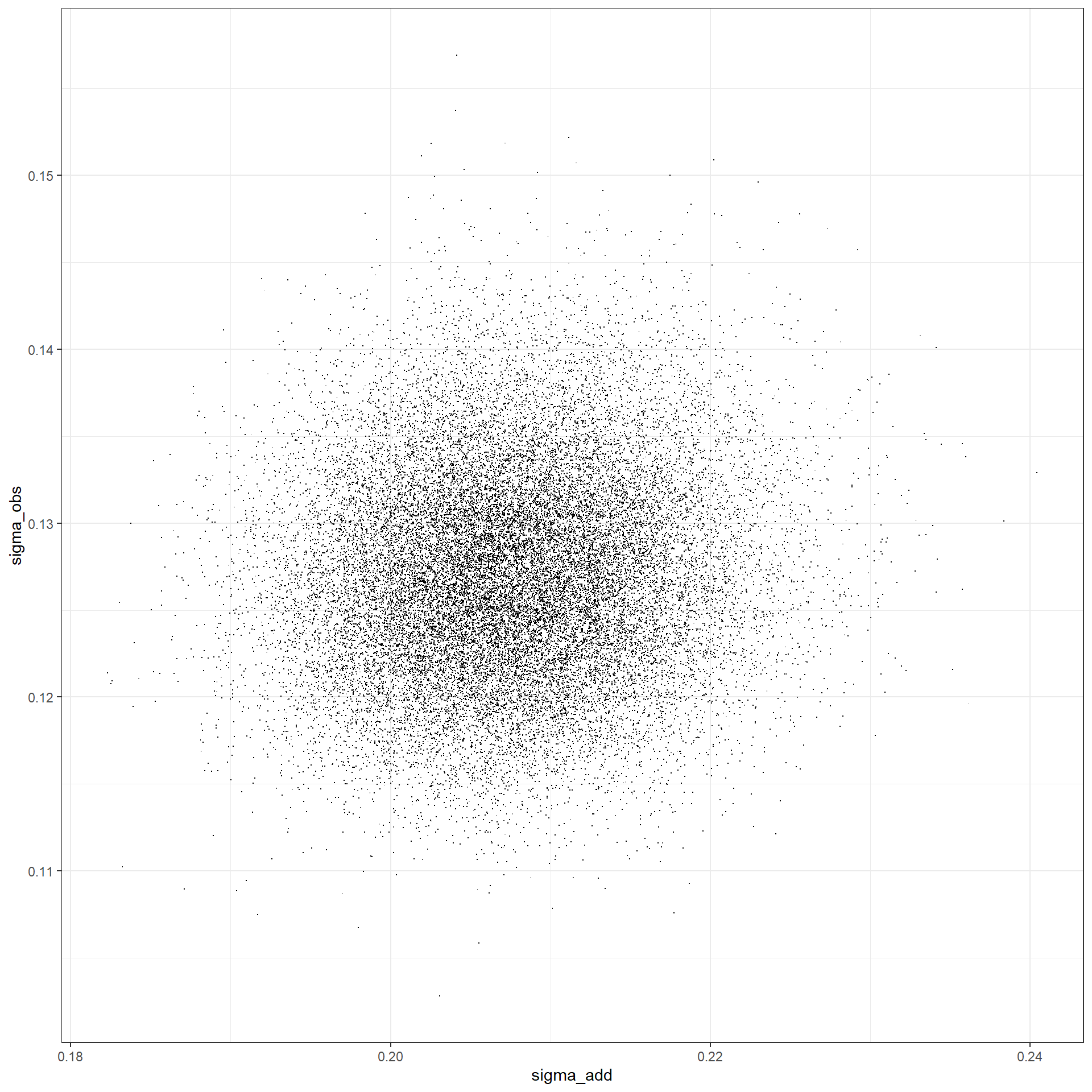
# correlation
sigma_chains_temp %>%
  tidyr::pivot_wider(values_from = value, names_from = name) %>%
  dplyr::select(sigma_obs, sigma_add) %>%
  data.matrix() %>%
  cor()
## sigma_obs sigma_add
## sigma_obs 1.00000000 0.08700835
## sigma_add 0.08700835 1.000000005.8 Questions
To explore the ability of state space models to generate forecasts (or in this case, a hindcast) make a copy of the data and remove the last 40 observations (convert to NA) and refit the model.
# data
y_miss <- c(y[1:(length(y)-40)], rep(as.numeric(NA), 40))
data <- list(y=log(y_miss),n=length(y_miss),      ## data
             x_ic=log(1000),tau_ic=100, ## initial condition prior
             a_obs=1,r_obs=1,           ## obs error prior
             a_add=1,r_add=1            ## process error prior
             )
# inits
nchain = 3
init <- list()
for(i in 1:nchain){
  y.samp = sample(y,length(y),replace=TRUE)
  init[[i]] <- list(tau_add=1/var(diff(log(y.samp))),  ## initial guess on process precision
                    tau_obs=5/var(log(y.samp)))        ## initial guess on obs precision
}
5.8.1 Implement JAGS Model
Now that we’ve defined the model, the data, and the initialization, we need to send all this info to JAGS, which will return the JAGS model object.
j.model_miss   <- rjags::jags.model(file = textConnection(RandomWalk),
                             data = data,
                             inits = init,
                             n.chains = nchain)
## Compiling model graph
## Resolving undeclared variables
## Allocating nodes
## Graph information:
## Observed stochastic nodes: 580
## Unobserved stochastic nodes: 662
## Total graph size: 1249
##
## Initializing modelNext, given the defined JAGS model, we’ll want to take a few samples from the MCMC chain and assess when the model has converged. To take samples from the MCMC object we’ll need to tell JAGS what variables to track and how many samples to take.
jags.out_miss   <- rjags::coda.samples(model = j.model_miss,
                            variable.names = c("x","tau_add","tau_obs"),
                                n.iter = 10000)
MCMCvis::MCMCtrace(jags.out, params = c("tau_add","tau_obs"), pdf = FALSE )
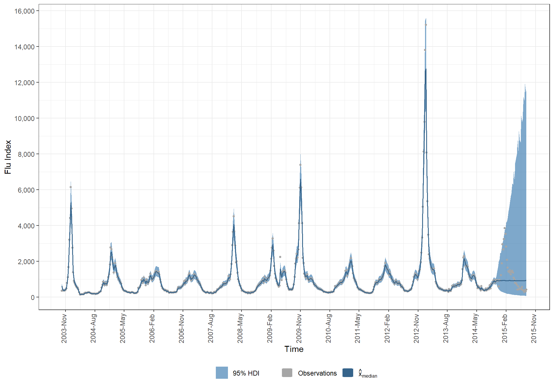
- Generate a time-series plot for the CI of x that includes all the original observed data (as above but zoom the plot on the last ~80 observations). Use a different color and symbol to differentiate observations that were included in the model versus those that were converted to NA’s.
5.8.2 Visualize output
# data
dplyr::bind_cols(
    time = time
    , y_data = y
    # median x
    , median_x_hat = MCMCvis::MCMCpstr(jags.out_miss, params = "x", func = median) %>% unlist()
    , MCMCvis::MCMCpstr(jags.out_miss, params = "x", func = function(x) HDInterval::hdi(x, credMass = 0.95)) %>%
          as.data.frame()
  ) %>%
  # transform log() by taking exponential
  mutate_at(c("median_x_hat", "x.lower", "x.upper"), exp) %>%
# plot
ggplot(data = ., mapping = aes(x = time)) +
  geom_ribbon(
    mapping = aes(ymin = x.lower, ymax = x.upper, fill = "3")
    , alpha = 0.7
  ) +
  geom_point(
    mapping = aes(y = y_data, color = "1")
    , shape = 16
    , size = 1
  ) +
  geom_line(
    mapping = aes(y = median_x_hat, color = "2")
    , lwd = 0.7
  ) +
  scale_y_continuous(breaks = scales::extended_breaks(n=10), labels = scales::comma) +
  scale_x_date(date_labels = "%Y-%b", breaks = scales::date_breaks(width = "9 month")) +
  scale_fill_manual(values = c("steelblue"), labels = c("95% HDI")) +
  scale_color_manual(values = c("gray65", "steelblue4")
    , labels = c("Observations", latex2exp::TeX("$\\hat{x}_{median}$"))
  ) +
  labs(
    x = "Time"
    , y = "Flu Index"
  ) +
  theme_bw() +
  theme(
    legend.position = "bottom"
    , legend.direction = "horizontal"
    , legend.title = element_blank()
    , axis.text.x = element_text(angle = 90, hjust = .2, vjust = .1)
  ) +
  guides(
    color = guide_legend(override.aes = list(shape = 15,size = 5))
  )